Nonparametric estimation of the heterogeneity of a random medium using Compound Poisson Process modeling of wave multiple scattering.

Abstract

In this paper, we present a nonparametric method to estimate the heterogeneity of a random medium from the angular distribution of intensity transmitted through a slab of random material. Our approach is based on the modeling of forward multiple scattering using Compound Poisson Processes on compact Lie groups. The estimation technique is validated through numerical simulations based on radiative transfer theory.

1 Introduction

Small-angle scattering of electromagnetic, acoustic or elastic waves constitutes the basic tool to characterize porous media [1], solid suspensions [2], or Earth’s lithosphere [3], to cite a few examples only. In many cases, the probing wave is assumed to undergo single scattering only and multiple scattering is often considered as a nuisance. The main reason is that in the single-scattering regime, the diffraction pattern of intensity, i.e. the phase function is related to the power spectrum of the medium heterogeneities in a simple manner [4]. In the field of optics, some solutions have been proposed to invert for the size of particles in the multiple-scattering regime [5], based on various small-angle approximations of the radiative transfer equation [6]. In this work, we develop an alternative approach based on the Compound Poisson Process (CPP) model of wave multiple scattering in random media. Our model is generic and makes little assumption on the underlying wave equation. The random medium is described by its heterogeneity power spectrum which refers to the Fourier transform of the spatial two-point correlation function. This enables us to treat on the same footing turbid media like Earth’s crust or the atmosphere, aggregates of particules, and porous media [7]. The finer details of the microstructure encapsulated in higher moments of the random field $(>2)$ are not considered in our approach.

The organization of the paper is as follows: In section II, the necessary mathematical background on non-commutative harmonic analysis is provided. In section III, we develop the Poisson process approach to multiple scattering. In section IV, we validate the model through comparisons with Monte Carlo simulations of the radiative transfer equation. The inverse problem is examined in section V, where we propose an estimator of the power spectrum of heterogeneities and discuss its statistical properties. In section VI, the inverse method is validated for realistic examples of random media through numerical simulations. We consider waves propagating in a turbid medium described by the Von Karman correlation function, which is commonly used to represent geophysical media. We demonstrate the possibility to estimate the power spectrum of the random fluctuations from the angular distribution of intensity transmitted through a slab of material. We find that the CPP model is effective before the diffusive regime sets in, i.e. when the slab thickness is less than one transport mean free path.

2 Noncommutative Harmonic Analysis

In this section, we summarize noncommutative harmonic analysis results that are important for the present work. We are interested in the harmonic analysis of probability density functions (pdf) over compact Lie groups, in order to develop a nonparametric approach for the estimation of their characteristic functions [8], i.e. their Fourier transform, in Section 5.

Consider the direction of propagation of a particule or a wave represented by the normalized vector $\mu\in{\mathcal{S}}^{2}$, where ${\cal S}^{2}$ is the unit sphere in ${\mathbb{R}}^{3}$. We denote by $\mu_{N}$ the direction of propagation of the particule after $N$ scattering events. Such scattering events are considered random so that $\mu_{N}$ is a random variable on ${\cal S}^{2}$. The relation between the direction after $N-1$ scattering events, i.e. $\mu_{N-1}$, and the direction after $N$ scattering events $\mu_{N}$ can be written as:

$$\mu_{N}={\bf r}_{N}\mu_{N-1},$$ (1)

where ${\bf r}_{N}$ is a random element of the rotation group $SO(3)$. This follows from the transitive action of $SO(3)$ on ${\cal S}^{2}$. Assuming that a particule enters the random medium with initial direction of propagation $\mu_{0}$, its direction of propagation after $N$ scattering events in the medium is given by:

$$\mu_{N}={\bf r}_{N}{\bf r}_{N-1}\ldots{\bf r}_{2}{\bf r}_{1}\mu_{0}=\prod_{n=1}^{N}{\bf r}_{n}\mu_{0},$$ (2)

where each ${\bf r}_{n}$ represents the random action of the $n^{th}$ scatterer, i.e. the ${\bf r}_{n}$ are $SO(3)$-valued random variables. In the sequel, we present some results about the pdf of random variables of the form (2). We make use of known results in harmonic analysis on compact Lie groups [9, 10, 11].

2.1 Harmonic analysis on $SO(3)$ and ${\mathcal{S}}^{2}$

Let us denote by ${\cal L}^{2}(SO(3),d{\bf r})$ the space of square integrable functions on $SO(3)$ with respect to the Haar measure $d{\bf r}$ [9]. A probability density function (pdf) on $SO(3)$ is a function $f\in{\cal L}^{2}(SO(3),d{\bf r})$ which obeys the constraint $\int_{SO(3)}f({\bf r})d{\bf r}=1$. A pdf on $SO(3)$ can be decomposed over the complete orthonormal basis of Wigner-D functions $D_{l}^{pq}({\bf r})$, with ${\bf r}\in SO(3)$, $l\in{\mathbb{Z}}^{+}$, $p,q\in{\mathbb{Z}}$. This means that given a random variable ${\bf r}\in SO(3)$, its pdf $f(\bf r)$, can be expressed as the infinite series:

$$f({\bf r})=\sum_{l\geq 0}\sum_{p,q=-l}^{l}(2l+1)\hat{f}_{l}^{pq}\overline{D_{l}^{pq}({\bf r})},$$ (3)

where:

$$\hat{f}_{l}^{pq}=\int_{SO(3)}f({\bf r})D_{l}^{pq}({\bf r})d{\bf r},$$ (4)

and the overbar means complex conjugation. The set of coefficients $\hat{f}_{l}^{pq}$ are sometimes called the “Fourier transform” of $f(\bf r)$ [12]. Note that it is possible to use a matrix notation, namely $\hat{{\bf f}}_{l}$, in which case, the elements of the $(2l+1)\times(2l+1)$ matrix $\hat{\bf f}_{l}$ are: $\left\{\hat{{\bf f}}_{l}\right\}_{pq}=\hat{f}_{l}^{pq}$.

Similarly, let us denote by ${\cal L}^{2}({\cal S}^{2},d\mu)$ the space of square integrable functions on the unit sphere ${\cal S}^{2}$ with respect to the invariant measure on the sphere $d\mu$. A pdf $w\in{\cal L}^{2}({\cal S}^{2},d\mu)$ also satisfies: $\int_{{\cal S}^{2}}w(\mu)d\mu=1$. Similar to Equation (3), a pdf $w$ on ${\cal S}^{2}$ can be decomposed into an infinite series, using the well-known spherical harmonics $Y_{l}^{p}(\mu)$ with $\mu\in{\cal S}^{2}$, $l\in{\mathbb{Z}}^{+}$, $p\in{\mathbb{Z}}$. Thus, given a random variable $\mu\in{\mathcal{S}}^{2}$, its pdf $w(\mu)$ can be written as:

$$w(\mu)=\sum_{l\geq 0}\sum_{p=-l}^{l}(2l+1)\hat{w}^{p}_{l}\overline{Y_{l}^{p}(\mu)},$$ (5)

with:

$$\hat{w}_{l}^{p}=\int_{{\mathcal{S}}^{2}}w(\mu)Y_{l}^{p}(\mu)d\mu.$$ (6)

In this case, it is also possible to use a vector representation, where the elements of the $(2l+1)$ vectors $\hat{{\bf w}}_{l}$ are $\hat{w}_{l}^{p}$ ($p=-l,\ldots,0,\ldots,l$). Again, $\hat{w}_{l}^{p}$ is called the Fourier transform of $w(\mu)$.

We now make use of the following fundamental property: the action of $SO(3)$ on ${\mathcal{S}}^{2}$ is transitive [10]. As a consequence, for any ${\bf r}\in SO(3)$ and $\mu\in{\mathcal{S}}^{2}$, we have ${\bf r}\mu\in{\mathcal{S}}^{2}$. This Lie group action of the rotation group on the unit sphere implies that, given two pdfs $f({\bf r})$ and $w(\mu)$ taking respectively values on $SO(3)$ and ${\mathcal{S}}^{2}$, their convolution is a pdf over ${\mathcal{S}}^{2}$ and reads:

$$h(\mu)=\left(f*w\right)(\mu)=\int_{SO(3)}f({\bf r})w({\bf r}^{-1}\mu)d{\bf r},$$ (7)

for any $\mu\in{\mathcal{S}}^{2}$. A very important and interesting consequence of the Peter-Weyl theorem [9] is that this convolution equation is transformed into a multiplication in the “frequency domain” as follows:

$$h(\mu)=\displaystyle{\sum_{l\geq 0}\sum_{p=-l}^{l}}(2l+1)\hat{h}_{l}^{p}\overline{Y_{l}^{p}(\mu)}.$$ (8)

Using the matrix/vector notation introduced previously, we obtain the following relation:

$$\hat{{\bf h}}_{l}=\hat{{\bf f}}_{l}\hat{{\bf w}}_{l}~{}~{}\forall l,$$ (9)

which is a matrix-vector multiplication taking place for each degree $l$. As explained in [11], two succesive rotations consist in an other rotation ${\bf r}={\bf r}_{2}{\bf r}_{1}$. Moreover the pdf of ${\bf r}$ is the convolution of the pdfs of ${\bf r}_{1}$ and ${\bf r}_{2}$, namely $f_{1}({\bf r}_{1})$ and $f_{2}({\bf r}_{2})$, where convolution is again defined with respect to the group action:

$$f({\bf r})=\int_{SO(3)}f_{2}({\bf t})f_{1}({\bf t}^{-1}{\bf r})d{\bf t}.$$ (10)

In equation (10), ${\bf t}$ denotes an element of $SO(3)$, and $d{\bf t}$ stands for the Haar measure. Consequently, an $N-times$ product of independent random elements of $SO(3)$, i.e. $N$ consecutive random rotations, consists in a random rotation whose pdf is the $N-times$ convolution of the pdfs of the elementary rotations. Thus, if we denote by ${\bf r}={\bf r}_{N}{\bf r}_{N-1}\ldots{\bf r}_{2}{\bf r}_{1}$ the outcome of $N$ successive rotations, the Fourier transform of ${\bf r}$ can be expressed as follows:

$$\hat{{\bf f}}_{l}=\displaystyle{\prod_{n=1}^{N}\left(\hat{{\bf f}}_{n}\right)_{l}}~{}~{}\forall l.$$ (11)

which is a simple product of matrices. In (11), $\left(\hat{{\bf f}}_{n}\right)_{l}$ denotes the matrix of Fourier coefficients of degree $l$ of $f_{n}$, the pdf of ${\bf r}_{n}$.

2.2 Symmetries

Using Eq. (9) and (11), it is possible to obtain the Fourier coefficients of any distribution on ${\cal S}^{2}$ that was multiply convolved by pdfs on $SO(3)$. In what follows, we will derive more specific results for distributions on ${\cal S}^{2}$ which are functions of $\mu=\cos\theta$ only, with $\theta$ the scattering angle. Such functions are called zonal functions on ${\cal S}^{2}$ [9]. This simplification relies on the property of statistical isotropy of the random medium. As a consequence, the Fourier transform over ${\cal S}^{2}$ reduces to a Legendre expansion over $[-1;1]$ for zonal functions. In anisometric random media where the correlation length depends on space direction, this simplification is not permitted.

In order to obtain simple results, we further impose that the initial distribution of directions of propagation $\mu_{0}$ is a zonal function. Such an assumption is not too restrictive and covers for example the case of an incident plane wave, i.e. $\mu_{0}$ is a Dirac distribution. Using the ${\cal XZX}$ parametrization of $SO(3)$ [12], the symmetry of the scattering process around the direction of propagation implies that the pdf $w_{\mu}(\mu)$ of the direction of propagation $\mu$, parametrized using co-elevation $\theta$ (with respect to direction of propagation) and azimuth $\varphi$, is invariant with respect to $\varphi$. This allows us to expand $w_{\mu}(\mu)$ as follows:

$$w_{\mu}(\mu)=\displaystyle{\sum_{l\geq 0}(2l+1)\hat{w}_{l}^{0}\overline{Y_{l}^{0}(\mu)}=\sum_{l\geq 0}(2l+1)\hat{w}_{l}P_{l}(\cos\theta)},$$ (12)

where the $\hat{w}_{l}$ are scalar quantities. The rotational symmetry of the scattering process also implies that the pdf $f({\bf r})$ of random elements of $SO(3)$ must be bi-invariant, i.e. invariant by left and right action on $SO(3)$ (see [9] for details). Such a bi-invariant pdf $f({\bf r})$ depends on a single variable $\mu=\cos\theta$, and can therefore be expanded as:

$$f({\bf r})=\displaystyle{\sum_{l\geq 0}}(2l+1)\hat{f}_{l}^{00}\overline{D_{l}^{00}({\bf r})}=\sum_{l\geq 0}(2l+1)\hat{f}_{l}P_{l}(\cos\theta).$$ (13)

Considering the successive action of $N$ i.i.d. random rotations on the initial distribution of propagation directions $\mu_{0}$ leads to the following expression of the pdf $h(\mu_{N})$ of $\mu_{N}={\bf r}_{N}{\bf r}_{N-1}\ldots{\bf r}_{2}{\bf r}_{1}\mu_{0}$:

$$h(\mu_{N})=\displaystyle{\sum_{l\geq 0}}(2l+1)(\hat{f}_{l})^{N}\hat{w}_{l}P_{l}(\mu).$$ (14)

In the special case of an incident plane wave or a highly collimated beam, the initial direction obeys the following simple probability distribution $w(\mu_{0})=\delta(\mu-\mu_{z})$ where $\mu_{z}$ is the vector pointing in the direction of propagation. Introducing this expression of $w$ in Equation (12) yields: $\hat{w}_{l}=P_{l}(\mu_{z}).$ By symmetry $\mu_{z}$ must coincide with the co-latitude 0, i.e. the north pole $\theta=0$, which implies $\hat{w}_{l}=1$, $\forall l$. In such a case, eq. (14) becomes:

$$f(\mu_{N})=\displaystyle{\sum_{l\geq 0}}(2l+1)(\hat{f}_{l})^{N}P_{l}(\mu)$$ (15)

The pdf of $\mu_{N}$ possesses a simple Legendre expansion with coefficients equal to the $N$th power of the Legendre coefficients $\hat{f}_{l}$ of the $SO(3)$ random variables.

Note that Equation 15 could have been obtained using the well-known summation formula for Jacobi polynomials (see Chapter 2 in [9]) in the case of zonal functions on the sphere. The approach developed in this section is more general because it could be applied to less symmetrical distributions, thereby allowing the modeling of more complicated scattering processes.

3 The Compound Poisson Process model for multiple scattering

In this section, we develop the multiple scattering model. We begin with a summary of useful results about Compound Poisson Processes (CPP) on compact Lie groups [13]. Note that we use the term $pdf$ when we refer to the function describing the angular pattern of scattering. In Section 4, we will substitute it with phase function which is the usual terminology in the field of scattering in random media.

3.1 The model

The implementation of the CPP model for the study of multiple scattering of particules/waves has already been described in [14]. In [14], the authors were mostly interested in formulating the direct problem, i.e. in the way a CPP can be used to predict the output distribution of scattering angles in a scattering experiment. They demonstrated the ability of the CPP to model the multiple scattering of electrons and used some recursive integral equations to obtain the pdf of the CPP. The CPP model introduced in [14] is based on the cumulative scattering angle, which is a real valued random process defined as a sum of real-valued random variables. In this work, we introduce a CPP on a compact Lie group, namely the rotation group $SO(3)$. Our approach is more general and does not rely on an a priori small-angle approximation.

Let us consider a particule/wave entering a random medium at time $t=0$, with initial direction of propagation $\mu_{0}\in{\cal S}^{2}$, as illustrated in Figure 1. For the moment we neglect the possibility that the wave may escape the random medium. We consider a slab of random material with mean free time $\tau$ and velocity $c=1$ for simplicity. The normalization of the velocity implies $\lambda=1/\ell$ where $\ell$ is the mean free path. We seek to model the time evolution of the direction of propagation $\mu(t)$. Denoting by $N(t)$ the random number of scattering events that have occurred after propagation during time $t$ in the random medium, the direction of propagation $\mu(t)$ can be written as:

$$\mu(t)=\prod_{n=0}^{N(t)}{\bf r}_{n}\mu_{0}.$$ (16)

In order to model wave scattering, $N(t)$ is chosen as a Poisson process, and is independent of the ${\bf r}_{n}$. To be fully consistent, we must impose ${\bf r}_{0}=\mathbf{I}$, where $\mathbf{I}$ denotes the identity in $SO(3)$. This simply means that the unscattered energy propagates in the direction imposed by the source. Clearly, the ${\bf r}_{n}$, $n\geq 1$ are independent and identically distributed random rotations described by the pdf $f({\bf r})$. Our choice for $N(t)$ implies the usual exponential distribution of times of flight between two scattering events, with parameter $\lambda=1/\tau$.

3.2 Probability density function of the CPP

To complete our task, we need to relate the pdf of $\mu(t)$, denoted by $p(\mu(t))$, to the scattering properties of the medium. Keeping in mind the i.i.d. assumption for ${\bf r}_{n}$ and using conditional probability decomposition with respect to the Poisson process $N(t)$, one gets:

$$p(\mu(t))=\sum_{n=0}^{\infty}e^{-\lambda t}\frac{(\lambda t)^{n}}{n!}f^{\otimes n}({\bf r})*w(\mu_{0}),$$ (17)

where $\otimes n$ denotes the $n-times$ convolution, $f({\bf r})$ is the common distribution of the ${\bf r}_{n}$ and $w(\mu_{0})$ is the distribution of $\mu_{0}$. Making use of the notation introduced in Section 2.1 for the multiple action of ${\bf r}_{i}$: $\mu_{n}={\bf r}_{n}{\bf r}_{n-1}\ldots{\bf r}_{2}{\bf r}_{1}{\bf r}_{0}\mu_{0}$, the pdf of $\mu_{n}$ can be rewritten as:

$$f(\mu_{n})=f^{\otimes n}({\bf r})*w(\mu_{0}).$$ (18)

Assuming again that the distribution of $\mu_{0}$ is a Dirac at the north pole, the distribution of $\mu(t)$ simplifies to:

$$p(\mu(t))=\displaystyle{\sum_{n=0}^{\infty}\frac{(\lambda t)^{n}}{n!}e^{-\lambda t}f^{\otimes n}({\bf r})}.$$ (19)

The assumption about $\mu_{0}$ is not very strong since in many practical cases the direction of propagation of the incoming wave is either known or controlled. For an isotropic random medium, we recall that the pdfs of ${\bf r}_{i}$ can be considered zonal. Therefore, the pdf $f({\bf r})$ can be expanded in a Legendre series with coefficients denoted by $\hat{f}_{k}$. Using eq. (15) the pdf of $\mu(t)$ takes the form:

$$\begin{array}[]{rcl}p(\mu(t))&=&\displaystyle{\sum_{n=0}^{\infty}\frac{(\lambda t)^{n}}{n!}e^{-\lambda t}\sum_{l\geq 0}(2l+1)\left(\hat{f}_{l}\right)^{n}P_{l}(\mu)}\\ &&\\ &=&\displaystyle{e^{-\lambda t}\sum_{l\geq 0}(2l+1)e^{\lambda t\hat{f}_{l}}P_{l}(\mu)}\end{array}.$$ (20)

This provides an expression of the distribution of $\mu(t)$ of the form:

$$p(\mu(t))=\displaystyle{\sum_{l\geq 0}(2l+1)e^{\lambda t(\hat{f}_{l}-1)}P_{l}(\mu)}.$$ (21)

Expanding $p(\mu(t))$ in a Legendre series:

$$p(\mu(t))=\displaystyle{\sum_{l\geq 0}(2l+1)\hat{\mu}_{l}P_{l}(\mu)},$$ (22)

a term-by-term identification in Equations (21) and (22) yields:

$$\hat{\mu}_{l}=e^{\lambda t(\hat{f}_{l}-1)}.$$ (23)

The result (23) relates directly the Legendre coefficients $\hat{\mu}_{l}$ of the pdf of the scattering process $\mu(t)$ to the Legendre coefficients $\hat{f}_{l}$ of the pdf of the random rotations caused by the scatterers. This close link between the Fourier coefficients of these pdfs is the cornerstone of our approach as it enables us to develop a statistical estimator of the Fourier coefficients $\hat{f}_{l}$, from the observations of the pdf of $\mu(t)$.

4 Validity of the CPP model

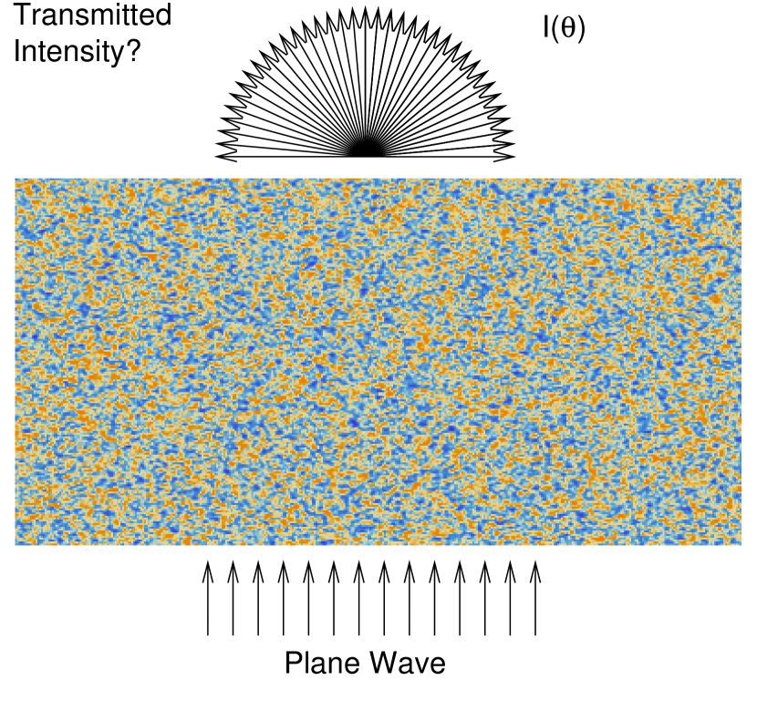
Figure 1: Position of the problem. A plane wave or a narrow beam are normally incident on a slab of random heterogeneous material with thickness $z$ expressed in transport mean free path units. The transmitted intensity probability distribution is $I(\theta)$.

4.1 Models of random media

In order to show the applicability of our statistical approach, we consider the following experiment (see Figure 1): A plane wave or narrow beam is normally incident on a slab of random material described by Von Karman or Gaussian spectra, which are commonly used to describe geophysical media [15]. The angular pattern of intensity transmitted through the slab is measured on output. In the slab geometry with strong forward scattering, we expect that most of the energy will be collected in the forward direction and therefore the CPP should give some useful predictions of the pattern of transmitted intensity. In fact, this idea is confirmed by the agreement between the CPP formula (21) and small-angle scattering approximations of the radiative transfer equation [6]. It is to be noted that formula (21) was obtained under the hypothesis that we are able to collect all the energy at a given time $t$ but is totally free from a small-angle scattering assumption.

In the CPP approach, the building block for multiple scattering is the pdf of the random rotations that scatter the initial direction of the incoming beam. In the language of scattering theory, the function that describes the angular scattering pattern is called the phase function and will be denoted by $f(\mu)$, where $\mu=cos(\theta)$ is the cosine of the scattering angle. For sufficiently weak fluctuations, the phase function can be obtained from the Born approximation [4] and depends of the power spectrum of heterogeneities $\Phi$ as follows:

$$f(\mu)=c\Phi\left(2k\sin({\theta/2})\right),$$ (24)

where $k$ denotes the central wavenumber of the probing wave, and $c$ is a normalization constant. For the sake of clarity, we review basic results on random media of special interest.

4.1.1 Gaussian Media

The phase function of a Gaussian random medium is defined by the following formula:

$$f(\mu)=\frac{k^{2}a^{2}}{2(1-e^{-k^{2}a^{2}})}e^{-k^{2}a^{2}\frac{(1-\mu)}{2}},$$ (25)

where $a$ is the correlation length of heterogeneities. The anisotropy parameter or mean cosine of the scattering angle is defined as:

$$g=\int\limits^{1}_{-1}f(\mu)\mu d\mu.$$ (26)

This parameter plays a crucial role in the definition of the transport mean free path $l^{*}=l/(1-g)$. The transport mean free path is the typical length scale beyond which multiple scattering can be described by a diffusion equation. In the common case of strong forward scattering it can be much larger than the mean free path. As will be shown below, our approach is useful in this regime. For Gaussian random media, one obtains $g=\coth\left(\frac{k^{2}a^{2}}{2}\right)-\frac{2}{k^{2}a^{2}}$. The Legendre coefficients of the phase function are given by:

$$\hat{f}_{l}=\int f(\mu)P_{l}(\mu)d\mu.$$ (27)

In the high-frequency limit (large $ka$), the Legendre coefficients of the Gaussian phase function can be approximated as:

$$\hat{f}_{l}\approx g^{l(l+1)/2},$$ (28)

with $g\approx 1-1/2k^{2}a^{2}$.

4.1.2 Von Karman Media

The Von Karman spectrum implies the following angular dependence of the phase function:

$$f(\mu)=\frac{2k^{2}a^{2}(\alpha-1)}{\left(1-\left(4k^{2}a^{2}+1\right)^{1-\alpha}\right)\left(1-2k^{2}a^{2}(\mu-1)\right)^{\alpha}},$$ (29)

where $\alpha$ is an exponent which controls the small-scale roughness of the medium. Note that the phase function is normalized ($\int\limits_{-1}^{1}f(\mu)d\mu=1$). The special cases $\alpha=3/2,2$ correspond to the well-known Henyey-Greenstein and exponential phase functions, respectively.

Using integration by parts, the coefficients of the expansion can be expressed as:

$$\hat{f}_{l}=\frac{1}{2^{n}n!}\int\limits^{1}_{-1}(1-\mu^{2})^{l}f^{(l)}(\mu)d\mu,$$ (30)

where $f^{(l)}(\mu)$ denotes the $l^{th}$ derivative of the phase function. Using tables of integrals, (30) yields the following compact form for the Legendre coefficients of the Von Karman correlation function:

$$\begin{split}\hat{f}_{l}=&\frac{\displaystyle 2\sqrt{\pi}(\alpha-1)(1+2ka^{2})^{-(l+\alpha)}\Gamma(l+\alpha)}{\displaystyle\Gamma\left(\frac{3}{2}+l\right)\Gamma(\alpha)(1-(1+4ka^{2})^{1-\alpha})}\\ &\times~{}{}_{2}F_{1}\left(\frac{l+\alpha}{2},\frac{1+l+\alpha}{2};\frac{3}{2}+l;\frac{4ka^{4}}{(1+2ka^{2})^{2}}\right)\end{split}.$$ (31)

where the definition of the hypergeometric function $~{}{}_{2}F_{1}$ can be found in [16]. As noted before, in the case $\alpha=3/2$, we recover the Henyey-Greenstein (HG) phase function which is a classically used approximation to the Mie theory for spherical scatterers. The Legendre coefficients can be put in the form $\hat{f}_{l}=g^{l}$, with $g=(1+2k^{2}a^{2}-\sqrt{1+4k^{2}a^{2}})/2k^{2}a^{2}$, i.e. the Legendre coefficients are simply powers of the anisotropy parameter, valid for any $g\in[0,1[$. A remarkable property of HG random media is that the convolution on the sphere of unit directions of $n$ HG phase functions with same parameter $g$, is a itself a HG phase function with parameter $g^{n}$:

$$f_{HG}^{\otimes n}(\mu)=\sum_{l=0}^{\infty}(2l+1)g^{ln}P_{l}(\mu).$$ (32)

4.2 Numerical results

Figure 2: Comparison between Monte Carlo simulations (dots) and CPP model for the intensity transmitted through a slab of random medium with Heynyey-Greenstein phase function. The four curves correspond to increasing slab thicknes $H=25/8,25/4,25/2,25\ell$, with $\ell$ the mean free path. The agreement is very good in a cone around the forward direction and degrades as the scattering angle approaches grazing angles.

In order to appreciate the strengths and weaknesses of our statistical model we show direct comparisons between the CPP and the radiative transfer equation for a Henyey-Greenstein random medium in the strong forward-scattering regime. The anisotropy factor is $g=0.98$ and the slab thickness takes the values $H=25/8,25/4,25/2,25\ell$, where $\ell$ is the mean free path of the waves in the random medium (the transport mean free path $\ell^{*}$ equals $50\ell$). For simplicity, we assume that the index of the slab matches that of the surrounding medium. The equation of radiative transfer is solved using the Monte Carlo code developed by [17] in the framework of statistically anisotropic media. Figure (2) shows that the CPP model gives a non-uniform approximation to the exact distribution of intensity transmitted through the slab of random material. It is noticeable that the CPP model is always wrong in a cone of directions perpendicular to the direction of incidence of the wave. The width of the cone of direction increases with the slab thickness $H$. When $H$ becomes of the order of the transport mean free path, typically, the CPP model fails to give reliable predictions of the angular distribution of intensity. One obvious reason is that in the CPP model, we do not prescribe any boundary condition whereas in the slab geometry, the intensity must of course vanish in the lower hemisphere of propagation directions.

We further remark that in the slab geometry the distribution of scattering events does not follow a simple Poisson law, which also limits the validity of our model. To illustrate this point, we examine the validity of the model in Figure 3, where we show the comparison between the CPP and radiative transfer theory for a Gaussian medium with anisotropy parameter $g=0.98$. The slab thickness takes the values $H=25/16,25/8,25/4,25/2\ell$. The distribution of transmitted intensity differs markedly from the H-G case (see Figure 2 for comparison). Because the Gaussian medium is extremely smooth, the single scattering pattern is concentrated in a small cone of directions and large-angle scattering is excluded. Propagation at large angle can only occur for sufficiently high-order multiple-scattering. This entails a significant deviation of the statistics of the number of scattering events from the simple Poisson distribution. This point is illustrated in Figure 4, where we plot the distribution of scattering events around the forward direction ($0.8<\mu<1$) and at large angles ($0.3<\mu<0.5$) for particles propagating through a slab of thickness $H=25/8\ell$. While in the forward direction the agreement between the calculated distribution of number of scattering events and Poisson statistics is excellent, at large angles a clear discrepancy is observed. The distribution is biased towards larger number of scattering events and we verified empirically that it is in fact much better fitted by a normal distribution. The standard deviation and mean of the Gaussian distribution have been adjusted by trial and error. The main point is to illustrate the large deviation from the Poisson distribution. Note however that the Poisson law will always be well approximated by a normal distribution (with equal mean and variance) if the number of scattering events becomes very large.

Figure 3: Comparison between Monte Carlo simulations (dots) and CPP model for the intensity transmitted through a slab of random medium with gaussian phase function. The four curves correspond to increasing slab thicknes $H=25/16,25/8,25/4,25/2\ell$, with $\ell$ the mean free path. The agreement is very good in a cone around the forward direction and degrades as the scattering angle approaches grazing angles.

Figure 4: Distribution of the number of scattering events for the intensity transmitted through a slab of gaussian random medium with thickness $H=3.125\ell$. Squares: ($0.8<\mu<1$); dots: ($0.3<\mu<0.5$). Solid line: Poisson distribution with parameter $\lambda=3.125$. Dashed line: Gaussian ditribution with mean $\mu=7$ and standard deviation $\sigma=2$.

We now discuss briefly the transition towards the diffusive regime. The case of strongly anisotropic scattering has been treated analytically in [18], where it is shown that the pattern of transmitted intensity is almost universal, independent of the type of scatterers. In Figure 5, we show the profile of transmitted intensity obtained with the radiative tranfer approach with the slab thickness $H=\ell^{*}/2$ for the Gaussian and H-G phase functions with the same anisotropy parameter $g=0.98$. The curves for the two different phase functions are hardly distinguishable. For comparison, we have also plotted the simple outcome of the diffusion approximation $I(\mu)=\mu(1/2+3\mu/2)$. Our numerical study confirms the general conclusions of [18] and also demonstrates that the diffusive regime sets in for a slab thickness of the order of $\ell^{*}$ but not more.

Figure 5: Transmitted intensity profile through a slab of thickness $H=\ell^{*}/2$ and anisotropy parameter $g=0.98$. Squares: Gaussian random medium. Solid line: H-G random medium. Dashed line: diffusion approximation. The difference between the Gaussian and H-G medium is only noticeable close to the forward direction ($\mu=1$).

In spite of all its deficiencies, the CPP model gives a simple, almost analytical solution of the multiple scattering problem and explains accurately the angular distribution of most of the forward-scattered energy.

5 Estimation: the inverse problem

In this section, we consider the problem of estimating the Legendre coefficients of the phase function $f$ of the scatterers from the measurement of the output angular distribution $p(\mu(T))$ at a given depth in the random medium. Using the CPP model, we can construct an estimator for the Legendre coefficients of the phase function $\hat{f}_{l}$, using a “decompounding” formula. Note that the mean free time $\tau$ or equivalently (thanks to velocity normalization) the mean free path $\ell$ has to be known in the decompounding approach. Techniques to estimate the mean free path of waves in transmission geometry are described for instance in [19]. The estimators we derive below are extensions of the work done in [20, 21] for real valued random variables, to the specific case of random variables taking values over the rotation group and having zonal pdfs.

5.1 Estimator for the Legendre coefficients

After proper normalization, the transmitted intensity profile can be interpreted as a pdf $p(\mu(T))$, where $T$ is the time required for ballistic waves to propagate through the slab. Let us denote by $\overline{p}(\mu(T))$ the sample pdf which corresponds to the data. The sampling resolution of $\overline{p}(\mu(T))$ depends on the acquisition system. Typically, a detector has finite aperture and therefore averages the intensity over some finite solid angle $d\Omega$. This implies that $\overline{p}(\mu(T))$ is in fact discrete and should be more appropriately termed probability mass function with the usual normalization $\sum_{m=1}^{M}\overline{p}(\mu_{m}(T))=1$ if $M$ samples are available.

We are interested in estimating the Legendre coefficients of the pdf $p(\mu(T))$, from the observation of $\overline{p}(\mu_{m}(T))$. This can be achived in two different ways. One can either define directly the estimator on $\overline{p}(\mu(T))$, or use $\overline{p}(\mu(T))$ to generate some realizations of $\mu(T)$ and define an estimator with these realizations. In this paper, we adopt the second approach. To do so, we use a simple linear interpolation to evaluate numerically the cumulative distribution function (cdf) and its inverse from the data $\overline{p}(\mu(T))$. This allows us to generate as many realizations of $\mu(T)$ as desired, by evaluating the inverse cumulative distribution function for a collection of uniformly distributed random numbers in $[0,1]$.

Let us assume that we have generated ${\rm K}$ values of $\mu(T)$ using this technique and let us denote them by $\mu_{\kappa}(T)$ with $\kappa=1,\ldots,{\rm K}$. The empirical Legendre coefficients of $p(\mu(T))$, denoted by $\widetilde{\hat{\mu}}_{l}$ are given by:

$$\widetilde{\hat{\mu}_{l}}=\frac{1}{{\rm K}}\sum_{\kappa=1}^{{\rm K}}P_{l}(\mu_{\kappa}(T)).$$ (33)

This estimator is unbiased, i.e. ${\mathbb{E}}[\widetilde{\hat{\mu}_{l}}-\mu_{l}]=0~{},\forall~{}l$. This means that the mean value of our estimator is the real value we are looking for, i.e. $\hat{\mu}_{l}$. The variance of the estimator can be expressed as:

$${\mathbb{E}}\left[\left(\widetilde{\hat{\mu}_{l}}-{\mathbb{E}}[\widetilde{\hat{\mu}_{l}}]\right)^{2}\right]=\frac{1}{{\rm K}}\left({\mathbb{E}}[P^{2}_{l}(\mu)]-\hat{\mu}_{l}^{2}\right).$$ (34)

where ${\mathbb{E}}[P^{2}_{l}(\mu)]=\int_{-1}^{1}p(\mu(T))P^{2}_{l}(\mu)d\mu$.

In the Gaussian case, the variance takes a simple analytical form, in the limit case where $(g-1)\ll 1$. Using a Taylor series expansion of the Legendre polynomials near $\mu=1$ yields $Var(\widetilde{\hat{\mu}_{l}})=\frac{1}{K}\frac{l^{2}(l+1)^{2}}{4}(g-1)^{2}$. For other random media, such as Henyey-Greenstein or exponential, an analytical expression of the variance is not easily obtained. This is also applies to Gaussian media, away from the limiting case mentioned above. Nevertheless, the behaviour of the variance can be obtained by numerical integration. In Figure 6, we present the variance for three different phase functions: Exponential, Gaussian and Henyey-Greenstein. The estimation has been made using $K=1000$ samples. It can be seen on Figure 6 that the variance of the estimator increases monotonically with $l$ for the three different phase functions. While the Gaussian case follows a $4^{th}$ degree polynomial growth, Henyey-Greenstein and Exponential cases follow a more or less linear increase with the degree of the Legendre coefficients $l$. The Gaussian case is favorable for low degree coefficients while Henyey-Greenstein exhibits the lowest variance for higher degrees. Note that the variance has consequences on the ability of the proposed approach to evaluate correctly the high-degree Legendre coefficients. This will be illustrated in Section 5.2.

Figure 6: Variance of the Legendre coefficients empirical estimator for different phase functions: Gaussian (squares), Exponential (triangles) and Henyey-Greenstein (circles) with anisotropy parameter $g=0.995$.

Back to the “decompounding” problem, we wish to estimate the Legendre coefficients of $f$ from the samples $\mu_{\kappa}(T)$. This is possible by inverting eq. (23) and using our empirical estimator (33). We obtain an estimate of the Legendre coefficients of the phase function of the medium:

$$\widetilde{\hat{f}_{l}}=\frac{1}{\lambda T}\ln\widetilde{\hat{\mu}_{l}}+1.$$ (35)

Equation (35) is the “decompounding” formula. It implies that the set of Legendre coefficients $\widetilde{\hat{f}_{l}}$ can be estimated from the set $\widetilde{\hat{\mu}_{l}}$ which is directly computed from the data thanks to eq. (33). Note that it is necessary that $\widetilde{\hat{\mu}_{l}}>0$. This is verified for small $l$ ($\mu_{0}>\mu_{l}$, $\forall l\geq 1$) but may not be verified for higher degrees, mainly because of the increase of the variance of the estimator $\widetilde{\hat{\mu}_{l}}$ with $l$ (see Figure 6). As a consequence, it will be necessary to truncate the number of Legendre coefficients used in the decompounding approach. The truncation degree depends on the acquisition set-up and the kind of medium investigated. This will be further illustrated in the following Section. It must be emphazised that equation (35) is central as it allows direct estimation of the heterogeneity spectrum of the medium from the output intensity distribution measurement.

5.2 Inverting for the random medium power spectrum

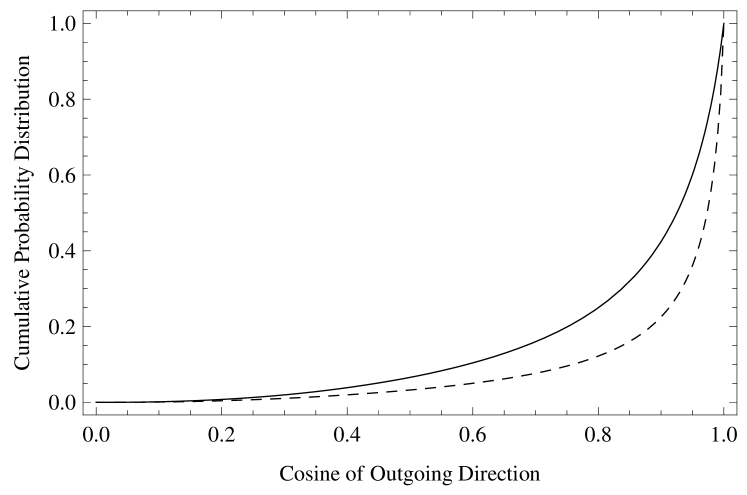
Figure 7: Cumulative distribution function of the intensity transmitted through a slab of random material with thickness $H=6.25\ell$ (dashed line) $12.5\ell$ (solid line) and anisotropy parameter $g=0.98$. Top: exponential medium. Bottom: “Kolmogorov” medium.

Figure 8: Estimated Legendre coefficients of the heterogeneity power spectrum for two slabs of random material with thickness $H=6.25\ell$ (dots), $12.5\ell$ (squares) and anisotropy parameter $g=0.98$. Top: exponential medium. Bottom: “Kolmogorov” medium. The dashed line shows the exact Legendre coefficients of the distributions.

As we will now show, the CPP approach constitutes a powerful tool to invert the power spectrum of a random medium in the regime: $\ell<H<\ell^{*}$, particularly in the regime $\ell\ll\ell^{*}$. In order to demonstrate this, we consider a slab of material with Von-Karman correlation function. The cases $\alpha=2$ (exponential correlation) and $\alpha=5/3$ (Kolmogorov spectrum) are considered. Synthetic data are generated using Monte Carlo simulations of the scalar radiative transfer equation in 3D. It is to be noted that the simulations provide the intensity distribution averaged over some finite solid angle, as will be the case in a practical experiment. In the numerical simulations, we imposed $d\Omega=1/200$ in order to obtain sufficiently smooth results. Due to the limited averaging, the synthetic data can be noisy, particularly where the intensity is small but such phenomenon is also expected in practice. To obtain the Legendre coefficients of the intensity distribution, we process the data as follows. From the numerical simulations, we determine the cumulative distribution of the intensity. Although the original distribution can be noisy the cumulative distribution is much smoother. Examples of empirical $cdf$ for exponential and Kolmogorov spectra are shown in Figure 7. From the cumulative distribution, we can evaluate the coefficients of the Legendre expansion of the intensity by drawing a sufficiently large set of random numbers $ran$ according to:

$$ran=icdf(\epsilon),$$ (36)

where $\epsilon$ is a uniformly distributed random number and $icdf$ denotes the intensity inverse cumulative distribution function obtained by linear interpolation of the original $cdf$. Successive application of formula (33) and (35) yields the coefficients $\widetilde{\hat{\mu}_{l}}$ and the desired Legendre coefficients $\widetilde{\hat{f}_{l}}$ of the power spectrum of heterogeneities. To obtain accurate estimates we need to draw typically $10^{5}$ random samples. The comparison between the estimated coefficients and the exact Legendre expansion for two different Von Karman random media with $g=0.98$ is shown in Figure 8 and shows excellent agreement. In order to check the accuracy of the decompounding formula, it is important to analyze at least two sets of data corresponding to two different slab thicknesses. First, this offers a consistency check for the only parameter that enters in the decompounding, i.e. the mean free path of the waves. If there is a significant error on this quantity (typically more than 20 %), the estimated Legendre coefficients of the power spectrum will differ significantly at low degree $l$. Second, it provides a test of validity of the inferred heterogeneity power spectrum at larger degree $l$. Figure 8 shows that the estimated $\widetilde{\hat{f}_{l}}$ for two different slab thicknesses split up beyond some degree $l_{0}$. For $l>l_{0}$, it is not possible to estimate reliably the coefficients of the original distribution. It is to be noted that this test is independent of any assumption on the random medium.

6 Conclusion

We have developed a non parametric method to infer the properties of random media. Our approach relies on a generic mathematical model and could in principle be used to probe random media with acoustic, elastic, or electromagnetic waves. The method also provides tests of consistency and accuracy of the results. We show that the angular distribution of intensity in a random medium can be “decompounded” to estimate the power spectrum of heterogeneities in a random medium. An extension of the theory to incorporate polarization measurements is currently being investigated.

References

- [1] S.K. Sinha. Methods in the physics of porous media, Wong P-Z Ed.,, volume 35 of Experimental methods in the physical sciences, chapter Small-angle scattering from porous materials. Academic Press, San Diego, 1999.
- [2] R. Xu. Particle suspensions: light scattering methods. Kluwer Academic Publishers, New York, 2002.
- [3] H. Sato and M. C. Fehler. Seismic Wave Propagation and Scattering in the Heterogeneous Earth. Springer, Berlin, 1998.
- [4] S.M. Rytov, Yu. Kravtsov, and V. Tatarskii. Principles of statistical radiophysics, 3, elements of random fields, volume 3. Springer Verlag, Berlin, 1989.
- [5] E. D. Hirleman. General solution to the inverse near-forward-scattering particle-sizing problem in multiple scattering environments: theory. Annal of Optic, 30:4832-4838, November 1991.
- [6] A. Ishimaru. Wave propagation and scattering in random media, Vol.1,2. Academic Press, New York, 1978.
- [7] S Torquato. Random heterogeneous materials: microstructure and macroscopic properties, volume 16 of Interdisciplinary applied mathematics. Springer, New York, 2002.
- [8] U. Grenander. Probabilities on Algebraic Structures. John Wiley & Sons Inc., 1963.
- [9] J. Dieudonné. Special functions and linear representations of Lie groups. American Mathematical Society, 1980.
- [10] R. Bröcker and T. tom Dieck. Representations of compact Lie groups. Springer, New York, 1985.
- [11] S. Said and N. Le Bihan. Higher order statistics of stokes parameters in a random birefringent medium. Waves in Random and Complex Media, 18(2):275–292, 2008.
- [12] P. Kostelec and D. Rockmore. Ffts on the rotation group. Journal of Fourier Analysis and Applications, 14(2):145–179, April 2008.
- [13] S. Said, C. Lageman, N. Le Bihan, and J.H. Manton. Decompounding on compact lie groups. In IMA conference on Mathematics in Signal Processing, Cirencester, UK, 2008.
- [14] X. Ning, L. Papiez, and G. Sandison. Compound-poisson-process method for the multiple scattering of charged particles. Phys. Rev. E, 52(5):5621–5633, Nov 1995.
- [15] L. Klimeš. Correlation Functions of Random Media. Pure and Applied Geophysics, 159:1811–1831, 2002.
- [16] N. Temme. Special Functions. An introduction to the classical functions of mathematical physics. John Wiley and sons, New York, 1996.
- [17] L. Margerin. Attenuation, transport and diffusion of scalar waves in textured random media. Tectonophysics, 416:229–244, April 2006.
- [18] E. Amic, J. M. Luck, and T. M. Nieuwenhuizen. Anisotropic multiple scattering in diffusive media. Journal of Physics A Mathematical General, 29:4915–4955, August 1996.
- [19] M. L. Cowan, K. Beaty, J. H. Page, Z. Liu, and P. Sheng. Group velocity of acoustic waves in strongly scattering media: Dependence on the volume fraction of scatterers. Phys. Rev. E, 58:6626–6636, November 1998.
- [20] B. van Es, S. Gugushvili, and P. Spreij. A kernel type nonparametric density estimator for decompounding. Bernoulli, 13(3):672–694, 2007.
- [21] B. Buchmann and R. Grübel. Decompounding: An estimation problem for Poisson random sums. The Annals of Statistics, 31(4):1054–1074, 2003.