The Hot and Cold Spots in Five-Year WMAP Data

Abstract

We present an extensive frequentist analysis of the one-point statistics (number, mean, variance, skewness and kurtosis) and two-point correlation functions determined for the local extrema of the cosmic microwave background temperature field observed in five-years of Wilkinson Microwave Anisotropy Probe (WMAP) data. Application of a hypothesis test on the one-point statistics indicates a low-variance of hot and cold spots in all frequency bands of the WMAP data. The consistency of the observations with Gaussian simulations of the the best-fitting cosmological model is rejected at the 95% C.L. outside the WMAP KQ75 mask and the northern hemispheres in the Galactic and ecliptic coordinate frames. We demonstrate that it is unlikely that residual Galactic foreground emission contributes to the observed non-Gaussianities. However, the application of a high-pass filter that removes large angular scale power does improve the consistency with the best-fitting cosmological model.

Two-point correlation functions of the local extrema are calculated for both the temperature pair product (T-T) and spatial pair-counting (P-P). The T-T observations demonstrate weak correlation on scales below $20^{\circ}$ and lie completely below the lower $3\sigma$ confidence region once various temperature thresholds are applied to the extrema determined for the KQ75 mask and northern sky partitions. The P-P correlation structure corresponds to the clustering properties of the temperature extrema, and provides evidence that it is the large angular-scale structures, and some unusual properties thereof, that are intimately connected to the properties of the hot and cold-spots observed in the WMAP five-year data.

1 Introduction

Generic inflationary theories predict that the initial conditions of the universe are Gaussian random fields with a nearly scale invariant or Harrison-Zel’dovich spectrum. The cosmic microwave background (CMB) carries the imprint of such random fields in the temperature fluctuations observed from the last-scattering surface. The statistical properties of the observed CMB sky, by comparison with theoretical predictions, thus provide a mechanism to test whether the early universe is consistent with the Gaussian hypothesis or whether a primordial non-Gaussian component is required.

In this paper, we consider the detailed properties of local extrema, defined as those pixels whose temperature values are higher (hotspots) or lower (coldspots) than all of the adjacent (neighbour) pixels (Wandelt, Hivon & Górski, 1998). The connection between the maxima of Gaussian random fields and CMB temperature fluctuations resulting from gravitational fluctuations has long been established (Zabotin & Naselski, 1985; Sazhin, 1985a, b). A comprehensive study of the statistical properties of local extrema in the CMB temperature field, including the number density and angular correlation function of the peaks (hotspots) and troughs (coldspots) for Gaussian random processes was undertaken by Bond & Efstathiou (1987) and Vittorio & Juszkiewicz (1987). Coles & Barrow (1987) extended these predictions for various toy (Rayleigh, Maxwell, Chi-squared, lognormal, rectangular and Gumbel type I) non-Gaussian random fields including statistics such as the mean size and frequency of occurrence of upcrossings, and discussed whether it is possible to determine if the observed statistics of the CMB sky are indeed Gaussian as predicted by standard inflationary theory. Barreiro et al. (1997) showed that the number and Gaussian curvature of local extrema valid for a given threshold were sensitive enough to distinguish the geometry of the universe. The temperature-correlation function of CMB hotspots above a certain threshold has been accurately calculated by Heavens & Sheth (1999) on small-angle separations in the flat-plane approximation, and subsequently extended to full-sky coverage in Heavens & Gupta (2001). It is considered that these correlations provide a test of the Gaussian hypothesis of initial conditions and can discriminate between inflation and topological defect models.

This statistical analysis technique has been applied to three types of observations by Martínez-González & Sanz (1989) and to study the Tenerife Experiment data along a strip in the CMB sky (Gutiérrez et al., 1994). Kogut et al. (1995, 1996) used the properties of local extrema to test the consistency of the COBE-DMR data to the predictions of inflationary cosmological models, also including a comparison to several toy non-Gaussian models.

Data from the Wilkinson Microwave Anisotropy Probe (WMAP) currently provide the most comprehensive, full-sky, high-resolution information on the CMB. Larson & Wandelt (2004) made the first analysis of the statistical properties of hot and cold spots in the first-year of WMAP data computing their number, mean, variance, skewness and kurtosis values. Their main conclusions were that the mean excursion of hot and cold spots were not hot and cold enough respectively compared to their Gaussian simulations, and there was also evidence for low variance in the northern ecliptic hemisphere. In a subsequent paper, they developed a hypothesis test schema in order to study the robustness of the earlier claims, and particularly evaluated the dependence of the earlier work to variations in the noise model assumptions and to the resolution of the maps (Larson & Wandelt, 2005). In addition, a $3\sigma$-level anomaly has been detected using the temperature-correlation functions of the local extrema. Tojeiro et al. (2006) concentrated on the properties of the extrema point-correlation function using a technique well-known in galaxy clustering studies. Evidence for non-Gaussianity was found on large-scales, but its origin was not definitely established.

In this paper, we analyse both the one- and two-point statistics of local extrema in the five-year release of WMAP data. The hypothesis test introduced by Larson & Wandelt (2005) is adopted in our one-point analysis to make a statement at a certain significance level regarding whether the observed statistics are consistent with our Gaussian random simulations. Further analysis, using additional equatorial Galactic cuts, and the removal of specific low-$\ell$ modes, has been carried out to elucidate the origin of these anomalies. We undertake both temperature- (T-T) and point- (P-P) correlation analyses to further confirm the findings of our one-point analysis and relate the correlation structures to spatial temperature distributions. This paper is organized as follows. In Section 2.1 we present an overview of the WMAP data used in the analysis and key properties necessary to allow the generation of Gaussian realizations having identical instrumental properties as the data. Section 2.2 details the masks adopted in order to minimise contamination from non-cosmological sources, 2.3 prescribes the technique used to subtract large-angular scale structure to test the sensitivity of the results to putative anomalous features therein, and 2.4 describes the process for simulating the CMB sky in a manner consistent with the WMAP data. Section 2.5 specifies the method for determining local extrema from the observed sky maps and simulations, and the statistics used in our analysis are specified in section 2.6. Results are reported in Section 3, including the analysis and discussion of one-point statistics (Section 3.1) and two-point correlation functions (Section 3.2). Finally, we present our conclusions in Section 4.

2 METHOD

Even though the literature contains extensive theoretical predictions of the statistics of local extrema in the CMB, such as the number density and two-point correlation functions, a frequentist approach based on simulated statistics to be compared with the corresponding values for the WMAP data is indicated here, since the inhomogeneous observing strategy and complicated sky-coverage of the mask used during data analysis are difficult to account for analytically. This section provides the key information required for such an analysis and comparison.

2.1 The WMAP data

The WMAP instrument is composed of 10 differencing assemblies (DAs) spanning five frequencies from 23 to 94 GHz (Bennett et al., 2003). The two lowest frequencies (K and Ka) are generally used as Galactic foreground monitoring bands, with the three highest (Q, V, and W) being available for cosmological assessment. Note, however, that the Q-band information is dropped by the WMAP team for their power-spectrum analysis of the 5-year data. There are 2 high-frequency DAs for Q band (Q1, Q2), 2 for V (V1, V2), and 4 for W (W1,W2,W3,W4), each with a corresponding beam profile and characteristic noise properties. The maps are provided in the HEALPix pixelization scheme (Górski et al., 2005), with resolution parameter $N_{\rm side}=512$. We utilize the 5-year foreground-reduced temperature maps available from the LAMBDA website.

The instrumental noise can be considered to consist mainly of two parts: a white noise contribution, and a $1/f$ component. The noise in the WMAP sky maps is weakly correlated as a consequence of the differential nature of the observations, the inhomogeneous scanning strategy and the $1/f$ term. This biases measurements on certain low-$\ell$ modes, although it remains unimportant for temperature analysis because of the high signal-to-noise on these scales. The effect is not important at high-$\ell$ (Hinshaw et al., 2007). Thus we consider that the noise can be entirely described by an uncorrelated instrumental white noise component with rms value per pixel given by

$$\sigma_{i}(\textbf{{n}})=\frac{\sigma_{0,i}}{\sqrt{N_{{\rm obs},i}(\textbf{{n}})}}$$ (1)

where $\sigma_{0,i}$ is the rms noise per observation for a given DA (as tabulated in Hinshaw et al. (2008)), and $N_{{\rm obs},i}(\textbf{{n}})$ is the number of observations at a given pixel. The scan pattern is such that the latter is greatest at the ecliptic poles and in rings surrounding them, and fewest in the ecliptic plane (Bennett et al., 2003).

For analysis purposes, we average the individual DAs at a given frequency for the Q, V and W bands using uniform and equal weights over all pixels rather than noise weighting (as utilized for some aspects of the WMAP power spectrum analysis), since this results in a simple effective beam at each frequency. We also form simple combinations of the least foreground-contaminated V and W bands (VW), and all of the Q, V, W band data (QVW).

2.2 Masks

To avoid contamination of the cosmological signal by emission from the diffuse Galactic foreground and distant point sources, the WMAP mask for extended temperature analysis (KQ75, roughly 72% sky coverage) is applied to the data. We also extend the KQ75 mask to include data only from specific hemispheres – Galactic North and South (GN, GS), and Ecliptic North and South (EN, ES). In the remainder of the paper, we will often refer to results derived on the KQ75 sky coverage as ‘full-sky’ results for convenience, and to distinguish from those values computed with additional hemisphere masking. The possibility that any evidence for non-Gaussianity can be associated with residual Galactic foregrounds implies the need for tests utilizing more aggressive pixel rejection. We construct additional masks which exclude various symmetric latitude cuts, specifically $|b|<15^{\circ}$, $20^{\circ}$, $25^{\circ}$, $30^{\circ}$, in addition to the KQ75 regions to help constrain our one-point statistics.

2.3 $\ell$-dependence

As is now standard practise in CMB data analysis, we subtract the best-fitting monopole and dipole terms from the data.

However, the low value of the quadrupole as observed in the WMAP 5-year data, together with the observed strong alignment between the quadrupole and octopole moments (possibly extending to even higher orders) motivates the removal of the quadrupole in addition to the monopole and dipole. As in previous studies by Tojeiro et al. (2006), we also remove higher moments for some specific comparisons, and in particular we consider the ranges $\ell=$ 0–5 and $\ell=$ 0–10.

The fitting method is a $\chi^{2}$ minimization technique. For cut-sky fitting, the multipoles are coupled and there are differences between the corresponding derived multipoles for different fitting ranges. For example, we fit multipoles $\ell=$ 0–2 and $\ell=$ 0–5, then the dipole or quadrupole realizations fitted by these two are different. However, since our aim is not to determine the actual values of these low order multipoles, and given that the subtraction is applied consistently to both the WMAP data and each simulation, the differences should not be relevant or bias the analysis.

2.4 Simulations

We generate a large number of simulations that should represent accurate approximations of the assumed Gaussian primordial temperature fluctuations combined with the WMAP observation properties (beam resolution and noise amplitudes). These should provide sufficient reference statistics to allow us to search for evidence of primordial non-Gaussianity in the data.

We perform each Gaussian simulation to yield a map for further analysis in the following way.

1. We generate the array of spherical harmonic coefficients $a_{lm}$ as a set of Gaussian random numbers with variance defined by the WMAP5 best-fitting ‘lcdm+sz+lens’ model power spectrum. Since we wish to create maps with the WMAP resolution level $N_{\rm side}=512$, the set of coefficients is truncated corresponding to a maximum multipole $\ell_{\rm max}=1024$. The corresponding pixelization window function $p_{l}$ is applied to each $a_{lm}$ coefficient. Similarly, the appropriate beam transfer function for each DA, $b_{l}$, is also applied to obtain the coefficients $\tilde{a}_{lm}=b_{l}p_{l}a_{lm}$.

2. The CMB sky realization is created pixel-by-pixel by

   $$T(\textbf{{n}})=\sum_{l=0}^{l_{\rm max}}\sum_{-m}^{m}\tilde{a}_{lm}Y_{lm}(\textbf{{n}}).$$ (2)

3. We create a noise realization for each DA by combining a set of Gaussian random numbers, $g(\textbf{{n}})$, with zero mean and unit variance with the expected noise rms pixel-by-pixel $N(\textbf{{n}})=g(\textbf{{n}})\sigma_{b}(\textbf{{n}})$, then add it to the CMB realization $T(\textbf{{n}})$.

4. We set the temperature of pixels lying inside the masked regions defined previously to the HEALPix sentinel value.

Now, we have both the WMAP measurements and simulated realizations of them to analyse. The processing method hereafter is identical for both of them.

2.5 Analysis

In this section, we introduce the processing steps necessary for allowing the study of the local extrema in either the data or simulated maps as specified in Section 2.1. Generally, this closely follows the scheme defined in Section 4 of Larson & Wandelt (2005), which is in summary

1. We fit and subtract the monopole and dipole contributions, together with the quadrupole and higher multipoles ($\ell=$ 0–5 or $\ell=$ 0–10 for certain bands) if required, from maps outside the mask region.

2. We smooth the maps in each band, as well as any mask to be applied, with a Gaussian beam of FWHM as defined in Section 2.5.1 and recorded in Table 1.

3. On the region of valid pixels (defined in Section 2.5.2), we find the local extrema and compute the temperature standard deviation of all the valid pixels, $\sigma_{\rm sky}$.

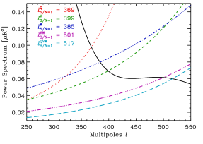
Figure 1: Determination of smoothing FWHM. This is achieved by evaluating the $\ell$-value satisfying the criterion that signal-to-noise is unity ($\rm S/N=1$). The black-solid curve is the WMAP5 best-fitting ‘lcdm+sz+lens’ model power spectrum excluding any correction for pixelization and instrumental beam window functions; the red-dotted, green-dashed, blue-dash-dot, purple-dash-dot-dot, and lightblue-long-dashes curve are averaged noise spectra for the Q, V, W, VW and QVW bands respectively, deconvolved from pixelization and instrumental beams to be consistent with the theoretical power spectrum. The $\ell_{\rm S/N=1}$ values can be determined by the position of the crossing points.

2.5.1 Applied smoothing

Smoothing is applied in our analysis because it enhances the signal-to-noise ratio (S/N) and removes the local sensitivity to the fine-structure of the noise. The angular scale of smoothing is determined by a S/N normalization criterion as shown in Figure  1. For each band, the observed power spectrum, $\tilde{C}_{l}$, is related to the underlying spectrum $C_{l}$, on average, as

$$\langle\tilde{C}_{l}\rangle=b_{l}^{2}p_{l}^{2}C_{l}+\langle N_{l}\rangle,$$ (3)

where $N_{l}$ is the noise power spectrum of each band. We find the $\ell$ values corresponding to ${\rm S/N}=1$, i.e., $C_{l}=b_{l}^{-2}p_{l}^{-2}\langle N_{l}\rangle$, for the Q, V, W, VW and QVW bands, listed in Figure  1. The smoothing suppression factor in $\ell$-space is

$$g(\ell,\theta_{\rm FWHM})=\exp(-\frac{1}{2}\ell(\ell+1)\sigma^{2}),$$ (4)

where $\sigma=\theta_{\rm FWHM}/\sqrt{8\log 2}$, and $\theta_{\rm FWHM}$ is the Gaussian FWHM scale in radians. We choose two different FWHM scales ($\theta_{\rm f1}$ and $\theta_{\rm f2}$) for each band such that $g(l_{\rm S/N=1}^{b},\theta_{\rm f1,f2})=e^{-1},10^{-1}$. The FWHM values for the 5-year S/N normalization are listed in arcmin in Table 1.

Table 1: The Gaussian FWHM scale (arcmin) of all the bands for 5-year S/N normalization.

	Q	V	W	VW	QVW
$\theta_{\rm f1}$	30.984	28.657	29.698	22.828	22.123
$\theta_{\rm f2}$	47.015	43.485	45.064	34.640	33.569

2.5.2 Valid pixels

After smoothing, we are concerned that edge effects due to pixels close to the boundaries of the mask may create artefacts in the local extrema measured in these regions. To solve this problem, we apply the method used by Eriksen et al. (2005). The original mask is convolved with a Gaussian FWHM beam as in Eq.4 and valid pixels for further analysis are defined as those with a value larger than 0.90 in the smoothed mask. We have tested that 0.90 is sufficiently conservative in our local extrema analysis.

2.6 The statistics

In this section, we introduce the statistics by which a comparison will be made between the WMAP 5-year data and simulations, as well as the methodology applied in order to establish confidence levels on these statistics.

2.6.1 One-point statistics

Following the analysis performed by Larson & Wandelt (2004), we calculate the number, mean, variance, skewness and kurtosis value of local extrema. The mean and skewness values of the cold spots are multiplied by $-1$ for convenience when comparing with hotspots. We compute the fraction of simulated statistical values that are lower than those for the WMAP data and use these numbers to make a statement about whether the measurements are consistent with the Gaussian process assumed for the simulations.

To achieve this, we adopt the hypothesis test methodology introduced by Larson & Wandelt (2005), and extensively described in their appendix 2, to establish statistically robust confidence limits for this assessment of our one-point analysis.

As a brief summary of this methodology, consider that we have one number, $x_{0}$, the mean value determined from the observed local extrema, and a sample, $\{x_{i}\}$, from the simulations. We consider the hypothesis ‘$x_{0}$ comes from the same distribution as $\{x_{i}\}$’. If there are $n$ total samples in the simulated ensemble, and $i$ do fall below $x_{0}$, then we can define the quantity $p$ as $i/n$ where $p$ defines the position of $x_{0}$ in the appropriate PDF. We then choose a hypothesis about $p$

$$H:p\in(\alpha/2,1-\alpha/2),$$ (5)

where $\alpha$ is the significance level much less than 1. It is a two-sided hypothesis because $x_{0}$ is less likely to come from the distribution than $\{x_{i}\}$ if it lies on the tail of $\{x_{i}\}$ or beyond, as naturally considered. The frequentist statement is that ‘$H$ is true in a fraction $1-\alpha$ of all possible Gaussian universes’. We make tests for each statistic twice: first, the Type I error (rejection of true hypothesis) probability is controlled to be small; and second, the Type II error (acceptance of the false hypothesis) is controlled. See Appendix 2 of Larson & Wandelt (2005) for comprehensive details.

2.6.2 Two-point statistics

There are two kinds of two-point analysis performed in this paper: the temperature- (T-T) and point- (P-P) angular correlation functions.

The T-T correlation function discussed here has the same definition as that discussed by Eriksen et al. (2005),

$$\xi_{\rm TT}(\theta)=\langle T(\textbf{{n}}_{1})T(\textbf{{n}}_{2})\rangle$$ (6)

where $\cos\theta=\textbf{{n}}_{1}\cdot\textbf{{n}}_{2}$, and the points $\textbf{{n}}_{1}$ and $\textbf{{n}}_{2}$ at which the temperatures are defined correspond to local extrema. We analyse the maxima and minima separately, i.e., only the maxima-maxima ($T_{\rm max}-T_{\rm max}$) and minima-minima ($T_{\rm min}-T_{\rm min}$) correlation functions are evaluated.

The P-P angular correlation function is defined as the excess probability of finding a pair of local extrema at angular separation $\theta$ by direct analogy with the definition used in galaxy distribution studies,

$$dP=\bar{n}[1+\xi_{\rm PP}(\theta)]d\Omega,$$ (7)

where $\bar{n}$ is the mean number density of our sample. The Hamilton estimator of the P-P correlation function is adopted here (Hamilton, 1993),

$$\xi_{\rm PP}(\theta)=\frac{DD(\theta)RR(\theta)}{[DR(\theta)]^{2}}-1,$$ (8)

where $DD(\theta)$ is the number of pairs of local extrema in our data (for either the WMAP observations or a particular simulation) inside the interval $[\theta,\theta+d\theta)$, $RR(\theta)$ is the number of pairs in a random generated sample with separation in the same interval, and $DR(\theta)$ has the same meaning but the pairs are selected between the data and the random sample.

We generate 200000 random points uniformly distributed on the full sphere. We eliminate any adjacent points since these cannot correspond to local extrema as defined in this work. This leaves 135889 surviving points, still at least ten times more numerous than the average number in our data catalog, which is usually considered sufficient for the correlation function study.

$\chi^{2}$ values are computed for both T-T and P-P correlation functions to quantify the degree of agreement between observations and simulations. The $\chi^{2}$ statistic is calculated from the difference between each sample (either observation or simulation) and the average of the simulations on a given scale and defined as

$$\chi^{2}=\sum^{N_{\rm bin}}_{i,j=1}[\xi(i)-\langle\xi(i)\rangle]M^{-1}_{ij}[\xi(j)-\langle\xi(j)\rangle],$$ (9)

where $M^{-1}_{ij}$ is the inverse covariance matrix estimated from the ensemble of correlation functions determined from the Gaussian simulations.

$$M_{ij}=\frac{1}{N_{\rm sim}-1}\sum_{n=1}^{N_{\rm sim}}[\xi_{n}(i)-\langle\xi(i)\rangle][\xi_{n}(j)-\langle\xi(j)\rangle].$$ (10)

where $N_{\rm sim}$ is the total number of simulations.

The $\chi^{2}$ statistic is optimized for studies on CMB $N$-point (especially even-ordered) correlation functions (Eriksen et al., 2004, 2005) since they are strongly asymmetrically distributed. Each 2-point configuration of the full correlation function is transformed by the relation

$$\frac{\rm Rank\ of\ observed\ map}{\rm{Total\ number\ of\ maps}+1}=\frac{1}{\sqrt{2\pi}}\int_{-\infty}^{s}e^{-\frac{1}{2}t^{2}}dt$$ (11)

The numerator of the left hand side is the number of realizations with a lower value than the current one, and the denominator is the total number of realizations plus 1 in order to make $s$ symmetrically distributed around 0 and to avoid an infinite confidence assignment for the largest value. The $\chi^{2}$ value and the covariance matrix are computed from the transformed configurations of the correlation function.

3 RESULTS AND DISCUSSIONS

3.1 One-point results

The one-point statistics establish the shape of the temperature distribution function for local extrema. For example, skewness represents the degree of symmetry between the left and right tails of the probability distribution, and kurtosis measures its ‘peakedness’.

3.1.1 General results

Thousands of simulations are performed for five bands on two smoothing scales with the low-$\ell$ multipoles removed in the range $[0,\ell_{\rm rmv}]$, with $\ell_{\rm rmv}=1,2$. Five kinds of one-point statistic – the number, mean, variance, skewness and kurtosis – of local maxima and minima, are calculated. The frequencies of the simulated statistics lower than the observed values are shown in Table 2 and Table 3. As mentioned in Section 2.6.1, a hypothesis test is performed on each frequency twice, with significance level $\alpha=0.05$. First, the probability of a Type I error is controlled to be as small as $\alpha$, and the frequencies rejected by our test are marked by an asterisk; secondly, we control the probability of a Type II error to be as small as $\alpha$, then the frequencies rejected this time but accepted by the first test are marked by a question mark. For the cases marked by an asterisk, we assert that the data is not consistent with our Gaussian process, with an associated probability $5\%$ of a Type I error.

We ignore the skewness results because no rejection occurs. Tests reject several cases for the number of local extrema, most of which occur on smaller smoothing scales ($\theta_{\rm f1}$) and in the northern hemisphere for cold spots. The mean values are quite consistent with simulations at the $95\%$ confidence level, except for rejections of the W band with $\theta_{\rm f2}$ smoothing in the Galactic northern hemisphere, implying that the cold spots are not cold enough. Other bands with $\theta_{\rm f2}$ smoothing show a similar suppression of cold spots, although the values are accepted by our test.

The main one-point abnormality appears in the variance results. There is also significant hemispherical asymmetry indicated in Table 3 – almost all of the full-sky (NS) and northern (GN and EN) results are strongly rejected for $\ell_{\rm rmv}=1$, as well as GN and most of EN for $\ell_{\rm rmv}=2$. The frequencies with values outside the $3\sigma$ confidence region have been detected and underlined. It is worth noting that the measured variance on the full-sky is more consistent with simulations after quadrupole removal, and also slightly improved for the northern Ecliptic hemisphere, which give us evidence that the observed low-quadrupole is a possible source of such anomalous behaviour, but this may not be the complete explanation.

3.1.2 Residual Galactic foreground

The conventional wisdom suggests that evidence for non-Gaussianity may be associated with residual Galactic foregrounds. We test this simply by imposing additional masks with $|b|<15^{\circ}$, $20^{\circ}$, $25^{\circ}$, $30^{\circ}$ symmetric cuts around the Galactic equator to constrain the one-point statistics. We choose the V band and smoothing scale $\theta_{\rm f2}$ to carry out the test. The maxima and minima in the Galactic-cut region will then not be involved in the conclusions. Table 4 presents the statistics after imposing the Galactic cuts, with monopole and dipole, as well as quadrupole subtraction. Since the skewness is unrevealing, it will not be listed again.

The results are generally similar to the previous cases. In particular, the variance remains as asymmetric as ever. Although in some cases the low-variance improves with increasing Galactic cut, it is difficult to assert whether this is significant. Therefore, it seems unlikely that residual Galactic foregrounds constitute a solution to the anomalies seen in the one-point statistics.

3.1.3 Low-$\ell$ subtraction

Motivated by the quadrupole evidence in Section 3.1.1, we proceed to remove higher moments of $\ell=$ 0–5 and $\ell=$ 0–10 separately from observed and simulated maps on V band. The number, mean, variance and kurtosis of hotspots and cold spots for $\ell_{\rm rmv}=5$ and $\ell_{\rm rmv}=10$ are put in Table 2 and Table 3.

The number, mean and variance show good agreement with simulations for $\ell_{\rm rmv}=5$ and even better for $\ell_{\rm rmv}=10$, but problems of the kurtosis for $\ell_{\rm rmv}=5$ show that the peak of the extrema temperature distribution on ES is much sharper than the Gaussian one, and it disappears after subtraction of the higher moments. This result suggests that the anomalies of the extrema temperature distribution are related to the large-scale moments, especially the first five. However, it is difficult to further confirm how the large-scale moments affect the temperature distribution of local extrema if only the one-point analysis is available. A two-point analysis is necessary, for which we will also investigate the properties of the two-point correlation as a function of different temperature intervals.

Table 2: Frequencies of the extrema one-point statistics derived from simulations with lower values than the WMAP5 data. NS, GN, GS, EN and ES correspond to full-sky, Galactic North, Galactic South, Ecliptic North and Ecliptic South sky-coverage outside KQ75 mask, respectively. $\theta_{\rm f1,f2}$ gives the smoothing scale described by step 2 in Section 2.5. The number 1000, 2000 or 10000 corresponds to how many simulations were performed. The values rejected by the hypothesis test are marked by a * or ?. Frequencies outside the $3\sigma$ confidence region are underlined.

NUMBER	$\ell_{\rm rmv}=1$					$\ell_{\rm rmv}=2$
5yr, KQ75 MASK	NS	GN	GS	EN	ES	NS	GN	GS	EN	ES
Q, max ($\theta_{\rm f1}$,1000)	0.980?	0.894	0.953	0.945	0.943	0.989*	0.852	0.974?	0.937	0.965
Q, min ($\theta_{\rm f1}$,1000)	0.996*	0.989*	0.934	0.983*	0.977?	0.993*	0.986*	0.909	0.973?	0.991*
W, max ($\theta_{\rm f1}$,1000)	0.714	0.577	0.691	0.528	0.641	0.690	0.497	0.789	0.606	0.578
W, min ($\theta_{\rm f1}$,1000)	0.957	0.988*	0.377	0.984*	0.633	0.938	0.990*	0.365	0.986*	0.573
QVW, max ($\theta_{\rm f1}$,1000)	0.922	0.904	0.756	0.924	0.679	0.948	0.793	0.844	0.932	0.671
QVW, min ($\theta_{\rm f1}$,1000)	0.894	0.849	0.723	0.894	0.588	0.847	0.889	0.678	0.905	0.591
V, max ($\theta_{\rm f1}$,2000)	0.8410	0.4940	0.9615	0.8630	0.6435	0.8880	0.2560	0.9695?	0.9045	0.6700
V, min ($\theta_{\rm f1}$,2000)	0.7855	0.8390	0.5585	0.8310	0.6270	0.7535	0.9180	0.3680	0.8110	0.7905
VW, max ($\theta_{\rm f1}$,2000)	0.8995	0.9065	0.6930	0.8980	0.6670	0.9365	0.8355	0.8300	0.9085	0.6490
VW, min ($\theta_{\rm f1}$,2000)	0.7715	0.9735?	0.1860	0.9225	0.4450	0.7490	0.9905*	0.1580	0.9010	0.3775
Q, max ($\theta_{\rm f2}$,1000)	0.889	0.744	0.871	0.959	0.673	0.859	0.654	0.811	0.941	0.600
Q, min ($\theta_{\rm f2}$,1000)	0.908	0.886	0.815	0.880	0.839	0.896	0.869	0.767	0.733	0.855
W, max ($\theta_{\rm f2}$,1000)	0.769	0.468	0.872	0.824	0.679	0.824	0.583	0.883	0.852	0.656
W, min ($\theta_{\rm f2}$,1000)	0.980?	0.996*	0.371	0.973?	0.812	0.966	0.995*	0.333	0.944	0.858
QVW, max ($\theta_{\rm f2}$,1000)	0.766	0.625	0.685	0.788	0.610	0.839	0.410	0.772	0.814	0.675
QVW, min ($\theta_{\rm f2}$,1000)	0.881	0.819	0.769	0.917	0.676	0.821	0.794	0.784	0.880	0.803
V, max ($\theta_{\rm f2}$,10000)	0.5574	0.2597	0.8034	0.5319	0.6107	0.6076	0.2190	0.8228	0.4592	0.6013
V, min ($\theta_{\rm f2}$,10000)	0.9666	0.9618	0.7395	0.9721	0.9073	0.9704	0.9752?	0.6951	0.9657	0.9070
VW, max ($\theta_{\rm f2}$,2000)	0.3810	0.2230	0.5665	0.5890	0.3095	0.3235	0.1395	0.6250	0.5850	0.2025
VW, min ($\theta_{\rm f2}$,2000)	0.7055	0.8150	0.4390	0.8625	0.5105	0.6785	0.8665	0.2880	0.8255	0.6595
	$\ell_{\rm rmv}=5$					$\ell_{\rm rmv}=10$
V, max ($\theta_{\rm f2}$,10000)	0.6932	0.1272	0.9408	0.5051	0.6778	0.6951	0.2259	0.9135	0.3168	0.8733
V, min ($\theta_{\rm f2}$,10000)	0.9001	0.9419	0.5887	0.9264	0.5525	0.8438	0.9132	0.6724	0.8914	0.7488
MEAN	$\ell_{\rm rmv}=1$					$\ell_{\rm rmv}=2$
Q, max ($\theta_{\rm f1}$,1000)	0.332	0.249	0.461	0.498	0.359	0.387	0.414	0.557	0.538	0.252
Q, min ($\theta_{\rm f1}$,1000)	0.132	0.082	0.500	0.256	0.077	0.167	0.044	0.422	0.268	0.064
W, max ($\theta_{\rm f1}$,1000)	0.486	0.237	0.689	0.610	0.515	0.568	0.488	0.785	0.688	0.478
W, min ($\theta_{\rm f1}$,1000)	0.411	0.283	0.728	0.229	0.537	0.476	0.196	0.584	0.247	0.649
QVW, max ($\theta_{\rm f1}$,1000)	0.178	0.057	0.529	0.263	0.236	0.161	0.132	0.631	0.381	0.261
QVW, min ($\theta_{\rm f1}$,1000)	0.503	0.496	0.538	0.247	0.694	0.588	0.509	0.462	0.286	0.775
V, max ($\theta_{\rm f1}$,2000)	0.3925	0.3290	0.4960	0.4475	0.4895	0.4295	0.4230	0.5035	0.4065	0.3590
V, min ($\theta_{\rm f1}$,2000)	0.5445	0.4555	0.6845	0.5205	0.4105	0.6670	0.3950	0.7440	0.6025	0.4270
VW, max ($\theta_{\rm f1}$,2000)	0.4230	0.2385	0.6145	0.3715	0.5690	0.4385	0.3130	0.7485	0.4270	0.5570
VW, min ($\theta_{\rm f1}$,2000)	0.3995	0.2790	0.6950	0.1160	0.7160	0.4540	0.2660	0.6890	0.2130	0.7570
Q, max ($\theta_{\rm f2}$,1000)	0.186	0.203	0.310	0.137	0.322	0.170	0.500	0.234	0.258	0.357
Q, min ($\theta_{\rm f2}$,1000)	0.096	0.095	0.326	0.206	0.082	0.139	0.081	0.484	0.208	0.133
W, max ($\theta_{\rm f2}$,1000)	0.190	0.208	0.376	0.344	0.222	0.175	0.478	0.351	0.424	0.209
W, min ($\theta_{\rm f2}$,1000)	0.065	0.014*	0.441	0.055	0.140	0.082	0.006*	0.493	0.049	0.234
QVW, max ($\theta_{\rm f2}$,1000)	0.309	0.111	0.624	0.305	0.517	0.338	0.366	0.624	0.392	0.523
QVW, min ($\theta_{\rm f2}$,1000)	0.161	0.101	0.407	0.167	0.304	0.260	0.108	0.530	0.278	0.364
V, max ($\theta_{\rm f2}$,10000)	0.1653	0.1369	0.3753	0.1999	0.3296	0.1638	0.4857	0.4187	0.3162	0.2739
V, min ($\theta_{\rm f2}$,10000)	0.1066	0.0769	0.3814	0.1181	0.1713	0.1509	0.0425	0.4078	0.1352	0.1719
VW, max ($\theta_{\rm f2}$,2000)	0.2980	0.1280	0.7070	0.4125	0.4245	0.3790	0.2320	0.7705	0.5585	0.3730
VW, min ($\theta_{\rm f2}$,2000)	0.2790	0.0880	0.6940	0.2050	0.3485	0.3215	0.0475	0.7790	0.2455	0.5065
	$\ell_{\rm rmv}=5$					$\ell_{\rm rmv}=10$
V, max ($\theta_{\rm f2}$,10000)	0.4486	0.6654	0.2473	0.3489	0.2955	0.4703	0.4729	0.3356	0.6542	0.2627
V, min ($\theta_{\rm f2}$,10000)	0.0720	0.0339	0.3632	0.1334	0.1788	0.1100	0.1764	0.4261	0.1804	0.1273

Table 3: Continued from Table 2

VARIANCE	$\ell_{\rm rmv}=1$					$\ell_{\rm rmv}=2$
5yr, KQ75 MASK	NS	GN	GS	EN	ES	NS	GN	GS	EN	ES
Q, max ($\theta_{\rm f1}$,1000)	0.006*	0.013*	0.382	0.006*	0.248	0.063	0.005*	0.683	0.017*	0.541
Q, min ($\theta_{\rm f1}$,1000)	0.006*	0.002*	0.482	0.005*	0.325	0.077	0.004*	0.851	0.030?	0.629
W, max ($\theta_{\rm f1}$,1000)	0.002*	0.011*	0.233	0.003*	0.187	0.018?	0.006*	0.507	0.007*	0.444
W, min ($\theta_{\rm f1}$,1000)	0.001*	0.001*	0.433	0.003*	0.226	0.027?	0.000*	0.773	0.016*	0.456
QVW, max ($\theta_{\rm f1}$,1000)	0.007*	0.018?	0.339	0.006*	0.276	0.077	0.018?	0.667	0.024?	0.572
QVW, min ($\theta_{\rm f1}$,1000)	0.002*	0.001*	0.474	0.003*	0.238	0.027?	0.000*	0.790	0.013*	0.524
V, max ($\theta_{\rm f1}$,2000)	0.0030*	0.0090*	0.3035	0.0035*	0.2170	0.0340	0.0075*	0.6415	0.0110*	0.5200
V, min ($\theta_{\rm f1}$,2000)	0.0045*	0.0015*	0.4265	0.0025*	0.2335	0.0520	0.0010*	0.7495	0.0235?	0.5815
VW, max ($\theta_{\rm f1}$,2000)	0.0010*	0.0060*	0.2445	0.0015*	0.1795	0.0220?	0.0035*	0.5360	0.0060*	0.4250
VW, min ($\theta_{\rm f1}$,2000)	0.0025*	0.0010*	0.3660	0.0040*	0.1715	0.0320	0.0000*	0.6830	0.0160*	0.4530
Q, max ($\theta_{\rm f2}$,1000)	0.009*	0.004*	0.494	0.003*	0.359	0.082	0.005*	0.813	0.011*	0.688
Q, min ($\theta_{\rm f2}$,1000)	0.006*	0.003*	0.478	0.003*	0.337	0.053	0.001*	0.807	0.021?	0.613
W, max ($\theta_{\rm f2}$,1000)	0.005*	0.007*	0.353	0.003*	0.308	0.050	0.003*	0.662	0.010*	0.591
W, min ($\theta_{\rm f2}$,1000)	0.007*	0.002*	0.465	0.004*	0.300	0.048	0.001*	0.810	0.022?	0.566
QVW, max ($\theta_{\rm f2}$,1000)	0.003*	0.006*	0.358	0.003*	0.227	0.021?	0.004*	0.644	0.011*	0.515
QVW, min ($\theta_{\rm f2}$,1000)	0.005*	0.001*	0.510	0.002*	0.338	0.057	0.000*	0.846	0.018?	0.648
V, max ($\theta_{\rm f2}$,10000)	0.0040*	0.0021*	0.4491	0.0009*	0.3188	0.0564	0.0031*	0.7875	0.0059*	0.6949
V, min ($\theta_{\rm f2}$,10000)	0.0028*	0.0011*	0.4345	0.0009*	0.2750	0.0343	0.0013*	0.8188	0.0061*	0.5911
VW, max ($\theta_{\rm f2}$,2000)	0.0055*	0.0105*	0.3425	0.0035*	0.2425	0.0465	0.0090*	0.5935	0.0080*	0.5040
VW, min ($\theta_{\rm f2}$,2000)	0.0065*	0.0025*	0.4445	0.0015*	0.3110	0.0630	0.0025*	0.7925	0.0155*	0.6145
	$\ell_{\rm rmv}=5$					$\ell_{\rm rmv}=10$
V, max ($\theta_{\rm f2}$,10000)	0.0808	0.0716	0.6817	0.0443	0.4864	0.0953	0.2413	0.2928	0.2689	0.3853
V, min ($\theta_{\rm f2}$,10000)	0.1213	0.0342	0.6285	0.0229?	0.4688	0.0463	0.1644	0.2450	0.1584	0.3040
KURTOSIS	$\ell_{\rm rmv}=1$					$\ell_{\rm rmv}=2$
Q, max ($\theta_{\rm f1}$,1000)	0.247	0.373	0.104	0.195	0.532	0.231	0.259	0.327	0.082	0.648
Q, min ($\theta_{\rm f1}$,1000)	0.515	0.140	0.575	0.290	0.824	0.752	0.062	0.884	0.309	0.820
W, max ($\theta_{\rm f1}$,1000)	0.567	0.755	0.254	0.642	0.608	0.643	0.596	0.479	0.559	0.724
W, min ($\theta_{\rm f1}$,1000)	0.716	0.613	0.465	0.493	0.804	0.800	0.382	0.675	0.493	0.847
QVW, max ($\theta_{\rm f1}$,1000)	0.645	0.861	0.221	0.756	0.621	0.741	0.732	0.660	0.715	0.821
QVW, min ($\theta_{\rm f1}$,1000)	0.735	0.579	0.560	0.571	0.791	0.818	0.234	0.756	0.435	0.913
V, max ($\theta_{\rm f1}$,2000)	0.7010	0.9090	0.2355	0.7250	0.6925	0.8130	0.8690	0.6605	0.7105	0.8420
V, min ($\theta_{\rm f1}$,2000)	0.7055	0.6930	0.4000	0.6395	0.7935	0.8015	0.4760	0.6505	0.6335	0.8845
VW, max ($\theta_{\rm f1}$,2000)	0.4770	0.7145	0.1925	0.6290	0.5885	0.6125	0.5700	0.6410	0.6430	0.7670
VW, min ($\theta_{\rm f1}$,2000)	0.6050	0.6375	0.3105	0.5475	0.6420	0.6560	0.2700	0.4720	0.4250	0.7020
Q, max ($\theta_{\rm f2}$,1000)	0.742	0.826	0.382	0.824	0.693	0.801	0.719	0.642	0.781	0.846
Q, min ($\theta_{\rm f2}$,1000)	0.440	0.700	0.085	0.482	0.598	0.682	0.363	0.437	0.520	0.756
W, max ($\theta_{\rm f2}$,1000)	0.822	0.850	0.604	0.897	0.784	0.890	0.715	0.733	0.881	0.845
W, min ($\theta_{\rm f2}$,1000)	0.881	0.942	0.381	0.579	0.932	0.932	0.774	0.642	0.615	0.942
QVW, max ($\theta_{\rm f2}$,1000)	0.477	0.483	0.264	0.536	0.533	0.514	0.390	0.569	0.454	0.668
QVW, min ($\theta_{\rm f2}$,1000)	0.705	0.584	0.424	0.514	0.811	0.800	0.304	0.646	0.483	0.911
V, max ($\theta_{\rm f2}$,10000)	0.8272	0.8613	0.5090	0.7485	0.8380	0.8448	0.7720	0.6555	0.6487	0.8630
V, min ($\theta_{\rm f2}$,10000)	0.8999	0.9194	0.5643	0.8362	0.8908	0.9741?	0.8131	0.8130	0.8565	0.9359
VW, max ($\theta_{\rm f2}$,2000)	0.5245	0.6395	0.2705	0.4855	0.6195	0.5710	0.4900	0.6170	0.4370	0.8310
VW, min ($\theta_{\rm f2}$,2000)	0.7000	0.6475	0.4175	0.4475	0.8770	0.8170	0.4605	0.5855	0.4135	0.9170
	$\ell_{\rm rmv}=5$					$\ell_{\rm rmv}=10$
V, max ($\theta_{\rm f2}$,10000)	0.9663	0.6138	0.9147	0.2776	0.9833*	0.6631	0.5874	0.5407	0.2317	0.9339
V, min ($\theta_{\rm f2}$,10000)	0.9909*	0.7515	0.9754?	0.6519	0.9864*	0.9728?	0.8389	0.8678	0.7187	0.9685

Table 4: One-point statistics as a function of the Galactic cut, $|b|=15^{\circ}$, $20^{\circ}$, $25^{\circ}$ and $30^{\circ}$, imposed in addition to the KQ75 mask for $\ell_{\rm rmv}=1$ and $2$. 10000 simulations were performed for V band, with smoothing $\rm{FWHM}=43.485^{\prime}$.

	$\ell_{\rm rmv}=1$					$\ell_{\rm rmv}=2$
$|b|$(degree)	NS	GN	GS	EN	ES	NS	GN	GS	EN	ES
NUM(max) 15	0.5818	0.3038	0.7204	0.4550	0.6224	0.5521	0.3483	0.8076	0.3983	0.6242
20	0.4414	0.3606	0.5036	0.3480	0.5576	0.4110	0.4099	0.6079	0.2775	0.5359
25	0.4747	0.3329	0.5817	0.3205	0.5952	0.4183	0.3706	0.6329	0.2659	0.5143
30	0.3189	0.2562	0.4371	0.2720	0.3507	0.2365	0.2598	0.4745	0.2055	0.2871
NUM(min) 15	0.9839*	0.9672	0.8194	0.9849*	0.9280	0.9827*	0.9712	0.7839	0.9791*	0.9127
20	0.9932*	0.9902*	0.8124	0.9935*	0.9557	0.9938*	0.9931*	0.7843	0.9911*	0.9361
25	0.9802*	0.9812*	0.7173	0.9832*	0.9322	0.9855*	0.9840*	0.7055	0.9814*	0.9264
30	0.9156	0.9917*	0.3048	0.9731?	0.7751	0.9379	0.9952*	0.2802	0.9733?	0.7995
MEAN(max) 15	0.1553	0.0507	0.3109	0.1326	0.2744	0.0666	0.5647	0.5054	0.1618	0.1535
20	0.3028	0.0924	0.3289	0.1662	0.4353	0.1026	0.7123	0.5231	0.1505	0.3231
25	0.4125	0.1132	0.4237	0.2434	0.4702	0.1462	0.5455	0.6947	0.2206	0.3787
30	0.4713	0.1369	0.4425	0.2914	0.4812	0.1585	0.3582	0.5935	0.2892	0.3596
MEAN(min) 15	0.4629	0.6680	0.3954	0.4417	0.4593	0.6154	0.0837	0.2139	0.4418	0.5819
20	0.4863	0.6534	0.5305	0.5805	0.4183	0.6997	0.0354	0.3214	0.5704	0.5198
25	0.4539	0.6290	0.4977	0.6005	0.3845	0.6756	0.0681	0.2671	0.5768	0.4469
30	0.4520	0.5258	0.6342	0.5708	0.4604	0.7103	0.1645	0.6419	0.5195	0.5961
VAR(max) 15	0.0028*	0.0006*	0.4936	0.0005*	0.3152	0.0460	0.0017*	0.7935	0.0023*	0.6481
20	0.0033*	0.0014*	0.4748	0.0010*	0.3046	0.0493	0.0024*	0.7675	0.0039*	0.6652
25	0.0027*	0.0028*	0.3957	0.0028*	0.1961	0.0409	0.0027*	0.6755	0.0050*	0.5817
30	0.0020*	0.0042*	0.2589	0.0010*	0.1514	0.0195*	0.0037*	0.5766	0.0022*	0.5319
VAR(min) 15	0.0013*	0.0006*	0.3974	0.0005*	0.2368	0.0183*	0.0013*	0.7396	0.0015*	0.5043
20	0.0019*	0.0011*	0.4116	0.0009*	0.2532	0.0235?	0.0012*	0.7340	0.0024*	0.5714
25	0.0023*	0.0020*	0.3898	0.0032*	0.1640	0.0207*	0.0014*	0.7382	0.0063*	0.5098
30	0.0026*	0.0029*	0.3302	0.0020*	0.1716	0.0176*	0.0020*	0.7049	0.0040*	0.5517
KURT(max) 15	0.8411	0.8573	0.5413	0.7013	0.8641	0.8571	0.7929	0.7216	0.6022	0.9074
20	0.7587	0.8111	0.4698	0.6584	0.7888	0.7785	0.7396	0.6777	0.5720	0.8724
25	0.7332	0.8665	0.3666	0.6614	0.8423	0.7816	0.8404	0.7091	0.6413	0.9210
30	0.6148	0.8270	0.3273	0.5461	0.7880	0.6786	0.7711	0.7072	0.4947	0.8280
KURT(min) 15	0.8666	0.8631	0.6038	0.7742	0.8656	0.9641	0.8418	0.8050	0.7753	0.9310
20	0.8556	0.8654	0.5891	0.6777	0.9060	0.9526	0.8694	0.7891	0.7309	0.9439
25	0.7774	0.7677	0.5720	0.5745	0.8959	0.9048	0.6792	0.7995	0.6469	0.9033
30	0.8698	0.8064	0.7411	0.7471	0.9221	0.9510	0.7932	0.8945	0.8110	0.9146

Table 5: Continued from Table 4 with $\ell_{\rm rmv}=5$ and $10$.

	$\ell_{\rm rmv}=5$					$\ell_{\rm rmv}=10$
$|b|$(degree)	NS	GN	GS	EN	ES	NS	GN	GS	EN	ES
NUM(max) 15	0.7432	0.2372	0.9537	0.4920	0.7149	0.7470	0.3177	0.9212	0.3593	0.9189
20	0.6206	0.3685	0.7804	0.3241	0.6494	0.6891	0.3648	0.8352	0.3061	0.8972
25	0.6084	0.3158	0.7905	0.2675	0.6004	0.6783	0.4069	0.8071	0.3005	0.8891
30	0.3821	0.2499	0.5695	0.1833	0.3841	0.3867	0.3080	0.5927	0.2512	0.6930
NUM(min) 15	0.9378	0.9597	0.6160	0.9598	0.6016	0.8918	0.9318	0.7042	0.9262	0.7854
20	0.9674	0.9822*	0.6840	0.9779*	0.6868	0.9574	0.9796*	0.7329	0.9462	0.8530
25	0.9498	0.9755?	0.6276	0.9531	0.6514	0.9375	0.9682	0.6480	0.8907	0.8752
30	0.8915	0.9885*	0.2275	0.9234	0.3993	0.8764	0.9882*	0.3297	0.8783	0.6698
MEAN(max) 15	0.3757	0.5227	0.2834	0.2356	0.3585	0.4453	0.4188	0.4247	0.6438	0.2208
20	0.4934	0.6329	0.3103	0.2488	0.5865	0.4512	0.6615	0.2511	0.5414	0.3296
25	0.7283	0.6669	0.6404	0.5735	0.7172	0.6779	0.5447	0.5576	0.6904	0.5320
30	0.7607	0.6678	0.6307	0.7316	0.6048	0.6975	0.4704	0.5787	0.7336	0.4436
MEAN(min) 15	0.2167	0.1231	0.3206	0.2959	0.2545	0.1851	0.2985	0.3055	0.2505	0.2442
20	0.2078	0.0765	0.4253	0.3014	0.1706	0.1919	0.1318	0.5056	0.2762	0.1873
25	0.0705	0.0318	0.2508	0.1136	0.0786	0.0767	0.1317	0.2935	0.2037	0.0598
30	0.0898	0.0223*	0.5859	0.0642	0.3915	0.1743	0.1343	0.6256	0.1912	0.3039
VAR(max) 15	0.1011	0.0597	0.7851	0.0533	0.5263	0.1112	0.1893	0.3943	0.2894	0.4045
20	0.1124	0.0637	0.7398	0.0501	0.4753	0.0984	0.1415	0.3727	0.3446	0.3012
25	0.0822	0.0420	0.5815	0.0352	0.3717	0.0595	0.1208	0.2426	0.2619	0.1737
30	0.0588	0.0391	0.4834	0.0225?	0.4489	0.0604	0.2150	0.1922	0.2931	0.2051
VAR(min) 15	0.1020	0.0385	0.6171	0.0192*	0.5127	0.0246?	0.1240	0.1634	0.1131	0.2558
20	0.1183	0.0285	0.6540	0.0195*	0.5278	0.0261?	0.0606	0.2471	0.1367	0.2534
25	0.1547	0.0230?	0.7443	0.0423	0.4741	0.0466	0.0667	0.3211	0.2351	0.1873
30	0.1752	0.0260?	0.7560	0.0294	0.6663	0.1199	0.1905	0.4644	0.3255	0.3856
KURT(max) 15	0.9673	0.6796	0.8800	0.2059	0.9888*	0.6835	0.6629	0.4533	0.2227	0.9488
20	0.9756?	0.6771	0.9253	0.2814	0.9913*	0.6926	0.6320	0.5131	0.2714	0.9477
25	0.9882*	0.8077	0.9453	0.3999	0.9950*	0.7609	0.7060	0.5327	0.3122	0.9657
30	0.9495	0.4888	0.9208	0.3806	0.9672	0.5898	0.5610	0.4905	0.3529	0.9347
KURT(min) 15	0.9948*	0.7858	0.9848*	0.6574	0.9907*	0.9859*	0.8352	0.9078	0.7469	0.9780*
20	0.9951*	0.8475	0.9819*	0.5897	0.9956*	0.9841*	0.8354	0.8896	0.6954	0.9844*
25	0.9859*	0.7030	0.9786*	0.5293	0.9904*	0.9487	0.6758	0.8421	0.5825	0.9551
30	0.9927*	0.7418	0.9887*	0.6970	0.9885*	0.8970	0.5917	0.7800	0.6058	0.8987

3.2 Two-point results

We study the correlation functions of hot and cold spots for the V-band in five sky coverages with three kinds of temperature threshold applied – no threshold ($\rm T_{max}>-\infty$, $\rm T_{min}<\infty$), $1\sigma_{\rm sky}$ ($\rm T_{max}>1\sigma_{\rm sky}$ , $\rm T_{min}<-1\sigma_{\rm sky}$) and $2\sigma_{\rm sky}$ ($\rm T_{max}>2\sigma_{\rm sky}$, $\rm T_{min}<-2\sigma_{\rm sky}$), where $\sigma_{\rm sky}$ is the standard deviation of the temperature of all the valid pixels in a certain sky region. For the sky region outside the KQ75 mask, we compute correlation functions from $0^{\circ}$ to $180^{\circ}$, divided into 1000 bins, and from $0^{\circ}$ to $90^{\circ}$ with 500 bins for the four hemispheres in question, since in these cases pairs with separations larger than $90^{\circ}$ are so rare, in particular for the 2$\sigma_{\rm sky}$ threshold, that the correlation functions become strongly oscillatory, affecting the accuracy of inversion of the covariance matrix.

Large-scale modes do affect the confidence level of our one-point statistics, especially the variance, the temperature-temperature correlation of local extrema at zero lag. Thus, conceivably, such a low-$\ell$ subtraction is also of importance to the correlation study. According to the theoretical calculation of T-T correlation by Heavens & Sheth (1999), there are oscillation features on angular scales from 10 to 100 arcmin, however, we will not attempt to investigate these features because of the observational resolution and smoothing procedure during the data processing. We expect stronger signal in this angular range by the forthcoming higher resolution full-sky CMB survey, the PLANCK mission.

3.2.1 T-T correlation

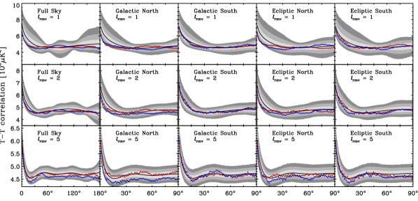
Figure 2: Temperature-temperature correlation functions of hotspots and cold spots without temperature threshold, for five sky-coverages adopted in this paper. The red (blue) dots correspond to the correlation function bins of hotspots (cold spots) observed in the WMAP V-band data. The light, middle and dark gray shaded bands show, respectively, the 68.26%, 95.44% and 99.74% confidence regions determined from 10000 MC simulations, and the black solid line shows the median. Since the statistical bands of hotspots and cold spots are quite identical, we plot averaged bands here. The correlation functions on both full sky and hemispheres are rebinned to 100 bins.

We show the temperature-temperature correlation functions without threshold applied in Figure 2. The correlation functions have been rebinned to 100 bins for both full sky and hemispheres and the first bins are dropped.

Spergel et al. (2003) and Copi et al. (2008) report a lack of correlated signal compared to the $\Lambda$CDM model for angular scales greater than $60^{\circ}$ for WMAP1 and WMAP5, respectively. However, as shown by the top and middle panels of Figure 3, there is no significant lack of correlation for the hot and cold spots on corresponding scales, when computed on either the full-sky or hemispheres. However, what is of note is the lack of variance in the bins on these angular scales – almost all lie within the $2\sigma$ confidence region. In fact, the correlation properties of the hot and cold spots show several interesting properties as a function of angular scale and temperature threshold, as we discuss below.

In the case of the full sky analysis with $\ell_{\rm rmv}=1$ and without any threshold applied, it should be apparent that there is a strong suppression of the correlation function for the bins of both hot and cold spots on scales less than about $20^{\circ}$ (corresponding to the typical scale of $\ell=10$), to amplitudes around or even below the lower limit of the Gaussian $3\sigma$ confidence region. Similar behaviour is seen on scales less than $10^{\circ}$ in the Galactic and Ecliptic north ($\ell_{\rm rmv}=1$), whereas the southern sky shows quite a good agreement with theoretical expectations. This corresponds to a hemispherical asymmetry of power seen in the fluctuations of local extrema. The suppression still exists after quadrupole subtraction, in particular the correlation of cold spots in the Galactic north is lower than the $3\sigma$ confidence region at small scales. After removing the modes for $\ell_{\rm rmv}=5$ and $10$, the small-scale suppression become less significant and the hotspots correlation shows perfect agreement with the median, especially on the full-sky, which gives strong and self-consistent evidence that large-scale moments ($\ell\leq 10$) affect the small-scale temperature-correlation of local extrema. Notice that the distribution of correlations becomes less structured on large-scale if higher moments are subtracted.

The angular structure of correlations for hot spots and cold spots should be identical in theory, but the discrepancy between them gets larger as higher moments are removed on both the full-sky and two northern hemispheres. The hotspots are quite consistent with the median of the predicted curves, whereas the cold spots on NS, GN and EN are less correlated in the cases $\ell_{\rm rmv}=5$ and 10.

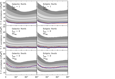
Figure 3: Temperature-temperature correlation functions of hotspots and cold spots valid for thresholds (1$\sigma_{\rm sky}$ and $2\sigma_{\rm sky}$). The nomenclature of the dots and bands follows the same style as Figure 2.

The application of temperature thresholds to the set of hot and cold spots included in the correlation study is also revealing (Figure 3). There are strong suppressions on the full-sky and northern hemispheres at all scales if the $1\sigma_{\rm sky}$ or $2\sigma_{\rm sky}$ threshold is applied. For $\ell_{\rm rmv}=1$ and 2 on GN and EN, most bins are suppressed to the lower limit of $3\sigma$ confidence region, and many are apparently under the lower limit of the $3\sigma$ confidence region defined by simulations. Conversely, results for the southern sky still indicate agreement with the best-fitting cosmological model. However, it should be recognised that, apart from an overall scale-factor, the detailed shape of the observed point-sets is consistent with the median at all other scales. This implies that the T-T properties arise not from an anomalous spatial clustering (or anti-clustering of local extrema), but as a consequence of the statistical nature of the observed temperature distribution. Specifically, it is conceivable that the local extrema with higher temperatures in the northern sky are not extreme enough.

Investigation of the corresponding cases for the P-P correlation function should then also prove revealing.

We calculate the $\chi^{2}_{s}$ value defined by Eq.9 based on the transformed distribution of the correlation functions to quantify the degree of agreement between the observed data and our Gaussian simulations. The fractions of simulations with $\chi^{2}_{s}$ value lower than observed are listed in Table 6, with those larger than 0.975 underlined. All the values after $\ell_{\rm rmv}=10$ become normal. Notice that there are cases with very low $p$-values, implying very, in some cases overly, good agreement with the median. The disagreement of the small-scale correlation without an applied threshold on full-sky coverage cannot be distinguished by this full-scale analysis, and additional small-scale analysis is necessary.

Table 6: The frequencies of $\chi^{2}_{s}$ values from simulations with lower amplitude than the WMAP data as determined for the transformed T-T correlation functions. The values higher than 0.9750 are underlined to demonstrate rejection of the Gaussian hypothesis at $2\sigma$ level.

$\chi^{2}_{s}(TT)$-frequencies	$\ell_{\rm rmv}=1$					$\ell_{\rm rmv}=2$
Thresholds	NS	GN	GS	EN	ES	NS	GN	GS	EN	ES
$\rm T_{max}>-\infty$	0.5774	0.9156	0.0077	0.6503	0.1141	0.5379	0.5070	0.0942	0.5199	0.0375
$\rm T_{min}<\infty$	0.7595	0.7728	0.1413	0.7883	0.2150	0.4973	0.9488	0.0672	0.5863	0.2967
$\rm T_{max}>1\sigma_{\rm sky}$	0.9958	0.9947	0.1553	0.9994	0.4059	0.9219	0.9968	0.4824	0.9983	0.2031
$\rm T_{min}<-1\sigma_{\rm sky}$	0.9947	0.9991	0.2315	0.9973	0.3624	0.9470	0.9944	0.4083	0.9892	0.1161
$\rm T_{max}>2\sigma_{\rm sky}$	0.9919	0.9795	0.3493	0.9955	0.4131	0.8506	0.9739	0.5942	0.9746	0.5306
$\rm T_{min}<-2\sigma_{\rm sky}$	0.9815	0.9928	0.0575	0.9973	0.0627	0.7562	0.9887	0.6556	0.9916	0.6736
	$\ell_{\rm rmv}=5$					$\ell_{\rm rmv}=10$
$\rm T_{max}>-\infty$	0.0962	0.2958	0.1807	0.3249	0.2915	0.0233	0.0473	0.1605	0.1377	0.4012
$\rm T_{min}<\infty$	0.8520	0.9400	0.2723	0.8133	0.5824	0.7731	0.7038	0.1791	0.6973	0.7379
$\rm T_{max}>1\sigma_{\rm sky}$	0.8714	0.9628	0.2982	0.9862	0.0029	0.8287	0.7957	0.0259	0.6694	0.0186
$\rm T_{min}<-1\sigma_{\rm sky}$	0.9394	0.8610	0.2107	0.9732	0.2949	0.9505	0.6467	0.4162	0.7179	0.5368
$\rm T_{max}>2\sigma_{\rm sky}$	0.7214	0.7034	0.3321	0.9540	0.5583	0.7839	0.3833	0.5271	0.1774	0.4144
$\rm T_{min}<-2\sigma_{\rm sky}$	0.7261	0.8316	0.4718	0.8683	0.1474	0.8029	0.7024	0.0438	0.7411	0.4075

3.2.2 P-P correlation

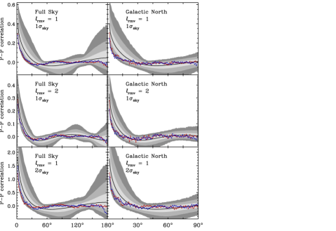
Figure 4: Point-point correlation functions of hotspots and cold spots valid for thresholds (1$\sigma_{\rm sky}$ and $2\sigma_{\rm sky}$). 5000 simulations are performed. The nomenclature of the dots and bands follows the same style as Figure 2.

The spatial clustering of local extrema quantified by the P-P correlation function is analysed by comparing with 5000 simulations. This analysis is also based on V-band data with a $43.485^{\prime}$ FWHM Gaussian beam smoothing applied. As with the temperature correlation, we rebin the original structure to 100 bins for both full sky and hemispheres and drop the first bins. Temperature thresholds are also applied to select the valid spots, but only their spatial positions are taken into account. Some of the results are plotted in Figure 4. We take the simple averaged confidence regions for hotspots and cold spots since the profiles of these two are again essentially identical.

We do not show results corresponding to the application of no threshold since the observed structure is trivial, essentially a scatter around zero over all separation angles, and no high-significance results are found under these conditions. This means that the extrema in our data set are nearly-uniformly distributed on the sphere. Instead, we focus on the correlation structure of valid spots as a function of temperature thresholds. We expect stronger clustering if we introduce a certain level threshold that retains only higher amplitude peaks. We also introduce the notion of a ‘clustering scale’ by analogy with studies of the galaxy two-point correlation function, The first decline to zero amplitude defines the characteristic radius of an extended hot or cold region (or ‘cluster’) and bumps on larger scales reflect the correlation among ‘clusters’. Since the major clustering regions are determined by large-scale modes, and the local extrema created by other modes in these regions can be enhanced or suppressed by a certain level, the features of the CMB local extrema correlation functions (both T-T and P-P) represent the magnitude and scale of the hot and cold regions of large-scale modes.

The results are consistent with our expectations. The positive-valued structure demonstrates an approximate $30^{\circ}$ typical clustering scale before removing the quadrupole, and valid points for the $2\sigma_{\rm sky}$ threshold show a much stronger clustering amplitude (the left-three panels of Figure 4). Moreover, the curves decline to zero faster after more moments are removed, and are less structured on larger angular separations because there is no sufficiently-long wavelength fluctuation to correlate the local extrema on these scales. Thus, this typical clustering scale corresponds to the spatial pattern of large-scale modes.

There is a $3\sigma$-level suppression for both $1\sigma_{\rm sky}$ thresholded hot and cold spot correlations on scales less than $20^{\circ}$ as computed for the full sky and $\ell_{\rm rmv}=1$, and an approximately $2\sigma$-level suppression for the $2\sigma_{\rm sky}$ threshold, resulting from the less correlated northern sky. After the first 5 or 10, moments are removed, better consistency with the simulations is again seen yielding additional evidence that the abnormal properties of the large angular-scale temperature structure affects the statistical properties of our observed sky.

Table 7: The frequencies of $\chi^{2}_{s}$ values from our simulations with amplitudes lower than the WMAP data for the transformed P-P correlation functions.

$\chi^{2}_{s}(PP)$-frequencies	$\ell_{\rm rmv}=1$					$\ell_{\rm rmv}=2$
Thresholds	NS	GN	GS	EN	ES	NS	GN	GS	EN	ES
$\rm T_{max}>-\infty$	0.2896	0.8154	0.2632	0.5712	0.7857	0.1993	0.7161	0.2228	0.6309	0.7139
$\rm T_{min}<\infty$	0.4936	0.2940	0.5508	0.0260	0.8302	0.3725	0.0458	0.3352	0.0055	0.6782
$\rm T_{max}>1\sigma_{\rm sky}$	0.9139	0.7250	0.3310	0.8926	0.6794	0.4111	0.7817	0.5479	0.5460	0.4217
$\rm T_{min}<-1\sigma_{\rm sky}$	0.8601	0.8479	0.1380	0.9190	0.5717	0.5655	0.8608	0.6618	0.3590	0.6761
$\rm T_{max}>2\sigma_{\rm sky}$	0.9075	0.6543	0.4716	0.7523	0.7584	0.6277	0.6851	0.2454	0.5536	0.1664
$\rm T_{min}<-2\sigma_{\rm sky}$	0.7554	0.5749	0.0364	0.8834	0.3955	0.0878	0.7157	0.7559	0.2125	0.6901
	$\ell_{\rm rmv}=5$					$\ell_{\rm rmv}=10$
$\rm T_{max}>-\infty$	0.4964	0.8852	0.0597	0.7042	0.7577	0.2212	0.9706	0.2468	0.6877	0.8827
$\rm T_{min}<\infty$	0.3305	0.0296	0.1814	0.0083	0.7874	0.2064	0.1126	0.3476	0.0156	0.8086
$\rm T_{max}>1\sigma_{\rm sky}$	0.4998	0.7692	0.3950	0.6966	0.0114	0.3355	0.9616	0.1350	0.7969	0.2687
$\rm T_{min}<-1\sigma_{\rm sky}$	0.4470	0.6074	0.9161	0.7757	0.6521	0.5145	0.4639	0.6108	0.6913	0.7653
$\rm T_{max}>2\sigma_{\rm sky}$	0.1050	0.2946	0.0795	0.5207	0.5148	0.1550	0.3517	0.0167	0.7053	0.1376
$\rm T_{min}<-2\sigma_{\rm sky}$	0.2703	0.8831	0.7519	0.5813	0.0762	0.1392	0.4512	0.8849	0.5299	0.8398

Table 7 lists the frequency for which the $\chi^{2}_{s}$ values computed for the simulations are lower than the observed WMAP values for the transformed P-P correlation functions. No rejection is detected, supporting the consistency of the spatial distribution of the observed local extrema with our Gaussian simulations, over the whole angular range of our concern, while suppression on small-scales is not revealed by this analysis.

3.2.3 Analysis on small scales

Both the T-T (no threshold) and P-P (thresholded) correlation functions record a $3\sigma$-level suppression on scales less than $20^{\circ}$ for the full sky and $10^{\circ}$ for northern hemispheres. Tojeiro et al. (2006) find evidence for non-Gaussianity using the P-P correlation function of local extrema in WMAP1 data. The correlation function they use is estimated and rebinned to 19 equally spaced bins up to a maximum separation of $30^{\circ}$. To make a comparison with their results, we analyse the $\chi^{2}_{s}$-frequency of rebinned T-T and P-P correlations on scales less than $30^{\circ}$ with the first 17 bins for the full sky and on scales less than $15^{\circ}$ with first 9 bins for the hemispheres.

Table 8: $\chi^{2}_{s}$-frequency for T-T (no threshold) and P-P (thresholds) correlations on small angular scales, up to the maximum separation of $30^{\circ}$ for full sky and $15^{\circ}$ for hemispheres.

$\chi^{2}_{s}$-fractions	$\ell_{\rm rmv}=1$					$\ell_{\rm rmv}=2$
Thresholds	NS	GN	GS	EN	ES	NS	GN	GS	EN	ES
$\rm T^{TT}_{max}>-\infty$	0.9527	0.9980	0.3425	0.9968	0.5120	0.8982	0.9682	0.3055	0.9828	0.2511
$\rm T^{TT}_{min}<\infty$	0.9682	0.9968	0.0788	0.9936	0.6851	0.8026	0.9994	0.5489	0.9674	0.3035
$\rm T^{PP}_{max}>1\sigma_{\rm sky}$	0.9851	0.9806	0.0384	0.9944	0.4503	0.7419	0.9851	0.6912	0.9657	0.3813
$\rm T^{PP}_{min}<-1\sigma_{\rm sky}$	0.9643	0.9986	0.1756	0.9825	0.4230	0.7369	0.9946	0.7110	0.9570	0.2748
$\rm T^{PP}_{max}>2\sigma_{\rm sky}$	0.9850	0.9351	0.6916	0.9894	0.6918	0.7164	0.9696	0.5238	0.9599	0.2122
$\rm T^{PP}_{min}<-2\sigma_{\rm sky}$	0.8410	0.9509	0.0518	0.9768	0.2010	0.3378	0.9702	0.5541	0.8320	0.2622
	$\ell_{\rm rmv}=5$					$\ell_{\rm rmv}=10$
$\rm T^{TT}_{max}>-\infty$	0.1885	0.3167	0.0529	0.8406	0.2342	0.2272	0.4377	0.4106	0.0645	0.5216
$\rm T^{TT}_{min}<\infty$	0.9002	0.9934	0.2804	0.9226	0.2513	0.8145	0.8266	0.3016	0.7282	0.7371
$\rm T^{PP}_{max}>1\sigma_{\rm sky}$	0.0770	0.7088	0.4147	0.9670	0.0196	0.5500	0.7012	0.3371	0.4481	0.3506
$\rm T^{PP}_{min}<-1\sigma_{\rm sky}$	0.3565	0.8849	0.0636	0.7811	0.1294	0.8249	0.8276	0.2964	0.6549	0.3212
$\rm T^{PP}_{max}>2\sigma_{\rm sky}$	0.2480	0.6266	0.0102	0.8651	0.0057	0.7978	0.6273	0.2420	0.2128	0.0298
$\rm T^{PP}_{min}<-2\sigma_{\rm sky}$	0.3898	0.9387	0.2267	0.7418	0.8274	0.1856	0.0926	0.9066	0.0228	0.5863

The $\chi^{2}_{s}$-frequencies are listed in Table 8. High significance is still detected on the northern hemispheres for $\ell_{\rm rmv}=1$ and 2, which is consistent with the conclusions of Tojeiro et al. (2006) for the first year of WMAP data. However, the simulation sample volume of their work is only 250 simulations. As presumed in Section 3.2.2, the suppression of the P-P correlation is connected with the less structured large-scale temperature distribution. However, as shown in Table 8 and Table 7, this suppression disappears after removing first 5 moments after which good consistency is found for the whole angular range. Therefore, it appears that the CMB moments from $\ell=2$ (monopole and dipole are always subtracted in this work) to 5 affect the observed P-P correlation structure. In the following section we attempt to discuss how the specific nature of these modes can affect the structure of the correlation functions and even the one-point statistics.

3.2.4 Correlation structure analysis

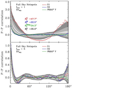
Figure 5: The P-P hotspot correlation function on the full-sky with $\ell_{\rm rmv}=1$ and 5. The green dots corresponds to the WMAP V band data, and the red and blue dots are for two simulations marked S1 and S2, respectively. For $\ell_{\rm rmv}=1$, $\theta_{0}$s give the angular scales of the correlation functions at the first zero-crossing. The correlations for $\ell_{\rm rmv}=5$ are less structured and fit the simulated statistical distribution, with few points outside $3\sigma$ confidence.

Since the correlation results, as well as our 1-point statistics, for the observed sky show sensitivity to the first 5 large angular-scale modes, it is worth analysing the large-scale phase pattern with the help of the structure of the correlation functions. The best-fitting multipoles as removed from the data are evaluated on the sky region outside the KQ75 mask. It is inevitable that the derived modes are coupled for such incomplete sky-coverage and our best-fitting amplitudes also vary with the number of modes included in the fit. However, such behaviour will also be found in the reference set of simulations, whereas other unusual properties of these modes, such as intrinsic correlations and alignments will not be. The analysis presented here will give a first assessment of the relation between the large-scale temperature distribution and the local extrema correlation structures.

We focus on the full-sky hotspots correlations, and in particular the $2\sigma_{\rm sky}$ threshold for P-P, with only the monopole and dipole removed. An identical analysis can be applied to cold spots. Two extremely behaved simulations, S1 and S2 hereafter, are selected from our samples to make a comparison with the WMAP one in Figure 5. S1 corresponds to a $\chi^{2}_{s}$-frequency 1.0000 and S2 to $\chi^{2}_{s}(30^{\circ})$-frequency 0.9970. S1 demonstrates strong spatial correlation over a range of angular serparations before declining to zero at $\theta^{S1}_{0}=47.7^{\circ}$ (within $2\sigma$ confidence). Conversely, S2 is highly suppressed on small separation scales with the zero-crossing at $\theta^{S2}_{0}=22.5^{\circ}$, and shows a similar structure to the WMAP data. The median determined from our ensemble of simulations first crosses zero at $35^{\circ}$, with the WMAP one at $24.3^{\circ}$ around the $2\sigma$ lower bound.

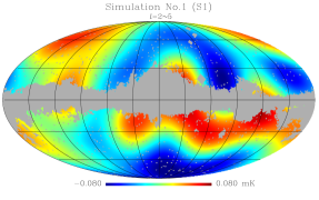
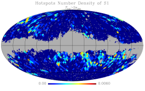
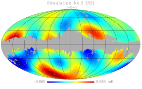
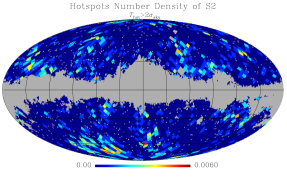
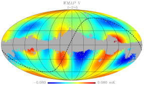
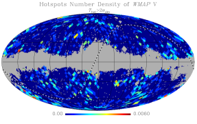
Figure 6: Left: The coadded low order moments $\ell=2\sim 5$ determined from (top to bottom) S1, S2 and the WMAP V band, shown in the Galactic coordinate system with a $30^{\circ}$ scalar graticule. Right: The corresponding number-density of hotspots for a $2\sigma_{\rm sky}$ temperature evaluated at resolution $N_{\rm side}=16$. The KQ75 mask has been applied to the maps ad shown in gray. The black dashed line on the bottom panel marks the Ecliptic plane.

We plot the coadded large-scale moments from $\ell=2$ to 5 in Figure 6, as well as the number-density of hotspots above $2\sigma_{\rm sky}$, making a comparison with the correlation structures. In particular, we note that the strong P-P correlation of S1 below $\theta_{0}$ is related to the large and continuous hot area, while the hot regions of S2 and WMAP are smaller and more scattered, which can be visually recognized from the number-density realizations and gives strong connection between the structure of extreme-hotspots and the large-scale modes of temperature distribution. Therefore, the structures of the P-P correlation function for $\ell_{\rm rmv}=1$ are sensitive to the large-scale pattern of temperature fluctuations. When modes corresponding to $\ell_{\rm rmv}=5$ are removed (Figure 5), the correlation profile of S1, S2 and the WMAP data become less structured and more consistent with the statistical distribution determined from the simulations – the points fit the median curve well with few points outside $3\sigma$ confidence.

It is also notable from Figure 6 that a pronounced north-south (both Galactic and Ecliptic) asymmetry is visible for the hot and cold regions of the integrated large angular-scale temperature distribution in the WMAP data. This asymmetry is consistent with the statistical behaviour of the temperature extrema on the sky.

4 CONCLUSIONS

In this paper, we have investigated the statistical properties of local extrema in the five-year WMAP data release, and compared with Gaussian simulations to determine whether the observed universe is consistent with such processes. The analysis is carried out on different frequency bands and five sky-coverages. Both the one-point distribution and two-point correlation of local extrema have been studied, including their dependence on large-scale CMB moments.

The hypothesis test on one-point statistics shows good consistency of the number, mean, skewness and kurtosis values with the Gaussian model used for comparison in most conditions. A few cases of rejection occur for the mean value of cold spots, somewhat consistent with the conclusion of Larson & Wandelt (2004), but these results are not significant for all bands. Larson & Wandelt (2005) also found less significant results for the mean values after applying smoothing to the data, and attributed the earlier anomalies to the noise properties of the first-year WMAP data.

Our main results are the determination of anomalously low-variance for the local extrema, and the presence of a north-south asymmetry, the latter of which has been found to be indicated in other studies of the WMAP data using different statistical estimators. We find that the data is inconsistent with simulations at the 95% C.L. for almost all frequency bands and both full-sky and the northern hemispheres of two particular coordinate systems. We also find some measurements on various scales/thresholds that are even lower than the $3\sigma$ confidence region.

Our results argue against a residual-Galactic-foreground explanation finding that the application of larger Galactic cuts, including equatorial bands out to $30^{\circ}$ Galactic latitude, yields no improvement in the consistency of data and Gaussian model predictions. However, an improvement is observed after removing the first 5 multipole moments, with the exception of the kurtosis values for cold spots in the southern Ecliptic sky, and all the statistics are well fitted after subtraction of the first 10 moments. This strongly suggests that the anomalies are related to the first 5 large-scale moments, possibly extending to $\ell=10$. Further confirmation is found via the two-point analysis.

Two kinds of two-point correlation analysis are performed to study both the temperature behavior and spatial distribution of local extrema. Limitations of the WMAP angular resolution and data processing imply that correlation features (Heavens & Sheth, 1999) on fine-scales ($10\sim 100$ arcmin) cannot be investigated here. We find that the T-T correlation functions with applied temperature thresholds are dramatically suppressed on the full-sky and northern hemispheres. The P-P correlations determined without any applied threshold trivially oscillate around zero and lie well within the confidence regions defined by simulations. However, both the T-T correlation function without threshold and the P-P function with thresholds are suppressed on small angular separations. The $\chi^{2}_{s}$ values quantify the suppression level and some $3\sigma$ detections are found. All of this anomalous behaviour is improved for $\ell_{\rm rmv}=5$ and totally disappears for $\ell_{\rm rmv}=10$.

Using two extreme simulations from our ensemble, we demonstrate a connection between the P-P correlation structures and the pattern of the corresponding fitted large-scale moments ($\ell=$ 2–5). The number-density distribution of extreme-hotspots ($T>2\sigma_{\rm sky}$) shows apparent correlation with hot regions of such large-scale moments and so does the coldspots. For the WMAP data, it is also apparent that the northern hemisphere in both the Galactic and ecliptic coordinate systems exhibit suppressed total temperature fluctuations, which directly results in an insufficient enhancement (suppression) of hot (cold) spots from moments $\ell>5$. Therefore, the low-variance of local extrema is connected to features of large-scale moments, as is the full-scale suppression of the T-T correlation with thresholds.

References

- Barreiro et al. (1997) Barreiro R.B., Sanz J.L., Martínez-González E., Cayón L., Silk J., 1997, ApJ, 478, 1
- Bennett et al. (2003) Bennett C.L., et al., 2003, ApJS, 148, 1
- Bond & Efstathiou (1987) Bond J.R., Efstathiou G., 1987, MNRAS, 226, 655
- Coles & Barrow (1987) Coles P., Barrow J.D., 1987, MNRAS, 228, 407
- Copi et al. (2008) Copi C.J., Huterer D., Schwarz D.J., Starkman G.D., 2008, arXiv:0808.3767
- Eriksen et al. (2004) Eriksen H.K, Hansen F.K., Banday A.J., Górski K.M., Lilje P.B., 2004, ApJ, 605, 14
- Eriksen et al. (2005) Eriksen H.K, Banday A.J., Górski K.M., Lilje P.B., 2005, ApJ, 622, 58
- Eriksen et al. (2007) Eriksen H.K, Banday A.J., Górski K.M., Hansen F.K., Lilje P.B., 2007, ApJ, 660, L81
- Górski et al. (2005) Górski K.M., Hivon E., Banday A.J., Wandelt B.D., Hansen F.K., Reinecke M., Bartelmann M., 2005, ApJ, 622, 759
- Gutiérrez et al. (1994) Gutiérrez C.M., Martínez-González E., Cayón L., Rebolo R., Sanz J.L, 1994, MNRAS, 271, 553
- Hamilton (1993) Hamilton A.J., 1993, ApJ, 417, 19
- Heavens & Sheth (1999) Heavens A.F., Sheth R.K., 1999, MNRAS, 310, 1062
- Heavens & Gupta (2001) Heavens A.F., Gupta S., 2001, MNRAS, 324, 960
- Hinshaw et al. (2007) Hinshaw G., et al., 2007, ApJS, 170, 288
- Hinshaw et al. (2008) Hinshaw G., et al., 2009, ApJS, 180, 225
- Kogut et al. (1995) Kogut A., Banday A. J., Bennett C. L., Hinshaw G., Lubin P. M, Smoot G. F., 1995, ApJ, 439, L29
- Kogut et al. (1996) Kogut A., Banday A. J., Bennett C. L., Górski K. M., Hinshaw G., Smoot G. F., Wright E. L., 1996, ApJ, 464, L29
- Larson & Wandelt (2004) Larson D.L., Wandelt B.D., 2004, ApJ, 613, L85
- Larson & Wandelt (2005) Larson D.L., Wandelt B.D., 2005, arXiv:astro-ph/0505046v1
- Martínez-González & Sanz (1989) Martínez-González E., Sanz J.L., 1989, MNRAS, 237, 939
- Sazhin (1985a) Sazhin M.V., 1985a, SvA, 11, L239
- Sazhin (1985b) Sazhin M.V., 1985b, MNRAS, 216, 25
- Spergel et al. (2003) Spergel D.N., et al., 2003, ApJS, 148, 175
- Tojeiro et al. (2006) Tojeiro R., Castro P.G., Heavens A.F., Gupta S., 2006, MNRAS, 365, 265
- Vittorio & Juszkiewicz (1987) Vittorio N., Juszkiewicz R., 1987, ApJ, 314, L29
- Wandelt, Hivon & Górski (1998) Wandelt B.D., Hivon E., Górski K.M., 1998, arXiv:astro-ph/9803317v2, in Fundamental Parameters in Cosmology, Proc. 33rd Rencontres de Moriond, ed. J. Tran Thanh Van, 237
- Zabotin & Naselski (1985) Zabotin N.A., Naselski P.D., 1985, SvA, 29, 614