Entanglement and area law with a fractal boundary in a topologically ordered phase

Abstract

Quantum systems with short range interactions are known to respect an area law for the entanglement entropy: the von Neumann entropy $S$ associated to a bipartition scales with the boundary $p$ between the two parts. Here we study the case in which the boundary is a fractal. We consider the topologically ordered phase of the toric code with a magnetic field. When the field vanishes it is possible to analytically compute the entanglement entropy for both regular and fractal bipartitions $(A,B)$ of the system, and this yields an upper bound for the entire topological phase. When the $A$-$B$ boundary is regular we have $S/p=1$ for large $p$. When the boundary is a fractal of Hausdorff dimension $D$, we show that the entanglement between the two parts scales as $S/p=\gamma\leq 1/D$, and $\gamma$ depends on the fractal considered.

Introduction.— Entanglement is certainly one of the most striking aspects of quantum theory. Not only is it the key ingredient for protocols ranging from quantum teleportation to cryptography, but it also has an important role in the study of condensed matter and many body systems ent-review . Quantum phase transitions can be understood in terms of entanglement entqpt , and new exotic states of matter that defy a description in terms of local order parameters show a signature of topological order in the global pattern of their entanglement hiz ; topentropy . Moreover, the analysis of the scaling of entanglement in the ground state of condensed matter systems has shed new light on the question of their simulability vidal .

Especially for the last reason, one is interested in knowing how entanglement scales with the size of the system. If there is a gap, all correlations decay exponentially with the distance in units of the length scale hastings-gap . In this case, one also expects the entanglement to be short ranged, so that only the degrees of freedom of the boundary of the system contribute to the total entanglement. This is the so called area law for the entanglement (see Ref. arealawrev for a comprehensive review).

In this work, we study the case of a topologically ordered state, the ground state of the toric code kitaev . For this state – and a class of topologically ordered states – the entanglement can be computed exactly hiz . For a bipartition with a regular boundary $p$, the entanglement measured by the von Neumann entropy $S$ is exactly $S=p-1$, where the correction $-1$ is due to a topological contribution to the entanglement hiz ; topentropy . Obviously, $\gamma:=S/p$ is $1$ in the limit of large $p$. If we add perturbations to the model, topological order is not destroyed until a quantum phase transition happens. Throughout the entire topological phase the entanglement is upper-bounded by its value in the unperturbed model topqpt-num .

Here we study the case in which the boundary of the system is a fractal curve of Hausdorff dimension $D$. This situation arises under a large variety of experimental conditions in two-dimensional systems lidarfractal . The scaling of entanglement for self similar systems is important also in view of devising efficient algorithms which use the renormalization group for computing ground states of quantum systems in two dimensions vidal . One could expect that as the boundary of the system becomes less regular, the entanglement increases with the length $p$ of the boundary, as in the case of fermions fermions . In contrast to the fermionic case, we find that for topologically ordered spin systems the entanglement decreases with $p$. The length of a fractal curve – and consequently the entanglement – diverges in the limit of exact fractality fractalbook . However, for every step $n$ of the iteration of the fractal, the length of the curve is a finite number $p(n)$, which increases with $n$. In contrast to regular boundaries, for fractal boundaries $\gamma$ is a fractional number: we can speak of fractal entanglement. Moreover, we shall see that $\gamma\leq D^{-1}$.

Entanglement and topological order.— Consider a unitary representation of a group $G$ acting on spin-$1/2$ degrees of freedom with Hilbert space ${\cal H}$. Since we wish to compute the entanglement entropy associated to a bipartition of the system, we are interested in the properties of the group when we split the Hilbert space as ${\cal H}={\cal H}_{A}\otimes{\cal H}_{B}$. We assume that there exists a product state $|0\rangle=|0_{A}\rangle\otimes|0_{B}\rangle\in{\cal H}$. We can now define the (normalized) $G$-state as $|\Psi_{G}\rangle:=\sum_{g\in G}\alpha(g)g|0\rangle$. If all the coefficients are equal, we call the state a $G$-uniform state: $|G\rangle:=|G|^{-1/2}\sum_{g\in G}g|0\rangle$, where $|G|$ is the order of $G$. Note that $|G\rangle$ is stabilized by the group $G$. Let us now define the two subgroups of $G$ that act trivially on the subsystems $A,B$ respectively: $G_{A}:=\{g\in G\ |\ \ g=g_{A}\otimes{\mathchoice{\rm 1\mskip-4.0mul}{\rm 1\mskip-4.0mul}{\rm 1\mskip-4.5mul}{\rm 1\mskip-5.0mul}}_{B}\}$ and similarly for $G_{B}$. By defining the quotient group $G_{AB}:=G/(G_{A}\times G_{B})$, we can write $G$ as the union over all elements of $G_{AB}$: $G=\bigcup_{[h]\in G_{AB}}\{(g_{A}\otimes g_{B})h\,|\ g_{A}\otimes{\mathchoice{\rm 1\mskip-4.0mul}{\rm 1\mskip-4.0mul}{\rm 1\mskip-4.5mul}{\rm 1\mskip-5.0mul}}_{B}\in G_{A},\,{\mathchoice{\rm 1\mskip-4.0mul}{\rm 1\mskip-4.0mul}{\rm 1\mskip-4.5mul}{\rm 1\mskip-5.0mul}}_{A}\otimes g_{B}\in G_{B}\}$. The state can thus be written as $|\Psi_{G}\rangle=|G|^{-1/2}\sum_{\begin{subarray}{c}g_{A}\otimes g_{B}\in G_{A}\times G_{B}\\ h\in G_{AB}\end{subarray}}\alpha(g_{A}\otimes g_{B},h)h_{A}\otimes h_{B}\otimes(g_{A}\otimes g_{B})|0\rangle$. If the coefficients $\alpha$ in the expression for $|\Psi_{G}\rangle$ satisfy the separability condition $\alpha(g_{A}\otimes g_{B},h)\equiv\alpha(g_{A}\otimes g_{B}h_{g})=\alpha_{A}(g_{A})\alpha_{B}(g_{B})\beta(h_{g})$ for every $g\in G$, then it is possible to prove hiz2 that the von Neumann entropy of the $G$-state corresponding to the bipartition $(A,B)$ is: $S(|\Psi_{G}\rangle)=-\sum_{[h]\in G_{AB}}|N_{A}N_{B}\beta(h)|^{2}\log_{2}|N_{A}N_{B}\beta(h)|^{2}$, where $N_{X}^{2}:=\sum_{g_{X}\in G_{X}}|\alpha_{X}(g_{X})|^{2}$, for $X=A,B$. By convexity of $S$ we have $S(|\Psi_{G}\rangle)\leq S(|G\rangle)=\log_{2}|G_{AB}|$.

This formalism is remarkably well suited to describing topologically ordered states. In many quantum spin systems, topological order arises from a mechanism of closed string condensation and the group $G$ is the group of closed strings on a lattice closedstrings . An important example of topologically ordered system is given by Kitaev’s toric code, which provides a model for which at zero temperature topological memory and topological quantum computation are robust against arbitrary local perturbations kitaev . The model is defined on a square lattice with spin-$1/2$ degrees of freedom on the edges and periodic boundary conditions. To every plaquette $p$ we associate the operator product of $\sigma^{x}$ on all the spins that comprise the boundary of $p$, i.e., $X_{p}=\prod_{j\in p}\sigma^{z}_{j}$. To every vertex $s$ we associate the product of $\sigma^{z}$ on all the spins connected to $s$: $Z_{s}=\prod_{j\in s}\sigma^{x}_{j}$. The operators $X_{p}$ generate a group $G$ of closed string-nets. The Hamiltonian of the toric code in an external magnetic field is:

$$H_{\rm toric}=-\sum_{p}X_{p}-\lambda\sum_{s}Z_{s}+(1-\lambda)\sum_{j}\sigma^{z}_{j},$$ (1)

where we have introduced a control parameter $\lambda$. A second order quantum phase transition at $\lambda_{c}\sim 0.7$ separates a spin-polarized phase ($0\leq\lambda<\lambda_{c}$) from a topologically ordered phase ($\lambda_{c}<\lambda\leq 1$) top-qpt ; topqpt-num . The ground state of $H_{\rm toric}$ is a $G$-state throughout the entire topological phase. It is $G$-uniform at the toric code point $\lambda=1$, and becomes less uniform as $\lambda$ decreases to $\lambda_{c}$.

We now wish to argue that the separability condition for $\alpha(g)$ is satisfied throughout the entire topological phase, and hence by convexity $S_{\lambda}\leq S(|G\rangle)=\log_{2}|G_{AB}|$ for $\lambda_{c}<\lambda\leq 1$, with the bound saturated at the toric code point. At $\lambda=0$ the ground state is the uniform superposition of closed strings. The $\lambda$ term in Eq. (1) is a tension for the strings. As we increase $\lambda$, larger strings become less favored in the ground state. Everywhere in the topological phase, that is, for sufficiently small $\lambda$, the ground state is still the superposition (with positive coefficients topqpt-num ) of closed strings $g\in G$. The expectation value $\langle g\rangle$ of any closed string $g\in G$ of length $l$ (a Wilson loop) can be written as $\langle g\rangle=C_{t}^{2}e^{(1-\lambda)l(g)}$, where $C_{t}$ is a constant that does not depend on $g$ (due to translational invariance). Similarly, in the polarized phase we have $\langle g\rangle=C_{p}^{2}e^{-\lambda a(g)}$, where $a$ is the area enclosed by the string Kogut . Now, we know that $\langle g\rangle=|\alpha(g)|^{2}$ at any point in the topological phase, since the ground state is a $G$-state and does not contain any open strings. Since the length $l$ for a given string $g=g_{A}\otimes g_{B}h_{g}$ can be decomposed as a sum of the corresponding substrings, $l=l_{A}+l_{B}+l_{AB}$, we have $\alpha(g)=C_{t}e^{-l(g)/2}=C_{t}e^{-l_{A}/2}e^{-l_{B}/2}e^{-l_{AB}/2}\equiv\alpha_{A}(g_{A})\alpha_{B}(g_{B})\beta(h_{g})$, i.e., we have separability.

Fractal boundary.— Henceforth we consider the toric code point $\lambda=1$, where $S=\log_{2}|G_{AB}|$. We define bipartitions by drawing strings along the edges of the lattice. One can prove hiz that $\log_{2}|G_{AB}|$ is the number of independent plaquette operators $A_{p}$ acting on both subsystems $A$ and $B$, which in turn is the number of squares that have at least one side adjacent to the boundary $p$ of the region $\mathcal{A}$, see Fig. 1. How do we measure $p$? We shall show that the support of the mixed part of the reduced density matrix is given exclusively by the spins on the boundary. This mixed part is the only part contributing to the entanglement between the $A$ and $B$ partitions. Therefore we define the length $p$ as the number of boundary spins. Indeed, letting $Q_{X}=|G_{X}|^{-1/2}\sum_{g_{X}\in G_{X}}g_{X}$, with $X=A,B$, the ground state can be written as $|G\rangle=|G_{AB}|^{-1/2}\sum_{h\in G_{AB}}h_{A}h_{B}Q_{A}Q_{B}|0\rangle$. It follows from the definition of $G_{AB}$ that we can pick $h_{A}$ up to local transformations of the loops inside $A$ and $B$. Specifically, we can pick $h_{A}$ as acting only on the spins on the boundary. Since $Q_{A},Q_{B}$ are local operators, the reduced density matrix of the $A$-subsystem is equivalent to one separable as ${\mbox{Tr\,}}_{B}[|G\rangle\langle G|]=|\psi\rangle\langle\psi|\otimes\tilde{\rho}_{A}$, where $|\psi\rangle$ is a pure state describing $A$’s bulk, while the mixed part is $\tilde{\rho}_{A}=|G_{AB}|^{-1}\sum_{h\in G_{AB}}h_{A}|0\rangle\langle 0|h_{A}$, where $h_{A}$ acts exclusively on the spins along the boundary of $A$ fhhw . Thus $S/p$ is the average entanglement per spin in the support of $\tilde{\rho}_{A}$.

We now consider the case of a bipartition defined by a closed fractal curve. Since the model studied here is defined on a square lattice, we consider bounded regions of $\mathbb{Z}^{2}$ depending on a parameter $n$, denoted by $\mathcal{A}_{n}$. Here $n$ represents the number of steps in the iteration generating the fractal curve. The perimeter of $\mathcal{A}_{n}$ is denoted by $p\left(\mathcal{A}_{n}\right)$. The number of squares of size one adjacent to the boundary of $\mathcal{A}_{n}$ is the entanglement $S(\mathcal{A}_{n})$ associated to the bipartition $(\mathcal{A}_{n},\mathcal{B}_{n})$. We are interested in the large $n$ limit of the ratio between entanglement and perimeter: $\gamma\left(\mathcal{A}\right):=\lim_{n\rightarrow\infty}S(\mathcal{A}_{n})/p(\mathcal{A}_{n})$. One might expect the scaling law $S=p-1$ to be independent of the geometric properties of the bipartition, but this is not the case. From Fig. 1, we see that when the boundary of $A$ has some inward angles, or wells, or other “kinks”, the number of squares adjacent to it is less than the length of the boundary around it. For instance, an inward angle, a well, and a hole all have just one adjacent square of side $1$ but they have lengths $2,3,4$ in the lattice spacing unit, respectively. We call $\alpha$ and $h$ the number of inward angles and holes, respectively. It is not hard to show that comment

$$S=p-\alpha-3h.$$ (2)

We wish to study how these numbers scale for a fractal expansion, and find the corresponding scaling of the entanglement.

In the following, we shall compute $\gamma$ for several fractal curves. The results are summarized in Table 1. The main result is that, depending on the fractal region, $\gamma$ can be a fractional number. The Hausdorff dimension $D$ of the fractal does not uniquely determine the value of $\gamma$, but (in all the examples considered) we have the bound $\gamma\leq D^{-1}$.

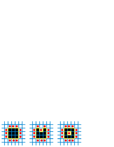
Figure 1: The drawings show different bipartitions of the system. The subsystem $\mathcal{A}$ consists of all the spins marked by the black squares. The entanglement is given by the number of plaquette operators acting on both subsystems, marked by red dots. For a regular figure (left), this number coincides with the perimeter $p$, which is the number of spins along the boundary (in yellow). Every time there is an inward angle, there is one such operator for three units of length. The well (middle) contains two inward angles. A hole (right) of size $1$ accounts for $4$ units of length and contains only one star operator.

Examples.— The Sierpinski carpet on $\mathbb{Z}^{2}$, denoted by $\mathcal{S}_{n}$, is a bounded region of $\mathbb{Z}^{2}$ defined iteratively in the following way: (i) $\mathcal{S}_{1}$ is a $3\times 3$ square without the central $1\times 1$ square. The Sierpinski carpet $\mathcal{S}_{1}$ has a single square hole. (ii) $\mathcal{S}_{n+1}$ is a bounded region inscribed on a $3^{n}\times 3^{n}$ square on $\mathbb{Z}^{2}$. This is obtained by placing $8$ copies of $\mathcal{S}_{n}$ on all quadrants of the square, but the central one (see Fig. 2). Given the recursive structure of $\mathcal{S}_{n}$, direct calculations show that $\alpha(\mathcal{S}_{n})=\frac{1}{14}8^{n}-\frac{4}{7}$. The number of equal holes of side $3^{i}$ is $8^{n-1-i}$, so $h(n)=8^{n-1}$. Observe that the external perimeter of $\mathcal{S}_{n}$ is $4\times 3^{n}$. Then the perimeter $p(n)$ is $p(\mathcal{S}_{n})=4(3^{n}+3^{n-1}+\sum\nolimits_{i=0}^{n-2}(3^{i}\times 8^{n-1-i}))=4\left(4\times 3^{n}+8^{n}\right)/5$. With this information, from Eq. (2) we obtain $\gamma\left(\mathcal{S}_{n}\right)=99/224$.

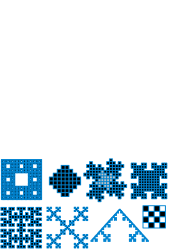
Figure 2: (Color online) Top, left to right: Sierpinski carpet $\mathcal{S}_{3}$, Greek cross $\mathcal{G}_{3}$, Minkowski sausage $\mathcal{I}_{3}$, T-square $\mathcal{E}_{4}$. Bottom, left to right: Moore polygons $\mathcal{M}_{3}$, Vicsek fractal $\mathcal{V}_{3}$, half perimeter of the Koch polygon $\mathcal{K}_{5}$, $4\times 4$ chessboard $\mathcal{C}_{4}$.

The Greek cross on $\mathbb{Z}^{2}$, denoted by $\mathcal{G}_{n}$, is a polygon in $\mathbb{Z}^{2}$ defined by a closed path of length $p\left(\mathcal{G}_{n}\right)=8n+8$, including the point $\left(0,n\right)$ and the step $\left\{(0,n),(1,n)\right\}$. The path maximizes the number of inward angles over all the closed paths of the same length including the point $\left(0,n\right)$. Fig. 2 gives the first few instances. It is then evident that $\alpha(\mathcal{G}_{n})=4n$. For this polygon, $h(n)=0$ and thus from Eq. (2) we have $S(n)=p(n)-\alpha(n)$. Therefore, $\gamma\left(\mathcal{G}_{n}\right)=1/2$.

The Minkowski sausage $\mathcal{I}_{n}$ is a polygon in $\mathbb{Z}^{2}$ defined as follows: (i) $\mathcal{I}_{0}$ is a square of side one. (ii) $\mathcal{I}_{n+1}$ is obtained by replacing each side of $\mathcal{I}_{n}$ by a path of length three. The angles in the path are determined by the position of the side in $\mathcal{I}_{n}$. The first and third segments of the path follow the direction of the replaced side. The two angles are first left then right. Analogously, we can construct $\mathcal{I}_{n+1}$ by attaching to the sides of $\mathcal{I}_{n}$ four of its copies (see Fig. 2). The polygon $\mathcal{I}_{n}$ can be used to tessellate the plane. From the definition, we can determine $p\left(\mathcal{I}_{n}\right)=4\times 3^{n}$ and $\alpha\left(\mathcal{I}_{n}\right)=2\times 3^{n}-2$. Here too we have $S(n)=p(n)-\alpha(n)$. Hence, $\gamma\left(\mathcal{I}_{n}\right)=1/2$.

The Moore polygon $\mathcal{M}_{n}$ is a “closed version” of the Moore curve. It is a polygon in $\mathbb{Z}^{2}$ defined by a closed path expressed as an $L$-system. A Lindenmayer system (for short, $L$-system) rs80 is a quadruple $\left\langle V,C,A,R\right\rangle$, where $V$ is a set of variables, $C$ a set of constants, $A$ a set of axioms, and $R$ a set of production rules. An $L$-system allows the recursive construction of words (or, equivalently, sequence of symbols) whose letters are elements from $V$ and $C$. An axiom is a word at time $t=0$. At each time step $t+1$, the production rules are applied to the word given by the $L$-system at time $t$. Only variables are replaced according to the production rules. On the basis of these definitions, we can write $\mathcal{M}_{n}=\left\langle V,C,A,R\right\rangle$, where $V=\{a,b\}$, $C=\{+,-\}$, $A=\{aFa+F+aFa\}$, and $R=\{a\rightarrow-bF+aFa+Fb-,b\rightarrow+aF-bFb-Fa+\}$. The letter $F$ indicates a segment of length one in $\mathbb{Z}^{2}$. The first segment of $\mathcal{M}_{0}$ specified by the axiom in $A$ is $\{(0,0),(1,0)\}$. The symbols $+$ and $-$ mean “turn left in $\mathbb{Z}^{2}$” and “turn right in $\mathbb{Z}^{2}$”, respectively. The sequences $-+$ and $+-$ have no meaning and can be deleted. For instance, the polygon $\mathcal{M}_{1}$ is then given by the the following word: $-bF+aFa+Fb-F-bF+aFa+FbFbF+aFa+Fb-F-bF+aFa+Fb-F$. Notice that in order to close $\mathcal{M}_{1}$ we need to replace $\cdots+Fb-F$ with $\cdots+FbF$ in the obtained word. This operation is required for every $n$. Once we have generated the polygon, we blow it up by replacing each square of side one with a square comprising four of its copies. The occurrences of letter $F$ in the word produced by $\mathcal{M}_{1}$ is $16$. In general, the number of occurrences of $F$ in the word produced by $\mathcal{M}_{n}$ equals the perimeter of $\mathcal{M}_{n}$. From the definition, this is $p(\mathcal{M}_{n})=2\times 4^{n+1}$, taking into account the blowing up operation. The number of $-$ (“turn right”) symbols, excluding the initial one, in the word produced by $\mathcal{M}_{n}$, is exactly equal to the number of inward angles of $\mathcal{M}_{n}$: $\alpha(\mathcal{M}_{n})=\frac{2}{5}\left(-1\right)^{n}+\frac{8}{5}4^{n}-2$. From $S=p(\mathcal{M}_{n})-\alpha(\mathcal{M}_{n})$, we can compute $\gamma\left(\mathcal{M}_{n}\right)=4/5$.

The Vicsek snowflake on $\mathbb{Z}^{2}$, denoted by $\mathcal{V}_{n}$, is a bounded region of $\mathbb{Z}^{2}$ defined iteratively as follows: (i) $\mathcal{V}_{0}$ is a single $1\times 1$ square. (ii) We obtain $\mathcal{V}_{n+1}$ by attaching $4$ copies of $\mathcal{V}_{n}$ to its corners (see Fig. 2). Each square comprising $\mathcal{V}_{n}$ has side one. For this fractal we have $p\left(\mathcal{V}_{n}\right)=20\times 5^{n-1}$ and $\alpha\left(\mathcal{V}_{n}\right)=2\times 5^{n}-2$. The number of adjacent squares is $S(n)=p(n)-\alpha(n)$, which gives $\gamma(\mathcal{V})=\frac{1}{2}$.

The quadratic Koch polygon, $\mathcal{K}_{n}$, is a polygon in $\mathbb{Z}^{2}$ based on the Koch curve. Essentially, it consists of a region bounded by two mirroring copies of the Koch curve. As the Moore polygon, $\mathcal{K}_{n}$ is defined by an $L$-system and specified by a path. The path giving rise to $\mathcal{K}_{0}$ is given axiomatically as $\{(0,0),(1,0)\}$. Then $\mathcal{K}_{0}$ is a square of side one. The production rule is $F\rightarrow F+F-F-F+F$, where $F$ indicates again a segment of length one in $\mathbb{Z}^{2}$. The fractal has a pattern similar to that of the Vicsek snowflake and indeed has the same Hausdorff dimension (see Table 1). Nevertheless, the results for the scaling of the entanglement are different. The perimeter can be computed as $p(n)=4\times 5^{n}$. The number $h(n)$ of holes is $h=\frac{18}{125}\times 5^{n}+\frac{1}{3}3^{n}-1$, for $n\geq 3$. One can easily see that $\alpha=(p-4h)/2$ and therefore from Eq. (2) $S=\frac{p}{2}-h=\frac{232}{125}5^{n}-\frac{1}{3}3^{n}+1$. In the limit of large $n$, we obtain $\gamma=58/125$.

The T-square polygon on $\mathbb{Z}^{2}$, $\mathcal{E}_{n}$, is obtained by superimposing four copies of $\mathcal{E}_{n-1}$ on the corners of a square of side $2^{n+1}$. The area covered by each copy is exactly a square of side $2^{n}$. The perimeter of $\mathcal{E}_{n}$ is $p\left(\mathcal{E}_{n}\right)=16\times 3^{n}-8\times 2^{n}$. We have $S\left(\mathcal{E}_{0}\right)=4$, $S\left(\mathcal{E}_{1}\right)=24$, and $S\left(\mathcal{E}_{n}\right)=3S\left(\mathcal{E}_{n-1}\right)+2^{n+1}-8=\frac{80}{9}3^{n}+2^{n+1}-8+24\times S(n,3)=\frac{92}{9}3^{n}-4\times 2^{n}+4,$ where $\mathcal{S}(n,3):=(1+3^{n-2}-2^{n-1})/2$ is the $n$-th Stirling number of the second kind. Hence, $\gamma=1/2$.

The chessboard $\mathcal{C}_{n}$ is the bounded region of $\mathbb{Z}^{2}$ defined as follows. Let $\mathcal{C}_{1}$ be a $2\times 2$ square with two holes in the upper right and bottom left corner. Then $\mathcal{C}_{n+1}$ is obtained by placing $4$ copies of $\mathcal{C}_{n}$ on all the quadrants of a $2^{n}\times 2^{n}$ square on $\mathbb{Z}^{2}$. The perimeter is $p=2n$. The number of adjacent squares is exactly $h=n/2$. Therefore it is immediate that $\gamma=N_{s}/p=1/4$ for every size $n$. It is obvious that this is a lower bound for the entanglement on the square lattice for a state in $\mathcal{L}$, since the chessboard maximizes the number of holes of side $1$.

Table 1: Fractal entanglement $\gamma$, perimeter $p(n)$, entropy of entanglement $S(n)$ for a state in $\mathcal{L}$ for several fractal bipartitions $(A,B)$ of the square lattice. Here $D$ is the Hausdorff dimension of the curve separating the regions ${\mathcal{A}}_{n}$ and ${\mathcal{B}}_{n}$. For $p(n)$ and $S(n)$ only the leading term is shown.

Fractal	$\gamma$	$p(n)$	$S(n)$	$D$
1. Sierpinski carpet	$\frac{99}{224}$	$\frac{4}{5}8^{n}$	$\frac{99}{280}8^{n}$	$\frac{\log 8}{\log 3}$
2. Greek Cross	$\frac{1}{2}$	$8n$	$4n$	$2$
3. Minkowski Sausage	$\frac{1}{2}$	$4\times 3^{n}$	$2\times 3^{n}$	$\frac{\log 5}{\log 3}$
4. Vicsek Snowflake	$\frac{1}{2}$	$4\times 5^{n}$	$2\times 5^{n}$	$\frac{\log 5}{\log 3}$
5. Quadratic Koch	$\frac{58}{125}$	$4\times 5^{n}$	$\frac{232}{125}5^{n}$	$\frac{\log 5}{\log 3}$
6. Moore Polygon	$\frac{4}{5}$	$2\times 4^{n+1}$	$\frac{32}{5}4^{n}$	$\frac{\log 9}{\log 6}$
7. T-Square	$\frac{1}{2}$	$16\times 3^{n}$	$\frac{92}{9}3^{n}$	$2$
8. Chessboard	$\frac{1}{4}$	$8n^{2}$	$2n^{2}$	$2$

Conclusions.—This work has, for the first time, explored the relationship between entanglement entropy and the fractality of the bipartition in a spin system. We have calculated the scaling of entanglement $S$ with the length $p$ of the boundary in the ground state of the $Z_{2}$ topological phase associated with the toric code, for various fractal boundaries. We have shown that this provides an upper bound on the entanglement in the entire topological phase. Unlike the case of a regular boundary, the ratio $\gamma=S/p$ for large $p$ is not exactly $1$ but a smaller fraction, so that the general bound for the area law is still obeyed. The fractal nature of the bipartition is revealed in the total amount of entanglement present in the system. There is less entanglement in a fractal bipartition. We also found that the ratio $\gamma$ is always at most the inverse of the Hausdorff dimension $D$. We conjecture this last claim to hold in general for topologically ordered states. Moreover, different fractals with the same Hausdorff dimension can have different $\gamma$, so that this is a useful quantity to classify fractals with. We chose the toric code because in this case it is simple to compute the entanglement. It would be interesting to consider other types of topologically ordered states and explore whether the behavior we have observed is general for any quantum system with finite correlation length. Finally, since the scaling of entanglement with the boundary of the system is less than $1$, we believe that a renormalization group algorithm based on blocks of spins that grow like fractals, might be potentially more efficient. Indeed, in this regard the chessboard appears to be the most attractive of all the fractals we have considered.

Acknowledgments.—Research at Perimeter Institute for Theoretical Physics is supported in part by the Government of Canada through NSERC and by the Province of Ontario through MRI. D.A.L.’s work was supported by NSF under grants No. CCF-726439, No. PHY-802678 and No. PHY-803304. D.A.L. acknowledges the hospitality of IQI-Caltech where part of this work was performed. Research at IQC is supported by DTOARO, ORDCF, CFI, CIFAR, and MITACS.

References

- (1) L. Amico, R. Fazio, A. Osterloh, and V. Vedral, Rev. Mod. Phys. 80, 517 (2008).
- (2) A. Osterloh, L. Amico, G. Falci, R. Fazio, Nature 416, 608 (2002); T.J. Osborne and M.A. Nielsen, Phys. Rev. A 66, 032110 (2002); G. Vidal, J.I. Latorre, E. Rico, A. Kitaev, Phys. Rev. Lett. 90, 227902 (2003); F. Verstraete, M. Popp, J. I. Cirac, Phys. Rev. Lett. 92, 027901 (2004); L.-A. Wu, M.S. Sarandy, D.A. Lidar, Phys. Rev. Lett. 93, 250404 (2004).
- (3) A. Hamma, R. Ionicioiu, P. Zanardi, Phys. Lett. A 337, 22 (2005); ibid., Phys. Rev. A 71, 022315 (2005)
- (4) A. Kitaev, J. Preskill, Phys. Rev. Lett. 96, 110404 (2006); M. Levin, X.-G. Wen, Phys. Rev. Lett. 96, 110405 (2006).
- (5) G. Vidal, Phys. Rev. Lett. 99, 220405 (2007).
- (6) M.B. Hastings, T. Koma, Comm. Math. Phys. 265, 781 (2006).
- (7) J. Eisert, M. Cramer, M.B. Plenio, eprint arXiv:0808.3773.
- (8) M.M. Wolf, F. Verstraete, M.B. Hastings, J.I. Cirac, Phys. Rev. Lett. 100, 070502 (2008).
- (9) A.Y. Kitaev, Annals of Phys. 303, 2 (2003).
- (10) A. Hamma, W. Zhang, S. Haas, D. Lidar, Phys. Rev. B 77, 155111 (2008).
- (11) B. Kogut, Rev. Mod. Phys. 51, 659 (1979).
- (12) O. Malcai, D.A. Lidar, O, Biham, D. Avnir, Phys. Rev. E 56, 2817 (1997).
- (13) M. Barnsley, Fractals everywhere (Academic Press, New York, 1988).
- (14) X.-G. Wen, Quantum Field Theory of Many-Body Systems, (Oxford Univ. Press, Oxford, 2004).
- (15) A. Hamma, D.A. Lidar, Phys. Rev. Lett. 100, 030502 (2008); S. Trebst et al., Phys. Rev. Lett. 98, 070602 (2007).
- (16) A. Hamma, R. Ionicioiu, P. Zanardi, Phys. Rev. A 72, 012324 (2005).
- (17) S.T. Flammia, A. Hamma, T.L. Hughes, X.-G. Wen, Phys. Rev. Lett. 103, 261601 (2009).
- (18) The entanglement is the number of squares in the dual lattice that have at least one side adjacent to the boundary of the region . For a figure that is a square of perimeter with a hole in the bulk, the total perimeter is . The number of adjacent squares is because there are adjacent squares on the external boundary, and one inside. Thus . With holes we have and , so that . A similar counting argument which accounts for inward angles leads to Eq. (2).
- (19) D. Gioev, and I. Klich, Phys. Rev. Lett. 96, 100503 (2006).
- (20) G. Rozenberg and A. Salomaa, The mathematical theory of L systems (Academic Press, New York, 1980).