Recent Advances in Chromospheric and Coronal Polarization Diagnostics

Abstract

I review some recent advances in methods to diagnose polarized radiation with which we may hope to explore the magnetism of the solar chromosphere and corona. These methods are based on the remarkable signatures that the radiatively induced quantum coherences produce in the emergent spectral line polarization and on the joint action of the Hanle and Zeeman effects. Some applications to spicules, prominences, active region filaments, emerging flux regions and the quiet chromosphere are discussed.

1 Introduction

The fact that the anisotropic illumination of the atoms in the chromosphere and corona induces population imbalances and quantum coherences between the magnetic sublevels, even among those pertaning to different levels, is often considered as a hurdle for the development of practical diagnostic tools of “measuring” the magnetic field in such outer regions of the solar atmosphere. However, as we shall see throughout this paper, it is precisely this fact that gives us the hope of reaching such an important scientific goal. The price to be paid is that we need to develop high-sensitivity spectropolarimeters for ground-based and space telescopes and to interpret the observations within the framework of the quantum theory of spectral line formation. As J.W. Harvey put it, “this is a hard research area that is not for the timid” (Harvey (2006)).

Rather than attempting to survey all of the literature on the subject, I have opted for beginning with a very brief introduction to the physics of spectral line polarization, pointing out the advantages and disadvantages of the Hanle and Zeeman effects as diagnostic tools, and continuing with a more detailed discussion of selected developments. Recent reviews where the reader finds complementary information are Harvey (2006), Stenflo (2006), Lagg (2007), López Ariste & Aulanier (2007), Casini & Landi Degl’Innocenti (2007), and Trujillo Bueno (2009).

2 The physical origin of the spectral line polarization

Solar magnetic fields leave their fingerprints in the polarization signatures of the emergent spectral line radiation. This occurs through a variety of rather unfamiliar physical mechanisms, not only via the Zeeman effect. In particular, in stellar atmospheres there is a more fundamental mechanism producing polarization in spectral lines. There, where the emitted radiation can escape through the stellar surface, the atoms are illuminated by an anisotropic radiation field. The ensuing radiation pumping produces population imbalances among the magnetic substates of the energy levels (that is, atomic level polarization), in such a way that the populations of substates with different values of $|M|$ are different ($M$ being the magnetic quantum number). This is termed atomic level alignment. As a result, the emission process can generate linear polarization in spectral lines without the need for a magnetic field. This is known as scattering line polarization (e.g., Stenflo (1994), Landi Degl’Innocenti & Landolfi (2004)). Moreover, radiation is also selectively absorbed when the lower level of the transition is polarized (Trujillo Bueno & Landi Degl’Innocenti (1997), Trujillo Bueno (1999), Trujillo Bueno et al. (2002b), Manso Sainz & Trujillo Bueno (2003b)). Thus, the medium becomes dichroic simply because the light itself has the chance of escaping from it.

Upper-level polarization produces selective emission of polarization components, while lower-level polarization produces selective absorption of polarization components. A useful expression to estimate the amplitude of the emergent fractional linear polarization is the following generalization of the Eddington-Barbier formula (Trujillo Bueno (2003a)), which establishes that the emergent $Q/I$ at the center of a sufficiently strong spectral line when observing along a line of sight (LOS) specified by $\mu=\cos\theta$ (with $\theta$ being the angle between the local solar vertical and the LOS) is approximately given by

$${{Q}\over{I}}\,{\approx}\,{3\over{2\sqrt{2}}}(1-\mu^{2})\,[{\cal W}\,\sigma^{2}_{0}({J_{u}})\,-\,{\cal Z}\,\sigma^{2}_{0}({J_{l}})]\,=\,{3\over{2\sqrt{2}}}(1-\mu^{2})\,\,{\cal F},$$ (1)

where ${\cal W}$ and ${\cal Z}$ are numerical factors that depend on the angular momentum values ($J$) of the lower ($l$) and upper ($u$) levels of the transition (e.g., ${\cal W}={\cal Z}=-1/2$ for a line with $J_{l}=J_{u}=1$), while $\sigma^{2}_{0}=\rho^{2}_{0}/\rho^{0}_{0}$ quantifies the fractional atomic alignment of the upper or lower level of the spectral line under consideration, calculated in a reference system whose $Z$-axis (i.e., the quantization axis of total angular momentum) is along the local solar vertical. The $\sigma^{2}_{0}(J)$ values quantify the degree of population imbalances among the sublevels of level $J$ with different $|M|$-values. They have to be calculated by solving the statistical equilibrium equations for the multipolar components of the atomic density matrix (see Chapt. 7 of Landi Degl’Innocenti & Landolfi (2004)). In a weakly anisotropic medium like the solar atmosphere, the $\sigma^{2}_{0}(J_{l})$ and $\sigma^{2}_{0}(J_{u})$ values of a resonance line transition are proportional to the so-called anisotropy factor $w=\sqrt{2}J^{2}_{0}/J^{0}_{0}$ (e.g., §3 in Trujillo Bueno (2001)), where $J^{0}_{0}$ is the familiar mean intensity and ${J}^{2}_{0}\approx\oint{\rm d}\vec{\Omega}/(4\pi)\,1/(2\sqrt{2})\,(3\mu^{2}-1)\,{{I_{\nu,\vec{\Omega}}}}\,$ quantifies whether the illumination of the atomic system is preferentially vertical ($w>0$) or horizontal ($w<0$). Note that in Eq. (1) the $\sigma^{2}_{0}$ values are those corresponding to the atmospheric height where the line-center optical depth is unity along the LOS.

The most practical aspect is that a magnetic field inclined with respect to the symmetry axis of the pumping radiation field modifies the atomic level polarization via the Hanle effect (e.g., the reviews by Trujillo Bueno (2001), Trujillo Bueno (2005); see also Landi Degl’Innocenti & Landolfi (2004)). Approximately, the amplitude of the emergent spectral line polarization is sensitive to magnetic strengths between $0.1\,B_{\rm H}$ and $10\,B_{\rm H}$, where the critical Hanle field intensity ($B_{\rm H}$, in gauss) is that for which the Zeeman splitting of the $J$-level under consideration is equal to its natural width:

$$B_{\rm H}=1.137{\times}10^{-7}/(t_{\rm life}\,g_{J})$$ (2)

with $t_{\rm life}$ the lifetime, in seconds, of the $J$-level under consideration and $g_{J}$ its Landé factor. Since the lifetimes of the upper levels ($J_{u}$) of the transitions of interest are usually much smaller than those of the lower levels ($J_{l}$), clearly diagnostic techniques based on the lower-level Hanle effect are sensitive to much weaker fields than those based on the upper-level Hanle effect.

The Hanle effect gives rise to a rather complex magnetic-field dependence of the linear polarization of the emergent spectral line radiation. In the saturation regime of the upper-level Hanle effect (i.e., when the magnetic strength $B>B_{\rm satur}\approx 10\,B_{\rm H}(J_{u})$, with $B_{\rm H}(J_{u})$ the critical Hanle field of the line’s upper level) it is possible to obtain manageable formulae for the line-center amplitudes of the emergent linear polarization profiles, which show that in such a regime the $Q/I$ and $U/I$ signals only depend on the orientation of the magnetic field vector. Assume, for simplicity, a deterministic magnetic field with $B>B_{\rm satur}$ inclined by an angle $\theta_{B}$ with respect to the local solar vertical (i.e., the $Z$-axis) and contained in the $Z$–$Y$ plane. Consider any LOS contained in the $Z$–$X$ plane, characterized by $\mu=\cos\theta$. Choose the $Y$-axis direction as the reference direction for Stokes $Q$. It can be shown that the following approximate expressions hold for the emergent linear polarization amplitudes in an electric-dipole transition:

$${{Q}\over{I}}\,{\approx}\,{{3}\over{8\sqrt{2}}}\,{\Big{[}}(1-\mu^{2})(3\cos^{2}{\theta_{B}}\,-\,1)\,+\,(1+\mu^{2})(\cos^{2}{\theta_{B}}\,-\,1){\Big{]}}\,(3\cos^{2}{\theta_{B}}\,-\,1)\,\,{\cal F},$$ (3)

$${{U}\over{I}}\,{\approx}\,-{{3}\over{2\sqrt{2}}}\,\sqrt{1-\mu^{2}}\,\sin{\theta_{B}}\cos{\theta_{B}}\,(3\cos^{2}{\theta_{B}}\,-\,1)\,\,{\cal F},$$ (4)

where ${\cal F}={\cal W}\,\sigma^{2}_{0}\,({J_{u}})\,-\,{\cal Z}\,\sigma^{2}_{0}({J_{l}})$ is identical to that of Eq. (1), which depends on the $\sigma^{2}_{0}$ values for the unmagnetized reference case.

It is of interest to consider the following particular cases, ignoring for the moment that in a stellar atmosphere the ${\cal F}$ value tends to be the larger the smaller $\mu$. First, the $B=0$ case of Eq. (1) can be easily recovered by chosing $\theta_{B}=0^{\circ}$ in Eqs. (3) and (4), because there is no Hanle effect if the magnetic field is parallel to the symmetry axis of the incident radiation field. Second, note that for $\theta_{B}=90^{\circ}$ (horizontal magnetic field) $U/I=0$ and that for this case we find exactly the same $Q/I$ amplitude for all LOSs contained in the $Z$–$X$ plane, including that with $\mu=1$ which corresponds to forward-scattering geometry. Note also that Eq. (3) implies that the amplitude of the forward-scattering $Q/I$ signal created by the Hanle effect of a horizontal magnetic field with a strength in the saturation regime is only a factor two smaller than the $Q/I$ signal of the unmagnetized reference case in $90^{\circ}$ scattering geometry (i.e., the case of a LOS with $\mu=0$). Some interesting examples of detailed numerical calculations of the emergent $Q/I$ and $U/I$ amplitudes for a variety of $\theta_{B}$ and $\mu$ values can be seen in Fig. 9 of Asensio Ramos et al. (2008), which the reader will find useful to inspect. Such results for the lines of the He I 10830 Å multiplet can be easily understood via Eqs. (3) and (4).

It is easy to generalize Eqs. (3) and (4) for any magnetic field azimuth $\chi_{B}$. Such general equations show clearly that there are two particular scattering geometries (i.e., those with $\mu=0$ and $\mu=1$) for which the Stokes profiles corresponding to $\theta_{B}^{*}=180^{\circ}-\theta_{B}$ and $\chi_{B}^{*}=-\chi_{B}$ are identical to those for which the magnetic field vector has $\theta_{B}$ and $\chi_{B}$ (i.e., the familiar ambiguity of the Hanle effect). If the observed plasma structure is not located in the plane of the sky, or if it is outside the solar disk center, one then has a quasi-degeneracy which can disappear when $\mu$ is considerably different from 1 or from 0. This fact can be exploited for removing the $180^{\circ}$ azimuth ambiguity present in vector magnetograms (Landi Degl’Innocenti & Bommier (1993); see also Fig. 2 below).

For the case of a magnetic field with a fixed inclination $\theta_{B}$ and a random azimuth below the spatial scale of the mean free path of the line photons we have $U/I=0$, while

$${{Q}\over{I}}\,{\approx}\,{{3}\over{8\sqrt{2}}}\,(1-\mu^{2})\,[3\cos^{2}{\theta_{B}}\,-\,1]^{2}\,{\cal F}.$$ (5)

This expression shows that under such circumstances there is no forward scattering polarization. It shows also that the $Q/I$ amplitude of a scattering signal produced in the presence of a horizontal magnetic field with a random azimuth and $B>B_{\rm satur}$ is a factor 4 smaller than $[Q/I]_{0}$ (i.e., than the $Q/I$ amplitude corresponding to the unmagnetized reference case). It is also possible to show that $Q/I\,{\approx}\,(1/5)\,[Q/I]_{0}$ for the case of a microturbulent magnetic field with an isotropic distribution of field directions.

Finally, it is important to emphasize that a rigorous modeling of the polarization produced by the joint action of the Hanle and Zeeman effects in many spectral lines of diagnostic interest requires calculating the wavelength positions and the strengths of the $\pi$ and $\sigma$ components within the framework of the Paschen-Back effect theory. This theory allows us to model the important level-crossing regime in which the energy eigenvectors are gradually evolving from the form ${|}LSJM\rangle$ (with $M$ the projection of the total angular momentum $J=L+S$ along the quantization axis) to the form ${|}LSM_{L}M_{S}\rangle$ as the magnetic field increases. This range between the limiting cases of “weak” fields (Zeeman effect regime) and “strong” fields (complete Paschen-Back regime) is called the incomplete Paschen-Back effect regime. The reason why it is so important for a correct modeling of the spectral line polarization in fine-structured and in hyperfine-structured multiplets is because the level crossings and repulsions that take place in this regime give rise to subtle modifications of the atomic level polarization and, therefore, to a number of remarkable effects on the emergent spectral line polarization (e.g., Bommier (1980), Landi Degl’Innocenti (1982), Trujillo Bueno et al. (2002a), Belluzzi et al. (2007)). Of particular interest is the so-called alignment-to-orientation transfer mechanism studied by Landi Degl’Innocenti (1982) for the He I  D₃ multiplet, by means of which a fraction of the atomic level alignment produced by anisotropic pumping processes can lead to atomic level orientation (i.e., an atomic excitation situation such that the populations of substates with magnetic quantum numbers $M$ and $-M$ are different). Obviously, the observational signature of the presence of a significant amount of atomic level orientation is a Stokes $V(\lambda)$ profile dominated by one of its lobes.

3 The Zeeman effect vs. the Hanle effect

Good news is that the mere detection of Zeeman polarization signature(s) implies the presence of a magnetic field. One disadvantage of the polarization of the Zeeman effect as a diagnostic tool is that it is blind to magnetic fields that are tangled on scales too small to be resolved. Another drawback is that it is of limited practical interest for the determination of magnetic fields in hot (chromospheric and coronal) plasmas because the circular polarization induced by the longitudinal Zeeman effect scales with the ratio, ${\cal R}$, between the Zeeman splitting and the Doppler width (which is much larger than the natural width of the atomic levels!). Likewise, given that for not too strong fields the Stokes $Q$ and $U$ signals produced by the transverse Zeeman effect scale as ${\cal R}^{2}$, their amplitudes are normally below the noise level of present observational possibilities for intrinsically weak fields (typically, $B\mathrel{\hbox to0.0pt{\lower 3.5pt\hbox{$\sim$}\hss}\raise 1.5pt\hbox{$<$}}100$ gauss in solar spectropolarimetry).

The Hanle effect is especially sensitive to magnetic fields for which the Zeeman splitting is comparable to the natural width of the upper (or lower) level of the spectral line used, regardless of how large the line width due to Doppler broadening is. Therefore, it is sensitive to weaker magnetic fields than the Zeeman effect: from at least 1 mG to a few hundred gauss (see Eq. 2). Moreover, it is sensitive to magnetic fields that are tangled on scales too small to be resolved (e.g., Stenflo (1994), Trujillo Bueno et al. (2004)). Finally, note that the diagnostic use of the Hanle effect is not limited to a narrow solar limb zone. In particular, in forward scattering at the solar disk center, the Hanle effect can create linear polarization in the presence of inclined magnetic fields (Trujillo Bueno et al. (2002b)). The disadvantage is that the Hanle effect signal saturates for magnetic strengths $B>10\,B_{\rm H}(J_{u})$, a regime where the linear polarization signals are sensitive only to the orientation of the magnetic field vector.

Fortunately, both effects can be suitably complemented for exploring magnetic fields in solar and stellar physics.

4 Diagnostic tools based on spectral line polarization

The determination of the magnetic, dynamic and thermal properties of solar plasma structures via the interpretation of the observed Stokes profiles requires the development of suitable diagnostic tools. The aim is to find the physical properties of the adopted model such that the difference between the synthetic and the observed Stokes profiles is the smallest possible one. Depending on the observed plasma structure, the model chosen to represent it can be rather simple (e.g., a constant-property slab) or more sophisticated (e.g., a stratified, one-dimensional atmosphere model). The first step is to develop an efficient way to compute the emergent Stokes profiles for any plausible realization of the model’s physical properties. Such spectral synthesis tools can be used for doing forward modeling calculations (e.g., in snapshot models taken from MHD simulations) or for developing inversion codes of Stokes profiles induced by various physical mechanisms. At present there are two Stokes inversion approaches. One employs searching in databases of theoretical Stokes profiles computed with the spectral synthesis tool, ideally for all possible configurations of the model’s physical properties. The other employs iterative algorithms aiming to minimize the merit function used to quantify the goodness of the fit of the model properties. This is done by combining the spectral synthesis tool with suitable minimization algorithms, such as the Levenberg-Marquardt method.

4.1 Methods for the chromosphere and transition region

The intensity and polarization of the spectral lines that originate in the bulk of the solar chromosphere (e.g., the IR triplet and the K-line of Ca II) and in the transition region (e.g., Ly $\alpha$ and Mg II k) contain precious information on these atmospheric regions. In general, their linear polarization is due to the joint action of the atomic level polarization and the Hanle and transverse Zeeman effects, while their circular polarization is dominated by the longitudinal Zeeman effect.

In regions with high concentrations of magnetic flux, such as in sunspots, the polarization signals are dominated by the Zeeman effect. Therefore, diagnostic techniques based on this effect are quite useful. For example, the non-LTE inversion code of Stokes profiles induced by the Zeeman effect developed by Socas-Navarro et al. (2000b) has led to several interesting applications (e.g., Socas-Navarro et al. (2000a), Socas-Navarro (2005), Pietarila et al. (2007)).

In order to model spectropolarimetric observations of chromospheric and transition region lines outside sunspots, it is necessary to take into account the atomic polarization that anisotropic radiation pumping processes induce in the atomic levels. This requires solving a significantly more complicated radiative transfer problem, known as the non-LTE problem of the $2^{\rm nd}$ kind (see Landi Degl’Innocenti & Landolfi (2004)). It consists in calculating, at each spatial point of any given atmospheric model and for each $J$-level of the chosen atomic model, the density matrix elements that are consistent with the intensity and polarization of the radiation field generated within the (generally magnetized) medium under consideration. Once such density matrix elements are known it is possible to solve the Stokes vector transfer equation for any desired LOS with an accurate and efficient formal solution method, such as the DELOPAR technique discussed by Trujillo Bueno (2003b).

To that end, Manso Sainz & Trujillo Bueno (2003a) developed MULTIPOL, a general radiative transfer computer program for solving multilevel scattering polarization problems including the Hanle and Zeeman effects of a weak magnetic field (see also Manso Sainz (2002)). MULTIPOL is based on the multilevel atom model of the quantum theory of spectral line formation (see §7.2 in Landi Degl’Innocenti & Landolfi (2004)), which allows us to take into account that the mean intensity and anisotropy of the various line transitions pertaining to any given multiplet can be different. A similar spectral synthesis code based also on the DELOPAR technique and on the iterative scheme proposed by Trujillo Bueno (1999) has been recently developed by Štěpán (2008). Solving the ensuing Stokes inversion problem for the magnetic field vector is possible, but requires to adopt a model (or a few plausible models) for the thermal and density stratifications.

The quantum theory of spectral line polarization on which the above-mentioned computer programs are based treats the scattering line polarization phenomenon as the temporal succession of 1st-order absorption and re-emission processes, interpreted as statistically independent events (complete redistribution in frequency). This theory is very suitable for modeling the polarization observed in many diagnostically important spectral lines, such as the IR triplet of Ca II and H $\alpha$. It can also be used for estimating the line-center polarization amplitude in lines for which frequency correlations between the incoming and outgoing photons are significant (e.g., Ca II K, Ly $\alpha$, Mg II k), especially in forward-scattering geometry at the solar disk center. However, for interpreting particular spectral features that are observed in the wings of some strong lines it is necessary to apply a theory not based on the Markov approximation. At present, such a formulation is only available for the particular case of a two-level atom without lower-level polarization (e.g., Sampoorna et al. (2007) and references therein). Fortunately, the lower level of several resonance line transitions cannot be aligned, so that modeling efforts in this direction are of interest (e.g., Holzreuter & Stenflo (2007)).

4.2 Methods for chromospheric and coronal structures

There are several possibilities for determining the magnetic field vector that confines and/or channels the plasma of structures embedded in the optically thin outer layers of the solar atmosphere, such as prominences, spicules, active region filaments, etc. At present, the best available option is to choose spectral lines entirely produced by the plasma structures themselves, such as those of the He I 10830 Å and 5876 Å (D₃) multiplets, and to interpret observations of their intensity and polarization within the framework of the multiterm atom model of the quantum theory of spectral line formation (see §7.6 in Landi Degl’Innocenti & Landolfi (2004)). The spectral lines of the He I 10830 Å and 5876 Å multiplets result from transitions between terms of the triplet system of helium (ortho-helium), whose respective $J$-levels (with $J$ the level’s total angular momentum) are far less populated than the ground level of helium (the singlet level ¹S₀). The lower term (2s³S₁) of the He I 10830 Å multiplet is the ground level of ortho-helium, while its upper term (2p³P_2,1,0) is the lower one of 5876 Å (whose upper term is 3d³D_3,2,1).

The Stokes profiles of the He I 10830 Å and 5876 Å multiplets depend on the strengths and wavelength positions of the $\pi$ and $\sigma$ transitions, which can only be calculated correctly within the framework of the Paschen-Back theory. In fact, the sublevels of the $J=2$ and $J=1$ upper levels of the He I 10830 Å triplet cross between 400 G and 1600 G, approximately, while the sublevels of the $J=3$ and $J=2$ upper levels of the He I 5876 Å multiplet show several crossings for field strengths of the order of 10 G (e.g., Fig. 3 of Asensio Ramos et al. (2008)). Moreover, the emergent Stokes profiles can be seriously affected by the presence of atomic level polarization produced by anisotropic radiative pumping processes, which can be very significant even in the metastable (long-lived) lower level of the He I 10830 Å multiplet (Trujillo Bueno et al. (2002b)). Elastic collisions with the neutral hydrogen atoms of the solar chromospheric and coronal structures are unable to destroy the atomic polarization of the He I levels.

It is important to put reliable codes for the synthesis and inversion of Stokes profiles at the disposal of the astrophysical community. To this end, Asensio Ramos et al. (2008) developed a user-friendly computer program called HAZEL (from HAnle and ZEeman Light), which takes into account all the relevant physical mechanisms and ingredients (optical pumping, atomic level polarization, level crossings and repulsions, Zeeman, Paschen-Back and Hanle effects). The user can either calculate the emergent intensity and polarization for any given magnetic field vector, or can infer the dynamical and magnetic properties from the observed Stokes profiles via an efficient inversion algorithm based on global optimization methods. The influence of radiative transfer on the emergent spectral line radiation is taken into account through a suitable constant-property slab model, in which the radiatively-induced atomic level polarization is assumed to be dominated by the photospheric continuum radiation. At each point of the observed field of view the slab’s optical thickness is chosen to fit the observed Stokes $I$ profile, a strategy which accounts implicitly for the true physical mechanisms that populate the He I triplet levels (e.g., the photoionization-recombination mechanism discussed by Avrett et al. (1994), Centeno et al. (2008), and others). The observed Stokes $Q$, $U$ and $V$ profiles are then used to infer the magnetic field vector.

Figure 1: The variation with height in a semi-empirical solar-atmosphere model of the line source function of the He I 10830 Å transitions, calculated from the non-LTE population values given in Fig. 6 of Centeno et al. (2008), which indicates that significant absorption of the photospheric radiation at 10830 Å is to be expected mainly around 2000 km in the atmosphere model. Each curve corresponds to the indicated value of the EUV coronal irradiance (CI), in units of the nominal value.

It is important to clarify that the assumption of a constant line source function within the slab is reasonable for the He I 10830 Å and D₃ multiplets, as can be deduced from non-LTE calculations of the populations of the He I levels that take into account the influence of the EUV radiation that penetrates the chromosphere from the overlying corona (e.g., Fig. 6 of Centeno et al. (2008)). This can be seen more clearly in Fig. 1, which shows the height variation of the line source function in any of the He I 10830 Å transitions for increasing values of the EUV irradiance. Avrett et al. (1994) find also that the line source function of the He I 10830 Å triplet is essentially constant, and equal to about $0.4{\times}I_{c}$ (with $I_{c}$ the continuum intensity at 10830 Å).

Figure 2: The emergent Stokes profiles in the He I 10830 Å triplet calculated with the spectral synthesis option of HAZEL for a LOS with $\theta=45^{\circ}$ ($\mu=0.707$) contained in the $Z$–$X$ plane, with the $Z$-axis along the local solar vertical. The positive reference direction for Stokes $Q$ is along the $Y$-axis. The calculations assume a magnetized ($B=1200$ G!) slab of helium atoms located at a height of about 2200 km above the visible solar surface. Two magnetic field orientations are considered: ($a$) vertical field along the $Z$-axis ($\theta_{B}=0^{\circ}$ and $\chi_{B}=0^{\circ}$) and ($b$) horizontal field along the $X$-axis ($\theta_{B}=90^{\circ}$ and $\chi_{B}=0^{\circ}$). The slab’s optical thickness at the wavelength of the red blended component is $\Delta{\tau}_{\rm red}=0.5$. The dotted curves show the emergent Stokes profiles for cases $a$ and $b$ when only the Zeeman effect is taken into account. The other curves show the emergent Stokes profiles when taking into account also the influence of atomic level polarization in case $a$ (solid) and in case $b$ (dashed). Note that the influence of atomic level polarization on the linear polarization profiles is very significant and that it removes the $180^{\circ}$ azimuth ambiguity present in the Zeeman-effect profiles. Interestingly, the non-zero Stokes $U$ signals are caused by the anomalous dispersion terms.

Figure 2 shows an example of a model calculation carried out with the synthesis option of HAZEL. For the case of a plasma structure levitating at a height of 2200 km above the visible solar surface and permeated by a magnetic field of 1200 G, the figure shows two types of calculations of the emergent Stokes profiles in the He I 10830 Å multiplet for a LOS with $\theta=45^{\circ}$. The calculations have been carried out for the two magnetic field orientations indicated in the figure legend: ($a$) vertical field and ($b$) horizontal field. When the atomic level polarization is neglected, the Zeeman effect caused by both magnetic field vectors produce exactly the same Stokes profiles (see the dotted lines). This is because the circular polarization of the Zeeman effect depends on the inclination of the magnetic field vector with respect to the LOS (which is identical for cases $a$ and $b$) and the linear polarization is invariant when the component of the field in the plane perpendicular to the LOS is rotated by $180^{\circ}$ (i.e., the well-known azimuth ambiguity of the Zeeman effect). However, when the influence of atomic polarization is taken into account then the linear polarization profiles corresponding to such magnetic field orientations are very different (see the solid and dashed curves), simply because in the presence of atomic level polarization the emergent Stokes profiles not only depend on the orientation of the magnetic field with respect to the LOS, but also on its inclination with respect to the local solar vertical (e.g., Landi Degl’Innocenti & Bommier (1993)). In fact, the information provided by Eqs. (3) and (4) is contained in the following single formula (cf., Trujillo Bueno (2003a))

$${{Q}\over{I}}\,\approx\,-\,{3\over{4\sqrt{2}}}\,\sin^{2}{\Theta}\,(3\cos^{2}{\theta_{B}}\,-\,1)\,{\cal F},$$ (6)

where $\Theta$ is the angle between the magnetic field vector and the LOS, $\theta_{B}$ the angle between the magnetic field vector and the local solar vertical, and the reference direction for Stokes $Q$ is that for which $U/I=0$ (i.e., the parallel to the projection of the magnetic field onto the plane perpendicular to the LOS). The sign of ${\cal F}$ is established by the solution of the statistical equilibrium equations for the elements of the atomic density matrix. This formula shows clearly why the so-called Van-Vleck angle, $\theta_{\rm V}={54.^{\circ}}74$, is magic. Since $\cos^{2}{\theta_{\rm V}}=1/3$, it is clear that $Q/I$ has the sign of ${\cal F}$ for $\theta_{\rm V}<\theta_{B}<\pi-\theta_{\rm V}$, but the opposite sign for $0<\theta_{B}<\theta_{\rm V}$ or $\pi-\theta_{\rm V}<\theta_{B}<\pi$. Eq. (6) can also be used to understand what the Van-Vleck ambiguity of the Hanle effect is (e.g., Casini & Judge (1999), López Ariste & Casini (2005), Merenda et al. (2006)).

Interestingly, as shown also in Fig. 2, for some spectral lines, such as those of the He I 10830 Å and D₃ multiplets, the influence of atomic level alignment on the emergent linear polarization can be very important, even in the presence of magnetic fields as strong as 1200 G (Trujillo Bueno & Asensio Ramos (2007)). Therefore, inversion codes that neglect the influence of atomic level polarization, such as the Milne-Eddington codes of Lagg et al. (2004) and Socas-Navarro et al. (2004), should ideally be used only for the inversion of Stokes profiles emerging from strongly magnetized regions (e.g., with $B>2000$ G for the case of the He I 10830 Å triplet) or when the observed Stokes $Q$ and $U$ profiles turn out to be dominated by the transverse Zeeman effect, as happens with some active region filaments (see §6.2).

The inversion option of HAZEL is based on the Levenberg-Marquardt (LM) method for locating the minimum of the merit function that quantifies the goodness of the fit between the observed and synthetic Stokes profiles. In order to improve the convergence properties of the LM method, HAZEL uses a novel initialization technique based on the DIRECT algorithm, a deterministic global optimization technique that is significantly more efficient than the stochastic method PIKAIA considered by Charbonneau (1995) and used by Lagg et al. (2004) in their inversion code of Stokes profiles induced by the Zeeman effect. This code, called HELIX, has been recently improved by combining its inversion approach with the (Hanle+Zeeman) spectral synthesis calculation core of HAZEL (see Lagg et al. (2009)). An alternative inversion procedure is the Principal Component Analysis (PCA) technique described by López Ariste & Casini (2002), which necessitates first creating a suitable database of emergent Stokes profiles for a comprehensive set of illumination, thermodynamic, and magnetic conditions in the plasma structure under consideration. Another inversion strategy based on databases was applied by Trujillo Bueno et al. (2005b) and Merenda et al. (2006) to spectropolarimetric observations of solar spicules and prominences in the He I 10830 Å multiplet, which is of particular interest for the determination of the magnetic field vector in plasma structures with $10\,{\rm G}\mathrel{\hbox to0.0pt{\lower 3.5pt\hbox{$\sim$}\hss}\raise 1.5pt\hbox{$<$}}\,B\,\mathrel{\hbox to0.0pt{\lower 3.5pt\hbox{$\sim$}\hss}\raise 1.5pt\hbox{$<$}}100\,{\rm G}$.

5 The quiet chromosphere

A very suitable diagnostic window for mapping the magnetic fields of the “quiet” regions of the solar chromosphere is that provided by the polarization signals of the Ca II IR triplet (Manso Sainz & Trujillo Bueno (2007)). In such regions the circular polarization of the Ca II IR lines is caused by the longitudinal Zeeman effect, while the Stokes $Q$ and $U$ profiles are dominated by atomic level polarization and the Hanle effect. Interestingly, while the linear polarization in the 8498 Å line shows a strong sensitivity to inclined magnetic fields with strengths between 1 mG and 10 G, the emergent linear polarization in the 8542 Å and 8662 Å lines is very sensitive to magnetic fields in the milligauss range. The reason for this very interesting behavior is that the scattering polarization in the 8498 Å line gets a significant contribution from the selective emission processes that result from the atomic polarization of the short-lived upper level, while that in the 8542 Å and 8662 Å lines is dominated by the selective absorption processes that result from the atomic polarization of the metastable (long-lived) lower levels (Manso Sainz & Trujillo Bueno (2003b)). Therefore, in the quiet chromosphere the magnetic sensitivity of the linear polarization of the 8542 Å and 8662 Å lines is mainly controlled by the lower-level Hanle effect, which implies that in regions with $1\,{\rm G}\mathrel{\hbox to0.0pt{\lower 3.5pt\hbox{$\sim$}\hss}\raise 1.5pt\hbox{$<$}}B\mathrel{\hbox to0.0pt{\lower 3.5pt\hbox{$\sim$}\hss}\raise 1.5pt\hbox{$<$}}50$ G the Stokes $Q$ and $U$ profiles are only sensitive to the orientation of the magnetic field vector. The 8498 Å line is however sensitive to both the orientation and the strength of the magnetic field through the upper-level Hanle effect.

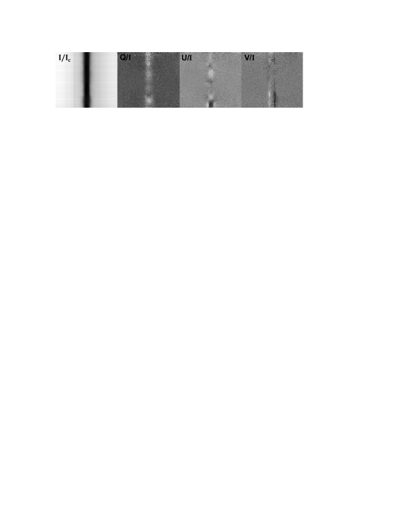
Figure 3: An example of our recent spectropolarimetric observations of the Ca II 8542 Å line in a very quiet region close to the solar limb, using ZIMPOL at the French-Italian telescope THEMIS. The reference direction for Stokes $Q$ is the tangent to the closest limb. From Trujillo Bueno et al. (2009).

Figure 3 shows a high-sensitivity spectropolarimetric observation of the quiet solar chromosphere in the strongest (8542 Å) line of the Ca II IR triplet. It was obtained by R. Ramelli (IRSOL), R. Manso Sainz (IAC) and me using the Zürich Imaging Polarimeter (ZIMPOL) attached to THEMIS. The observed Stokes $V/I$ profiles are clearly caused by the longitudinal Zeeman effect, while the Stokes $Q/I$ and $U/I$ signals are produced mainly by the influence of atomic level polarization. As seen in Fig. 3, although the spatio-temporal resolution of this spectropolarimetric observation is rather low (i.e., no better than $3\hbox{${}^{\prime\prime}$}$ and 20 minutes), the fractional polarization amplitudes fluctuate between 0.01% and 0.1% along the spatial direction of the spectrograph’s slit, with a typical spatial scale of $5\hbox{${}^{\prime\prime}$}$. Interestingly enough, while the Stokes $Q/I$ signal changes its amplitude but remains always positive along that spatial direction, the sign of the Stokes $U/I$ signal fluctuates.

The physical interpretation of this type of spectropolarimetric observations requires solving the non-LTE problem of the $2^{\rm nd}$ kind for the Ca II IR triplet. Fig. 4 shows examples of the emergent fractional linear polarization calculated with MULTIPOL in a semi-empirical model of the solar atmosphere. The top panels show the emergent $Q/I$ profiles for a LOS with $\mu=0.1$, for the unmagnetized reference case and for three possible orientations of a 5 mG horizontal magnetic field. The bottom panels show the corresponding $U/I$ signals, which are of course zero for the unmagnetized case. Note that while the amplitudes of the theoretical $Q/I$ profiles change with the strength and orientation of the magnetic field and are always positive, the sign of $U/I$ is sensitive to the azimuth of the magnetic field vector. Therefore, as expected, the spatial variations in the observed fractional linear polarization (see Fig. 3) are mainly due to changes in the orientation of the chromospheric magnetic field.

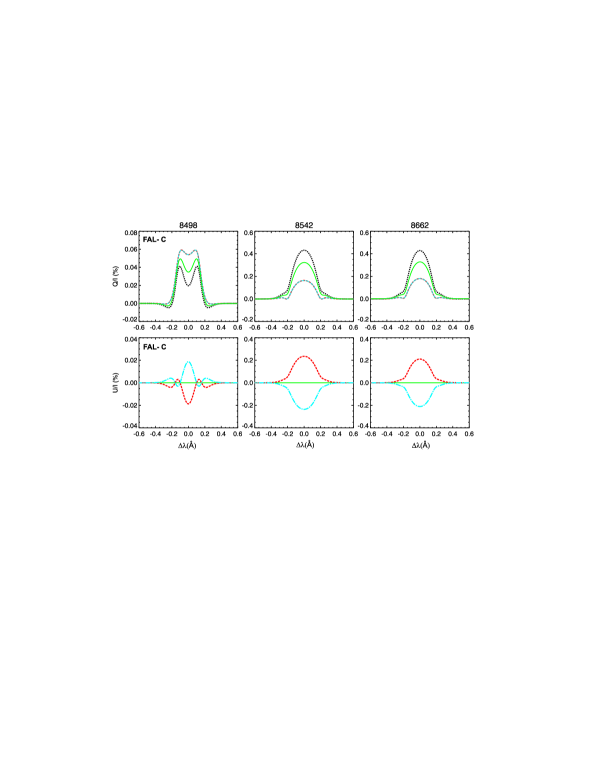
Figure 4: The emergent fractional linear polarization of the Ca II IR triplet calculated for a LOS with $\mu=0.1$ in a semi-empirical model of the solar atmosphere. For the $B=0$ case (dotted curves) only $Q/I$ is non-zero. The other curves refer to a horizontal 5 mG magnetic field pointing towards the observer (red dashed curves), perpendicular to the observer (green solid curves) and away from the observer (blue dash-dotted curves). The reference direction for Stokes $Q$ is the parallel to the closest limb. Note that while the $Q/I$ amplitude fluctuates but remains always positive, the sign of $U/I$ depends on the azimuth of the magnetic field. From Manso Sainz & Trujillo Bueno (2009b).

These types of polarization signal resulting from atomic level polarization and the Hanle and Zeeman effects can be exploited to explore the thermal and magnetic structure of the solar chromosphere. They can also be used to evaluate the degree of realism of magneto-hydrodynamic simulations of the photosphere-chromosphere system via careful comparisons of the observed Stokes profiles with those obtained through forward-modeling calculations.

6 Plasma structures in the chromosphere and corona

As mentioned above, a suitable diagnostic window for inferring the magnetic field vector of plasma structures embedded in the solar atmosphere is that provided by the polarization produced by the joint action of atomic level polarization and the Hanle and Zeeman effects in the He I 10830 Å and 5876 Å multiplets.

The resolved components of both helium multiplets stand out in emission when observing off-limb structures at a given height above the visible limb. Since their respective spectral lines have different sensitivities to the Hanle effect, one would benefit from observing them simultaneously in spicules and prominences. At present, such simultaneous spectropolarimetric observations can be carried out with THEMIS and with the polarimeter SPINOR attached to the Dunn Solar Telescope. The main uncertainty with off-limb observations is that we do not know whether the observed plasma structure was really in the plane of the sky during the observing period (i.e., it is not known whether the observed Stokes profiles were produced in 90^∘ scattering geometry or not).

Concerning on-disk observations it is clear that the He I 10830 Å triplet is the most suitable one, given that it shows significantly more absorption than the He I D₃ multiplet when observing a variety of plasma structures against the bright background of the solar disk. The additional fact that the Hanle effect in forward scattering creates measurable linear polarization signals in the lines of the He I 10830 Å multiplet when the magnetic field is inclined with respect to the local solar vertical direction (Trujillo Bueno et al. 2002b), and that there is a nearby photospheric line of Si I, makes the 10830 Å spectral region very suitable for investigating the coupling between the photosphere and the corona. The main uncertainty with on-disk observations is that we do not know the exact height above the solar visible surface where the observed plasma structure is located.

6.1 Off-limb diagnostics of prominences and spicules

The off-limb observational strategy consists in doing spectropolarimetric observations with the image of the spectrograph’s slit at given, ideally consecutive distances from the visible solar limb. The Stokes profiles measured at each pixel (or after downgrading the original spatial resolution to increase the signal-to-noise ratio) are then used to obtain information on the strength, inclination and azimuth of the magnetic field vector via the application of Stokes inversion techniques like those discussed in §4.2. All published applications to the He I D₃ multiplet observations are based on the optically-thin plasma assumption (e.g., Landi Degl’Innocenti (1982), Casini et al. (2003), López Ariste & Casini (2005)), while some of the reported He I 10830 Å observations were interpreted taking into account radiative transfer effects through the constant-property slab model discussed in §4.2 (see Trujillo Bueno et al. (2002b), Trujillo Bueno et al. (2005b) and Asensio Ramos et al. (2008)).

For example, Casini et al. (2003) interpreted new spectropolarimetric observations of quiescent solar prominences in the He I D₃ multiplet via the application of a PCA inversion code (López Ariste & Casini (2002)) based on an extensive database of theoretical Stokes profiles. These profiles were calculated using the optically thin approximation, covering all the magnetic configurations and scattering geometries of interest. For one of the observed prominences Casini et al. (2003) provided two-dimensional maps of the inferred magnetic field vector. Such maps showed the surprising feature of areas reaching up to 80 G within a background of prominence plasma with predominantly horizontal fields having 10–20 G (see also Casini et al. (2005)). Paletou et al. (2001) and Trujillo Bueno et al. (2002b) also inferred prominence fields significantly stronger than those found by Leroy and collaborators (see Leroy (1989)). For a detailed He I 10830 Å investigation of the magnetic field vector in a polar-crown prominence see Merenda et al. (2006).

Concerning spicules, it is important to emphasize that the observation and theoretical modeling of the Hanle and Zeeman effects in such spike-like jet features provides a suitable tool for investigating the magnetism of the solar chromosphere. The paper by Centeno et al. (2009) discusses briefly the results that several researchers have obtained through the interpretation of off-limb observations and reports on a recent investigation based on the application of the inversion code HAZEL to He I 10830 Å spectropolarimetric observations of spicules in the quiet solar chromosphere. They find magnetic fields with $B\approx 40$ G in a localized area of the slit-jaw image, which could represent a possible lower value for the field strength of organized network spicules.

Very interesting He I D₃ observations of spicules are shown in Fig. 5. The Stokes profiles of the left panel correspond to a quiet region, while those of the right panel were observed close to an active region. Obviously, for the magnetic strengths of spicules (i.e., $B\mathrel{\hbox to0.0pt{\lower 3.5pt\hbox{$\sim$}\hss}\raise 1.5pt\hbox{$<$}}100$ G) the observed linear polarization is fully dominated by the selective emission processes that result from the atomic alignment of the upper levels of the 3d³D term, without any significant influence of the transverse Zeeman effect. Note that in both regions Stokes $U$ is non-zero, which is the observational signature of the Hanle effect of an inclined magnetic field. The change of sign in Stokes $U$ along the spatial direction of the spectrograph’s slit can be easily explained by variations in the azimuth of the magnetic field vector. In contrast, the circular polarization profiles of the D₃ multiplet are the result of the joint action of the longitudinal Zeeman effect and of atomic level orientation (see §2). Interestingly, the Stokes $V$ profiles corresponding to the observed quiet region are dominated by atomic level orientation, while those observed in the spicules close to the active region are caused mainly by the longitudinal Zeeman effect.

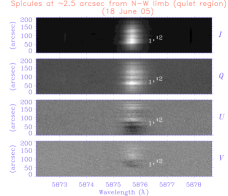
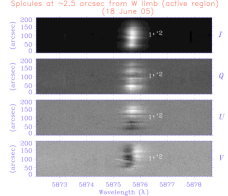
Figure 5: Illustrative examples of the off-limb Stokes profiles of the He I 5876 Å multiplet observed in a quiet region (left panels) and close to an active region (right panels). Interestingly, the inferred magnetic field vector has $B\approx 10$ G in the quiet region, while a best fit to the profiles observed close to the active region requires $B\approx 50$ G. The reference direction for Stokes $Q$ is the parallel to the solar limb. From Ramelli et al. (2006).

6.2 On-disk diagnostics of filaments

A significant difference between quiet region (QR) filaments and active region (AR) filaments is that the former are weakly magnetized (i.e., with $B<100$ G) and embedded in the $10^{6}$ K solar corona, while the latter are strongly magnetized (i.e., with $100\,{\rm G}\mathrel{\hbox to0.0pt{\lower 3.5pt\hbox{$\sim$}\hss}\raise 1.5pt\hbox{$<$}}B\mathrel{\hbox to0.0pt{\lower 3.5pt\hbox{$\sim$}\hss}\raise 1.5pt\hbox{$<$}}1000$ G) and located at much lower heights above the solar visible surface.

For magnetic strengths $B\mathrel{\hbox to0.0pt{\lower 3.5pt\hbox{$\sim$}\hss}\raise 1.5pt\hbox{$<$}}100$ G the linear polarization of the He I 10830 Å triplet is fully dominated by the atomic level polarization that is produced by anisotropic radiation pumping (Trujillo Bueno et al. (2002b)). For stronger magnetic fields, the contribution of the transverse Zeeman effect cannot be neglected. However, in principle, the emergent linear polarization should still show an important contribution caused by the presence of atomic level polarization, even for the unfavorable case of low-lying plasma structures having magnetic field strengths as large as 1000 G (see Fig. 2 in Trujillo Bueno & Asensio Ramos 2007; see also Fig. 2 of §4.2). Surprisingly, at the Fourth International Workshop on Solar Polarization V. Martínez Pillet and collaborators reported that the Stokes $Q$ and $U$ profiles of the He I 10830 Å multiplet from an active-region filament had the typical shape of polarization profiles produced by the transverse Zeeman effect. Such observations of an AR filament on top of a dense plage region at the polarity inversion line (i.e., an “abutted” plage region) have been recently analyzed in detail by Kuckein et al. (2009), showing that the filament magnetic fields were mainly horizontal and with strengths between 600 and 700 G. Figure 6 shows another example of Stokes profiles dominated by the Zeeman effect, observed in a (low-lying) filament in an AR with large sunspots.

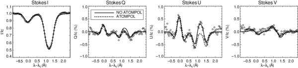
Figure 6: Example of Stokes profiles dominated by the Zeeman effect observed in an AR filament. Both best fits obtained with HAZEL give $B\approx 750$ G and $\theta_{B}=97^{\circ}$. This figure results from an ongoing collaboration with Y. Katsukawa (NAOJ).

What is the explanation of this enigmatic finding? According to Trujillo Bueno & Asensio Ramos (2007), the AR filament analyzed by Kuckein et al. (2009) had significant optical thickness so that the radiation field generated by the structure itself reduced the positive contribution to the anisotropy factor caused by the radiation from the underlying solar photosphere (see Fig. 4 of Trujillo Bueno & Asensio Ramos (2007)). At meaningful optical thickness in the “horizontal” direction (e.g., along the filament axis), the amount of atomic level alignment in the filament can be significantly reduced, to the extent that the transverse Zeeman effect of its strong horizontal field dominates the emergent linear polarization (e.g., a vertical light beam of intensity $I_{c}$ and two oppositely directed horizontal beams of intensity $I_{\rm filament}=S=I_{c}/4$ produce zero anisotropy in the horizontal reference system). An alternative possibility, suggested by Casini et al. (2008), requires the presence of a randomly oriented field entangled with the main filament field, and of similar magnitude (700 G!).

Another important question is whether all AR filaments permeated by a significantly strong (e.g., $B\approx 500$ G) and predominantly horizontal magnetic field show linear polarization profiles dominated by the transverse Zeeman effect. The fact that the answer to this question is negative can be seen in Fig. 7, which shows an example of the Stokes profiles that A. Asensio Ramos (IAC), C. Beck (IAC) and I observed on June 9, 2007 in an AR filament several hours before its eruption. The solid curves in the upper panels show the best theoretical fits to the observed Stokes profiles that the inversion code HAZEL gives when only the Zeeman effect is considered, while the lower panels demonstrate that the fit to the observed linear polarization is dramatically improved when the influence of atomic level polarization is also taken into account. It is interesting to note that, while the inferred inclination of the magnetic field with respect to the local vertical is $\theta_{B}\approx 115^{\circ}$ in both cases, the magnetic field strength turns out to be 70 G stronger when Stokes inversion is performed neglecting atomic level polarization.

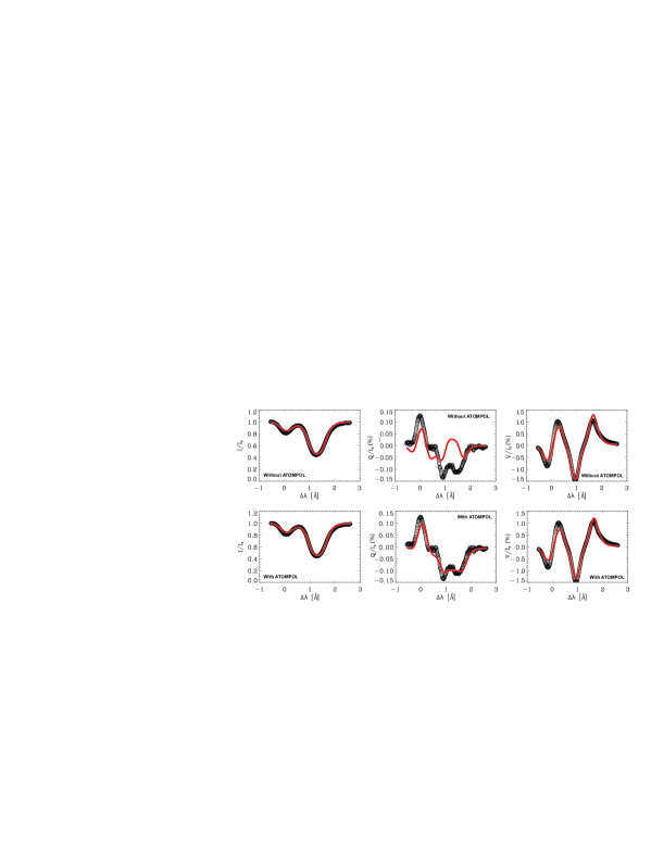
Figure 7: Example of the Stokes profiles observed in an AR filament a few hours before its eruption, using the Tenerife Infrared Polarimeter attached to the German VTT. Upper panels: the best theoretical fit obtained with HAZEL when neglecting atomic level polarization corresponds to $B=460$ G. Lower panels: the best theoretical fit when atomic level polarization is taken into account corresponds to $B=390$ G. In both cases the inferred inclination is $\theta_{B}=115^{\circ}$. The Stokes $U$ profile (not shown here) is more or less similar to the observed Stokes $Q$, but of opposite sign.

As seen in Fig. 7 the intensity profiles observed in this AR filament show significant absorption, which implies that the slab’s optical thickness along the LOS needed to fit them with HAZEL is significant. Therefore, following Trujillo Bueno & Asensio Ramos (2007), one may argue that the anisotropy of the radiation field within the filament was small and that, accordingly, the emergent linear polarization should be dominated by the transverse Zeeman effect. However, this was not the case (see the Stokes $Q$ panels of Fig. 7). I believe that the solution to this enigma has to do with the degree of compactness of the multitude of individual magnetic fibrils, stacked one upon another, that together determine the structure of a filament. Very likely, the plasma of the AR filament analyzed by Kuckein et al. (2009) had a high degree of compactness, such that a single constant-property slab or tube model with a significant optical thickness in the horizontal direction provides a suitable representation. As a result, the radiation field generated by the plasma structure itself may have produced a negative contribution to the anisotropy factor, so that the anisotropy of the true radiation field that illuminated the helium atoms in the filament body was significantly smaller than that corresponding to the optically thin case (see Fig. 4 of Trujillo Bueno & Asensio Ramos (2007)). On the contrary, in my opinion, a more suitable model for the AR filament we observed on June 9, 2007 a few hours before its eruption is that of a multitude of optically thin threads of magnetized plasma, each of them illuminated by the anisotropic radiation coming from the underlying photosphere, and such that the total optical thickness along the LOS is that needed by HAZEL to fit the observed Stokes $I(\lambda)$ profiles. The observational and theoretical support in favour of prominence thread structure is overwhelming (e.g., the review by Heinzel (2007)), but it is interesting to note that the signature of atomic level polarization in the linear polarization profiles observed in some AR filaments may provide information on the degree of compactness of the structure that results from the agglomeration of multitude of individual magnetized fibrils.

Finally, it is of interest to mention that on 11 September 2003 Merenda et al. (2007) carried out He I spectropolarimetric observations of a filament in a moderately active region that was located relatively close to the solar disk center, and found that the Stokes $Q$ and $U$ profiles were dominated by the influence of atomic level polarization in most of the filament body, except in a small region of the filament apparently close to one of its footpoints (where the observed linear polarization clearly resulted from the joint action of atomic level polarization and the transverse Zeeman effect). A detailed interpretation of these observations via the Stokes inversion strategy described in Merenda et al. (2006) allowed us to infer a full magnetic map of the filament, with the azimuth, inclination and strength of the magnetic field vector at each point within the filament (see Merenda et al. (2007) and Merenda (2008)). Interestingly, while the inferred magnetic field vector was predominantly horizontal, practically aligned with the local filament axis and with $B\approx 100$ G in most points of the filament body, it was found to be significantly stronger (a few hundred gauss) in the part of the filament apparently close to one of its footpoints.

6.3 Magnetic field “reconstruction” in emerging flux regions

Figure 8 shows results from spectropolarimetric measurements of a region with small pores observed in the 10830 Å spectral region. The left panel is a continuum image of the observed field of view, while the bright features in the right panel show the pixels where the equivalent width of the Stokes $I(\lambda)$ profile of the He I 10830 Å red blended component was significant. This is one of the most spectacular He I 10830 Å equivalent width images I have ever seen. It shows loop-like structures in an emerging flux region with the largest equivalent width values localized at the apex of the loops.

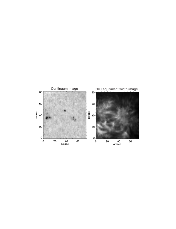
Figure 8: Observation of a region with small pores obtained in collaboration with M. Collados (IAC) using the Tenerife Infrared Polarimeter attached to the VTT.

It is not obvious to identify loops in the equivalent width image of the region observed by Solanki et al. (2003). In a recently published research note Judge (2009) has pointed out that if there were really loops in the region analyzed by Solanki et al. (2003) they must have been near the plane containing the loop footpoints and the LOS, otherwise their loop images would have appeared significantly curved. The conclusion by Solanki et al. (2003) that their data demonstrate the presence of a current sheet in the upper solar atmosphere is based on the assumption that the observed absorption in the He I 10830 Å triplet forms along magnetic field lines, which allowed them to associate a formation height to the magnetic field vector inferred at each pixel via the application of their Milne-Eddington inversion code. Judge (2009) has criticized this assumption on which the magnetic field “reconstruction” technique of Solanki et al. (2003) is based. He argues that He I 10830 Å formation along a horizontal slab is a more reasonable assumption that along the skin of the emerging flux region and that the magnetic field reconstructions by Solanki et al. (2003) lead to spurious results. I think, however, that the He I equivalent width image of Fig. 8 supports Solanki et al.’s assumption that in regions of emerging flux the He I triplet is formed within loops, but it is not clear to me whether “freshly emerged loops” were really present in the region they observed. Fortunately, it seems clear that loops were really present in the region corresponding to Fig. 8. Hence, we will soon try to invert the ensuing data with HAZEL in order to check carefully if the application of the reconstruction technique of Solanki et al. (2003) leads to loops coinciding with those seen in Fig. 8. This is important because, as far as I know, the magnetic field reconstruction technique proposed by Solanki et al. (2003) is the only available to deliver three-dimensional information about the magnetic field vector from He I 10830 Å spectropolarimetry.

7 How to map the magnetic fields of coronal loops ?

The primary emission of the $10^{6}$ K solar coronal plasma lies in the EUV and soft X-rays, two spectral regions that can only be observed from space. At such short wavelengths the coronal magnetic fields are unable to produce any significant Zeeman polarization signal. Therefore, a key question is: can we expect scattering polarization in permitted lines at EUV wavelengths for which the underlying quiet solar disk is seen completely dark? Manso Sainz & Trujillo Bueno (2009a) think that the answer is yes for the following reasons. For some EUV lines their lower level is the ground level of a forbidden line at visible or near-IR wavelengths, which is polarized due to the anisotropic illumination of the atoms at the forbidden line wavelength. This lower-level atomic alignment is transferred to the upper level of the EUV line by collisional excitation. Therefore, since the upper level of the EUV line can be polarized, we may have measurable scattering polarization signals caused by the ensuing selective emission processes in the allowed EUV line. The linear polarization thus generated would be sensitive to the electronic density ($N_{\rm e}$) and to the orientation of the magnetic field vector, although not to its strength because for permitted EUV lines $B\gg B_{\rm H}(J_{l})$ and $B\ll B_{\rm H}(J_{u})$ (with $B$ the magnetic strength in the coronal plasma). Interestingly enough, contrary to the case of forbidden line polarimetry (e.g., Casini & Judge (1999), Tomczyk et al. (2008)), such linear polarization in allowed EUV transitions would be observable also in forward scattering at the solar disk center. This is extremely important because it provides a way for mapping the magnetic field of the extended solar atmosphere all the way up from the photosphere to the corona.

There are several interesting EUV lines satisfying these requirements. For example, the theoretical prediction of Manso Sainz & Trujillo Bueno (2009a) for the Fe X line at 174.5 Å is that the ensuing $Q/I$ amplitude in $90^{\circ}$ scattering geometry at a height of 0.1 solar radii above the solar surface varies between about $0.1\%$ for $N_{\rm e}=10^{9}$ cm^-3 and $5\%$ for $N_{\rm e}=10^{7}$ cm^-3, being a factor two smaller for the case of a horizontal magnetic field observed against the solar disk in forward-scattering geometry.

8 Concluding comments

We should put high-sensitivity spectropolarimeters on ground-based and space telescopes for simultaneously measuring the polarization in photospheric and chromospheric lines. A very good choice would be the spectral region of the IR triplet of Ca II and/or that of the He I 10830 Å triplet. If, in addition, we want to do something technologically challenging, we could then put a EUV imaging polarimeter on a space telescope (i.e., a TRACE-like instrument, but capable of obtaining also linear polarization images of coronal loops).

It would also be of great scientific interest to put a high-sensitivity spectropolarimeter in space in order to simply discover what the linearly polarized UV spectrum of the Sun looks like. For example, lines like Mg II k at 2795 Å and the Ly ${\alpha}$ and Ly ${\beta}$ lines of hydrogen are expected to show measurable linear polarization signals, also when pointing at the solar disk center where we observe the forward scattering case (Trujillo Bueno et al. (2005a)). Such observations would provide precious information on the magnetic field structuring of the solar transition region from the chromosphere to the $10^{6}$ K solar coronal plasma.

Concerning improvements in the diagnostic tools of chromospheric and coronal fields, our next step will be to acknowledge that “the Sun is a wolf in sheep’s clothing” and to generalize the methods reported here to consider more sophisticated radiative transfer models and to account for variations of the magnetic fields and flows at sub-resolution scales. In fact, although many of the Stokes profiles observed in chromospheric lines can be fitted with one-component models, some of the observations discussed in this review and many others (e.g., Socas-Navarro et al. (2000a), Centeno et al. (2005), Lagg et al. (2007), Sasso et al. (2007)) indicate the need to consider at least two magnetic field components with different flows and/or orientations.