Discrete Inverse Scattering Theory for NMR Pulse Design

Chapter 1 Introduction

The problem of selective excitation pulse design in nuclear magnetic resonance (NMR) corresponds, in mathematics, to the inversion of a certain mapping, $\mathcal{T}$, which we call the selective excitation transform. This transform, which is a kind of non-linear Fourier transform, maps complex-valued functions of time, called pulses, to unit $3$-vector valued functions of frequency, called magnetization profiles. The explicit definition of $\mathcal{T}$ is given in Section 1.1. The theory of inverting $\mathcal{T}$ has been shown to coincide with the theory of inverse scattering for the Zakharov-Shabat (ZS) $2\times 2$ system (see Section 2.2 and for example [14]). Numerous authors have studied this inverse scattering problem, for example Ablowitz et al. [1], and the results have been applied to NMR pulse design (see for example [14, 3]). However, no stable and efficient algorithm has been given in the literature for generating the full space of solutions to the inverse problem. For this and other reasons, less exact methods for NMR pulse design, such as the Fourier transform method and the Shinnar-Le Roux (SLR) method, have been used in practice instead of the more exact and more flexible inverse scattering (IST) method. In this thesis, we present the discrete inverse scattering transform (DIST) algorithm for efficiently solving the full inverse scattering problem relating to NMR pulse design.

In this introductory chapter, we define the continuum and discrete selective excitation transforms and describe the problem of selective excitation pulse design. The theoretical results are summarized in Sections 1.5, 1.6, and 1.7, and the main algorithms are described in Section 1.8.

The second chapter is devoted to proving the main theorems and deriving the algorithms. We introduce the discrete scattering theory, which is completely analogous to the standard continuum theory.

The third chapter describes how to apply the theory to practical NMR pulse design.

See [4] and [5] for a detailed mathematical introduction to NMR imaging and NMR pulse design.

1.1. The selective excitation transform

In this section we define the selective excitation transform, which maps a complex function of time to a unit $3$-vector valued function of frequency.

Let $\omega:\mathbb{R}\rightarrow\mathbb{C}$ be a function of time (usually we think of $\omega$ as smooth and supported on a finite interval), and suppose that for every frequency $z\in\mathbb{R}$, there is a solution $M_{-}(z;\cdot):\mathbb{R}\rightarrow\mathbb{R}^{3}$ to the frequency dependent Bloch equation (without relaxation)

(1.1.1) $$\frac{d}{dt}M_{-}(z;t)=M_{-}(z;t)\times\left[\begin{array}[]{c}\text{Re }\omega(t)\\ \text{Im }\omega(t)\\ z\end{array}\right]$$

normalized by

(1.1.2) $$\lim_{t\rightarrow-\infty}M_{-}(z;t)=\left[\begin{array}[]{c}0\\ 0\\ 1\end{array}\right].$$

Let us show that such a solution is unique. If $M_{1}$ and $M_{2}$ are two solutions to (1.1.1) then $M_{1}(z;t)^{T}M_{2}(z;t)$ is independent of $t$ because

$$\frac{d}{dt}M_{1}(z;t)^{T}M_{2}(z;t) = \left[X_{B}(z;t)M_{1}(z;t)\right]^{T}M_{2}(z;t)+M_{1}(z;t)^{T}\left[X_{B}(z;t)M_{2}(z;t)\right]$$

$$= M_{1}^{T}(z;t)\left(X_{B}(z;t)^{T}+X_{B}(z;t)\right)M_{2}(z;t)$$

$$= 0,$$

where

$$X_{B}(z;t)=\left[\begin{array}[]{ccc}0&z&-\text{Im }\omega(t)\\ -z&0&\text{Re }\omega(t)\\ \text{Im }\omega(t)&-\text{Re }\omega(t)&0\end{array}\right].$$

Therefore, (1.1.2) implies that $M_{-}(z;t)^{T}M_{-}(z;t)=1$. So $M_{-}(z;t)$ is a unit vector for all $z$ and $t$. It is unique because, if $M_{2}(z;t)$ is any unit vector satisfying $M_{-}(z;t)^{T}M_{2}(z;t)=1$, then the Cauchy-Schwarz inequality implies that $M_{-}(z;t)=M_{2}(z;t)$.

Suppose that $\omega$ decays sufficiently so that

$$\mathbf{M}(z):=\lim_{t\rightarrow+\infty}\left[\begin{array}[]{ccc}\text{Re }e^{izt}&-\text{Im }e^{izt}&0\\ \text{Im }e^{izt}&\text{Re }e^{izt}&0\\ 0&0&1\end{array}\right]M_{-}(z;t)$$

exists for all $t$. For example, this limit exists whenever $\omega$ is integrable (see [5]). We call $\omega$ the pulse and $\mathbf{M}$ the resulting magnetization profile. The map $\omega\mapsto\mathbf{M}$ is called the selective excitation transform, and we write $\mathbf{M}=\mathcal{T}\omega$. In Section 1.3 we plot several examples of pulses and their resulting magnetization profiles.

1.2. The problem of selective excitation pulse design

In selective excitation pulse design, we usually start with an ideal magnetization profile $\mathbf{M}_{\textrm{ideal}}:\mathbb{R}\rightarrow S^{2}\subset\mathbb{R}^{3}$. This is a unit 3-vector valued function of frequency which is typically equal to $\left[\begin{array}[]{ccc}0&0&1\end{array}\right]^{t}$ outside some finite interval. The problem is to find a pulse $\omega:\mathbb{R}\rightarrow\mathbb{C}$ such that the resulting magnetization profile $\mathbf{M}=\mathcal{T}\omega$ is a good approximation to $\mathbf{M}_{\textrm{ideal}}$. For practical applications, $\omega$ should have finite duration. That is, it should be supported in some finite interval $[\rho-T,\rho]\subset\mathbb{R}$. The number $T$ is called the duration of the pulse, and the value $\rho$ is called the rephasing time. Depending on the application, it may be important to design a pulse with the shortest possible duration and minimal (perhaps zero) rephasing time (pulses with $\rho=0$ are called self refocused). It is also often necessary to limit the energy

$$E_{\omega}:=\int_{-\infty}^{\infty}\left|\omega(t)\right|^{2}dt$$

of the pulse, as well as the maximum amplitude. For many application it is important that the pulse behaves well under imperfect magnetic field conditions. That is, $\frac{\partial\mathbf{M}}{\partial\omega}$ should not be too large.

The standard example of an ideal magnetization profile is

$$M_{ideal}(z)=\begin{cases}\left[\begin{array}[]{c}0\\ \sin\theta_{0}\\ \cos\theta_{0}\end{array}\right]&\textrm{if }|z-z_{0}|<c_{0}\\ \\ \left[\begin{array}[]{c}0\\ 0\\ 1\end{array}\right]&\textrm{if }|z-z_{0}|>c_{0}.\end{cases}$$

Here, the magnetization is rotated $\theta_{0}$ radians around the $x$-axis for frequencies in the interval $|z-z_{0}|<c_{0}$. Outside of this frequency interval, the magnetization is kept at equilibrium. The angle $\theta_{0}$ is called the flip angle. See the next section and Chapter 3 for plots of pulses producing magnetization profiles that approximate such a profile.

1.3. Examples

When $\int_{-\infty}^{\infty}|\omega(t)|dt$ is small, the resulting magnetization profile $\mathbf{M}=\mathcal{T}\omega$ very closely resembles the Fourier transform of $\omega$ (see for example [5]). This fact is illustrated in Figures 1.3.1 and 1.3.2. Figure 1.3.1 shows a pulse which is constant over a finite interval. Notice that at zero frequency, the magnetization is rotated $\frac{\pi}{2}$ radians around the $x$-axis, and away from zero the transverse magnetization resembles a sinc function. Figures 1.3.2 and 1.3.3 show truncated sinc pulses. Such pulses are often used in practice to produce a magnetization profile which is approximately constant within some finite interval, and approximately in equilibrium outside the interval. Notice that as the flip angle increases from $90^{\circ}$ to $120^{\circ}$, the resulting magnetization profile does a worse job approximating the ideal.

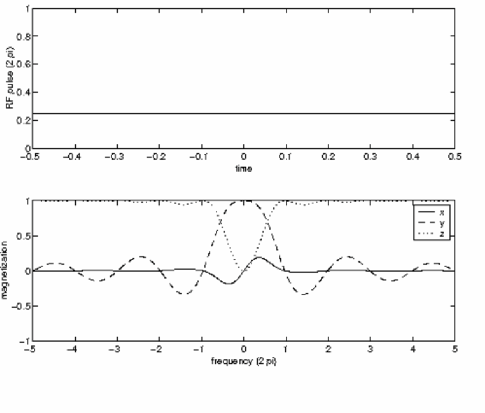
Figure 1.3.1. A constant pulse and the resulting magnetization: $T=1,$ $\rho=\frac{1}{2}$.

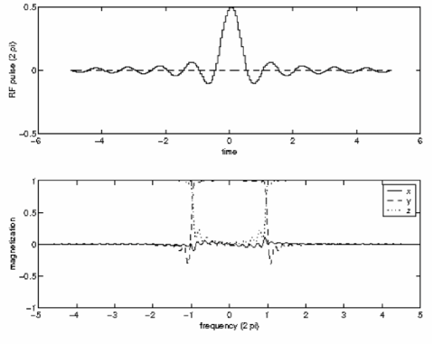
Figure 1.3.2. A $90^{\circ}$ sinc pulse and the resulting magnetization: N=10, $\rho\approx 5$.

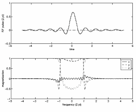
Figure 1.3.3. A $120^{\circ}$ sinc pulse and the resulting magnetization: N=10, $\rho\approx 5$.

To obtain a more accurate magnetization profile, one should invert the selective excitation transform directly rather than use the Fourier transform approximation. Figures 1.3.4, 1.3.5, and 1.3.6 show three very different pulses which produce magnetization profiles which accurately approximate a $120^{\circ}$ profile. The fact that the inversion of the selective excitation transform is highly non-unique reflects the nonlinearity of the map $\omega\mapsto\mathcal{T}\omega$.

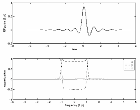
Figure 1.3.4. A $120^{\circ}$ minimum energy pulse and the resulting magnetization.

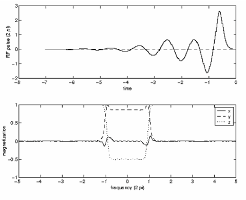
Figure 1.3.5. A $120^{\circ}$ self refocused pulse.

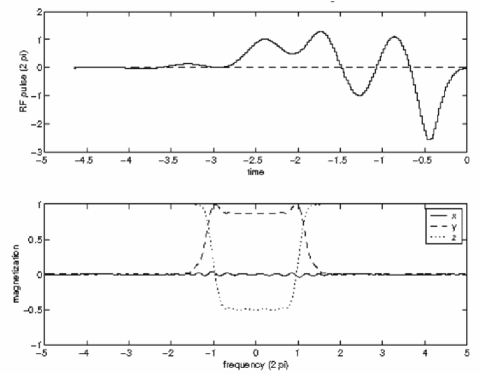
Figure 1.3.6. A $120^{\circ}$ self refocused pulse.

1.4. The discrete selective excitation transform (hard pulse approximation)

For practical purposes it is useful to consider pulses of the form

$$\Omega(t)=\sum_{j=-\infty}^{\infty}\omega_{j}\delta(t-j\Delta).$$

For example, this is the type of pulse designed by the SLR algorithm (see [12]). Such a pulse is called a hard pulse. If $\omega_{j}$ vanishes for all $j\geq\rho\in\mathbb{Z}$, then $\Omega$ is said to have $\rho$ rephasing time steps. In practical applications, a softened version, e.g.,

(1.4.1) $$\Omega_{\epsilon}(t)=\sum_{j=-\infty}^{\infty}\frac{\omega_{j}}{\epsilon}\chi_{[0,\epsilon)}(t-j\Delta)$$

is typically used. The energy of the softened pulse is

(1.4.2) $$E_{\Omega_{\epsilon}}=\epsilon^{-1}\sum_{j=-\infty}^{\infty}|\omega_{j}|^{2},$$

which tends to infinity as $\epsilon\rightarrow 0$. We think of the hard pulse as an ideal non-physical pulse corresponding to $\epsilon=0$. In Appendix B, we explore the relationship between the hard and softened pulses.

For a pulse of the form (1.4.1), it is possible solve the Bloch equation (1.1.1) explicitly. In the limit, as $\epsilon$ approaches $0$, the Bloch equation can be replaced by the recursion

$$M_{-}(z;(j+1)\Delta)=P_{\Delta}R_{\omega_{j}}M_{-}(z;j\Delta),$$

where $P_{\Delta}$ corresponds to a certain frequency-dependent rotation around the z-axis, and $R_{\omega_{j}}$ corresponds to a certain frequency-independent rotation around the $\left[\begin{array}[]{c}\text{Re }\omega_{j}\\ \text{Im }\omega_{j}\\ 0\end{array}\right]$-axis. The precise definitions of the operators $P_{\Delta}$ and $R_{\omega_{j}}$ are given in Section 2.4.

For hard pulses, we evaluate the magnetization $M_{-}$ only at the discrete time points $j\Delta$ for $j\in\mathbb{Z}$. It is easy to see that, at such time points, $M_{-}$ is a periodic function of the frequency – it is a function of $w=e^{i\Delta z}$. We suppress the dependence on $\Delta$ and $z$ and write $M_{-}=M_{-}(w;j)$ as a function of $w\in S^{1}$ and $j\in\mathbb{Z}$. The resulting magnetization profile is

$$\mathbf{M}(w):=\lim_{j\rightarrow\infty}P_{\Delta}^{-j}M_{-}(w;j),$$

a function on $S^{1}$. We define the discrete selective excitation transform by

$$\mathcal{T}^{\textrm{disc}}\Omega:=\mathbf{M}=\lim_{j\rightarrow\infty}P_{\Delta}^{-j}M_{-}(\cdot;j).$$

A condition on $\Omega$ that guarantees the existence of this limit is given in Section 2.5. The transform $\mathcal{T}^{\textrm{disc}}$ maps hard pulses (sequences of complex numbers) to periodic magnetization profiles ($S^{2}$ valued functions on $S^{1}$).

1.5. Main results: continuum theory

The problem of inverting the selective excitation transform has been solved using inverse scattering theory. We prove in Section 2.12

Theorem 1.5.1.

Let $\mathbf{M}=\left[\begin{array}[]{c}\mathbf{M}_{x}\\ \mathbf{M}_{y}\\ \mathbf{M}_{z}\end{array}\right]:\mathbb{R}\rightarrow S^{2}\subset\mathbb{R}^{3}$ be a magnetization profile, and set

$$r(\xi)=\frac{\mathbf{M}_{x}(2\xi)+i\mathbf{M}_{y}(2\xi)}{1+\mathbf{M}_{z}(2\xi)}.$$

Assume that $r$ and $\xi r$ are in $H^{1}(\mathbb{R})$.
(a) There are infinitely many pulses $\omega$ such that $\mathcal{T}\omega=\mathbf{M}$. These pulses are parameterized by their bound state data (see below).
(b) If $r$ has the form $r(\xi)=e^{-2i\xi\rho}r_{0}(\xi)$ where $r_{0}$ has a meromorphic extension to the upper half plane with finitely many poles, and if

$$\lim_{|\xi|\rightarrow\infty}r_{0}(\xi)=0,$$

then there exists a pulse $\omega$ with rephasing time $\rho$ such that $\mathcal{T}\omega=\mathbf{M}$.
(c) Suppose that $r$ has the form $r(\xi)=e^{-2i\xi\rho}\frac{B(\xi)}{A(\xi)}$, for $A-1$ and $B$ in $H_{+}(\mathbb{R})$ (see Section 2.1.1) satisfying

$$|A(\xi)|^{2}+|B(\xi)|^{2}=1\textrm{ for all }\xi\in\mathbb{R},$$

and suppose that the Fourier transform of $B$ is supported on the interval $[0,2T]\subset\mathbb{R}$. Also assume that $A$ has an analytic extension to the entire complex plane. Then there exists a pulse $\omega$ with duration $T$ and rephasing time $\rho$ such that $\mathcal{T}\omega=\mathbf{M}$.

The function $r:\mathbb{R}\rightarrow\mathbb{C}$ is called the reflection coefficient. The magnetization profile $\mathbf{M}$ is uniquely determined by the reflection coefficient:

(1.5.1) $$\mathbf{M}(z)=\left[\begin{array}[]{c}\frac{2\text{Re }r}{1+|r|^{2}}\\ \frac{2\text{Im }r}{1+|r|^{2}}\\ \frac{1-|r|^{2}}{1+|r|^{2}}\end{array}\right](\frac{z}{2}).$$

The bound state data mentioned in part (a) of Theorem 1.5.1 is defined in Section 2.3. In the basic and generic case, this bound state data takes the form

$$D=(\xi_{1},\xi_{2},\dots,\xi_{m};C_{1}^{\prime},C_{2}^{\prime},\dots,C_{m}^{\prime}),$$

where $\xi_{1},\dots,\xi_{m}$ are distinct complex numbers in the upper half plane called energies, and $C_{1}^{\prime},\dots,C_{m}^{\prime}$ are non-zero complex numbers called norming constants. The main result is that to each such $r$ and $D$, there corresponds a unique pulse. The special case of no bound states ($m=0$) corresponds to a pulse called the minimum energy pulse (see [5]).

1.6. Main results: discrete theory

There is a completely analogous theory for the discrete selective excitation transform. The following Theorem is proved in Section 2.11.

Theorem 1.6.1.

Let $\mathbf{M}=\left[\begin{array}[]{c}\mathbf{M}_{x}\\ \mathbf{M}_{y}\\ \mathbf{M}_{z}\end{array}\right]:S^{1}\rightarrow S^{2}\subset\mathbb{R}^{3}$ be a periodic magnetization profile, and set

$$r=\frac{\mathbf{M}_{x}+i\mathbf{M}_{y}}{1+\mathbf{M}_{z}}.$$

Assume that $r$ is in $H^{1}(S^{1})$.
(a) There are infinitely many hard pulses $\Omega$ such that $\mathcal{T}^{\textrm{disc}}\Omega=\mathbf{M}$. These hard pulses are parameterized by their bound state data (see below).
(b) If $r$ has the form $r(w)=w^{-\rho}r_{0}(w)$ where $r_{0}$ has a meromorphic extension to the unit disk which vanishes at the origin, then there exists a hard pulse $\Omega$ with $\rho$ rephasing time steps such that $\mathcal{T}^{\textrm{disc}}\Omega=\mathbf{M}$.
(c) If $r$ has the form $r(w)=w^{-\rho}\frac{B(w)}{A(w)}$, where $A$ and $B$ are polynomials of degree $T$ which satisfy

$$|A(w)|^{2}+|B(w)|^{2}=1\textrm{ for all }w\in S^{1},$$

then there exists a hard pulse $\Omega$ with duration $T$ and $\rho$ rephasing time steps such that $\mathcal{T}^{\textrm{disc}}\Omega=\mathbf{M}$.

Again, $r:S^{1}\rightarrow\mathbb{C}$ is called the reflection coefficient, and the magnetization profile $\mathbf{M}$ can be obtained from the reflection coefficient using

(1.6.1) $$\mathbf{M}(w)=\left[\begin{array}[]{c}\frac{2\text{Re }r}{1+|r|^{2}}\\ \frac{2\text{Im }r}{1+|r|^{2}}\\ \frac{1-|r|^{2}}{1+|r|^{2}}\end{array}\right](w).$$

The bound state data mentioned in part (a) of Theorem 1.6.1 is defined in Section 2.4. In the basic and generic case, this bound state data takes the form

$$D=(w_{1},w_{2},\dots,w_{m};c_{1}^{\prime},c_{2}^{\prime},\dots,c_{m}^{\prime}),$$

where $w_{1},\dots,w_{m}$ are distinct complex numbers in the unit disk called energies, and $c_{1}^{\prime},\dots,c_{m}^{\prime}$ are non-zero complex numbers called norming constants. The main result is that to each such $r$ and $D$, there corresponds a unique hard pulse. The special case of no bound states ($m=0$) corresponds to a hard pulse called the minimum energy hard pulse. In Section 2.13, we discuss the relationship between the continuum bound state data and the discrete bound state data.

1.7. Energy Formulas

The following theorem is proved in [6]. The corollary is immediate (see Section 2.11).

Theorem 1.7.1.

Let $r$ be a reflection coefficient as in Theorem 1.5.1, and let $D=(\xi_{1},\xi_{2},\dots,\xi_{m};C_{1}^{\prime},C_{2}^{\prime},\dots,C_{m}^{\prime}),$ be bound state data. Then the energy of the corresponding pulse $\omega:\mathbb{R}\rightarrow\mathbb{C}$ is

$$E_{\omega}=\int_{-\infty}^{\infty}|\omega(t)|^{2}dt=\frac{4}{\pi}\int_{-\infty}^{\infty}\log(1+|r(\xi)|^{2})d\xi+16\sum_{k=1}^{m}\text{Im }\xi_{k}.$$

Corollary 1.7.2.

Let $r(\xi)=e^{-2i\xi\rho}r_{0}(\xi)$ be a reflection coefficient as in part (b) of Theorem 1.5.1, and let $\omega$ be the corresponding pulse with rephasing time $\rho$. Then the energy of $\omega$ is

(1.7.1) $$E_{\omega}=\int_{-\infty}^{\infty}|\omega(t)|^{2}dt=\frac{4}{\pi}\int_{-\infty}^{\infty}\log(1+|r(\xi)|^{2})d\xi+16\sum_{k=1}^{m}d_{k}\text{Im }\xi_{k},$$

where $\xi_{1},\dots,\xi_{m}$ are the poles of $r_{0}$ in the upper half plane, and $d_{1},\dots,d_{m}$ are the corresponding multiplicities.

The following theorem and its corollary are proved in Section 2.10.

Theorem 1.7.3.

Let $r$ be a reflection coefficient as in Theorem 1.6.1, and let $D=(w_{1},w_{2},\dots,w_{m};c_{1}^{\prime},c_{2}^{\prime},\dots,c_{m}^{\prime})$ be discrete bound state data. Let $\Omega(t)=\sum_{j=-\infty}^{\infty}\omega_{j}\delta(t-j\Delta)$ be the corresponding hard pulse. Then

$$\sum_{j=-\infty}^{\infty}\log(1+\tan^{2}\frac{|\omega_{j}|}{2})=\frac{1}{2\pi}\int_{0}^{2\pi}\log(1+|r(e^{i\theta})|^{2})d\theta-2\sum_{k=1}^{m}\log|w_{k}|.$$

Corollary 1.7.4.

Let $r(w)=w^{-\rho}r_{0}(w)$ be a reflection coefficient as in part (b) of Theorem 1.6.1, and let $\Omega(t)=\sum_{j=-\infty}^{\rho}\omega_{j}\delta(t-j\Delta)$ be the corresponding pulse with $\rho$ rephasing time steps. Then

$$\sum_{j=-\infty}^{\infty}\log(1+\tan^{2}\frac{|\omega_{j}|}{2})=\frac{1}{2\pi}\int_{0}^{2\pi}\log(1+|r(e^{i\theta})|^{2})d\theta-2\sum_{k=1}^{m}d_{k}\log|w_{k}|,$$

where $w_{1},\dots,w_{m}$ are the poles of $r_{0}$ in the unit disk, and $d_{1},\dots,d_{m}$ are the corresponding multiplicities.

1.8. Algorithms

There are three main algorithms for producing hard pulses: the SLR algorithm, the finite rephasing time algorithm, and the DIST recursion.

1.8.1. The SLR algorithm

The SLR algorithm, discovered independently by M. Shinnar, and his co-workers, and P. Le Roux, can only be used to design hard pulses of finite duration, as in part (c) of Theorem 1.6.1. The input to the algorithm consists of the number of rephasing time steps, $\rho$, and the two polynomials $A$ and $B$ which must satisfy

(1.8.1) $$|A|^{2}+|B|^{2}=1$$

on the unit circle. The designed magnetization profile is determined using equation (1.5.1) with the reflection coefficient

$$r(w)=w^{-\rho}\frac{B(w)}{A(w)}.$$

The main drawback of this method is that one does not have direct control over the magnetization profile (more precisely, the phase of the reflection coefficient). On the other hand, one has complete control of the duration, which coincides with the degree of the polynomial $B$. The SLR technique uses the fact that the magnitude of $B$ is related to the $z$-component of the resulting magnetization profile $\mathbf{M}=\left[\begin{array}[]{c}\mathbf{M}_{x}\\ \mathbf{M}_{y}\\ \mathbf{M}_{z}\end{array}\right]$ by the formula

$$\mathbf{M}_{z}=\frac{1-|r|^{2}}{1+|r|^{2}}=|A|^{2}-|B|^{2}=1-2|B|^{2}.$$

The polynomial $B$ is designed so that $1-2|B|^{2}$ approximates the ideal $z$-magnetization, and then $A$ is chosen to satisfy equation (1.8.1) . The phase of the transverse magnetization $\mathbf{M}_{x}+i\mathbf{M}_{y}$ is not directly specified by this procedure, and ad hoc methods must be used to obtain a good approximation of the desired phase. This disadvantage is discussed further in Section 3.2.3 where we compare SLR pulses to inverse scattering pulses.

1.8.2. The finite rephasing time algorithm

The finite rephasing time algorithm resembles the SLR algorithm, but it is more flexible. It produces pulses of infinite duration, and finite rephasing time. Similar algorithms have been presented by various authors. See for example [16, 2].

The finite rephasing time algorithm can be used to produce the pulse from part (b) of Theorem 1.6.1. The input to this algorithm is the number of rephasing time steps, $\rho$, and a rational function $r_{0}=\frac{P}{Q}$, where $P$ and $Q$ are polynomials (possibly of very high degree). These polynomials do not need to satisfy any kind of equation like (1.8.1). The designed magnetization profile is determined using equation (1.5.1) with the reflection coefficient

$$r(w)=w^{-\rho}\frac{P(w)}{Q(w)}.$$

With this algorithm, one has direct control of the entire magnetization profile (not just the $z$-component as in the SLR algorithm), but control on the pulse duration is sacrificed. In fact, the designed pulse almost always has technically infinite duration. However, we will see in Chapter 3 that for many common applications, the effective duration of pulses designed with this method is within a reasonable range. The loss of direct control on the duration causes no disadvantage in practice.

This algorithm is more general than the SLR algorithm, and equally efficient. In Chapter 3 we give a simple derivation of the algorithm, and we describe several applications in NMR pulse design.

1.8.3. The DIST recursion

The discrete inverse scattering transform (DIST) algorithm, which we introduce in this thesis, efficiently handles the most general case of hard pulse design. It is motivated by the inverse scattering method of pulse design (see [5]). The input to the algorithm is called the scattering data and consists of:

(a) An arbitrary reflection coefficient, $r:S^{1}\rightarrow\mathbb{C}$;

(b) Arbitrary bound state data (see Section 2.4).

For technical reasons, we assume that $r$ is in $H^{1}(S^{1})$.

The derivation of this algorithm, and the proof that the output pulse has the correct scattering data is the main result of this thesis. This derivation and proof can be found in Chapter 2.

Chapter 2 Scattering theory

2.1. Preliminaries

2.1.1. The projection operators $\Pi_{+}$ and $\Pi_{-}$

The Paley-Wiener theorem states that every function $f\in L^{2}(\mathbb{R})$ can be written uniquely in the form

$$f=f_{+}+f_{-},$$

where $f_{+}\in L^{2}(\mathbb{R})$ has an analytic extension to the upper half plane, and $f_{-}\in L^{2}(\mathbb{R})$ has an analytic extension to the lower half plane satisfying

$$\lim_{|\xi|\rightarrow\infty}f_{\pm}(\xi)=0.$$

We define the projection operators $\Pi_{+},\Pi_{-}:L^{2}(\mathbb{R})\rightarrow L^{2}(\mathbb{R})$ by

$$(\Pi_{+}f)(\xi) = f_{+}(\xi)=\frac{1}{2\pi}\int_{0}^{\infty}\hat{f}(y)e^{i\xi y}dy$$

$$(\Pi_{-}f)(\xi) = f_{-}(\xi)=\frac{1}{2\pi}\int_{-\infty}^{0}\hat{f}(y)e^{i\xi y}dy.$$

Let $H_{+}(\mathbb{R})$ and $H_{-}(\mathbb{R})$ denote the ranges of $\Pi_{+}$ and $\Pi_{-}$, respectively.

Similarly, every function $f\in L^{2}(S^{1})$ can be written uniquely in the form

$$f=f_{0}+f_{+}+f_{-},$$

where $f_{0}\in\mathbb{C}$ is a constant, $f_{+}\in L^{2}(S^{1})$ has an analytic extension to the unit disk, vanishing at the origin, and $f_{-}$ has an analytic extension to $\hat{\mathbb{C}}\setminus\mathbb{D}$, vanishing at $\infty$. We define the operators $\Pi_{+},\Pi_{-},\tilde{\Pi}_{+},\tilde{\Pi}_{-}:L^{2}(S^{1})\rightarrow L^{2}(S^{1})$ by

$$(\Pi_{+}f)(w) = f_{+}(w)=\sum_{j=1}^{\infty}\hat{f}(j)w^{j}$$

$$(\Pi_{-}f)(w) = f_{-}(w)=\sum_{j=-\infty}^{-1}\hat{f}(j)w^{j}$$

$$\tilde{\Pi}_{+}f = f_{+}+\frac{1}{2}\hat{f}(0)$$

$$\tilde{\Pi}_{-}f = f_{-}+\frac{1}{2}\hat{f}(0).$$

Let $H_{+}$, $H_{-}$, $\tilde{H}_{+}$, and $\tilde{H}_{-}$ denote the ranges of $\Pi_{+}$, $\Pi_{-}$, $\tilde{\Pi}_{+}$, and $\tilde{\Pi}_{-}$, respectively.

The following lemma will be needed later in the chapter.

Lemma 2.1.1.

Suppose that $f$ is in $L^{2}(\mathbb{R})$ and that $\xi f$ is in $L^{2}(\mathbb{R})$. Then

(2.1.1) $$i\xi\Pi_{+}f-\Pi_{+}i\xi f=-\frac{1}{2\pi}\hat{f}(0),$$

and

(2.1.2) $$i\xi\Pi_{-}f-\Pi_{-}i\xi f=\frac{1}{2\pi}\hat{f}(0).$$

Proof.

First note that the hypothesis implies that $\hat{f}(0)$ is well defined. We will assume sufficient regularity and decay for $f$ so that the below integrals make sense. The general result then follows by continuity.

Integrating by parts gives

$$\frac{1}{2\pi}\int_{0}^{\infty}\hat{f}^{\prime}(t)e^{it\xi}dt+\frac{i\xi}{2\pi}\int_{0}^{\infty}\hat{f}(t)e^{it\xi}dt=-\frac{1}{2\pi}\hat{f}(0).$$

Notice that the first term on the left is $-\Pi_{+}i\xi f$ and the second term is $i\xi\Pi_{+}f$ . This proves (2.1.1). A similar computation can be used to prove (2.1.2). ∎

2.1.2. The reflection coefficient

Later in the chapter we will be working with functions of the form $r=\frac{b}{a}$ where $a$ and $b$ satisfy $|a|^{2}+|b|^{2}=1$ on $\mathbb{R}$. In this section we mention some results which are well known in the inverse scattering literature.

Proposition 2.1.2.

Let $r\in H^{1}(\mathbb{R})$, let $\xi_{1},\dots,\xi_{m}\in\mathbb{H}$, and let $d_{1},\dots,d_{m}$ be positive integers. Then there exist unique continuous functions $a,b:\mathbb{R}\rightarrow\mathbb{C}$ such that
(i) $r=\frac{b}{a}$ on $\mathbb{R}$;
(ii) $|a(\xi)|^{2}+|b(\xi)|^{2}=1$ for all $\xi\in\mathbb{R}$;
(iii) $a$ has an analytic extension to the upper half plane with zeros at $\xi_{1},\dots,\xi_{m}$ of orders $d_{1},\dots,d_{m}$;
(iv) $\lim_{|\xi|\rightarrow\infty}a(\xi)=1$.

Proof.

We need only consider the case where $a$ is non-vanishing ($m=0$), because adding zeros simply amounts to multiplying $a$ and $b$ by a common Blaschke product. Therefore, $\log a$ is an analytic function which, by condition (iv), must tend to $0$ at $\infty$. We know that

$$\text{Re }\log a=\log|a|=-\frac{1}{2}\log(1+|r|^{2}).$$

Notice that $\log(1+|r|^{2})$ is in $H^{1}(\mathbb{R})$. Therefore, we must have

$$\log a=-\Pi_{+}(1+|r|^{2}).$$

The general solution is

$$a=\prod_{k=1}^{m}\left(\frac{\xi-\xi_{k}}{\xi-\xi_{k}^{*}}\right)^{d_{k}}\cdot\exp(-\Pi_{+}(1+|r|^{2}))$$

and

$$b=ra.$$

∎

Proposition 2.1.3.

Let $r\in H^{1}(S^{1})$, let $w_{1},\dots,w_{m}\in\mathbb{D}$, and let $d_{1},\dots,d_{m}$ be positive integers. Then there exist unique continuous functions $a,b:S^{1}\rightarrow\mathbb{C}$ such that
(i) $r=\frac{b}{a}$ on $S^{1}$;
(ii) $|a|^{2}+|b|^{2}=1$ on $S^{1}$;
(iii) $a$ has an analytic extension to the unit disk with zeros at $w_{1},\dots,w_{m}$ of orders $d_{1},\dots,d_{m}$;
(iv) $a(0)>0$.

Proof.

The proof is essentially the same as the proof of Proposition 2.1.2. The general solution is

$$a=\prod_{k=1}^{m}\left(\frac{w_{k}^{*}}{|w_{k}|}\frac{w_{k}-w}{1-w_{k}^{*}w}\right)^{d_{k}}\cdot\exp(-\tilde{\Pi}_{+}(1+|r|^{2}))$$

and

$$b=ra.$$

∎

2.1.3. Banach derivatives

In this section we define the derivative of a curve in a Banach space, and prove some results which will be needed in Section 2.12.

Let $X$ be a Banach space. A function $u:\mathbb{R}\rightarrow X$ is said to be differentiable at $t_{0}\in\mathbb{R}$ if there exists $u_{t_{0}}^{\prime}\in X$ such that

$$\lim_{t\rightarrow t_{0}}\left\|\frac{u_{t}-u_{t_{0}}}{t-t_{0}}-u_{t_{0}}^{{}^{\prime}}\right\|=0.$$

In this case $u_{t_{0}}^{\prime}$ is called the derivative of $u$ at $t_{0}$. This derivative is necessarily unique.

Let $X$ and $Y$ be Banach spaces, and let $\mathcal{L}(X,Y)$ denote the space of bounded linear maps from $X$ to $Y$. Since $\mathcal{L}(X,Y)$ is a Banach space (with the operator norm), we can also speak of the derivative of $A:\mathbb{R}\rightarrow\mathcal{L}(X,Y)$.

The following two lemmas can be proved directly by applying the above definition of derivative.

Lemma 2.1.4.

Let $A_{t}:\mathbb{R}\rightarrow\mathcal{L}(X,Y)$ and $u_{t}:\mathbb{R}\rightarrow X$ . If $A_{t}$ and $u_{t}$ are differentiable at $t_{0}$, then so is $v_{t}=A_{t}u_{t}:\mathbb{R}\rightarrow Y$, and

$$v_{t_{0}}^{\prime}=A_{t_{0}}^{\prime}u_{t_{0}}+A_{t_{0}}u_{t_{0}}^{\prime}.$$

 

Lemma 2.1.5.

Suppose $A_{t}:\mathbb{R}\rightarrow\mathcal{L}(X,Y)$ is invertible near $t_{0}\in\mathbb{R}$, and assume that both $A_{t}$ and $A_{t}^{-1}$ are uniformly bounded in a neighborhood of $t_{0}$. If $A_{t}$ is differentiable at $t_{0}$, then so is $A_{t}^{-1}$, and

$$(A^{-1})_{t_{0}}^{\prime}=-A_{t_{0}}^{-1}A_{t_{0}}^{\prime}A_{t_{0}}^{-1}.$$

The following propositions will be used in Section 2.1.4.

Proposition 2.1.6.

Let $X$ be a complex Hilbert space. Suppose that $A_{t}:\mathbb{R}\rightarrow\mathcal{L}(X,X)$ and $v_{t}:\mathbb{R}\rightarrow X$ are differentiable at $t_{0}$. If $A_{t}$ has the form

$$A_{t}=1+K_{t},$$

where $K_{t}$ is a bounded, self adjoint, positive operator in a neighborhood of $t_{0}$, then $A_{t}$ is invertible in a neighborhood of $t_{0}$, and the function $u_{t}:\mathbb{R}\rightarrow X$ given by

$$u_{t}=A_{t}^{-1}v_{t}$$

is also differentiable at $t_{0}$.

Proof.

Since $A$ is differentiable at $t_{0}$, it is certainly uniformly bounded near $t_{0}$. Therefore, by Proposition A.0.8, and its proof, $A_{t}$ is invertible, and $A_{t}^{-1}$ is uniformly bounded in a neighborhood of $t_{0}$. The result now follows from Lemmas 2.1.4 and 2.1.5. ∎

Proposition 2.1.7.

Let $(X,\left\|\cdot\right\|)$ be a Banach space of complex-valued functions on some set $S$, and suppose that there is a constant $C>0$ such that $|f(p)|\leq C\left\|f\right\|$ for all $f\in X$ and $p\in S$. If $u:\mathbb{R}\rightarrow X$ is differentiable at $t_{0}$, then for each point $p\in S$, the function $t\mapsto u_{t}(p)$ is differentiable at $t_{0}$, and its derivative is given by $u_{t_{0}}^{\prime}(p)$.

Proof.

For simplicity, assume $t_{0}=0$. We want to show that

$$\lim_{t\rightarrow 0}\left|\frac{u_{t}(p)-u_{0}(p)}{t}-u_{0}^{{}^{\prime}}(p)\right|=0.$$

But this follows immediately from the definition of derivative, and the hypothesis that $|f(p)|\leq C\left\|f\right\|$ for all $f\in X$ and $p\in S$. ∎

Proposition 2.1.8.

Let $r\in H^{1}(\mathbb{R})$, and suppose that $\xi r$ is in $H^{1}(\mathbb{R})$. Then the curve $t\mapsto re^{i\xi t}\in H^{1}(\mathbb{R})$ is differentiable at every $t_{0}\in\mathbb{R}$, and its derivative at $t_{0}$ is given by $i\xi re^{i\xi t_{0}}.$

Proof.

Without loss of generality, we can assume that $t_{0}=0$. We need to show that

$$\lim_{t\rightarrow 0}\left\|\frac{e^{i\xi t}r-r}{t}-i\xi r\right\|_{H^{1}}=\lim_{t\rightarrow 0}\left\|\left(\frac{e^{i\xi t}-1}{\xi t}-i\right)\xi r\right\|_{H^{1}}=0.$$

Set $\phi_{t}(\xi)=\left(\frac{e^{i\xi t}-1}{\xi t}-i\right)$. One can show that there is a constant $M>0$ such that for all $0<t<1$ and for all $\xi\in\mathbb{R}$, we have $|\phi_{t}(\xi)|<M$ and $|\phi_{t}^{\prime}(\xi)|<M$. Given $\epsilon>0$, we can choose $\xi_{\epsilon}>0$ large enough so that

$$\left\|\chi_{(-\infty,-\xi_{\epsilon}]\cup[\xi_{\epsilon},\infty)}\xi r\right\|_{L^{2}},\left\|\chi_{(-\infty,-\xi_{\epsilon}]\cup[\xi_{\epsilon},\infty)}\partial_{\xi}(\xi r)\right\|_{L^{2}}<\epsilon,$$

and $0<t<1$ small enough so that

$$\left\|\chi_{[-\xi_{\epsilon},\xi_{\epsilon}]}\phi_{t}\right\|_{L^{1}},\left\|\chi_{[-\xi_{\epsilon},\xi_{\epsilon}]}\phi_{t}^{\prime}\right\|_{L^{1}}<\epsilon.$$

We have

(2.1.3) $$\left\|\phi_{t}\xi r\right\|_{H^{1}}^{2} = \left\|\phi_{t}\xi r\right\|_{L^{2}}^{2}+\left\|\phi_{t}^{\prime}\xi r+\phi_{t}\partial_{\xi}(\xi r)\right\|_{L^{2}}^{2}$$

$$\leq \left\|\phi_{t}\xi r\right\|_{L^{2}}^{2}+2\left\|\phi_{t}^{\prime}\xi r\right\|_{L^{2}}^{2}+2\left\|\phi_{t}\partial_{\xi}(\xi r)\right\|_{L^{2}}^{2}.$$

We estimate each of the three terms in (2.1.3):

$$\left\|\phi_{t}\xi r\right\|_{L^{2}}^{2} = \left\|\chi_{(-\infty,-\xi_{\epsilon}]\cup[\xi_{\epsilon},\infty)}\phi_{t}\xi r\right\|_{L^{2}}^{2}+\left\|\chi_{[-\xi_{\epsilon},\xi_{\epsilon}]}\phi_{t}\xi r\right\|_{L^{2}}^{2}$$

$$\leq M^{2}\epsilon^{2}+\epsilon^{2}\left\|\xi r\right\|_{L^{2}}^{2}$$

$$\left\|\phi_{t}^{\prime}\xi r\right\|_{L^{2}}^{2} = \left\|\chi_{(-\infty,-\xi_{\epsilon}]\cup[\xi_{\epsilon},\infty)}\phi_{t}^{\prime}\xi r\right\|_{L^{2}}^{2}+\left\|\chi_{[-\xi_{\epsilon},\xi_{\epsilon}]}\phi_{t}^{\prime}\xi r\right\|_{L^{2}}^{2}$$

$$\leq M^{2}\epsilon^{2}+\epsilon^{2}\left\|\xi r\right\|_{L^{2}}^{2}$$

$$\left\|\phi_{t}\partial_{\xi}(\xi r)\right\|_{L^{2}}^{2} = \left\|\chi_{(-\infty,-\xi_{\epsilon}]\cup[\xi_{\epsilon},\infty)}\phi_{t}\partial_{\xi}(\xi r)\right\|_{L^{2}}^{2}+\left\|\chi_{[-\xi_{\epsilon},\xi_{\epsilon}]}\phi_{t}\partial_{\xi}(\xi r)\right\|_{L^{2}}^{2}$$

$$\leq M^{2}\epsilon^{2}+\epsilon^{2}\left\|\partial_{\xi}(\xi r)\right\|_{L^{2}}^{2}.$$

Therefore we have $\left\|\phi_{t}\xi r\right\|_{H^{1}}^{2}\leq 5(M^{2}+\left\|\xi r\right\|_{H^{1}}^{2})\epsilon^{2}$. ∎

2.1.4. The Marchenko equation

Later in the chapter we work with the Marchenko equation:

(2.1.4) $$(1+\Pi_{+}r^{*}\Pi_{-}r)L=-\Pi_{+}r^{*},$$

where $r$ is a complex function on $\Lambda=\mathbb{R}\textrm{ or }S^{1}$. The Marchenko equation comes from a system of equations:

$$K = 1+\Pi_{+}r^{*}L^{*}$$

$$L = -\Pi_{+}r^{*}K^{*}.$$

In the literature $\Lambda$ is $\mathbb{R}$, and the system is typically written in the Fourier domain:

$$\mathcal{F}(K-1)(x) = \int_{0}^{\infty}f(-x-y)^{*}\hat{L}(y)^{*}dy$$

$$\hat{L}(x) = -\int_{0}^{\infty}f(-x-y)^{*}\hat{K}(y)^{*}dy,$$

where $f=\hat{r}$. In this section, we discuss hypotheses on $r$ which guarantee that there is a unique solution $L\in H_{+}^{1}(\Lambda)$ to equation (2.1.4).

Lemma 2.1.9.

If $r\in H^{1}(\Lambda)$, then $A:=\Pi_{+}r^{*}\Pi_{-}r\Pi_{+}$ is a bounded, positive, self adjoint operator from $H^{1}(\Lambda)$ to itself.

Proof.

By Fact A.0.2, multiplication by $r$ or $r^{*}$is a bounded operator from $H^{1}(\Lambda)$ to itself. It is clear that $\Pi_{-}$ and $\Pi_{+}$ are also bounded operators on $H^{1}(\Lambda)$. Therefore $A$ is itself such an operator. We can use Fact A.0.5 to show that $A$ is positive and self adjoint once we establish that $(\Pi_{+}r^{*}\Pi_{-},\Pi_{-}r\Pi_{+})$ forms an adjoint pair. This can easily be shown by proving that $(\Pi_{-},\Pi_{+})$ and $(r,r^{*})$ are each adjoint pairs. ∎

Proposition 2.1.10.

If $r\in H^{1}(\Lambda)$, then there is a unique solution $L\in H_{+}^{1}(\Lambda)$ to the Marchenko equation (2.1.4). The norm of this solution satisfies the estimate

$$\left\|L\right\|_{H^{1}}\leq\left\|r\right\|_{H^{1}}.$$

Proof.

The Marchenko equation can be written

$$(1+A)L=-\Pi_{+}r^{*}$$

for $A$ defined in Lemma 2.1.9. The Lemma tells us that $A$ is a bounded, positive, self adjoint operator from $H^{1}(\Lambda)$ to itself. The desired result then follows immediately from Proposition A.0.8. ∎

Proposition 2.1.11.

Let $r_{0}\in H^{1}(\mathbb{R})$, and let $A:\mathbb{R}\rightarrow\mathcal{L}(H^{1}(\mathbb{R}),H^{1}(\mathbb{R}))$ be given by

$$A_{t}=\Pi_{+}r_{0}^{*}e^{-2i\xi t}\Pi_{-}r_{0}e^{2i\xi t}.$$

If $\xi r_{0}$ is in $H^{1}(\mathbb{R})$, then the solution $L:\mathbb{R}\rightarrow H^{1}(\mathbb{R})$ to the Marchenko equation

$$(1+A_{t})L_{t}=-\Pi_{+}r_{0}^{*}e^{-2i\xi t}$$

is differentiable (in the sense of Section 2.1.3) at every $t_{0}\in\mathbb{R}$.

Proof.

By Proposition 2.1.6, we just need to show that $A$ is differentiable at $t_{0}$. It is sufficient to show that multiplication by $r_{0}e^{2i\xi t}$ is differentiable at $t_{0}.$ This can easily be shown using Proposition 2.1.8. ∎

2.2. The Zakharov-Shabat system

The selective excitation transform has been shown to be equivalent to the scattering transform for the Zakharov-Shabat (ZS) system of equations. In this section we give the details of this relationship. We mainly follow the notation of [5].

The Bloch equation (1.1.1) can be written as

$$\partial_{t}M(z;t)=\left[\begin{array}[]{ccc}0&z&-\text{Im }\omega(t)\\ -z&0&\text{Re }\omega(t)\\ \text{Im }\omega(t)&-\text{Re }\omega(t)&0\end{array}\right]M(z;t).$$

We can think of the $3\times 3$ matrix in this equation as an element of the Lie algebra of $SO_{3}\mathbb{R}$ mapping $M\in S^{2}$ to an element of the tangent space $T_{M}S^{2}$. If we lift to the universal cover, $SU_{2}\mathbb{C}$, this equation becomes

(2.2.1) $$\partial_{t}\left[\begin{array}[]{c}\psi_{1}(\xi;t)\\ \psi_{2}(\xi;t)\end{array}\right]=\left[\begin{array}[]{cc}-i\xi&q(t)\\ -q^{*}(t)&i\xi\end{array}\right]\left[\begin{array}[]{c}\psi_{1}(\xi;t)\\ \psi_{2}(\xi;t)\end{array}\right]$$

where

(2.2.2) $$M(z;t)=\left[\begin{array}[]{c}2\text{Re }\psi_{1}^{*}\psi_{2}\\ 2\text{Im }\psi_{1}^{*}\psi_{2}\\ |\psi_{1}|^{2}-|\psi_{2}|^{2}\end{array}\right](\frac{z}{2};t)$$

and

(2.2.3) $$q(t)=-\frac{i}{2}\omega^{*}(t).$$

The function $q$ is called the potential for the ZS-system.

2.3. Continuum theory

In this section we outline the scattering theory for the ZS-system. Many of the formulas can be found in [5].

Let $q:\mathbb{R}\rightarrow\mathbb{C}$ be an integrable potential for the ZS-system. Then there exist solutions $\psi_{1\pm}=\left[\begin{array}[]{c}\psi_{11\pm}\\ \psi_{12\pm}\end{array}\right]$ to the differential equation

(2.3.1) $$\partial_{t}\psi_{1\pm}(\xi;t)=\left[\begin{array}[]{cc}-i\xi&q(t)\\ -q^{*}(t)&i\xi\end{array}\right]\psi_{1\pm}(\xi;t)$$

satisfying

(2.3.2) $$\lim_{t\rightarrow\pm\infty}e^{i\xi t}\psi_{1\pm}(\xi;t)=\left[\begin{array}[]{c}1\\ 0\end{array}\right]\;\;\;\textrm{for all }\xi\in\mathbb{R}.$$

The matrix

(2.3.3) $$\left[\begin{array}[]{cc}a(\xi)&-b^{*}(\xi)\\ b(\xi)&a^{*}(\xi)\end{array}\right]=\left[\begin{array}[]{cc}\psi_{11+}^{*}(\xi;t)&\psi_{12+}^{*}(\xi;t)\\ -\psi_{12+}(\xi;t)&\psi_{11+}(\xi;t)\end{array}\right]\left[\begin{array}[]{cc}\psi_{11-}(\xi;t)&-\psi_{12-}^{*}(\xi;t)\\ \psi_{12-}(\xi;t)&\psi_{11-}^{*}(\xi;t)\end{array}\right]$$

is independent of $t$, and is called the scattering matrix. Let us define $A_{\pm}$ and $B_{\pm}$ by

(2.3.4) $$\left[\begin{array}[]{c}A_{\pm,t}(\xi)e^{-i\xi t}\\ B_{\pm,t}(\xi)e^{-i\xi t}\end{array}\right]=\psi_{1\pm}(\xi;t),$$

so we have

(2.3.5) $$\lim_{t\rightarrow\pm\infty}\left[\begin{array}[]{c}A_{\pm,t}(\xi)\\ B_{\pm,t}(\xi)\end{array}\right]=\left[\begin{array}[]{c}1\\ 0\end{array}\right]\;\;\;\textrm{for all }\xi\in\mathbb{R}$$

and

(2.3.6) $$\left[\begin{array}[]{cc}a(\xi)&-b^{*}(\xi)e^{-2i\xi t}\\ b(\xi)e^{2i\xi t}&a^{*}(\xi)\end{array}\right]=\left[\begin{array}[]{cc}A_{+,t}^{*}(\xi)&B_{+,t}^{*}(\xi)\\ -B_{+,t}(\xi)&A_{+,t}(\xi)\end{array}\right]\left[\begin{array}[]{cc}A_{-,t}(\xi)&-B_{-,t}^{*}(\xi)\\ B_{-,t}(\xi)&A_{-,t}^{*}(\xi)\end{array}\right]$$

for all $t$ and $\xi$. One can show that the resulting magnetization profile, $\mathbf{M}=\mathcal{T}\omega$, from Section 1.1 is given by equation (1.5.1) for the reflection coefficient

$$r(\xi)=\frac{b(\xi)}{a(\xi)}.$$

The following is an outline of the main elements of the scattering theory (see [5, 6]). The Marchenko equations below do not appear in their typical forms. The derivations of these Marchenko equations are given in Sections 2.6 and 2.7.

• The functions $a$ and $b$ satisfy

  (2.3.7) $$|a(\xi)|^{2}+|b(\xi)|^{2}=1\;\;\;\textrm{for }\xi\in\mathbb{R}$$

  and

  (2.3.8) $$\lim_{|\xi|\rightarrow\infty}\left[\begin{array}[]{c}a(\xi)\\ b(\xi)\end{array}\right]=\left[\begin{array}[]{c}1\\ 0\end{array}\right].$$

• For every $t,\xi\in\mathbb{R}$, we have

  (2.3.9) $$|A_{\pm,t}(\xi)|^{2}+|B_{\pm,t}(\xi)|^{2}=1.$$

• For each $t$, the functions $A_{+,t}^{*}$, $B_{+,t}^{*}$, $A_{-,t}$, and $B_{-,t}$ have analytic extensions to the upper half plane.

• The function $a=A_{+,t}^{*}A_{-,t}+B_{+,t}^{*}B_{-,t}$ has an analytic extension to the upper half plane. We assume that $a$ has finitely many zeros $\left\{\xi_{1},\dots,\xi_{m}\right\}$ in the upper half plane, which are all simple. For each zero $\xi_{k}$, of $a$, there is a constant $C_{k}^{\prime}$ such that

  (2.3.10) $$\left[\begin{array}[]{c}A_{-,t}(\xi_{k})\\ B_{-,t}(\xi_{k})\end{array}\right]=C_{k}^{\prime}\left[\begin{array}[]{c}-B_{+,t}^{*}(\xi_{k})e^{2i\xi_{k}t}\\ A_{+,t}^{*}(\xi_{k})e^{2i\xi_{k}t}\end{array}\right]\textrm{ for all }t\in\mathbb{R}.$$

  Set

  (2.3.11) $$C_{k}=\frac{C_{k}^{\prime}}{a^{\prime}(\xi_{k})}$$

  and

  (2.3.12) $$\tilde{C}_{k}=\frac{(C_{k}^{\prime})^{-1}}{a^{\prime}(\xi_{k})}=\frac{-1}{C_{k}\left[a^{\prime}(\xi_{k})\right]^{2}}.$$

• The data $(a,b;\xi_{1},\dots,\xi_{m};C_{1}^{\prime},\dots,C_{m}^{\prime})$ is called the scattering data for the potential $q$.

• The data $(r;\xi_{1},\dots,\xi_{m};C_{1},\dots,C_{m})$ is called the reduced scattering data for the potential $q$. The functions $a$ and $b$ can be determined from the reduced scattering data by the formulas

  $$a = \prod_{k=1}^{m}\left(\frac{\xi-\xi_{k}}{\xi-\xi_{k}^{*}}\right)\cdot\exp(-\Pi_{+}(1+|r|^{2}))$$

  $$b = ra.$$

• The function $B_{+,t}^{*}$ can be determined from the reduced scattering data. It is the unique solution (see Proposition 2.1.10) to the Marchenko equation:

  (2.3.13) $$(1+\Pi_{+}r_{t}^{*}\Pi_{-}r_{t})B_{+,t}^{*}=-\Pi_{+}r_{t}^{*}$$

  where

  (2.3.14) $$r_{t}(\xi)=\Pi_{-}re^{2i\xi t}-\sum_{k=1}^{m}\frac{C_{k}e^{2i\xi_{k}t}}{\xi-\xi_{k}}.$$

• The function $B_{-,t}$ can be determined from the left reduced scattering data

  $$\tilde{S}=(s;\xi_{1},\dots,\xi_{m};\tilde{C}_{1},\dots,\tilde{C}_{m}),$$

  where

  (2.3.15) $$s(\xi)=-\frac{b^{*}(\xi)}{a(\xi)}.$$

  It is the unique solution (see Proposition 2.1.10) to the left Marchenko equation:

  (2.3.16) $$(1+\Pi_{+}s_{t}^{*}\Pi_{-}s_{t})B_{-,t}=-\Pi_{+}s_{t}^{*}$$

  where

  (2.3.17) $$s_{t}(\xi)=\Pi_{-}s(\xi)e^{-2i\xi t}-\sum_{k=1}^{m}\frac{\tilde{C}_{k}e^{-2i\xi_{k}t}}{\xi-\xi_{k}}.$$

• The potential $q$ can be recovered using

  (2.3.18) $$q(t)=\frac{1}{\pi}\mathcal{F}(B_{+,t}^{*})(0^{+})$$

  or

  (2.3.19) $$-q^{*}(t)=\frac{1}{\pi}\mathcal{F}(B_{-,t})(0^{+}).$$

The following is a restatement of part (a) of Theorem 1.5.1 in terms of the ZS-system framework. The proof is given in Section 2.12.

Theorem 2.3.1.

Let $S=(a,b;\xi_{1},\dots,\xi_{m};C_{1}^{\prime},\dots,C_{m}^{\prime})$ be arbitrary scattering data, as above, such that $r=\frac{b}{a}$ and $\xi r$ are both in $H^{1}(\mathbb{R})$. Then there is a well defined potential $q$ for the ZS-system such that $S$ is the corresponding scattering data. This potential can be found either by using equations (2.3.13), (2.3.14) and (2.3.18), or by using equations (2.3.16), (2.3.17) and (2.3.19).

Remark 2.3.2.

Typically the right Marchenko equation (2.3.13) is used for the positive values of $t$, and the left Marchenko equation (2.3.16) is used for the negative values of $t$.

2.4. Discrete Theory

In this section we describe an analogous scattering theory for hard pulses.

Consider a potential of the form

$$q(t)=\sum_{j=-\infty}^{\infty}\mu_{k}\delta(t-j\delta),$$

such that

$$\sum_{j=-\infty}^{\infty}|\mu_{j}|<\infty.$$

We will call such a function a discrete potential. For these potentials, the differential equation (2.3.1) is replaced by a recursion:

(2.4.1) $$\psi_{1\pm}(\xi;(j+1)\Delta)=\left[\begin{array}[]{cc}e^{-i\Delta\xi}&0\\ 0&e^{i\Delta\xi}\end{array}\right]\left[\begin{array}[]{cc}\cos\left|\mu_{j}\right|&\frac{\mu_{j}}{|\mu_{j}|}\sin\left|\mu_{j}\right|\\ -\frac{\mu_{j}^{*}}{|\mu_{j}|}\sin\left|\mu_{j}\right|&\cos\left|\mu_{j}\right|\end{array}\right]\psi_{1\pm}(\xi;j\Delta).$$

For each integer $j$, $\psi_{1-}(\xi;j\Delta)$ and $\psi_{2-}(\xi;j\Delta)$ are periodic functions of $w^{\frac{1}{2}}=e^{i\xi\Delta}$. Let us set

(2.4.2) $$\Psi_{\pm,j}(w)=\left[\begin{array}[]{c}\Psi_{1+,j}(w)\\ \Psi_{2+,j}(w)\end{array}\right]=\psi_{1\pm}(\xi;j\Delta).$$

Then the recursion is

(2.4.3) $$\Psi_{\pm,j+1}(w)=\left[\begin{array}[]{cc}w^{-\frac{1}{2}}&0\\ 0&w^{\frac{1}{2}}\end{array}\right]\left[\begin{array}[]{cc}\cos\left|\mu_{j}\right|&\frac{\mu_{j}}{|\mu_{j}|}\sin\left|\mu_{j}\right|\\ -\frac{\mu_{j}^{*}}{|\mu_{j}|}\sin\left|\mu_{j}\right|&\cos\left|\mu_{j}\right|\end{array}\right]\Psi_{\pm,j}(w),$$

and the scattering matrix is

(2.4.4) $$\left[\begin{array}[]{cc}a&-b^{*}\\ b&a^{*}\end{array}\right]=\left[\begin{array}[]{cc}\Psi_{1+,j}^{*}&\Psi_{2+,j}^{*}\\ -\Psi_{2+,j}&\Psi_{1+,j}\end{array}\right]\left[\begin{array}[]{cc}\Psi_{1-,j}&-\Psi_{2-,j}^{*}\\ \Psi_{2-,j}&\Psi_{1-,j}^{*}\end{array}\right].$$

Let us define

(2.4.5) $$\left[\begin{array}[]{c}A_{\pm,j}(w)w^{-\frac{j}{2}}\\ B_{\pm,j}(w)w^{\frac{j}{2}}\end{array}\right]=\Psi_{\pm,j}(w),$$

so we have

(2.4.6) $$\lim_{j\rightarrow\pm\infty}\left[\begin{array}[]{c}A_{\pm,j}(w)\\ B_{\pm,j}(w)\end{array}\right]=\left[\begin{array}[]{c}1\\ 0\end{array}\right]\;\;\;\textrm{for all }w\in S^{1}$$

and

(2.4.7) $$\left[\begin{array}[]{cc}a&-b^{*}w^{-j}\\ bw^{j}&a^{*}\end{array}\right]=\left[\begin{array}[]{cc}A_{+,j}^{*}&B_{+,j}^{*}\\ -B_{+,j}&A_{+,j}\end{array}\right]\left[\begin{array}[]{cc}A_{-,j}&-B_{-,j}^{*}\\ B_{-,j}&A_{-,j}^{*}\end{array}\right]$$

for all $j\in\mathbb{Z}$. One can show that the resulting magnetization profile from Section 1.4 is given by equation (1.6.1) for the reflection coefficient

$$r(w)=\frac{b(w)}{a(w)}.$$

The following is an outline of the main elements of the discrete scattering theory. Some of these statements are proved in Section 2.5. The discrete Marchenko equations are derived in Section 2.8.

• The functions $a$ and $b$ are in $L^{2}(S^{1})$ and satisfy

  (2.4.8) $$|a(w)|^{2}+|b(w)|^{2}=1\;\;\;\textrm{for }w\in S^{1}$$

  and

  (2.4.9) $$\hat{a}(0)>0.$$

• The functions $A_{\pm}$ and $B_{\pm}$ are in $L^{2}(S^{1})$ and satisfy

  (2.4.10) $$|A_{\pm,j}(w)|^{2}+|B_{\pm,j}(w)|^{2}=1\textrm{ for }w\in S^{1}$$

  and

  (2.4.11) $$\hat{A}_{\pm,j}(0)>0.$$

• For each $j$, the functions $A_{+,t}^{*}$, $B_{+,t}^{*}$, $A_{-,t}$, and $w^{-1}B_{-,t}$ have analytic extensions to the unit $w$-disk $\mathbb{D}$.

• The function $a=A_{+,j}^{*}A_{-,j}+B_{+,j}^{*}B_{-,j}$ has an analytic extension to the unit disk. We assume that $a$ has finitely many zeros $\left\{w_{1},\dots,w_{m}\right\}$ in the unit disk, which are all simple. For each zero $w_{k}$ of $a$, there is a constant $c_{k}^{\prime}$ such that

  (2.4.12) $$\left[\begin{array}[]{c}A_{-,j}(w_{k})\\ B_{-,j}(w_{k})\end{array}\right]=c_{k}^{\prime}\left[\begin{array}[]{c}-B_{+,j}^{*}(w_{k})w_{k}^{j}\\ A_{+,j}^{*}(w_{k})w_{k}^{j}\end{array}\right]\textrm{ for all }j\in\mathbb{Z}.$$

  Set

  (2.4.13) $$c_{k}=\frac{c_{k}^{\prime}}{a^{\prime}(w_{k})}$$

  and

  (2.4.14) $$\tilde{c}_{k}=\frac{-(c_{k}^{\prime})^{-1}w_{k}^{-1}}{a^{\prime}(w_{k})}=\frac{-w_{k}^{-1}}{c_{k}\left[a^{\prime}(w_{k})\right]^{2}}.$$

• The data $(a,b;w_{1},\dots,w_{m};c_{1}^{\prime},\dots,c_{m}^{\prime})$ is called the discrete scattering data for the potential $q$.

• The data $(r;w_{1},\dots,w_{m};c_{1},\dots,c_{m})$ is called the reduced discrete scattering data for the potential $q$. The functions $a$ and $b$ can be determined from the reduced scattering data by the formulas

  (2.4.15) $$a = \prod_{k=1}^{m}\left(\frac{w_{k}^{*}}{|w_{k}|}\frac{w_{k}-w}{1-w_{k}^{*}w}\right)\cdot\exp(-\tilde{\Pi}_{+}(1+|r|^{2}))$$

  $$b = ra.$$

• The function $\frac{wB_{+,j}^{*}}{\hat{A}_{+,j}(0)}$ can be determined from the reduced scattering data. It is the unique solution (see Proposition 2.1.10) to the Marchenko equation:

  (2.4.16) $$(1+\Pi_{+}r_{j}^{*}\Pi_{-}r_{j})\frac{wB_{+,j}^{*}}{\hat{A}_{+,j}(0)}=-\Pi_{+}r_{j}^{*}$$

  where

  (2.4.17) $$r_{j}=\Pi_{-}rw^{j-1}-\sum_{k=1}^{m}\frac{c_{k}w_{k}^{j}}{w-w_{k}}.$$

• The function $\frac{B_{-,j}}{\hat{A}_{-,t}(0)}$ can be determined from the left reduced scattering data $(s;w_{1},\dots,w_{n};\tilde{c}_{1},\dots,\tilde{c}_{N})$, where

  (2.4.18) $$s=-\frac{b^{*}}{a}.$$

  It is the unique solution (see Proposition 2.1.10) to the left Marchenko equation:

  (2.4.19) $$(1+\Pi_{+}s_{j}^{*}\Pi_{-}s_{j})\frac{B_{-,j}}{\hat{A}_{-,j}(0)}=-s_{j}^{*}$$

  where

  (2.4.20) $$s_{j}=\Pi_{-}sw^{-j}-\sum_{k=1}^{m}\frac{\tilde{c}_{k}w_{k}^{-j}}{w-w_{k}}.$$

• The potential $q(t)=\sum_{j=-\infty}^{\infty}\mu_{j}\delta(t-j\Delta)$ can be recovered using

  (2.4.21) $$\mu_{j}=\frac{\gamma_{j}}{|\gamma_{j}|}\arctan|\gamma_{j}|$$

  for

  (2.4.22) $$\gamma_{j}=\mathcal{F}(\frac{wB_{+,j}^{*}}{\hat{A}_{+,j}(0)})(1)$$

  or

  (2.4.23) $$-\gamma_{j}^{*}=\mathcal{F}(\frac{B_{-,j+1}}{\hat{A}_{-,j+1}(0)})(1).$$

• The functions $A_{+,j}$ and $B_{+,j}$ can also be approximately computed recursively. We start by setting

  (2.4.24) $$\left[\begin{array}[]{c}A_{+,M}(w)\\ B_{+,M}(w)\end{array}\right]=\left[\begin{array}[]{c}1\\ 0\end{array}\right]$$

  for $M>>0$, and then use the recursion

  (2.4.25) $$\left[\begin{array}[]{c}A_{+,j}\\ B_{+,j}\end{array}\right]=(1+|\gamma_{j}|^{2})^{-\frac{1}{2}}\left[\begin{array}[]{cc}1&-\gamma_{j}w^{-1}\\ \gamma_{j}^{*}&w^{-1}\end{array}\right]\left[\begin{array}[]{c}A_{+,j+1}\\ B_{+,j+1}\end{array}\right]$$

  for

  (2.4.26) $$-\gamma_{j}^{*}=\frac{\mathcal{F}(wr_{j}A_{+,j+1}^{*})(0)}{\mathcal{F}(A_{+,j+1}^{*})(0)-\mathcal{F}(wr_{j}(wB_{+,j+1}^{*}))(0)}.$$

• Similarly, the functions $A_{-,j}$ and $B_{-,j}$ can be approximately computed recursively. We start by setting

  (2.4.27) $$\left[\begin{array}[]{c}A_{-,-M}(w)\\ B_{-,-M}(w)\end{array}\right]=\left[\begin{array}[]{c}1\\ 0\end{array}\right]$$

  for $M>>0$, and then use the recursion

  (2.4.28) $$\left[\begin{array}[]{c}A_{-,j+1}\\ B_{-,j+1}\end{array}\right]=(1+|\gamma_{j}|^{2})^{-\frac{1}{2}}\left[\begin{array}[]{cc}1&\gamma_{j}\\ -\gamma_{j}^{*}w&w\end{array}\right]\left[\begin{array}[]{c}A_{-,j}\\ B_{-,j}\end{array}\right]$$

  for

  (2.4.29) $$\gamma_{j}=\frac{\mathcal{F}(ws_{j+1}A_{-,j})(0)}{\mathcal{F}(A_{-,j})(0)-\mathcal{F}(ws_{j+1}B_{-,j})(0)}.$$

The recursions (2.4.25) and (2.4.28) along with equations (2.4.26) and (2.4.29) form the discrete inverse scattering transform (DIST) algorithm. These equations are derived in Section 2.9.

The following is a restatement of part (a) of Theorem 1.6.1 in terms of the ZS-system framework. The proof is given in Section 2.11.

Theorem 2.4.1.

Let $S=(a,b;w_{1},\dots,w_{m};c_{1},\dots,c_{m})$ be arbitrary discrete scattering data, as above, such that $r=\frac{b}{a}$ is in $H^{1}(S^{1})$. Then there is a well defined discrete potential $q(t)=\sum_{j=-\infty}^{\infty}\mu_{j}\delta(t-j\Delta)$ for the ZS-system such that $S$ is the corresponding discrete scattering data. This potential can be found either by using equations (2.4.16), (2.4.17) and (2.4.22), or by using equations (2.4.19), (2.4.20) and (2.4.23).

2.5. Forward discrete scattering

In this section we prove the analyticity properties of $A_{\pm}$ and $B_{\pm}$ from Section 2.4.

Proposition 2.5.1.

Let $\gamma:\mathbb{Z}\rightarrow\mathbb{C}$ be a sequence of complex numbers such that

$$\sum_{j=-\infty}^{\infty}|\gamma_{j}|<\infty.$$

Then there are unique solutions $A_{\pm}$ and $B_{\pm}$ to equations (2.4.25), (2.4.28) and (2.4.6). Furthermore, for each integer $j$, the functions $A_{-,j}$, $w^{-1}B_{-,j}$, $A_{+,j}^{*}$ and $B_{+,j}^{*}$ are all in $\tilde{H}_{+}(S^{1})$.

Proof.

Let $A_{0}$ and $B_{0}$ be the solutions to the recursion

(2.5.1) $$\small{\left[\begin{array}[]{cc}A_{0,j+1}&-w^{j+1}B_{0,j+1}^{*}\\ w^{-j-1}B_{0,j+1}&A_{0,j+1}^{*}\end{array}\right]=(1+|\gamma_{j}|^{2})^{-\frac{1}{2}}\left[\begin{array}[]{cc}1&\gamma_{j}w^{j}\\ -\gamma_{j}^{*}w^{-j}&1\end{array}\right]\left[\begin{array}[]{cc}A_{0,j}&-w^{j}B_{0,j}^{*}\\ w^{-j}B_{0,j}&A_{0,j}^{*}\end{array}\right]}$$

normalized by

$$\left[\begin{array}[]{c}A_{0,0}\\ B_{0,0}\end{array}\right]=\left[\begin{array}[]{c}1\\ 0\end{array}\right].$$

Notice that equation (2.5.1) is equivalent to (2.4.28). Clearly we have $|A_{0,j}|^{2}+|B_{0,j}|^{2}=1$ on $S^{1}$ for all integers $j$. Therefore, we can estimate

$$\left|A_{0,j+1}-A_{0,j}\right|\leq\left|\gamma_{j}\right|+\left|1-\frac{1}{\sqrt{1+|\gamma_{j}|^{2}}}\right|$$

and

$$\left|w^{-j-1}B_{0,j+1}-w^{-j}B_{0,j}\right|\leq\left|\gamma_{j}\right|+\left|1-\frac{1}{\sqrt{1+|\gamma_{j}|^{2}}}\right|,$$

which implies that the sequences $A_{0,0},A_{0,1},A_{0,2},\dots$ and $B_{0.0},w^{-1}B_{0,1},w^{-2}B_{0,2},\dots$ converge in $L^{\infty}(S^{1})$ to some functions $a_{0}$ and $b_{0}$, respectively, in $L^{\infty}(S^{1})\subset L^{2}(S^{1})$. One can show inductively that $A_{0,j}$ and $w^{j}B_{0,j}^{*}$ are in $\tilde{H}_{+}(S^{1})$ for all $j\geq 0$. Thus, $a_{0}$ and $b_{0}^{*}$ also must be in $\tilde{H}_{+}(S^{1})$. By multiplying the matrix recursion on the right by $\left[\begin{array}[]{cc}a_{0}^{*}&b_{0}^{*}\\ -b_{0}&a_{0}\end{array}\right]$, we see that $A_{+.j}$ and $B_{+,j}$ must be equal to

$$A_{+,j} = a_{0}^{*}A_{0,j}+b_{0}w^{j}B_{0,j}^{*}$$

$$B_{+,j} = a_{0}^{*}w^{-j}B_{0,j}-b_{0}A_{0,j}^{*},$$

which implies that $A_{+,0}^{*}=a_{0}$ and $B_{+,0}^{*}=-b_{0}^{*}$ are in $\tilde{H}_{+}(S^{1})$, as desired. By similar reasoning, $A_{+,j}^{*}$ and $B_{+,j}^{*}$ must be in $\tilde{H}_{+}(S^{1})$, for all $j$. ∎

2.6. Derivation of the right Marchenko equation

In the next two sections we derive the right and left Marchenko equations for the ZS-system. We assume that $q$ is an integrable potential with scattering data

$$S=(a,b;\xi_{1},\dots,\xi_{m};C_{1}^{\prime},\dots,C_{m}^{\prime}).$$

Let $A_{\pm}$ and $B_{\pm}$ be as in Section 2.3. Recall that $A_{+,t}^{*}$, $B_{+,t}^{*}$, $A_{-,t}$, and $B_{-,t}$ all have analytic extensions to the upper half $\xi$-plane. Rearranging equation (2.3.6) gives

(2.6.1) $$\left[\begin{array}[]{cc}A_{-,t}(\xi)&-B_{-,t}^{*}(\xi)\\ B_{-,t}(\xi)&A_{-,t}^{*}(\xi)\end{array}\right]=\left[\begin{array}[]{cc}A_{+,t}(\xi)&-B_{+,t}^{*}(\xi)\\ B_{+,t}(\xi)&A_{+,t}^{*}(\xi)\end{array}\right]\left[\begin{array}[]{cc}a(\xi)&-b^{*}(\xi)e^{-2i\xi t}\\ b(\xi)e^{2i\xi t}&a^{*}(\xi)\end{array}\right]$$

or

$$\frac{1}{a}A_{-,t} = A_{+,t}-re^{2i\xi t}B_{+,t}^{*}$$

$$\frac{1}{a}B_{-,t} = B_{+,t}+re^{2i\xi t}A_{+,t}^{*}.$$

We apply $\Pi_{-}$, conjugate the second equation, and rearrange:

(2.6.2) $$A_{+,t} = 1+\Pi_{-}re^{2i\xi t}B_{+,t}^{*}+\Pi_{-}\frac{1}{a}A_{-,t}$$

(2.6.3) $$B_{+,t}^{*} = -\Pi_{+}r^{*}e^{-2i\xi t}A_{+,t}+\Pi_{+}\frac{1}{a^{*}}B_{-,t}^{*}.$$

Using the properties of $C_{1}^{\prime},\dots,C_{k}^{\prime}$ we get

$$\Pi_{-}\frac{1}{a}A_{-,t} = \sum_{k=1}^{N}\frac{A_{-,t}(\xi_{k})}{a^{\prime}(\xi_{k})}\cdot\frac{1}{\xi-\xi_{k}}$$

$$= -\sum_{k=1}^{N}\frac{C_{k}^{\prime}e^{2i\xi_{k}t}B_{+,t}^{*}(\xi_{k})}{a^{\prime}(\xi_{k})}\cdot\frac{1}{\xi-\xi_{k}}$$

$$= -\sum_{k=1}^{N}C_{k}e^{2i\xi_{k}t}B_{+,t}^{*}(\xi_{k})\cdot\frac{1}{\xi-\xi_{k}}$$

$$= -\Pi_{-}Q_{+,t}B_{+,t}^{*}$$

and

$$\Pi_{-}\frac{1}{a}B_{-,t} = \sum_{k=1}^{N}\frac{B_{-,t}(\xi_{k})}{a^{\prime}(\xi_{k})}\cdot\frac{1}{\xi-\xi_{k}}$$

$$= \sum_{k=1}^{N}\frac{C_{k}^{\prime}e^{2i\xi_{k}t}A_{+,t}^{*}(\xi_{k})}{a^{\prime}(\xi_{k})}\cdot\frac{1}{\xi-\xi_{k}}$$

$$= \sum_{k=1}^{N}C_{k}e^{2i\xi_{k}t}A_{+,t}^{*}(\xi_{k})\cdot\frac{1}{\xi-\xi_{k}}$$

$$= \Pi_{-}Q_{+,t}A_{+,t}^{*}$$

where

$$Q_{+,t}(\xi)=\sum_{k=1}^{m}\frac{C_{k}e^{2i\xi_{k}t}}{\xi-\xi_{k}}.$$

Therefore (2.6.2) and (2.6.3) become

(2.6.4) $$A_{+,t} = 1+\Pi_{-}(re^{2i\xi t}-Q_{+,t})B_{+,t}^{*}$$

(2.6.5) $$B_{+,t}^{*} = -\Pi_{+}(re^{2i\xi t}-Q_{+,t})^{*}A_{+,t}$$

or

(2.6.6) $$A_{+,t} = 1+\Pi_{-}r_{t}B_{+,t}^{*}$$

(2.6.7) $$B_{+,t}^{*} = -\Pi_{+}r_{t}^{*}A_{+,t}$$

where

$$r_{t}(\xi) = \Pi_{-}re^{2i\xi t}-Q_{+,t}(\xi)$$

$$= \Pi_{-}re^{2i\xi t}-\sum_{k=1}^{m}\frac{C_{k}e^{2i\xi_{k}t}}{\xi-\xi_{k}}.$$

Equations (2.6.6) and (2.6.7) can be combined into the single Marchenko equation

(2.6.8) $$(1+\Pi_{+}r_{t}^{*}\Pi_{-}r_{t})B_{+,t}^{*}=-\Pi_{+}r_{t}^{*}.$$

To prove equation (2.3.18) we rewrite the ZS-system in terms of $A_{\pm}$ and $B_{\pm}$:

$$\frac{d}{dt}\left[\begin{array}[]{c}A_{\pm,t}(\xi)\\ B_{\pm,t}(\xi)\end{array}\right]=\left[\begin{array}[]{cc}0&q(t)\\ -q^{*}(t)&2i\xi\end{array}\right]\left[\begin{array}[]{c}A_{\pm,t}(\xi)\\ B_{\pm,t}(\xi)\end{array}\right].$$

Taking the $t$-derivative of both sides of equation (2.6.7) gives:

$$-q(t)A_{+,t}^{*}-2i\xi B_{+,t}^{*} = -\Pi_{+}(\frac{d}{dt}r_{t})^{*}A_{+,t}-q(t)\Pi_{+}r_{t}^{*}B_{+,t}$$

$$= \Pi_{+}2i\xi r_{t}^{*}A_{+,t}-q(t)A_{+,t}^{*}+q(t).$$

Here we used the fact that

$$\Pi_{-}\frac{d}{dt}r_{t}=\Pi_{-}2i\xi r_{t}.$$

We then use equation (2.1.1) from Lemma 2.1.1 to solve for the potential:

$$q(t) = 2i\xi\Pi_{+}r_{t}^{*}A_{+,t}-\Pi_{+}2i\xi r_{t}^{*}A_{+,t}$$

$$= -\frac{1}{\pi}\mathcal{F}(r_{t}^{*}A_{+,t})(0)$$

$$= \frac{1}{\pi}\mathcal{F}(B_{+,t}^{*})(0^{+}).$$

2.7. Derivation of the left Marchenko equation

A similar method can be used to derive the left Marchenko equation. Instead of equation (2.6.1), we use

$$\left[\begin{array}[]{cc}A_{+,t}^{*}(\xi)&B_{+,t}^{*}(\xi)\\ -B_{+,t}(\xi)&A_{+,t}(\xi)\end{array}\right]=\left[\begin{array}[]{cc}a(\xi)&-b^{*}(\xi)e^{-2i\xi t}\\ b(\xi)e^{2i\xi t}&a^{*}(\xi)\end{array}\right]\left[\begin{array}[]{cc}A_{-,t}^{*}(\xi)&B_{-,t}^{*}(\xi)\\ -B_{-,t}(\xi)&A_{-,t}(\xi)\end{array}\right]$$

or

$$\frac{1}{a}A_{+,t}^{*} = A_{-,t}^{*}+\frac{b^{*}}{a}e^{-2i\xi t}B_{-,t}$$

$$\frac{1}{a}B_{+,t}^{*} = B_{-,t}^{*}-\frac{b^{*}}{a}e^{-2i\xi t}A_{-,t}.$$

Again, we apply $\Pi_{-}$ and conjugate the second equation:

(2.7.1) $$A_{-,t}^{*} = 1+\Pi_{-}se^{-2i\xi t}B_{-,t}+\Pi_{-}\frac{1}{a}A_{+,t}^{*}$$

(2.7.2) $$B_{-,t} = -\Pi_{+}s^{*}e^{2i\xi t}A_{-,t}^{*}+\Pi_{+}\frac{1}{a^{*}}B_{+,t}.$$

This time, we have

$$\Pi_{-}\frac{1}{a}A_{+,t}^{*} = \sum_{k=1}^{N}\frac{A_{+,t}^{*}(\xi_{k})}{a^{\prime}(\xi_{k})}\cdot\frac{1}{\xi-\xi_{k}}$$

$$= \sum_{k=1}^{N}\frac{(C_{k}^{\prime})^{-1}e^{-2i\xi_{k}t}B_{-,t}(\xi_{k})}{a^{\prime}(\xi_{k})}\cdot\frac{1}{\xi-\xi_{k}}$$

$$= \sum_{k=1}^{N}\tilde{C}_{k}e^{-2i\xi_{k}t}B_{-,t}(\xi_{k})\cdot\frac{1}{\xi-\xi_{k}}$$

$$= -\Pi_{-}Q_{-,t}B_{-,t}$$

and

$$\Pi_{-}\frac{1}{a}B_{+,t}^{*} = \sum_{k=1}^{N}\frac{B_{+,t}^{*}(\xi_{k})}{a^{\prime}(\xi_{k})}\cdot\frac{1}{\xi-\xi_{k}}$$

$$= -\sum_{k=1}^{N}\frac{(C_{k}^{\prime})^{-1}e^{-2i\xi_{k}t}A_{-,t}(\xi_{k})}{a^{\prime}(\xi_{k})}\cdot\frac{1}{\xi-\xi_{k}}$$

$$= -\sum_{k=1}^{N}\tilde{C}_{k}e^{-2i\xi_{k}t}A_{-,t}(\xi_{k})\cdot\frac{1}{\xi-\xi_{k}}$$

$$= \Pi_{-}Q_{-,t}A_{-,t}$$

where

$$Q_{-,t}(\xi)=-\sum_{k=1}^{m}\frac{\tilde{C}_{k}e^{-2i\xi_{k}t}}{\xi-\xi_{k}}.$$

Therefore (2.7.1) and (2.7.2) become

$$A_{-,t}^{*} = 1+\Pi_{-}(se^{-2i\xi t}-Q_{-,t})B_{-,t}$$

$$B_{-,t} = -\Pi_{+}(se^{-2i\xi t}-Q_{-,t})^{*}A_{-,t}^{*}$$

or

(2.7.3) $$A_{-,t}^{*} = 1+\Pi_{-}s_{t}B_{-,t}$$

(2.7.4) $$B_{-,t} = -\Pi_{+}s_{t}^{*}A_{-,t}^{*}$$

where

$$s_{t}(\xi) = \Pi_{-}\frac{-b^{*}}{a}e^{-2i\xi t}-Q_{-,t}(\xi)$$

$$= \Pi_{-}\frac{-b^{*}}{a}e^{-2i\xi t}+\sum_{k=1}^{m}\frac{\tilde{C}_{k}e^{-2i\xi_{k}t}}{\xi-\xi_{k}}.$$

Equations (2.7.3) and (2.7.4) can be combined into the single Marchenko equation:

$$(1+\Pi_{+}s_{t}^{*}\Pi_{-}s_{t})B_{-,t}=-\Pi_{+}s_{t}^{*}.$$

The proof of equation (2.3.19) is identical to the above proof of equation (2.3.18):

$$-q^{*}(t)A_{-,t}+2i\xi B_{-,t} = -\Pi_{+}(\frac{d}{dt}d_{t})^{*}A_{-,t}^{*}-q^{*}(t)\Pi_{+}s_{t}^{*}B_{-,t}^{*}$$

$$= -\Pi_{+}2i\xi s_{t}^{*}A_{-,t}^{*}-q^{*}(t)A_{-,t}+q^{*}(t)$$

$$q^{*}(t) = -2i\xi\Pi_{+}s_{t}^{*}A_{-,t}^{*}+\Pi_{+}2i\xi s_{t}^{*}A_{-,t}^{*}$$

$$= \frac{1}{\pi}\mathcal{F}(s_{t}^{*}A_{-,t}^{*})(0)$$

$$= -\frac{1}{\pi}\mathcal{F}(B_{-,t})(0^{+}).$$

2.8. Derivation of the discrete Marchenko equations

In this section we derive the right Marchenko equations for hard pulses. We omit the derivation of the left equation, but the reader should be able to reproduce it using the techniques from this section and the previous two sections.

Assume that $q$ has the form

$$q(t)=\sum_{j=-\infty}^{\infty}\mu_{j}\delta(t-j\Delta),$$

where

$$\sum_{j=-\infty}^{\infty}|\mu_{j}|<\infty,$$

and let $S=(a,b;w_{1},\dots,w_{m};c_{1}^{\prime},\dots,c_{m}^{\prime})$ be the corresponding discrete scattering data. Let $A_{\pm}$ and $B_{\pm}$ be as in Section 2.4. Recall that $A_{+,j}^{*}$, $B_{+,j}^{*}$, $A_{-,j}$, and $w^{-1}B_{-,j}$ all have analytic extensions to unit $w$-disk. Rearranging equation (2.4.7) gives

$$\left[\begin{array}[]{cc}A_{-,j}&-B_{-,j}^{*}\\ B_{-,j}&A_{-,j}^{*}\end{array}\right]=\left[\begin{array}[]{cc}A_{+,j}&-B_{+,j}^{*}\\ B_{+,j}&A_{+,j}^{*}\end{array}\right]\left[\begin{array}[]{cc}a&-b^{*}w^{-j}\\ bw^{j}&a^{*}\end{array}\right]$$

or

$$\frac{1}{a}A_{-,j} = A_{+,j}-rw^{j-1}(wB_{+,j}^{*})$$

$$\frac{1}{a}w^{-1}B_{-,j} = w^{-1}B_{+,j}+rw^{j-1}A_{+,j}^{*}.$$

We apply $\Pi_{-}$ and conjugate the second equation:

(2.8.1) $$A_{+,j} = \hat{A}_{+,j}(0)+\Pi_{-}rw^{j-1}(wB_{+,j}^{*})+\Pi_{-}\frac{1}{a}A_{-,j}$$

(2.8.2) $$wB_{+,j}^{*} = -\Pi_{+}(rw^{j-1})^{*}A_{+,j}+\Pi_{+}\frac{1}{a^{*}}wB_{-,j}^{*}.$$

Using the properties of $c_{1}^{\prime},\dots,c_{m}^{\prime}$, we get

$$\Pi_{-}\frac{1}{a}A_{-,j} = \sum_{k=1}^{N}\frac{A_{-,j}(w_{k})}{a^{\prime}(w_{k})}\cdot\frac{1}{w-w_{k}}$$

$$= -\sum_{k=1}^{N}\frac{c_{k}^{\prime}w_{k}^{j}B_{+,j}^{*}(w_{k})}{a^{\prime}(w_{k})}\cdot\frac{1}{w-w_{k}}$$

$$= -\sum_{k=1}^{N}c_{k}w_{k}^{j}B_{+,j}^{*}(w_{k})\cdot\frac{1}{w-w_{k}}$$

$$= -\Pi_{-}Q_{+,j}(wB_{+,j}^{*})$$

and

$$\Pi_{-}\frac{1}{a}w^{-1}B_{-,j} = \sum_{k=1}^{N}\frac{w_{k}^{-1}B_{-,j}(w_{k})}{a^{\prime}(w_{k})}\cdot\frac{1}{w-w_{k}}$$

$$= \sum_{k=1}^{N}\frac{c_{k}^{\prime}w_{k}^{j-1}A_{+,j}^{*}(w_{k})}{a^{\prime}(w_{k})}\cdot\frac{1}{w-w_{k}}$$

$$= \sum_{k=1}^{N}c_{k}w_{k}^{j-1}A_{+,j}^{*}(w_{k})\cdot\frac{1}{w-w_{k}}$$

$$= \Pi_{-}Q_{+,j}A_{+,j}^{*}$$

where

$$Q_{+,j}(w)=\sum_{k=1}^{m}\frac{c_{k}w_{k}^{j-1}}{w-w_{k}}.$$

So, equations (2.8.1) and (2.8.2) become

(2.8.3) $$A_{+,j} = \hat{A}_{+,j}(0)+\Pi_{-}(rw^{j-1}-Q_{+,j})(wB_{+,j}^{*})$$

(2.8.4) $$wB_{+,j}^{*} = -\Pi_{+}(rw^{j-1}-Q_{+,j})^{*}A_{+,j}$$

or

(2.8.5) $$A_{+,j} = \hat{A}_{+,j}(0)+\Pi_{-}r_{j}(wB_{+,j}^{*})$$

(2.8.6) $$wB_{+,j}^{*} = -\Pi_{+}r_{j}^{*}A_{+,j}$$

where

$$r_{j} = \Pi_{-}rw^{j-1}-Q_{+,j}$$

$$= \Pi_{-}rw^{j-1}-\sum_{k=1}^{N}\frac{c_{k}w_{k}^{j-1}}{w-w_{k}}.$$

Equations (2.8.5) and (2.8.6) can be combined into the single Marchenko equation:

(2.8.7) $$(1+\Pi_{+}r_{j}^{*}\Pi_{-}r_{j})\frac{wB_{+,j}^{*}}{\hat{A}_{+,j}(0)}=-\Pi_{+}r_{j}^{*}.$$

To prove equations (2.4.22) and (2.4.23), we write the recursion (2.4.1) in terms of $A_{\pm}$ and $B_{\pm}$:

(2.8.8) $$\left[\begin{array}[]{c}A_{\pm,j+1}\\ B_{\pm,j+1}\end{array}\right]=(1+|\gamma_{j}|^{2})^{-\frac{1}{2}}\left[\begin{array}[]{cc}1&\gamma_{j}\\ -\gamma_{j}^{*}w&w\end{array}\right]\left[\begin{array}[]{c}A_{\pm,j}\\ B_{\pm,j}\end{array}\right]$$

(2.8.9) $$\left[\begin{array}[]{c}A_{\pm,j}\\ B_{\pm,j}\end{array}\right]=(1+|\gamma_{j}|^{2})^{-\frac{1}{2}}\left[\begin{array}[]{cc}1&-\gamma_{j}w^{-1}\\ \gamma_{j}^{*}&w^{-1}\end{array}\right]\left[\begin{array}[]{c}A_{\pm,j+1}\\ B_{\pm,j+1}\end{array}\right]$$

for

$$\gamma_{j}=\frac{\mu_{j}}{|\mu_{j}|}\tan|\mu_{j}|.$$

These recursions immediately imply

$$-\gamma_{j}^{*}=\frac{\hat{B}_{-,j+1}(1)}{\hat{A}_{-,j+1}(0)}$$

and

$$\gamma_{j}^{*}=\frac{\hat{B}_{+,j}(0)}{\hat{A}_{+,j}(0)},$$

as desired.

2.9. Derivation of the DIST recursion

To derive equation (2.4.22) we simply plug equation (2.8.6) into the recursion (2.8.9):

$$wB_{+,j}^{*} = -\Pi_{+}r_{j}^{*}A_{+,j}$$

$$w(\gamma_{j}A_{+,j+1}^{*}+wB_{+,j+1}^{*}) = -\Pi_{+}r_{j}^{*}(A_{+,j+1}-\gamma_{j}w^{-1}B_{+,j+1})$$

$$\gamma_{j}(wA_{+,j+1}^{*}-\Pi_{+}w^{-1}r_{j}^{*}B_{+,j+1}) = -\Pi_{+}r_{j}^{*}A_{+,j+1}-w^{2}B_{+,j+1}^{*}$$

Examining the coefficient of $w^{1}$, we have

$$\gamma_{j}\left(\mathcal{F}(A_{+,j+1})(0)-\mathcal{F}(w^{-1}r_{j}^{*}(w^{-1}B_{+,j+1}))(0)\right)=-\mathcal{F}(w^{-1}r_{j}^{*}A_{+,j+1})(0).$$

This immediately gives the desired result.

A similar computation can be used to obtain equation (2.4.23):

$$B_{-,j+1} = -\Pi_{+}s_{j+1}^{*}A_{-,j+1}^{*}$$

$$-\gamma_{j}^{*}wA_{-,j}+wB_{-,j} = -\Pi_{+}s_{j+1}^{*}A_{-,j}^{*}-\gamma_{j}^{*}\Pi_{+}s_{j+1}^{*}B_{-,j}^{*}$$

$$-\gamma_{j}^{*}\left(wA_{-,j}-\Pi_{+}s_{j+1}^{*}B_{-,j}^{*}\right) = -\Pi_{+}s_{j+1}^{*}A_{-,j}^{*}-wB_{-,j}$$

$$-\gamma_{j}^{*}\left(\mathcal{F}(A_{-,j})(0)-\mathcal{F}(w^{-1}s_{j+1}^{*}B_{-,j}^{*})(0)\right) = -\mathcal{F}(w^{-1}s_{j+1}^{*}A_{-,j}^{*})(0).$$

2.10. The discrete energy formula

In this section, we prove Theorem 1.7.3 and Corollary 1.7.4. Let

$$S=(a,b;w_{1},\dots,w_{m};c_{1}^{\prime},\dots,c_{m}^{\prime})$$

be discrete scattering data, and let $A_{\pm}$ and $B_{\pm}$ be as in Section 2.4. By equation (2.4.7), we know that $a$ is given by

$$a=\lim_{j\rightarrow+\infty}A_{-,j}.$$

Therefore, since $\lim_{j\rightarrow-\infty}A_{-,j}=1$, the recursion (2.8.8) tells us that

$$a(0)=\hat{a}(0)=\prod_{j=-\infty}^{\infty}(1+|\gamma_{j}|^{2})^{-\frac{1}{2}}.$$

Let us write

$$a(w)=a_{0}(w)\cdot\prod_{k=1}^{m}\frac{w_{k}^{*}}{|w_{k}|}\frac{w-w_{k}}{1-w_{k}^{*}w},$$

where $a_{0}$ is analytic in the unit disk, and $w_{1},\dots,w_{m}$ are the zeros of $a$ in the unit disk. Since $\log|a_{0}|$ is harmonic in the unit disk, and since $a(0)$ is positive, we have

$$\frac{1}{2\pi}\int_{0}^{2\pi}\log|a_{0}(e^{i\theta})|d\theta = \log|a_{0}(0)|$$

$$= \log a(0)-\sum_{k=1}^{m}\log|w_{k}|$$

$$= -\frac{1}{2}\sum_{j=-\infty}^{\infty}\log(1+|\gamma_{j}|^{2})-\sum_{k=1}^{m}\log|w_{k}|.$$

Therefore,

(2.10.1) $$\sum_{j=-\infty}^{\infty}\log(1+|\gamma_{j}|^{2})=-\frac{1}{\pi}\int_{0}^{2\pi}\log|a_{0}(e^{i\theta})|d\theta-2\sum_{k=1}^{m}\log|w_{k}|.$$

For $w$ on the unit circle, we have $|a_{0}(w)|=|a(w)|=(1+|r(w)|^{2})^{-\frac{1}{2}}$, where $r=\frac{b}{a}$ is the reflection coefficient. Therefore (2.10.1) becomes

$$\sum_{j=-\infty}^{\infty}\log(1+|\gamma_{j}|^{2})=\frac{1}{2\pi}\int_{0}^{2\pi}\log(1+|r(e^{i\theta})|^{2})d\theta-2\sum_{k=1}^{m}\log|w_{k}|.$$

By equation (2.2.3), this is

$$\sum_{j=-\infty}^{\infty}\log(1+\tan^{2}\frac{|\omega_{j}|}{2})=\frac{1}{2\pi}\int_{0}^{2\pi}\log(1+|r(e^{i\theta})|^{2})d\theta-2\sum_{k=1}^{m}\log|w_{k}|.$$

This proves Theorem 1.7.3. Corollary 1.7.4 follows immediately in light of the proof of part (b) of Theorem 1.6.1. Notice that if the time step, $\Delta$, is small, then the magnitude of $\omega_{j}$ is also small, and so we have

$$\sum_{j=-\infty}^{\infty}|\omega_{j}|^{2}\approx\frac{4}{2\pi}\int_{0}^{2\pi}\log(1+|r(e^{i\theta})|^{2})d\theta-8\sum_{k=1}^{m}\log|w_{k}|.$$

2.11. Proof of the main result: discrete case

In this section, we prove Theorem 1.6.1.

Proof of part (a): We start with the reduced discrete scattering data

$$\tilde{S}=(r;w_{1},\dots,w_{m};c_{1},\dots,c_{m})$$

where $r$ is in $H^{1}(S^{1})$. This corresponds to unique discrete scattering data

$$S=(a,b;w_{1},\dots,w_{m};c_{1}^{\prime},\dots,c_{m}^{\prime}).$$

Proposition 2.11.6 below tells us that there is a unique hard pulse with scattering data $S$.

Proof of part (b): This follows from part (a), in the special case where, in the notation of Section 2.8, $Q_{+,\rho}=r_{0}$, because in this case we have $r_{j}=0$ for all $j\geq\rho$. This implies that the hard pulse vanishes for time steps $j\geq\rho$, as desired. See Appendix C for the case of non-simple poles.

Proof of part (c): This follows from part (b). Simply note that the scattering data in this case has the form

$$S=(A,w^{-\rho}B;w_{1},\dots,w_{m};c_{1},\dots,c_{m}).$$

One can check that the scattering data for the time reversed pulse $\mu_{j}=-\mu_{-j}^{*}$ is

$$\overleftarrow{S}=(A,-w^{\rho}B^{*};\tilde{w}_{1},\dots,\tilde{w}_{m};\tilde{c}_{1},\dots,\tilde{c}_{m}).$$

Notice that $w^{T-\rho}w^{\rho}B^{*}$ is analytic in the upper half plane, which implies that the time reversed pulse ends at time step $T-\rho$, as desired. We omit some details about the bound state data which need to be worked out.

Lemma 2.11.1.

Let $S=(a,b;w_{1},\dots,w_{m};c_{1},\dots,c_{m})$ be discrete scattering data such that $r=\frac{b}{a}$ is in $H^{1}(S^{1})$. For each $j$ there exist unique functions $A_{-,j}$, $w^{-1}B_{-,j}$, $A_{+,j}^{*}$, and $B_{+,j}^{*}$ in $\tilde{H}_{+}^{1}(S^{1})$ such that

(2.11.1) $$\left[\begin{array}[]{cc}A_{-,j}&-B_{-,j}^{*}\\ B_{-,j}&A_{-,j}^{*}\end{array}\right]=\left[\begin{array}[]{cc}A_{+,j}&-B_{+,j}^{*}\\ B_{+,j}&A_{+,j}^{*}\end{array}\right]\left[\begin{array}[]{cc}a&-b^{*}w^{-j}\\ bw^{j}&a^{*}\end{array}\right],$$

(2.11.2) $$\frac{1}{2\pi}\int_{0}^{2\pi}|A_{\pm,j}(e^{i\theta})|^{2}+|B_{\pm,j}(e^{i\theta})|^{2}d\theta=1,$$

(2.11.3) $$\hat{A}_{\pm,j}(0)>0,$$

and

(2.11.4) $$\Pi_{-}\frac{1}{a}A_{-,j} = -\Pi_{-}Q_{+,j}wB_{+,j}^{*}$$

(2.11.5) $$\Pi_{-}\frac{1}{a}w^{-1}B_{-,j} = \Pi_{-}Q_{+,j}A_{+,j}^{*}$$

where

$$Q_{+,j}(w) = \sum_{k=1}^{m}\frac{c_{k}w_{k}^{j-1}}{w-w_{k}}.$$

Proof.

We first prove uniqueness. From Section 2.8 we see that $\frac{wB_{+,j}^{*}}{\hat{A}_{+,j}(0)}$ must be the unique solution to equation (2.8.7) where

$$r_{j}=\Pi_{-}rw^{j-1}-Q_{+,j}.$$

Using equation (2.8.5) we can determine

$$\frac{A_{+,j}}{\hat{A}_{+,j}(0)}=1+\Pi_{-}r_{j}\frac{wB_{+,j}^{*}}{\hat{A}_{+,j}(0)}.$$

The functions $A_{+,j}$ and $B_{+,j}$ are then uniquely defined by (2.11.2) and (2.11.3). Finally, $A_{-,j}$ and $B_{-,j}$ can be computed from $A_{+,j}$ and $B_{+,j}$ using the matrix equation (2.11.1). This proves uniqueness.

To prove existence, we just need to show that $A_{-,j}$, $w^{-1}B_{-,j}$, $A_{+,j}^{*}$, and $B_{+,j}^{*}$ as defined above are all in $\tilde{H}_{+}^{1}(S^{1})$, and satisfy equations (2.11.4) and (2.11.5). By construction, we know that $A_{+,j}^{*}$ and $B_{+,j}^{*}$ are in $\tilde{H}_{+}^{1}(S^{1})$. Also, by construction, we know that equations (2.8.1), (2.8.2), (2.8.3), and (2.8.4) hold. Comparing these equations immediately gives (2.11.4) and (2.11.5). So we just need to show that $A_{-,j}$ and $w^{-1}B_{-,j}$ are analytic in the unit disk. But this actually follows from equations (2.11.4) and (2.11.5). Indeed, equation (2.11.4) implies that $\frac{1}{a}A_{-,j}+Q_{+,j}wB_{+,j}^{*}$ is analytic in the unit disk. Since $\frac{1}{a}$ and $Q_{+,j}$ have the same poles and multiplicities, and since $wB_{+,j}^{*}$ is analytic in the disk, it follows that $A_{-,j}$ must also be analytic in the unit disk. Similarly, equation (2.11.5) proves the analyticity of $w^{-1}B_{-,j}$. ∎

Lemma 2.11.2.

The functions $A_{\pm,j}$ and $B_{\pm,j}$ given in Lemma 2.11.1 satisfy the recursion

$$\left[\begin{array}[]{c}A_{\pm,j+1}\\ B_{\pm,j+1}\end{array}\right]=(1+|\gamma_{j}|^{2})^{-\frac{1}{2}}\left[\begin{array}[]{cc}1&\gamma_{j}\\ -\gamma_{j}^{*}w&w\end{array}\right]\left[\begin{array}[]{c}A_{\pm,j}\\ B_{\pm,j}\end{array}\right]$$

where

$$\gamma_{j}^{*}=\frac{\hat{B}_{+,j}(0)}{\hat{A}_{+,j}(0)}.$$

Proof.

By uniqueness of the functions we just need to show that $\tilde{A}_{\pm,j+1}$ and $\tilde{B}_{\pm,j+1}$ given by

$$\left[\begin{array}[]{c}\tilde{A}_{\pm,j+1}\\ \tilde{B}_{\pm,j+1}\end{array}\right]=(1+|\gamma_{j}|^{2})^{-\frac{1}{2}}\left[\begin{array}[]{cc}1&\gamma_{j}\\ \gamma_{j}^{*}w&w\end{array}\right]\left[\begin{array}[]{c}A_{\pm,j}\\ B_{\pm,j}\end{array}\right]$$

and

$$\gamma_{j}=\frac{\mathcal{F}(B_{+,j}^{*})(0)}{\hat{A}_{+,j}(0)}$$

have the desired properties at step $j+1$. By multiplying equation (2.11.1) on the left by $(1+|\gamma_{j}|^{2})^{-\frac{1}{2}}\left[\begin{array}[]{cc}1&\gamma_{j}\\ -\gamma_{j}^{*}w&w\end{array}\right]$, it is easy to see that the matrix equation holds. It is clear that $\tilde{A}_{-,j+1}$, $w^{-1}\tilde{B}_{-,j+1}$, $\tilde{A}_{+,j+1}^{*}$, and $\tilde{B}_{+,j+1}^{*}$ are in $\tilde{H}^{+}(S^{1})$, because $\gamma_{j}$ was chosen precisely so that this condition would hold. Also it is clear that properties (2.11.2) and (2.11.3) are satisfied. So we just need to verify equations (2.11.4) and (2.11.5) at step $j+1$:

$$\tiny{(1+|\gamma_{j}|^{2})^{\frac{1}{2}}\Pi_{-}(\frac{1}{a}\tilde{A}_{-,j+1}+Q_{+,j+1}w\tilde{B}_{+,j+1}^{*})} = \Pi_{-}(\frac{1}{a}A_{-,j}+\gamma_{j}\frac{1}{a}B_{-,j}-\gamma_{j}Q_{+,j+1}A_{+,j}^{*})$$

$$+\Pi_{-}Q_{+,j+1}B_{+,j}^{*}$$

$$= \Pi_{-}\gamma_{j}w(\frac{1}{a}w^{-1}B_{-,j}-w^{-1}Q_{+,j+1}A_{+,j}^{*})$$

$$+\Pi_{-}(\frac{1}{a}A_{-,j}+w^{-1}Q_{+,j+1}wB_{+,j}^{*})$$

$$= 0$$

$$\tiny{(1+|\gamma_{j}|^{2})^{\frac{1}{2}}\Pi_{-}(\frac{1}{a}w^{-1}\tilde{B}_{-,j+1}-Q_{+,j+1}\tilde{A}_{+,j+1}^{*})} = \Pi_{-}(-\gamma_{j}^{*}\frac{1}{a}A_{-,j}+\frac{1}{a}B_{-,j}-Q_{+,j+1}A_{+,j}^{*})$$

$$-\Pi_{-}\gamma_{j}^{*}Q_{+,j+1}B_{+,j}^{*}$$

$$= -\Pi_{-}\gamma_{j}^{*}(\frac{1}{a}A_{-,j}+w^{-1}Q_{+,j+1}wB_{+,j}^{*})$$

$$+\Pi_{-}w(\frac{1}{a}w^{-1}B_{-,j}-w^{-1}Q_{+,j+1}A_{+,j}^{*})$$

$$= 0.$$

Here we used the fact that

$$w^{-1}Q_{+,j+1}=Q_{+,j}+w^{-1}g,$$

where $g$ is analytic in the unit disk. ∎

Lemma 2.11.3.

The functions $A_{+,j}$ and $B_{+,j}$ given in Lemma 2.11.1 satisfy

$$\frac{1}{\hat{A}_{+,j}(0)}\left[\begin{array}[]{c}A_{+,j}\\ B_{+,j}\end{array}\right]-\left[\begin{array}[]{c}1\\ 0\end{array}\right]\underrightarrow{H^{1}(S^{1})}\left[\begin{array}[]{c}0\\ 0\end{array}\right]\textrm{ as }j\rightarrow+\infty.$$

Proof.

Since $\frac{wB_{+,j}^{*}}{\hat{A}_{+,j}(0)}$ is the solution to

$$(1+\Pi_{+}r_{j}^{*}\Pi_{-}r_{j})\frac{wB_{+,j}^{*}}{\hat{A}_{+,j}(0)}=-\Pi_{+}r_{j}^{*},$$

we can use Proposition 2.1.10 to estimate its $H^{1}$-norm by

$$\left\|\frac{wB_{+,j}^{*}}{\hat{A}_{+,j}(0)}\right\|_{H^{1}}\leq\left\|\Pi_{+}r_{j}^{*}\right\|_{H^{1}}.$$

For $j\geq 0$ this is

$$\left\|\frac{B_{+,j}^{*}}{\hat{A}_{+,j}(0)}\right\|_{H^{1}}\leq\left\|\Pi_{+}w^{-j}r_{0}^{*}\right\|_{H^{1}}.$$

Clearly the expression on the right tends to zero, which implies that

$$\lim_{j\rightarrow+\infty}\left\|\frac{B_{+,j}^{*}}{\hat{A}_{+,j}(0)}\right\|_{H^{1}}=0.$$

By equation (2.8.5) and Fact A.0.2, we have (for $j\geq 0$)

$$\left\|\frac{A_{+,j}}{\hat{A}_{+,j}(0)}-1\right\|_{H^{1}} = \left\|\Pi_{-}r_{j}\frac{wB_{+,j}^{*}}{\hat{A}_{+,j}(0)}\right\|_{H^{1}}$$

$$= \left\|\Pi_{-}w^{j}r_{0}\frac{wB_{+,j}^{*}}{\hat{A}_{+,j}(0)}\right\|_{H^{1}}$$

$$\leq 2\left\|r_{0}\right\|_{H^{1}}\left\|\frac{B_{+,j}}{\hat{A}_{+,j}(0)}\right\|_{H^{1}},$$

which implies that

$$\lim_{j\rightarrow+\infty}\left\|\frac{A_{+,j}}{\hat{A}_{+,j}(0)}-1\right\|_{H^{1}}=0,$$

as desired. ∎

Lemma 2.11.4.

Let $A_{\pm}$ and $B_{\pm}$ be the functions given in Lemma 2.11.1 and let $\gamma_{j}$ be as in Lemma 2.11.2. Then for each $j$ we have

(2.11.6) $$\left|\frac{A_{+,j}}{\hat{A}_{+,j}(0)}\right|^{2}+\left|\frac{B_{+,j}}{\hat{A}_{+,j}(0)}\right|^{2}=\prod_{k=j}^{\infty}(1+|\gamma_{k}|^{2})^{-1}\textrm{ on }S^{1}.$$

Proof.

The recursion in Lemma 2.11.2 implies that

$$\hat{A}_{+,j+1}(0)=(1+|\gamma_{j}|^{2})^{-\frac{1}{2}}\hat{A}_{+,j}(0)$$

and

$$|A_{+,j+1}|^{2}+|B_{+,j+1}|^{2}=|A_{+,j}|^{2}+|B_{+,j}|^{2}\textrm{ on }S^{1}.$$

Together, these imply that

$$\left|\frac{A_{+,j+1}}{\hat{A}_{+,j+1}(0)}\right|^{2}+\left|\frac{B_{+,j+1}}{\hat{A}_{+,j+1}(0)}\right|^{2}=(1+|\gamma_{j}|^{2})\cdot\left(\left|\frac{A_{+,j}}{\hat{A}_{+,j}(0)}\right|^{2}+\left|\frac{B_{+,j}}{\hat{A}_{+,j}(0)}\right|^{2}\right)\textrm{ on }S^{1}$$

for all $j$. Therefore, formula (2.11.6) follows from Lemma 2.11.3. ∎

Lemma 2.11.5.

The functions $A_{+,j}$ and $B_{+,j}$ given in Lemma 2.11.1 satisfy

(2.11.7) $$\left[\begin{array}[]{c}A_{+,j}-1\\ B_{+,j}\end{array}\right]\underrightarrow{H^{1}(S^{1})}\left[\begin{array}[]{c}0\\ 0\end{array}\right]\textrm{ as }j\rightarrow+\infty$$

and

(2.11.8) $$|A_{+,j}|^{2}+|B_{+,j}|^{2}=1\textrm{ on }S^{1}.$$

Proof.

Lemma 2.11.4 implies that $|A_{+,j}|^{2}+|B_{+,j}|^{2}$ is constant on $S^{1}$. The recursion in Lemma (2.11.2) implies that this function is independent of $j$. So equation (2.11.8) follows from property (2.11.2).

Lemma 2.11.4 also implies that $\lim_{j\rightarrow\infty}\hat{A}_{+,j}(0)=1$. Therefore equation (2.11.7) follows from Lemma 2.11.3. ∎

Each of the above lemmas has an analogue for the functions $A_{-,j}$ and $B_{-,j}$, which we omit. The above lemmas together with their analogues, give the following

Proposition 2.11.6.

Let $S=(a,b;w_{1},\dots,w_{m};c_{1},\dots,c_{m})$ be discrete scattering data such that $r=\frac{b}{a}$ is in $H^{1}(S^{1})$. For each $j\in\mathbb{Z}$ there exist unique functions $A_{-,j}$, $w^{-1}B_{-,j}$, $A_{+,j}^{*}$, and $B_{+,j}^{*}$ in $\tilde{H}_{+}^{1}(S^{1})$ such that

(2.11.9) $$\left[\begin{array}[]{cc}a&-b^{*}w^{-j}\\ bw^{j}&a^{*}\end{array}\right]=\left[\begin{array}[]{cc}A_{+,j}^{*}&B_{+,j}^{*}\\ -B_{+,j}&A_{+,j}\end{array}\right]\left[\begin{array}[]{cc}A_{-,j}&-B_{-,j}^{*}\\ B_{-,j}&A_{-,j}^{*}\end{array}\right],$$

and

(2.11.10) $$\Pi_{-}\frac{1}{a}A_{-,j} = -\Pi_{-}Q_{+,j}B_{+,j}^{*}$$

(2.11.11) $$\Pi_{-}\frac{1}{a}w^{-1}B_{-,j} = \Pi_{-}Q_{+,j}A_{+,j}^{*}$$

where

(2.11.12) $$Q_{+,j}(w) = \sum_{k=1}^{m}\frac{c_{k}w^{j-1}}{w-w_{k}}.$$

Furthermore, if we set

$$\gamma_{j}=\frac{\mathcal{F}(B_{+,j}^{*})(0)}{\hat{A}_{+,j}(0)}$$

or

$$-\gamma_{j}^{*}=\frac{\mathcal{F}(B_{-,j})(0)}{\hat{A}_{-,j}(0)},$$

then these functions satisfy

$$\left[\begin{array}[]{c}\tilde{A}_{\pm,j+1}\\ \tilde{B}_{\pm,j+1}\end{array}\right]=(1+|\gamma_{j}|^{2})^{-\frac{1}{2}}\left[\begin{array}[]{cc}1&\gamma_{j}\\ \gamma_{j}^{*}w&w\end{array}\right]\left[\begin{array}[]{c}A_{\pm,j}\\ B_{\pm,j}\end{array}\right]$$

and

$$\left[\begin{array}[]{c}A_{\pm,j}\\ B_{\pm,j}\end{array}\right]\underrightarrow{H^{1}(S^{1})}\left[\begin{array}[]{c}1\\ 0\end{array}\right]\textrm{ as }j\rightarrow\pm\infty.$$

2.12. Proof of the main result: continuum case

In this section, we prove Theorem 1.5.1.

Proof of part (a): We start with the reduced scattering data

$$\tilde{S}=(r;\xi_{1},\dots,\xi_{m};C_{1},\dots,C_{m})$$

where $r$ and $\xi r$ are in $H^{1}(\mathbb{R})$. This corresponds to unique scattering data

$$S=(a,b;\xi_{1},\dots,\xi_{m};C_{1}^{\prime},\dots,C_{m}^{\prime}).$$

Proposition 2.12.5 below tells us that there is a unique pulse with scattering data $S$.

Proof of part (b): This follows from part (a), in the special case where, in the notation of Section 2.6, $Q_{+,\rho}=r_{0}$, because in this case we have $r_{t}=0$ for all $t\geq\rho$. This implies that the pulse vanishes for times $t\geq\rho$, as desired. See Appendix C for the case of non-simple poles.

Proof of part (c): This follows from part (b). Simply note that the scattering data in this case has the form $S=(A,e^{-2i\rho\xi}B;\xi_{1},\dots,\xi_{m};C_{1},\dots,C_{m}).$ One can check that the scattering data for the time reversed pulse $\overleftarrow{q}(t)=-q(-t)^{*}$ is

$$\overleftarrow{S}=(A,-e^{2i\rho\xi}B^{*};\tilde{\xi}_{1},\dots,\tilde{\xi}_{m};\tilde{C}_{1},\dots,\tilde{C}_{m}).$$

Notice that $e^{2i(T-\rho)\xi}w^{2i\rho\xi}B^{*}$ is analytic in the upper half plane, which implies that the time reversed pulse ends at time $T-\rho$, as desired. We omit some details about the bound state data which need to be worked out.

Lemma 2.12.1.

Let $S=(a,b;\xi_{1},\dots,\xi_{m};C_{1},\dots,C_{m})$ be scattering data such that $r=\frac{b}{a}$ and $\xi r$ are in $H^{1}(\mathbb{R})$. For each $t\in\mathbb{R}$ there exist unique functions $A_{-,t}-1$, $B_{-,t}$, $A_{+,t}^{*}$, and $B_{+,t}^{*}$ in $H_{+}^{1}(\mathbb{R})$ such that

(2.12.1) $$\left[\begin{array}[]{cc}A_{-,t}&-B_{-,t}^{*}\\ B_{-,t}&A_{-,t}^{*}\end{array}\right]=\left[\begin{array}[]{cc}A_{+,t}&-B_{+,t}^{*}\\ B_{+,t}&A_{+,t}^{*}\end{array}\right]\left[\begin{array}[]{cc}a&-b^{*}e^{-2i\xi t}\\ be^{2i\xi t}&a^{*}\end{array}\right],$$

and

(2.12.2) $$\Pi_{-}\frac{1}{a}A_{-,t} = -\Pi_{-}Q_{+,t}B_{+,t}^{*}$$

(2.12.3) $$\Pi_{-}\frac{1}{a}B_{-,t} = \Pi_{-}Q_{+,t}A_{+,t}^{*}$$

where

$$Q_{+,t}(w) = \sum_{k=1}^{m}\frac{C_{k}e^{2i\xi_{k}t}}{\xi-\xi_{k}}.$$

Proof.

We first prove uniqueness. From Section 2.6 we see that $B_{+,t}^{*}$ must be the unique solution to equation (2.8.7) where

$$r_{t}=\Pi_{-}re^{2i\xi t}-Q_{+,t}.$$

Using equation (2.6.6) we can determine

$$A_{+,t}=1+\Pi_{-}r_{t}B_{+,t}^{*}.$$

Finally, $A_{-,t}$ and $B_{-,t}$ can be computed from $A_{+,t}$ and $B_{+,t}$ using the matrix equation (2.12.1). This proves uniqueness.

To prove existence, we just need to show that $A_{-,t}-1$, $B_{-,t}$, $A_{+,t}^{*}-1$, and $B_{+,t}^{*}$ as defined in the previous paragraph are all in $H_{+}^{1}(\mathbb{R})$, and satisfy equations (2.12.1), (2.12.2) and (2.12.3). By construction, we know that $A_{+,t}^{*}-1$ and $B_{+,t}^{*}$ are in $H_{+}^{1}(\mathbb{R})$. Also, by construction, we know that equations (2.6.2), (2.6.3), (2.6.4), and (2.6.5) hold. Comparing these equations immediately gives (2.12.2) and (2.12.3). So we just need to show that $A_{-,t}$ and $B_{-,t}$ are analytic in the upper half plane. But this actually follows from equations (2.12.2) and (2.12.3). Indeed, equation (2.12.2) implies that $\frac{1}{a}A_{-,t}+Q_{+,t}B_{+,t}^{*}$ is analytic in the upper half plane. Since $\frac{1}{a}$ and $Q_{+,t}$ have the same poles and multiplicities, and since $B_{+,t}^{*}$ is analytic in the upper half plane, it follows that $A_{-,t}$ must also be analytic in the upper half plane. Similarly, equation (2.12.3) proves the analyticity of $B_{-,t}$. ∎

Lemma 2.12.2.

Let $A_{\pm,t}$ and $B_{\pm,t}$ be the functions given in Lemma 2.12.1. Then for each $\xi\in\mathbb{R}$, $A_{\pm,t}(\xi)$ and $B_{\pm,t}(\xi)$ are differentiable with respect to $t$, and we have

(2.12.4) $$\partial_{t}\left[\begin{array}[]{c}A_{+,t}(\xi)\\ B_{+,t}(\xi)\end{array}\right]=\left[\begin{array}[]{cc}0&\gamma_{t}\\ -\gamma_{t}^{*}&2i\xi\end{array}\right]\left[\begin{array}[]{c}A_{+,t}(\xi)\\ B_{+,t}(\xi)\end{array}\right]$$

where

$$\gamma_{t}=\frac{1}{\pi}\mathcal{F}(B_{+,t}^{*})(0^{+}).$$

Proof.

Let us first show that for each $\xi\in\mathbb{R}$, $A_{+,t}(\xi)$ and $B_{+,t}(\xi)$ are differentiable with respect to $t$. By Proposition 2.1.7, it is enough to show that $A_{+,t}-1$ and $B_{+,t}$ are differentiable as curves in the Banach space $H^{1}(\mathbb{R})$. Let us prove this for $B_{+,t}$ using the fact that it is a solution to the Marchenko equation (2.6.8). By Proposition 2.1.6 and Lemma 2.1.4, it is sufficient to show that $(1+\pi_{+}r_{t}^{*}\pi_{-}r_{t})$ and $\pi_{+}r_{t}^{*}$ are differentiable as curves in $\mathcal{L}(H^{1}(\mathbb{R}),H^{1}(\mathbb{R}))$ and $H^{1}(\mathbb{R})$, respectively. But this follows easily from Proposition 2.1.8 and Fact A.0.2. Finally, the differentiability of $A_{+,t}$ is apparent using equation (2.6.6).

So we know that $A_{+,t}$ and $B_{+,t}$ have $t$-derivatives $\dot{A}_{+,t}$ and $\dot{B}_{+,t}$ in $H^{1}(\mathbb{R})$. Differentiating equations (2.6.6) and (2.6.7) with respect to $t$ gives

(2.12.5) $$\dot{A}_{+,t} = \Pi_{-}2i\xi r_{t}B_{+,t}^{*}+\Pi_{-}r_{t}\dot{B}_{+,t}^{*}$$

(2.12.6) $$\dot{B}_{+,t} = -\Pi_{-}2i\xi r_{t}A_{+,t}^{*}-\Pi_{-}r_{t}\dot{A}_{+,t}^{*}.$$

This system has a unique solution for $\dot{A}_{+,t}$ and $\dot{B}_{+,t}$ since it can be combined into the single Marchenko type equation

$$(1+\Pi_{-}r_{t}\Pi_{+}r_{t}^{*})\dot{B}_{+,t}=-\Pi_{-}2i\xi r_{t}A_{+,t}^{*}+\Pi_{-}r_{t}\Pi_{+}2i\xi r_{t}^{*}B_{+,t}$$

(see Section 2.1.4). Plugging 2.12.4 into 2.12.5 and 2.12.6 gives

$$\gamma_{t}B_{+,t} = \Pi_{-}2i\xi r_{t}B_{+,t}^{*}-\gamma_{t}\Pi_{-}r_{t}A_{+,t}^{*}-\Pi_{-}2i\xi r_{t}B_{+,t}^{*}$$

$$-\gamma_{t}^{*}A_{+,t}+2i\xi B_{+,t} = -\Pi_{-}2i\xi r_{t}A_{+,t}^{*}-\gamma_{t}^{*}\Pi_{-}r_{t}B_{+,t}^{*}.$$

Using (2.6.6) and (2.6.7), these equations become

$$0 = 0$$

$$2i\xi B_{+,t} = -\Pi_{-}2i\xi r_{t}A_{+,t}^{*}+\gamma_{t}^{*}.$$

The second of these equations is satisfied if we set

$$-\gamma_{t}^{*} = -2i\xi B_{+,t}-\Pi_{-}2i\xi r_{t}A_{+,t}^{*}$$

$$= 2i\xi\Pi_{-}r_{t}A_{+,t}^{*}-\Pi_{-}2i\xi r_{t}A_{+,t}^{*}$$

$$= \frac{1}{\pi}\mathcal{F}(r_{t}A_{+,t}^{*})(0)$$

$$= -\frac{1}{\pi}\hat{B}_{+,t}(0^{-})$$

(see Lemma2.1.1). ∎

Lemma 2.12.3.

The functions $A_{+,t}$ and $B_{+,t}$ given in Lemma 2.12.1 satisfy

$$\left[\begin{array}[]{c}A_{+,t}-1\\ B_{+,t}\end{array}\right]\underrightarrow{H^{1}(\mathbb{R})}\left[\begin{array}[]{c}0\\ 0\end{array}\right]\textrm{ as }t\rightarrow+\infty.$$

Proof.

Since $B_{+,t}^{*}$ is the solution to

$$(1+\Pi_{+}r_{t}^{*}\Pi_{-}r_{t})B_{+,t}^{*}=-\Pi_{+}r_{t}^{*},$$

we can use 2.1.10 to estimate its $H^{1}$-norm by

$$\left\|B_{+,t}^{*}\right\|_{H^{1}}\leq\left\|\Pi_{+}r_{t}^{*}\right\|_{H^{1}}.$$

For $t\geq 0$ this is

$$\left\|B_{+,t}^{*}\right\|_{H^{1}}\leq\left\|\Pi_{+}e^{-2i\xi t}r_{0}^{*}\right\|_{H^{1}}.$$

Clearly the expression on the right tends to zero, which implies that

$$\lim_{t\rightarrow+\infty}\left\|B_{+,t}^{*}\right\|_{H^{1}}=0.$$

By equation (A.0.2) we have (for $t\geq 0$)

$$\left\|A_{+,t}-1\right\|_{H^{1}} = \left\|\Pi_{-}r_{t}B_{+,t}^{*}\right\|_{H^{1}}$$

$$= \left\|\Pi_{-}e^{2i\xi t}r_{0}B_{+,t}^{*}\right\|_{H^{1}}$$

$$\leq 2\left\|r_{0}\right\|_{H^{1}}\left\|B_{+,t}\right\|_{H^{1}},$$

which implies that

$$\lim_{t\rightarrow+\infty}\left\|A_{+,t}-1\right\|_{H^{1}}=0,$$

as desired. ∎

Lemma 2.12.4.

The functions $A_{+,t}$ and $B_{+,t}$ given in Lemma 2.12.1 satisfy

(2.12.7) $$|A_{+,t}|^{2}+|B_{+,t}|^{2}=1\textrm{ on }\mathbb{R}.$$

Proof.

The differential equation in Lemma (2.12.2) implies that $|A_{+,t}|^{2}+|B_{+,t}|^{2}$ is independent of $t$. Therefore, this result follows from Lemma 2.12.3. ∎

Each of the above lemmas has analogue for the functions $A_{-,t}$ and $B_{-,t}$, which we omit. The above lemmas together with their analogues, give the following

Proposition 2.12.5.

Let $S=(a,b;\xi_{1},\dots,\xi_{m};C_{1},\dots,C_{m})$ be scattering data such that $r=\frac{b}{a}$ and $\xi r$ are in $H^{1}(\mathbb{R})$. For each $t\in\mathbb{R}$ there exist unique functions $A_{-,t}-1$, $B_{-,t}$, $A_{+,t}^{*}-1$, and $B_{+,t}^{*}$ in $H_{+}^{1}(\mathbb{R})$ such that

(2.12.8) $$\left[\begin{array}[]{cc}a&-b^{*}e^{-2i\xi t}\\ be^{2i\xi t}&a^{*}\end{array}\right]=\left[\begin{array}[]{cc}A_{+,t}^{*}&B_{+,t}^{*}\\ -B_{+,t}&A_{+,t}\end{array}\right]\left[\begin{array}[]{cc}A_{-,t}&-B_{-,t}^{*}\\ B_{-,t}&A_{-,t}^{*}\end{array}\right],$$

and

(2.12.9) $$\Pi_{-}\frac{1}{a}A_{-,t} = -\Pi_{-}Q_{+,t}B_{+,t}^{*}$$

(2.12.10) $$\Pi_{-}\frac{1}{a}B_{-,t} = \Pi_{-}Q_{+,t}A_{+,t}^{*}$$

where

(2.12.11) $$Q_{+,t}(\xi) = \sum_{k=1}^{m}\frac{C_{k}e^{2i\xi_{k}t}}{\xi-\xi_{k}}.$$

Furthermore, these functions satisfy

(2.12.12) $$\partial_{t}\left[\begin{array}[]{c}A_{\pm,t}(\xi)\\ B_{\pm,t}(\xi)\end{array}\right]=\left[\begin{array}[]{cc}0&q(t)\\ -q(t)^{*}&2i\xi\end{array}\right]\left[\begin{array}[]{c}A_{\pm,t}(\xi)\\ B_{\pm,t}(\xi)\end{array}\right]$$

and

$$\left[\begin{array}[]{c}A_{\pm,t}-1\\ B_{\pm,t}\end{array}\right]\underrightarrow{H^{1}(\mathbb{R})}\left[\begin{array}[]{c}0\\ 0\end{array}\right]\textrm{ as }t\rightarrow\pm\infty,$$

where

$$q(t)=\frac{1}{\pi}\mathcal{F}(B_{+,t}^{*})(0^{+})$$

and

$$-q(t)^{*}=\frac{1}{\pi}\mathcal{F}(B_{-,t})(0^{+}).$$

2.13. Applying the discrete algorithm to continuum scattering data

Let $S=(r;\xi_{1},\dots,\xi_{m};C_{1},\dots,C_{m})$ be reduced continuum scattering data with $r,\xi r\in H^{1}(\mathbb{R})$. The main theorem tells us that there is a unique potential $q:\mathbb{R}\rightarrow\mathbb{C}$ corresponding to $S$. However, to practically compute $q(t)$ for some $t\in\mathbb{R}$, one needs to somehow discretize the Marchenko equation

$$(1+\Pi_{+}r_{t}^{*}\Pi_{-}r_{t})h_{t}=-\Pi_{+}r_{t}.$$

Let us describe one method of doing this.

Choose a time step $\Delta$. We can replace $r_{j\Delta}$ by the periodic function

$$\tilde{r}_{j\Delta}(\xi)=\frac{\Delta}{\pi}\sum_{n=-\infty}^{-1}\hat{r}_{j\Delta}(2n\Delta)e^{2i\xi n\Delta},$$

which is an approximation to $r_{j\Delta}$ in a neighborhood of zero. Let us consider $\tilde{r}_{j\Delta}$ as a function of $w=e^{2i\xi\Delta}$, so $\tilde{r}_{j\Delta}$ is in $H^{1}(S^{1})$. There is a unique solution $\tilde{h}_{j\Delta}\in H^{1}(S^{1})$ to the discretized Marchenko equation

$$(1+\Pi_{+}\tilde{r}_{j\Delta}^{*}\Pi_{-}\tilde{r}_{j\Delta})\tilde{h}_{j\Delta}=-\Pi_{+}\tilde{r}_{t}^{*}.$$

After solving this equation, we can approximate the potential by

(2.13.1) $$q(j\Delta)=\frac{1}{\pi}\mathcal{F}(h_{j\Delta})(0^{+})\approx\Delta^{-1}\hat{\tilde{h}}_{j\Delta}(1).$$

This, of course, greatly resembles the inverse scattering theory for hard pulses! Let us make the correspondence explicit. We have

$$r_{j\Delta}(\xi)=r(\xi)e^{2i\xi j\Delta}-\sum_{k=1}^{m}\frac{C_{k}e^{2i\xi_{k}j\Delta}}{\xi-\xi_{k}},$$

which implies that

$$\hat{r}_{j\Delta}(2n\Delta)=\hat{r}(2(n-j)\Delta)-2\pi i\sum_{k=1}^{m}C_{k}e^{2i\xi_{k}(j-n)\Delta}.$$

Therefore,

$$\tilde{r}_{j\Delta}(w) = \frac{\Delta}{\pi}\sum_{n=-\infty}^{-1}\hat{r}(2(n-j)\Delta)w^{n}-2\Delta i\sum_{k=1}^{m}C_{k}\sum_{n=-\infty}^{-1}e^{2i\xi_{k}(j-n)\Delta}w^{n}$$

$$= \frac{\Delta}{\pi}\sum_{n=-\infty}^{-1}\hat{r}(2(n-j)\Delta)w^{n}-2\Delta i\sum_{k=1}^{m}C_{k}e^{2i\xi_{k}j\Delta}\sum_{n=-\infty}^{-1}\left(\frac{w}{e^{2i\xi_{k}n\Delta}}\right)^{n}$$

$$= \Pi_{-}\tilde{r}(w)w^{j-1}-\sum_{k=1}^{m}\frac{c_{k}w_{k}^{j}}{w-w_{k}},$$

where

$$\tilde{r}(w)=\frac{\Delta}{\pi}w\sum_{n=-\infty}^{\infty}\hat{r}(2n\Delta)w^{n},$$

$$w_{k}=e^{2i\xi_{k}\Delta},$$

and

$$c_{k}=2\Delta iw_{k}C_{k}.$$

So we see that replacing the reduced scattering data $S$ by the reduced discrete scattering data

$$\tilde{S}=(\tilde{r};w_{1},\dots,w_{k};c_{1},\dots,c_{k})$$

is algorithmically equivalent to discretizing the Marchenko equation in the above manner. In the discrete algorithm, we set

$$\mu_{j}=\frac{\gamma_{j}}{|\gamma_{j}|}\arctan|\gamma_{j}|$$

where $\gamma_{j}=\hat{\tilde{h}}_{j\Delta}(1)$. This leads to the approximation

$$q(j\Delta)\approx\Delta^{-1}\mu_{j},$$

which is very close to the right hand side of (2.13.1) when $\gamma_{j}$ is small.

In light of the above discussion, it may seem as though the discrete Marchenko equation is nothing more than a simple discretization of the continuum Marchenko equation. Such a discretization has been discussed in the literature, for example see [7]. However, we need to consider the following subtlety, which explains why the discrete theory is needed to obtain good results. Discretizing the left and right continuum Marchenko equations, separately, in the above sense, will not produce the correct pulse. Instead, one should first replace the scattering data by discrete scattering data, in the above manner, and then derive the data for the left equation. This will guarantee that the resulting hard pulse has the correct scattering data. In particular, the reflection coefficient corresponding to the discrete potential will be a very good approximation to the original reflection coefficient in a neighborhood of zero.

Chapter 3 Pulses with finite rephasing time and applications

In most NMR applications the designed pulses have a fixed rephasing time, $\rho$. In this chapter we derive a simple, SLR-type algorithm for generating hard pulses with finitely many rephasing time steps. We then describe several applications in NMR pulse design.

3.1. A recursive algorithm for pulses of finite rephasing time

Part (b) of Theorem 1.6.1 tells us that designing a hard pulse with a fixed number of rephasing time steps, $\rho$, amounts to specifying a function, $r_{0}$, which is meromorphic in the unit disk and vanishing at the origin. Once $r=w^{-\rho}r_{0}$ has been specified, one can, of course, generate the pulse using the recursion described in Section 2.4. However, there is a simpler, more direct recursive algorithm which can be used in the case of finite rephasing time. This algorithm, which we derive below, resembles the SLR algorithm (see [12]).

We are dealing with a potential of the form

$$q(t)=\sum_{j=-\infty}^{\rho-1}\mu_{j}\delta(t-j\Delta).$$

It is easy to check that

$$r_{0}=\lim_{j\rightarrow\infty}\frac{w^{\rho-j}B_{-,j}}{A_{-,j}}=\frac{B_{-,\rho}}{A_{-,\rho}}.$$

So let us set

$$R_{-,j}=\frac{B_{-,j}}{A_{-,j}}.$$

Notice that $R_{-,j}$ is a meromorphic function on the unit disk which vanishes at the origin. The recursion (2.8.9) induces the following recursion on $R_{-,j}$:

$$R_{-,j}=\frac{1-\gamma_{j}w^{-1}R_{-,j+1}}{\gamma_{j}^{*}+w^{-1}R_{-,j+1}}.$$

Since $R_{-,j}$ vanishes at the origin, we must have

$$\gamma_{j}=\left(\left.\frac{R_{-,j+1}}{w}\right|_{w=0}\right)^{-1}.$$

Thus we can reconstruct the potential from the initial data $R_{-,\rho}=r_{0}$.

For example, we can specify $r_{0}$ as the ratio of two polynomials:

$$r_{0}=R_{-,\rho}=\frac{P_{\rho}(w)}{Q_{\rho}(w)},$$

with $P_{\rho}(w)=0$. Then, the recursion is simply

$$R_{-,j}=\frac{P_{j}(w)}{Q_{j}(w)}=\frac{Q_{j+1}-\gamma_{j}w^{-1}P_{j+1}}{\gamma_{j}^{*}Q_{j+1}+w^{-1}P_{j+1}},$$

where $\gamma_{j}=\frac{\hat{Q}_{j+1}(0)}{\hat{P}_{j+1}(1)}.$

This very much resembles the SLR recursion. Notice, however, that there is no need to choose polynomials $A$ and $B$ satisfying $|A|^{2}+|B|^{2}=1$ on the unit circle. As a result, the resulting pulses will generally have infinite duration.

3.2. Equiripple pulse design

3.2.1. The IST method

In this section, we describe a method for designing a pulse with a fixed rephasing time $\rho<\infty$, which gives a profile which uniformly approximates some real ideal magnetization profile. Suppose we are given an ideal profile

$$\mathbf{M}_{\textrm{ideal}}(z)=\left[\begin{array}[]{c}\frac{2r_{\textrm{ideal}}}{1+|r_{\textrm{ideal}}|^{2}}\\ 0\\ \frac{1-|r_{\textrm{ideal}}|^{2}}{1+|r_{\textrm{ideal}}|^{2}}\end{array}\right](\frac{z}{2}),$$

where $r_{\textrm{ideal}}:\mathbb{R}\rightarrow\mathbb{R}$ is a real reflection coefficient. According to Theorem 1.5.1(b), we should uniformly approximate $r_{\textrm{ideal}}$ by a real reflection coefficient $r=e^{-2i\xi\rho}r_{0}$ where $r_{0}$ has a meromorphic extension to the upper half plane and $\lim_{|\xi|\rightarrow\infty}r_{0}(\xi)=0$. In fact, we should design $r_{0}$ to be analytic in the upper half plane, so that the resulting pulse has minimum energy (see Corollary 1.7.2). So the Fourier transform of $r$ should be supported on the half ray $[-2\rho,\infty)$. Since $r$ is to be real, $\mathcal{F}(r)$ should actually be supported on the symmetric interval $[-2\rho,2\rho].$ Therefore the problem reduces to uniformly approximating a real function $r_{\textrm{ideal}}$ by a function whose Fourier transform is supported on a given interval $[-2\rho,2\rho]$. To practically implement this procedure it is best to work in the discrete theory, and use an algorithm such as the Remez algorithm.

Let us focus on the most typical example where $r_{\textrm{ideal}}=\chi_{[-1,1]}$, which corresponds to a single slice selective $90^{\circ}$ pulse. To use the Remez algorithm, the user would specify the time step $\Delta$, and three of the following parameters:

(i) The rephasing time: $\rho$;

(ii) The transition width: $\tau$;

(iii) The in-slice ripple: $\delta_{1,\textrm{IST}}$;

(iv) The out-of-slice ripple: $\delta_{2,\textrm{IST}}$.

The unspecified of these four parameters can then be determined using, for example, the parameter relations given in [13]. The Remez algorithm then produces a periodic function (of period $\frac{2\pi}{\Delta})$ which approximates $r_{\textrm{ideal}}$ with a maximum error $\delta_{1,\textrm{IST}}$ inside the interval $[-1,1]$ and a maximum error of $\delta_{2,\textrm{IST}}$ outside of the interval $[-1-\tau,1+\tau].$ The algorithm does not attempt to control the function in the transition region $[-1-\tau,-1]\cup[1,1+\tau]$. See Section 3.2.3 for plots of pulses obtained using this method.

3.2.2. The SLR method

The SLR method is a procedure for designing a pulse with duration $T$ such that the resulting flip angle profile approximates some ideal flip angle profile. The duration is controlled by specifying $B$ from part (c) of Theorem 1.5.1. The Fourier transform of $B$ must be supported on $[0,2T]\subset\mathbb{R}$, where $T$ is the desired pulse duration. This function is designed so that $1-2|B|^{2}$ approximates the $z$-component $M_{z}$ of the desired magnetization profile (or the cosine of the flip angle profile). One can then compute $A$ to be analytic and non-vanishing in the upper half plane with $|A|^{2}=1-|B|^{2}$ on $\mathbb{R}$. The reflection coefficient is given by

$$r(\xi)=e^{-2\rho\xi i}\frac{B(\xi)}{A(\xi)}.$$

By specifying the rephasing time, $\rho$, and the zeros of $A$ in the upper half plane, one has some limited control on the phase of the transverse magnetization.

Let us focus on the case of a selective $90^{\circ}$ pulse where $r_{\textrm{ideal}}=\chi_{[-1,1]}$ and $|B_{\textrm{ideal}}|=\frac{\sqrt{2}}{2}\chi_{[-1,1]}$. Again, for practical purposes, it is best to work in the discrete theory so that $B$ is a polynomial. To design this polynomial, the Remez algorithm can be used with the following parameters:

(i) The rephasing time: $\rho$;

(ii) The transition width: $\tau$;

(iii) The in-slice ripple: $\delta_{1,\textrm{SLR}}$;

(iv) The out-of-slice ripple: $\delta_{2,\textrm{SLR}}$.

As before, three of these parameters are specified by the user, and the fourth is determined by the parameter relations from [13].

3.2.3. Comparison of the SLR and IST methods for selective $90^{\circ}$ pulses

In this section we compare the SLR and IST methods from Sections 3.2.1 and 3.2.2. We make the comparison for various values of the rephasing time, $\rho$, the transition width, $\tau$, and the out-of-slice ripple, $\delta_{2,\textrm{trans}}$. Here $\delta_{2,\textrm{trans}}$ represents the maximum magnitude of the transverse magnetization, $\mathbf{M}_{x}+i\mathbf{M}_{y}$, for out-of-slice frequencies (recall that $\mathbf{M}_{x}+i\mathbf{M}_{y}$ is ideally zero out-of-slice). One can check that $\delta_{2,\textrm{trans}}$ is related to $\delta_{2,\textrm{IST}}$ and $\delta_{2,\textrm{SLR}}$ by

(3.2.1) $$\delta_{2,\textrm{trans}} = \frac{2\delta_{2,\textrm{IST}}}{1+\delta_{2,\textrm{IST}}^{2}}$$

(3.2.2) $$\delta_{2,\textrm{trans}} = 2\delta_{2,\textrm{SLR}}\sqrt{1-\delta_{2,\textrm{SLR}}^{2}}.$$

Given $\tau$, $\rho$, and $\delta_{2,\textrm{trans}}$, the in-slice ripple $\delta_{1,\textrm{long}}$ is determined. This is defined to be the maximum error in the longitudinal magnetization, $\mathbf{M}_{z}$, for in-slice frequencies (recall that $\mathbf{M}_{z}$ is ideally zero in-slice). One can check that $\delta_{1,\textrm{long}}$ is related to $\delta_{1,\textrm{IST}}$ and $\delta_{1,\textrm{SLR}}$ by

(3.2.3) $$\delta_{1,\textrm{long}} = \frac{\delta_{1,\textrm{IST}}-\frac{1}{2}\delta_{1,\textrm{IST}}^{2}}{1-(\delta_{1,\textrm{IST}}-\frac{1}{2}\delta_{1,\textrm{IST}}^{2})}$$

(3.2.4) $$\delta_{1,\textrm{long}} = 2\sqrt{2}\delta_{1,\textrm{SLR}}+2\delta_{1,\textrm{SLR}}^{2}.$$

In Figures 3.2.1, 3.2.2, and 3.2.3 we compare SLR and IST pulses for various values of the transition width, $\tau$, the rephasing time, $\rho$, and the out-of-slice ripple $\delta_{2,\textrm{trans}}$. We see that, in each case, the inverse scattering pulse produces a better profile. Of course, the IST pulses are somewhat longer in duration. In many applications, however, the extra duration causes no problem, because the important duration is often the duration of the portion of the pulse following the peak (see [10]).

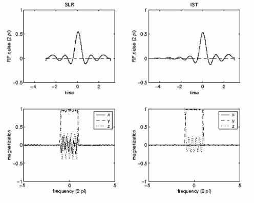
Figure 3.2.1. Comparison of SLR and IST equiripple pulses: $\rho=3$, $\delta_{2,\textrm{trans}}=0.01$, $\tau=0.2\times 2\pi$.

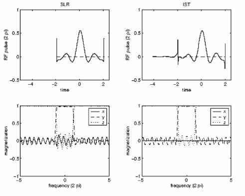
Figure 3.2.2. Comparison of SLR and IST equiripple pulses $\rho=2$, $\delta_{2,\textrm{trans}}=0.1$, $\tau=0.2\times 2\pi$.

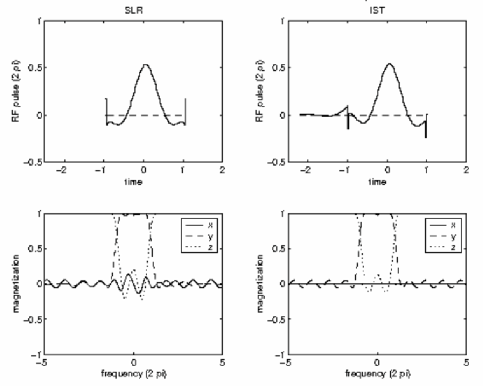
Figure 3.2.3. Comparison of SLR and IST equiripple pulses: $\rho=1$, $\delta_{2,\textrm{trans}}=0.05$, $\tau=0.5\times 2\pi$.

3.3. Self refocused pulse design

Suppose we want to design a pulse with zero rephasing time ($\rho=0$). Such a pulse is called a self refocused pulse. According to part (c) of Theorem 1.5.1, we should approximate the ideal reflection coefficient, $r_{\textrm{ideal}}$, by a function $r:\mathbb{R}\rightarrow\mathbb{C}$ which has a meromorphic extension to the upper half plane with $\lim_{|z|\rightarrow\infty}r(z)=0$. For example, $r$ could be a rational function with numerator degree strictly smaller than denominator degree. Of course, there are many ways to approximate $r_{\textrm{ideal}}$ in this way. The energy formula (1.7.1) tells us that the energy of the resulting pulse depends on the locations of the poles of $r$ in the upper half plane. If energy is a major concern, then $r$ should be designed to have a small number of poles, close to the real axis. In this way, there is a delicate trade-off between the energy of the pulse and the accuracy of the approximation. Another concern is the stability of the pulse under imperfect magnetic field conditions. For example, in many applications it is desirable for the pulse to maintain its selectivity when it is scaled by, say, 90% or 110%.

In this section we describe one method for designing relatively low energy, self refocused $90^{\circ}$ pulses. We need to approximate $r_{\textrm{ideal}}=\chi_{[-2,2]}$ by a function $r$ which has a meromorphic extension to the upper half plane. Let us write

$$r=\frac{e^{R}}{1+e^{R}},$$

where $R:\mathbb{R}\rightarrow\mathbb{C}$ has an analytic extension to the upper half plane. The idea is to choose $R$, so that $|e^{R}|$ is very large in-slice and very small out of slice. Then $r$ will be close to $r_{\textrm{ideal}}$. The magnitude of $e^{R}$ is determined by the real part of $R$, so we should design $\text{Re }R$ to be a smooth function of the form

$$\text{Re }R(\xi)=\begin{cases}k_{1}&\textrm{if }|\xi|<2\\ -k_{2}&\textrm{if }|\xi|>2+2\tau,\end{cases}$$

where $k_{1}$, $k_{2}$, and $\tau$ are positive numbers. The imaginary part of $R$ is then chosen so that $R$ has an analytic extension to the upper half plane. The parameters $k_{1}$ and $k_{2}$ control the in-slice and out-of-slice errors, respectively, and $\tau$ is the transition width. One can experiment with different values of these parameters to obtain a variety of pulses, with different energies. We plot one of these pulses in figure 3.3.1.

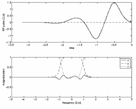
Figure 3.3.1. A self refocused pulse and its resulting magnetization.

Remark: Notice that the $r$ designed in the previous paragraph does not satisfy $\lim_{|\xi|\rightarrow\infty}r(\xi)=0$. This can be easily remedied by subtracting an appropriate, very small constant.

3.4. Half pulse design

In some applications it is only necessary to approximate the $x$-component of the ideal magnetization profile using a self refocused pulse. For example, see [11]. Let $\mathbf{M}_{\textrm{ideal},x}:\mathbb{R}\rightarrow\mathbb{R}$ be an ideal $x$-magnetization profile. We want to find a function $r$, which has a meromorphic extension to the upper half plane with $\lim_{|z|\rightarrow\infty}r(z)=0$ such that

$$\frac{2\text{Re }r}{1+|r|^{2}}\approx\mathbf{M}_{x}.$$

The trick is to set

$$r=\frac{1-R}{1+R},$$

where

$$R=\frac{1-r}{1+r}.$$

Then we have

$$\frac{2\text{Re }r}{1+|r|^{2}} = \frac{r+r^{*}}{1+r^{*}r}$$

$$= \frac{\frac{1-R}{1+R}+\frac{1-R^{*}}{1+R^{*}}}{1+\frac{1-R^{*}}{1+R^{*}}\frac{1-R}{1+R}}$$

$$= \frac{(1-R)(1+R^{*})+(1+R)(1-R^{*})}{(1+R)(1+R^{*})+(1-R)(1-R^{*})}$$

$$= \frac{1-|R|^{2}}{1+|R|^{2}}.$$

Therefore, we should design $R$ so that

$$|R|=\sqrt{\frac{1-\mathbf{M}_{x}}{1+\mathbf{M}_{x}}},$$

where $\mathbf{M}_{x}$ is a perhaps smoothed out version of $\mathbf{M}_{\textrm{ideal},x}$. The above calculations lead to the following

Proposition 3.4.1.

Let $\mathbf{M}_{x}:\mathbb{R}\rightarrow\mathbb{R}$ be an $x$-magnetization profile with sufficient smoothness and decay, and assume that $|\mathbf{M}_{x}(z)|<1$ for all $z\in\mathbb{R}$. Then there exist infinitely many self refocused pulses $\omega:\mathbb{R}\rightarrow\mathbb{C}$ such that $\mathcal{T}\omega=\mathbf{M}$. These pulses are parameterized by the poles of $\frac{1-r}{1+r}$ in the upper half plane, where $r$ is the reflection coefficient.

Remark 3.4.2.

The special case of no poles is often a minimum energy pulse. For example, this is the case whenever $\mathbf{M}_{x}$ is non-negative. Indeed then we have $|R|\leq 1$, which implies, by the maximum modulus principle, that $R$ is never equal to $-1$ in the upper half plane, which is equivalent to saying that $r=\frac{1-R}{1+R}$ has no poles in the upper half plane.

Figure 3.4.1 shows a pulse designed using this method.

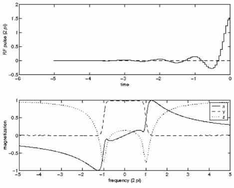
Figure 3.4.1. A half pulse and its resulting magnetization

Chapter 4 Conclusion

We have seen that the hard pulse approximation (the approximation of an RF-pulse by a sum of $\delta$-functions) leads to a discrete scattering theory which is completely analogous to the standard continuum scattering theory for the ZS-system. We introduced the DIST algorithm, a recursive algorithm for solving the full discrete inverse scattering problem relating to NMR pulse design, and we explained how this algorithm could be used to efficiently approximate the continuum inverse scattering transform. In the past, numerical techniques have been used to approximate the solutions to the Marchenko equations. In this thesis we have provided a more exact method of pulse design, which involves replacing the standard scattering data by, so called, discrete scattering data.

The case of pulses with finite rephasing time is particularly simple, and useful in practice. We described some new applications to NMR pulse design. Specifically we explained how to maintain control on the phase of the magnetization profile while producing equiripple pulses, self-refocused pulses, and half pulses.

Appendix A Notation and background material

A.0.1. Functions on the real line and the unit circle

In this thesis, we work with complex functions on the real line, $\mathbb{R}$, and the unit circle, $S^{1}$. If $f:\mathbb{R}\rightarrow\mathbb{C}$ is a function on the real line, then we say that $f$ has an analytic (meromorphic) extension to the upper half plane, $\mathbb{H}$, if there exists an analytic (meromorphic) function $\tilde{f}$ on $\mathbb{H}$ such that

$$\lim_{y\rightarrow 0^{+}}\tilde{f}(x+iy)=f(x)$$

for almost every $x\in\mathbb{R}$. Such an extension is necessarily unique. In this case we abuse notation and let $f$ also denote this extension $\tilde{f}$. Similarly, if $f:S^{1}\rightarrow\mathbb{C}$ is a function on the unit circle, then we say that $f$ has an analytic (meromorphic) extension to the unit disk, $\mathbb{D}$, if there exists an analytic (meromorphic) function $\tilde{f}$ on $\mathbb{D}$ such that the radial limits exist almost everywhere, and coincide almost everywhere with $f$. Again, we let $f$ denote both the function on $S^{1}$ and its extension to the unit disk.

When they are not being used to represent complex numbers, the symbols $\xi$ and $w$ will denote the identity functions on $\mathbb{R}$ and $S^{1}$, respectively. For example, if $r:\mathbb{R}\rightarrow\mathbb{C}$ is a function on the real line, then so is $\xi r$. Furthermore, if $r$ has a meromorphic extension to the upper half plane, then so does $\xi r$.

Let $\alpha^{*}$ denote the complex conjugate of the complex number $\alpha$. If $f$ is a function on the real line, we let $f^{*}$ denote the complex conjugate of $f$. If $f$ has an analytic (meromorphic) extension to the upper half plane, then we consider $f^{*}$ also as an analytic (meromorphic) function on the lower half plane given by

$$f^{*}(\xi)=f(\xi^{*})^{*}.$$

We follow similar conventions if $f$ is a function on $S^{1}$. Specifically, if $f$ has an analytic (meromorphic) extension to $\mathbb{D}$, then $f^{*}$ is considered as an analytic (meromorphic) function on $\hat{\mathbb{C}}\setminus\mathbb{D}$ given by

$$f^{*}(w)=f(\frac{1}{w^{*}})^{*}.$$

Here, $\hat{\mathbb{C}}$ is the Riemann sphere.

A.0.2. The Fourier transform

For $k>0$, we let $L^{k}(\mathbb{R})$ denote the space of equivalence classes of measurable functions $f:\mathbb{R}\rightarrow\mathbb{C}$ for which the quantity

$$\left\|f\right\|_{L^{k}}:=(\int_{-\infty}^{\infty}|f(z)|^{k}dz)^{\frac{1}{k}}$$

is finite. The functions $f$ and $g$ in $L^{k}(\mathbb{R})$ are considered to be equivalent if $\left\|f-g\right\|_{L^{k}}=0$. The space $L^{2}(\mathbb{R})$ is a Hilbert space with respect to the inner product

$$\left\langle f,g\right\rangle:=\int_{-\infty}^{\infty}f(z)g^{*}(z)dz.$$

We let $\mathcal{F}:L^{2}(\mathbb{R})\rightarrow L^{2}(\mathbb{R})$ denote the Fourier transform, and we write $\mathcal{F}(f)=\hat{f}$. For integrable $f$, the Fourier transform takes the form

$$\hat{f}(t)=\mathcal{F}(f)(t):=\int_{-\infty}^{\infty}f(z)e^{-itz}dz.$$

The Fourier transform is a unitary map, meaning it is a linear isomorphism which preserves the inner product, up to a factor of $2\pi$. We let $\mathcal{F}^{-1}$ denote the inverse of $\mathcal{F}$. For integrable $f$ we have

$$\check{f}(z)=\mathcal{F}^{-1}(f)(z)=\frac{1}{2\pi}\int_{-\infty}^{\infty}f(t)e^{itz}dt.$$

Similarly, we let $L^{k}(S^{1})$ denote the space of measurable functions $f:S^{1}\rightarrow\mathbb{C}$ for which the quantity

$$\left\|f\right\|_{L^{k}}:=(\frac{1}{2\pi}\int_{0}^{2\pi}|f(e^{i\theta})|^{k}d\theta)^{\frac{1}{k}}$$

is finite. The functions $f$ and $g$ in $L^{k}(S^{1})$ are considered to be equivalent if $\left\|f-g\right\|_{L^{k}}=0$. The space $L^{2}(S^{1})$ is a Hilbert space with respect to the inner product

$$\left\langle f,g\right\rangle:=\frac{1}{2\pi}\int_{0}^{2\pi}f(e^{i\theta})g^{*}(e^{i\theta})dz.$$

We let $\mathcal{F}:L^{2}(S^{1})\rightarrow\hat{L}^{2}(S^{1})$ denote the discrete Fourier transform, and we write $\mathcal{F}(f)=\hat{f}$. Here $\hat{L}^{2}(S^{1})$ is the Hilbert space of sequences $\hat{f}:\mathbb{Z}\rightarrow\mathbb{C}$ for which

$$\left\|\hat{f}\right\|_{\hat{L}^{2}}:=\sum_{j=-\infty}^{\infty}|\hat{f}(j)|^{2}$$

is finite. The inner product on $\hat{L}^{2}(S^{1})$ is given by

$$\left\langle\hat{f},\hat{g}\right\rangle:=\sum_{j=-\infty}^{\infty}\hat{f}(j)\hat{g}(j)^{*}.$$

Explicitly, we have

$$\hat{f}(j)=\mathcal{F}(f)(j):=\frac{1}{2\pi}\int_{0}^{2\pi}f(e^{i\theta})e^{-ij\theta}d\theta.$$

The discrete Fourier transform is a unitary map, meaning it is a linear isomorphism which preserves the inner product, up to a factor of $2\pi$. Again, we let $\mathcal{F}^{-1}$ denote its inverse. For absolutely summable sequences $S=\left\{a_{j}\right\}_{j\in\mathbb{Z}}$ we have

$$\mathcal{F}^{-1}(S)(e^{i\theta})=\sum_{j=-\infty}^{\infty}a_{j}e^{ij\theta}.$$

A.0.3. The Sobolev Space $H^{k}$

We say that $f:\mathbb{R}\rightarrow\mathbb{C}$ has a weak derivative $f^{\prime}:\mathbb{R}\rightarrow\mathbb{C}$ if for all smooth functions $\phi:\mathbb{R}\rightarrow\mathbb{C}$ with compact support we have

$$\int_{-\infty}^{\infty}f(x)\phi^{\prime}(x)dx+\int_{-\infty}^{\infty}f^{\prime}(x)\phi(x)dx=0.$$

The weak derivative of a function on $S^{1}$ is defined similarly.

Let $\Lambda=\mathbb{R}\textrm{ or }S^{1}$, and let $k$ be a non-negative integer. The Sobolev space $H^{k}(\Lambda)\subset L^{2}(\Lambda)$ consists of those functions which have $k$ weak derivatives in $L^{2}$. The spaces $H^{k}(\mathbb{R})$ and $H^{k}(S^{1})$ are Hilbert spaces with respect to the inner products

$$\left\langle f,g\right\rangle:=\sum_{j=0}^{k}\int_{-\infty}^{\infty}\partial^{j}f(x)\partial^{j}g^{*}(x)dx$$

and

$$\left\langle f,g\right\rangle:=\sum_{j=0}^{k}\frac{1}{2\pi}\int_{0}^{2\pi}\partial^{j}f(e^{i\theta})\partial^{j}g^{*}(e^{i\theta})d\theta,$$

respectively. Notice that $H^{0}(\Omega)=L^{2}(\Omega).$

These spaces are particularly simple in the Fourier domain. Let us define

$$\hat{H}^{k}(\mathbb{R}):=\left\{u\in L^{2}(\mathbb{R}):\;\int_{-\infty}^{\infty}(1+|x|)^{2k}|u(x)|^{2}dx<\infty\right\}$$

with the inner product

$$\left\langle u,v\right\rangle:=\frac{1}{2\pi}\int_{-\infty}^{\infty}(1+x^{2}+\dots+x^{2k})u(x)v^{*}(x)dx$$

and

$$\hat{H}^{k}(S^{1}):=\left\{u:\mathbb{Z}\rightarrow\mathbb{C}:\;\sum_{n=-\infty}^{\infty}(1+|n|)^{2k}|u(n)|^{2}<\infty\right\}$$

with the inner product

$$\left\langle u,v\right\rangle:=\sum_{n=-\infty}^{\infty}(1+n^{2}+\dots+n^{2k})u(n)v(n)^{*}.$$

Fact A.0.1.

Let $\Lambda=\mathbb{R}\textrm{ or }S^{1}$, and let $f$ be in $H^{1}(\Lambda)$. Then $\left\|f\right\|_{L^{\infty}}\leq\left\|f\right\|_{H^{1}}.$

Proof.

By the Cauchy-Schwartz inequality we have

$$|f(x)|^{2} = \left|2\int_{-\infty}^{x}f^{\prime}(y)f(y)dy\right|$$

$$\leq 2\int_{-\infty}^{x}|f^{\prime}(y)||f(y)|dy$$

$$\leq 2\left\langle f^{\prime},f\right\rangle$$

$$\leq 2\left\|f\right\|_{L^{2}}\left\|f^{\prime}\right\|_{L^{2}}$$

$$\leq \left\|f\right\|_{L^{2}}^{2}+\left\|f^{\prime}\right\|_{L^{2}}^{2}$$

$$= \left\|f\right\|_{H^{1}}^{2}.$$

∎

Fact A.0.2.

Let $\Lambda=\mathbb{R}\textrm{ or }S^{1}$. If $f$ and $g$ are in $H^{1}(\Lambda)$, then the product $fg$ is also in $H^{1}(\Lambda)$, and

$$\left\|fg\right\|_{H^{1}}\leq 2\left\|f\right\|_{H^{1}}\left\|g\right\|_{H^{1}}.$$

Proof.

We have

$$\left\|fg\right\|_{H^{1}}^{2} = \left\|fg\right\|_{L^{2}}^{2}+\left\|(fg)^{\prime}\right\|_{L^{2}}^{2}=\left\|fg\right\|_{L^{2}}^{2}+\left\|f^{\prime}g+fg^{\prime}\right\|_{L^{2}}^{2}$$

$$\leq \left\|f\right\|_{L^{\infty}}^{2}\left\|g\right\|_{L^{2}}^{2}+2\left\|f^{\prime}g\right\|_{L^{2}}^{2}+2\left\|fg^{\prime}\right\|_{L^{2}}^{2}$$

$$\leq \left\|f\right\|_{L^{\infty}}^{2}\left\|g\right\|_{L^{2}}^{2}+2\left\|f^{\prime}\right\|_{L^{2}}^{2}\left\|g\right\|_{L^{\infty}}^{2}+2\left\|f\right\|_{L^{\infty}}^{2}\left\|g^{\prime}\right\|_{L^{2}}^{2}$$

$$\leq 2\left\|f\right\|_{L^{\infty}}^{2}(\left\|g\right\|_{L^{2}}^{2}+\left\|g^{\prime}\right\|_{L^{2}}^{2})+2\left\|f^{\prime}\right\|_{L^{2}}^{2}\left\|g\right\|_{L^{\infty}}^{2}$$

$$\leq 4\left\|f\right\|_{H^{1}}^{2}\left\|g\right\|_{H^{1}}^{2}.$$

The last inequality uses Fact A.0.1. ∎

Fact A.0.3.

Let $\Lambda=\mathbb{R}\textrm{ or }S^{1}$. The Fourier transform is a unitary map from $H^{k}(\Lambda)$ onto $\hat{H}^{k}(\Lambda)$.

A.0.4. Self-adjoint operators

A bounded operator $A:H\rightarrow H$ on a complex Hilbert space is called self-adjoint if

$$\left\langle Av,w\right\rangle=\left\langle v,Aw\right\rangle\;\;\;\forall v,w\in H.$$

It is easy to verify that for such an operator $\left\langle Av,v\right\rangle$ is real for every $v\in H$. We say that $A$ is positive if

$$\left\langle Av,v\right\rangle>0$$

for all nonzero $v\in H$.

The following fact can be found in [8].

Fact A.0.4.

If $A:H\rightarrow H$ is a bounded, self-adjoint operator on a complex Hilbert space, then its operator norm is given by

$$\left\|A\right\|=\sup_{|v|=1}|\left\langle Av,v\right\rangle|.$$

The adjoint $A^{*}$ of a bounded operator $A:H\rightarrow H$ on a complex Hilbert space is defined by

$$\left\langle Av,w\right\rangle=\left\langle v,A^{*}w\right\rangle\;\;\;\forall v,w\in H.$$

The following two facts are easy to verify.

Fact A.0.5.

If $A$ and $A^{*}$ are bounded operators on a complex Hilbert space, then the operator $A^{*}A$ is self-adjoint and positive.

 

Fact A.0.6.

Let $A:X\rightarrow X$ be an operator on a Banach space. If $\left\|A\right\|=\alpha<1$, then $1+A$ is invertible.

 

Lemma A.0.7.

Suppose that $A:H\rightarrow H$ is bounded, self-adjoint and positive. Then

$$\left\|A-\frac{\gamma}{2}\right\|\leq\frac{\gamma}{2},$$

whenever $\gamma\geq\left\|A\right\|$.

Proof.

This follows from Fact A.0.4 and the estimate

$$\left|\left\langle v,(A-\frac{\gamma}{2})v\right\rangle\right|=\left|\left\langle v,Av\right\rangle-\frac{\gamma}{2}\left\langle v,v\right\rangle\right|\leq\frac{\gamma}{2}\left\langle v,v\right\rangle,$$

which holds since

$$0\leq\left\langle v,Av\right\rangle\leq\left\|A\right\|\left\langle v,v\right\rangle\leq\gamma\left\langle v,v\right\rangle.$$

∎

Proposition A.0.8.

Suppose that $A:H\rightarrow H$ is a bounded, positive self-adjoint operator on a complex Hilbert space. Then $1+A$ is invertible, and

$$\left\|(1+A)^{-1}\right\|\leq 1.$$

Proof.

The following method was used by Epstein in [5]. The trick is to set $\gamma=\left\|A\right\|$ and write

$$1+A=\frac{2+\gamma}{2}(1+B),$$

where

$$B=\frac{2}{2+\gamma}(A-\frac{\gamma}{2}).$$

Lemma A.0.7 tells us that

$$\left\|B\right\|\leq\frac{2}{2+\gamma}\cdot\frac{\gamma}{2}=\frac{\gamma}{2+\gamma}<1,$$

and so $1+B$ is invertible. Clearly, $1+A$ is also invertible.

Given $v\in H$, we know that

$$|(1+B)v|\geq(1-\frac{\gamma}{2+\gamma})|v|,$$

and hence

$$|(1+A)v| = \frac{2+\gamma}{2}|(1+B)v|$$

$$\geq \frac{2+\gamma}{2}(1-\frac{\gamma}{2+\gamma})|v|$$

$$= |v|,$$

which proves that

$$\left\|(1+A)^{-1}\right\|\leq 1.$$

∎

Appendix B The error from softening a pulse

As mentioned in the introduction, it is necessary, in practice, to replace a given hard pulse

$$\Omega_{\textrm{hard}}(t)=\sum_{j=-\infty}^{\infty}\omega_{j}\delta(t-j\Delta)$$

by a softened version

$$\Omega_{\textrm{soft}}(t)=\sum_{j=-\infty}^{\infty}\frac{\omega_{j}}{\Delta}\chi_{[0,\Delta)}(t-j\Delta).$$

In this section we estimate the difference between the magnetization profiles $\mathbf{M}_{\textrm{hard}}$ and $\mathbf{M}_{\textrm{soft}}$ resulting from $\Omega_{\textrm{hard}}$ and $\Omega_{\textrm{soft}}$, respectively.

Fix a frequency $z\in\mathbb{R}$. Let $M_{-,\textrm{hard}}(z;\Delta j)$ and $M_{-,\textrm{soft}}(z;\Delta j)$ denote the magnetizations at time $t=\Delta j$ (or the $j^{\textrm{th}}$ time step). These are normalized by

$$\lim_{j\rightarrow-\infty}M_{-,\textrm{hard}}(z;\Delta j)=\lim_{j\rightarrow-\infty}M_{-,\textrm{soft}}(z;\Delta j)=\left[\begin{array}[]{c}0\\ 0\\ 1\end{array}\right].$$

We are interested in the difference between $M_{-,\textrm{hard}}(z;j\Delta)$ and $M_{-,\textrm{soft}}(z;j\Delta)$ for large $j$.

Let us focus on the error introduced at the $j^{\textrm{th}}$ time step. Without loss of generality, we can assume that $\omega_{j}$ is real and positive. For the hard pulse, $M_{-,\textrm{hard}}(z;j+1)$ is obtained from $M_{-,\textrm{hard}}(z;j)$ by a rotation of $\omega_{j}$ radians around the $y$-axis, followed by a rotation of $\Delta z$ radians around the $z$-axis. On the other hand, one can check that $M_{-,\textrm{soft}}(z;j+1)$ is obtained from $M_{-,\textrm{soft}}(z;j)$ by a single rotation of $\gamma=\sqrt{\omega_{j}^{2}+(\Delta z)^{2}}$ radians around the $\left[\begin{array}[]{c}0\\ \omega_{j}/\gamma\\ \Delta z/\gamma\end{array}\right]$-axis. The difference between these rotations is a rotation of the sphere (around some axis) of some number $\theta_{j}$ of radians. If we can estimate $\theta_{j}$, then we can estimate the maximum spherical error introduced at the $j^{\textrm{th}}$ time step.

Let $R_{y}$ be rotation by $\omega_{j}$ radians around the $y$-axis, let $R_{z}$ be rotation by $\Delta z$ radians around the $z$-axis, and let $R_{yz}$ be rotation by $\gamma$ radians around the $\left[\begin{array}[]{c}0\\ \omega_{j}/\gamma\\ \Delta z/\gamma\end{array}\right]$-axis, where

$$\gamma=\sqrt{\omega_{j}^{2}+(\Delta z)^{2}}.$$

The question is: How well does $R_{yz}$ approximate $R_{z}R_{y}$?

These rotations are represented in $SU_{2}$ by

$$R_{y} = \left[\begin{array}[]{cc}\cos\frac{\omega_{j}}{2}&\sin\frac{\omega_{j}}{2}\\ -\sin\frac{\omega_{j}}{2}&\cos\frac{\omega_{j}}{2}\end{array}\right]$$

$$R_{z} = \left[\begin{array}[]{cc}\cos\frac{\Delta z}{2}+i\sin\frac{\Delta z}{2}&0\\ 0&\cos\frac{\Delta z}{2}-i\sin\frac{\Delta z}{2}\end{array}\right]$$

$$R_{yz} = \left[\begin{array}[]{cc}\cos\frac{\gamma}{2}+\frac{\Delta z}{\gamma}i\sin\frac{\gamma}{2}&\frac{\omega_{j}}{\gamma}\sin\frac{\gamma}{2}\\ -\frac{\omega_{j}}{\gamma}\sin\frac{\gamma}{2}&\cos\frac{\gamma}{2}-\frac{\Delta z}{\gamma}i\sin\frac{\gamma}{2}\end{array}\right].$$

Using a symbolic mathematics computer program, we compute the real part of the upper left component of the matrix $R_{yz}^{-1}R_{z}R_{y}\in SU_{2}$ to be

$$\phi(\omega_{j},\Delta z): = \cos(\frac{\omega_{j}}{2})\cos(\frac{\Delta z}{2})\cos(\frac{\gamma}{2})+\frac{\omega_{j}}{\gamma}\sin(\frac{\omega_{j}}{2})\cos(\frac{\Delta z}{2})\sin(\frac{\gamma}{2})$$

$$+\frac{\Delta z}{\gamma}\cos(\frac{\omega_{j}}{2})\sin(\frac{\Delta z}{2})\sin(\frac{\gamma}{2}),$$

which implies that $R_{yz}^{-1}R_{z}R_{y}$ is a rotation of $2\cos^{-1}\phi(\omega_{j},\Delta z)$ radians around some axis. From the Taylor expansion

$$\left(\cos^{-1}\phi(\alpha,\beta)\right)^{2}=\frac{1}{16}\omega_{j}^{2}(\Delta z)^{2}-\frac{1}{288}\omega_{j}^{4}(\Delta z)^{2}-\frac{1}{288}\omega_{j}^{2}(\Delta z)^{4}+\dots,$$

we see that, for reasonably small $\omega_{j}$ and $\Delta z$, $R_{yz}$ is extremely close to $R_{z}R_{y}$ composed with a rotation of $\frac{\Delta}{2}|\omega_{j}z|$ radians. In fact, numerical evidence suggests that $2\cos^{-1}\phi(\omega_{j},\Delta z)\leq\frac{\Delta}{2}|\omega_{j}z|$ for all $\omega$ and $\Delta z$.

Remark B.0.1.

The above conclusion would be the same if we replaced the axis of rotation of $R_{y}$ by some other axis orthogonal to the $z$-axis.

Applying the above result, the maximum error between $\mathbf{M}_{\textrm{hard}}(z)$ and $\mathbf{M}_{\textrm{soft}}(z)$ introduced at the $j^{th}$ step is conjectured to be a rotation of at most $\frac{\Delta}{2}|\omega_{j}z|$ radians, which would indicate a total error of at most

$$E=\frac{\Delta|z|}{2}\sum_{j=-\infty}^{\infty}|\omega_{j}|=\frac{\Delta|z|}{2}\int_{-\infty}^{\infty}|\Omega_{\textrm{soft}}(t)|dt$$

radians on the sphere. Thus we see that by reducing the time step, $\Delta$, the error introduced by softening a pulse can be made as small as we like over a fixed frequency interval.

Appendix C The case of non-simple zeros

In this section we consider the case where the poles of $a$ in the upper half plane (or unit disk) are not necessarily simple. We simply outline the idea, and leave most of the details to the interested reader.

In the case of simple zeros, the bound state data for the continuum scattering transform is encapsulated in the rational function

$$Q_{+,0}(\xi)=\sum_{k=1}^{m}\frac{C_{k}}{\xi-\xi_{k}}.$$

For each $t\in\mathbb{R}$, the rational functions

$$Q_{+,t}(\xi) = \sum_{k=1}^{m}\frac{C_{k}e^{2i\xi_{k}t}}{\xi-\xi_{k}}$$

$$Q_{-,t}(\xi) = \sum_{k=1}^{m}\frac{\tilde{C}_{k}e^{-2i\xi_{k}t}}{\xi-\xi_{k}}$$

can be uniquely determined from $Q_{+,0}$ using the following properties:

1. $Q_{+,t}$ has the form $Q_{+,t}(\xi)=\sum_{k=1}^{m}\frac{C_{k,t}}{\xi-\xi_{k}}$;

2. $Q_{-,t}$ has the form $Q_{-,t}(\xi)=\sum_{k=1}^{m}\frac{\tilde{C}_{k,t}}{\xi-\xi_{k}}$;

3. $Q_{+,t}=\Pi_{-}Q_{+,s}e^{2i\xi(t-s)}$ for all $t>s$;

4. $Q_{-,t}=\Pi_{-}Q_{-,s}e^{-2i\xi(t-s)}$ for all $t<s$;

5. The function $aQ_{-,t}Q_{+,t}+\frac{1}{a}$ is analytic in the upper half plane.

The fifth property can be verified by observing that the residue of $aQ_{-,t}Q_{+,t}+\frac{1}{a}$ at $\xi_{k}$ is

$$C_{k}\tilde{C}_{k}a^{\prime}(\xi_{k})+\frac{1}{a^{\prime}(\xi_{k})}=0.$$

Let us now handle the case where $a$ has non-simple zeros. Let $\xi_{1},\dots,\xi_{m}$ be complex numbers in the upper half plane, and let $d_{1},\dots,d_{m}$ be positive integers (representing the multiplicities). In this case, we specify the bound state data by defining the rational function

$$Q_{+,0}(\xi)=\sum_{k=1}^{m}\frac{P_{k}(\xi)}{(\xi-\xi_{k})^{d_{k}}},$$

where $P_{k}$ is a polynomial of degree $d_{k}-1$ which does not vanish at $\xi_{k}$. For each $t\in\mathbb{R}$, the rational functions $Q_{+,t}$ and $Q_{-,t}$ are defined by the following properties:

1. $Q_{+,t}$ has the form $Q_{+,t}(\xi)=\sum_{k=1}^{m}\frac{P_{k,t}(\xi)}{\xi-\xi_{k}}$, where $P_{k,t}$ is a polynomial of degree $k-1$;

2. $Q_{-,t}$ has the form $Q_{-,t}(\xi)=\sum_{k=1}^{m}\frac{\tilde{P}_{k,t}}{\xi-\xi_{k}},$where $\tilde{P}_{k,t}$ is a polynomial of degree $k-1$;

3. $Q_{+,t}=\Pi_{-}Q_{+,s}e^{2i\xi(t-s)}$ for all $t>s$;

4. $Q_{-,t}=\Pi_{-}Q_{-,s}e^{-2i\xi(t-s)}$ for all $t<s$;

5. The function $aQ_{-,t}Q_{+,t}+\frac{1}{a}$ is analytic in the upper half plane.

Once these functions have been determined, one can define the right and left Marchenko equations using

$$r_{t} = \Pi_{-}re^{2i\xi t}-Q_{+,t}$$

$$s_{t} = \Pi_{-}se^{-2i\xi t}-Q_{-,t}.$$

A similar method can be used in the discrete case.

Appendix D Explicit implementation of DIST

Let us write down some explicit formulas so that the DIST recursion can easily be implemented on a computer. We leave the derivations to the reader.

Given discrete scattering data

$$S=(a,b;w_{1},\dots,w_{m};c_{1}^{\prime},\dots,c_{m}^{\prime}),$$

we set

$$r = \frac{b}{a}$$

$$s = -\frac{b^{*}}{a}$$

and

$$c_{k} = \frac{c_{k}^{\prime}}{a^{\prime}(w_{k})}$$

$$\tilde{c}_{k} = -\frac{(c_{k}^{\prime})^{-1}w_{k}^{-1}}{a^{\prime}(w_{k})}.$$

• Step 1: Define the following sequences:

  $$f(n) = \hat{r}(n)-\sum_{k=1}^{m}c_{k}w_{k}^{-n}$$

  $$g(n) = \hat{s}(n)-\sum_{k=1}^{m}\tilde{c}_{k}w_{k}^{-n-1}.$$

• Step 2: Choose $M_{+}>>0$ and set

  $$\left[\begin{array}[]{c}K_{+,M_{+}}\\ L_{+,M_{+}}\end{array}\right]=\left[\begin{array}[]{c}1\\ 0\end{array}\right].$$

  Then define the polynomials $K_{+,j}$ and $L_{+,j}$ (for $j=0,1,\dots,M_{+}$) recursively using

  $$\left[\begin{array}[]{c}K_{+,j-1}\\ L_{+,j-1}\end{array}\right]=\left[\begin{array}[]{cc}1&-\gamma_{j}^{*}\\ \gamma_{j}w&w\end{array}\right]\left[\begin{array}[]{c}K_{+,j}\\ L_{+,j}\end{array}\right]$$

  and

  $$-\gamma_{j}^{*}=\frac{\sum_{n=0}^{\infty}f(-j-n)\hat{K}_{+,j}(n)}{\hat{K}_{+,j}(n)-\sum_{n=0}^{\infty}f(-j-n)\hat{L}_{+,j}(n)}.$$

• Step 3: Choose $M_{-}>>0$ and set

  $$\left[\begin{array}[]{c}K_{-,-M_{-}}\\ L_{-,-M_{-}}\end{array}\right]=\left[\begin{array}[]{c}1\\ 0\end{array}\right].$$

  Then define the polynomials $K_{-,j}$ and $L_{-,j}$ (for $j=-M_{-},\dots,-1,0$) recursively using

  $$\left[\begin{array}[]{c}K_{+,j+1}\\ L_{+,j+1}\end{array}\right]=\left[\begin{array}[]{cc}1&\gamma_{j}\\ -\gamma_{j}^{*}w&w\end{array}\right]\left[\begin{array}[]{c}K_{+,j}\\ L_{+,j}\end{array}\right]$$

  and

  $$\gamma_{j}=\frac{\sum_{n=0}^{\infty}g(j-n)\hat{K}_{-,j}(n)}{\hat{K}_{-,j}(n)-\sum_{n=0}^{\infty}g(j-n)\hat{L}_{-,j}(n)}.$$

• Step 4: Set

  $$\omega(t)=\sum_{j=-M_{-}}^{M_{+}}\omega_{j}\delta(t-j\Delta),$$

  where

  $$\omega_{j}=2i\frac{\gamma_{j}^{*}}{|\gamma_{j}|}\arctan|\gamma_{j}|.$$

Remark D.0.1.

If the left and right values of $\gamma_{0}$ are inconsistent, then $M_{+}$ and $M_{-}$ should be increased. Initially, these integers should be chosen so that

$$I_{+}=\sum_{n=M_{+}}^{\infty}|f(n)|$$

and

$$I_{-}=\sum_{n=M_{-}}^{\infty}|g(n)|$$

are small.

Appendix E Scattering on Lie groups

E.1. The scattering transform on Lie groups

The selective excitation transform fits into a more general framework. Let $G$ be a Lie group acting on a space $X$, with a special point $x_{0}\in X$. Fix an element $J\in\mathbf{g}$ in the Lie algebra of $G$ such that the one parameter subgroup $\left\{e^{Jz}:z\in\mathbb{R}\right\}\subset G$ is isomorphic to $S^{1}$. Also, fix a subspace $\mathbf{k}\subset\mathbf{g}$. Let $\omega:\mathbb{R}\rightarrow\mathbf{k}\subset\mathbf{g}$ be a function with sufficient smoothness and decay, so that there is a solution $v_{-}:\mathbb{R}\times\mathbb{R}\rightarrow X$ to the equation

(E.1.1) $$\partial_{t}v_{-}(z;t)=\left(\omega(t)+zJ\right)v_{-}(z;t)$$

normalized by

(E.1.2) $$\lim_{t\rightarrow-\infty}e^{-Jzt}v_{-}(z;t)=x_{0}.$$

For now, we assume that the solution $v_{-}$ is unique, and that

$$(\mathcal{T}_{G,J,\mathbf{k},X,x_{0}}\omega)(z):=\lim_{t\rightarrow\infty}e^{-Jzt}v_{-}(z;t)\in X$$

exists for all $z$. The operator $\mathcal{T}_{G,J,\mathbf{k},X,x_{0}}$ is called the scattering transform. It maps $\mathbf{k}$-valued functions of time into $X$-valued functions of frequency.

If we take $G=SO_{3}(\mathbb{R})$, $X=\mathbb{R}^{3}$, $x_{0}=\left[\begin{array}[]{c}0\\ 0\\ 1\end{array}\right]$, $J=\left[\begin{array}[]{ccc}0&1&0\\ -1&0&0\\ 0&0&0\end{array}\right]\in so_{3}(\mathbb{R})$, and

$$\mathbf{k}=\left\{\left[\begin{array}[]{ccc}0&0&-\text{Im }x\\ 0&0&\text{Re }x\\ \text{Im }x&-\text{Re }x&0\end{array}\right]:\;x\in\mathbb{C}\right\},$$

then $\mathcal{T}_{G,J,\mathbf{k},X,x_{0}}$ coincides with the selective excitation transform $\mathcal{T}$ defined above. For other examples of scattering transforms, see Section (E.3).

E.2. The scattering equation

Let us consider the scattering transform in the special case where $X=G$, $x_{0}=1\in G$, and $G$ acts on itself by left multiplication. To simplify notation we write

$$\mathcal{T}_{G,J,\mathbf{k}}:=\mathcal{T}_{G,J,\mathbf{k},G,1}.$$

This scattering transform is universal in the following sense:

Proposition E.2.1.

Let $G$, $J$, $\mathbf{k}$, $X$ and $x_{0}$ be as in Section E.1. Then

$$\mathcal{T}_{G,J,\mathbf{k},X,x_{0}}\omega=(\mathcal{T}_{G,J,\mathbf{k}}\omega)(x_{0}).$$

We omit the proof, which is a straightforward application of the definitions.

In this universal case, we consider two solutions $v_{\pm}:\mathbb{R}\times\mathbb{R}\rightarrow G$ to the equation

(E.2.1) $$\partial_{t}v_{\pm}(z;t)=\left(\omega(t)+zJ\right)v_{\pm}(z;t)$$

normalized by

(E.2.2) $$\lim_{t\rightarrow\pm\infty}e^{-Jzt}v_{\pm}(z;t)=1\in G.$$

The function

(E.2.3) $$S_{\omega}(z):=v_{+}(z;t)^{-1}v_{-}(z;t)$$

is independent of $t$ because given any two solutions $v_{1}$ and $v_{2}$ to equation (E.2.1) we have

$$\partial_{t}v_{1}^{-1}v_{2} = -v_{1}^{-1}(\partial_{t}v_{1})v_{1}^{-1}v_{2}+v_{1}^{-1}\partial_{t}v_{2}$$

$$= -v_{1}^{-1}\left(\omega(t)+zJ\right)v_{2}+v_{1}^{-1}\left(\omega(t)+zJ\right)v_{2}$$

$$= 0.$$

This calculation also demonstrates the uniqueness of $v_{-}$ and $v_{+}$. Letting $t$ tend to $\infty$, we find that

$$S_{\omega}(z)=\lim_{t\rightarrow\infty}e^{-Jzt}v_{-}(z;t)=(\mathcal{T}_{G,J,\mathbf{k}}\omega)(z)$$

so that $S_{\omega}$ is the scattering transformation $\mathcal{T}_{G,J,\mathbf{k}}$ applied to $\omega$. By Proposition E.2.1 we have

$$(\mathcal{T}_{G,J,\mathbf{k},X,x_{0}}\omega)(z)=S_{\omega}(z)\cdot x_{0}$$

whenever $G$ acts on a space $X$.

It is useful to define

$$u_{\pm}(z;t):=v_{\pm}(z;t)e^{-Jzt}.$$

In terms of this notation equations (E.2.1) through (E.2.3) become

(E.2.4) $$\partial_{t}u_{\pm}(z;t)=\omega(t)u_{\pm}(z;t)+z\left(Ju_{\pm}(z;t)-u_{\pm}(z;t)J\right)$$

(E.2.5) $$\lim_{t\rightarrow\pm\infty}u_{\pm}(z;t)=1\in G,$$

and

(E.2.6) $$S_{\omega}(z)=e^{-Jzt}v_{+}(z;t)^{-1}u_{-}(z;t)e^{Jzt}.$$

Equation (E.2.6) corresponds to the scattering equation (2.3.6).

E.3. Three scattering transforms

Let us fix $X=\hat{\mathbb{C}}$ to be the Riemann Sphere with $x_{0}=0$ and let $e^{J\mathbb{R}}\cong S^{1}$ be the group of rotations around the origin. There are three basic examples of scattering transforms (see Section E.1):

• Euclidean: $G=G_{E}=Aut(\mathbb{C})$ is the group of invertible affine transformations

  $$G_{E}=\left\{z\mapsto\lambda z+c:\;\lambda,c\in\mathbb{C},\;\lambda\neq 0\right\}.$$

• Spherical: $G=G_{S}\cong SO_{3}\mathbb{R}$ is the group of rigid rotations of the sphere.

• Hyperbolic: $G=G_{H}\cong PSL_{2}\mathbb{R}$ is the group of conformal automorphisms of the unit disk.

The second example corresponds to the selective excitation transform. Let us show that the first example (Euclidean) corresponds to the inverse Fourier transform.

We can represent

$$G_{E}=\left\{\left[\begin{array}[]{cc}\lambda&x\\ 0&1\end{array}\right]:\;\lambda\in\mathbb{C}^{*},x\in\mathbb{C}\right\}.$$

It is natural to choose $\mathbf{k}=\left[\begin{array}[]{cc}0&\mathbb{C}\\ 0&0\end{array}\right]$. Let us write

$$\omega(t)=\left[\begin{array}[]{cc}0&\omega(t)\\ 0&0\end{array}\right]$$

and

$$u_{-}(z;t)=\left[\begin{array}[]{cc}1&u_{-}(z;t)\\ 0&1\end{array}\right].$$

Then equation (E.2.4) is

$$\partial_{t}\left[\begin{array}[]{cc}1&u_{-}(z;t)\\ 0&1\end{array}\right]=\left[\begin{array}[]{cc}0&\omega(t)\\ 0&0\end{array}\right]\left[\begin{array}[]{cc}1&u_{-}(z;t)\\ 0&1\end{array}\right]+z\left[\begin{array}[]{cc}0&iu_{-}(z;t)\\ 0&0\end{array}\right]$$

or

$$\partial_{t}u_{-}(z;t)=\omega(t)+izu_{-}(z;t).$$

The solution normalized at $-\infty$ is

$$u_{-}(z;t)=\int_{-\infty}^{t}\omega(s)e^{i(t-s)z}ds,$$

and so

$$S_{\omega}(z)\cdot x_{0}=\int_{-\infty}^{\infty}\omega(s)e^{-isz}ds.$$

Therefore $T_{G,J,\mathbf{k},X,x_{0}}$ is the inverse Fourier transform.

E.4. The discrete scattering transform on Lie groups

Let $G$, $J$, $X$, and $x_{0}\in X$ be as in Section E.1. That is, $G$ is a Lie group acting on $X$, and $J\in\mathbf{g}$ is an element of the Lie algebra such that the one-parameter subgroup $e^{J\mathbb{R}}\subset G$ is isomorphic to $S^{1}$. This time we consider functions of the form $\Omega:\mathbb{Z}\rightarrow K\subset G$, where $K$ is some subset of $G$. Let us identify $S^{1}$ with the subgroup $e^{J\mathbb{R}}\subset G$, and set $\Omega_{j}=\Omega(j)$. Suppose there is a solution $V_{-}:S^{1}\times\mathbb{Z}\rightarrow X$ to the recursion

$$V_{-}(w;j+1)=w\Omega_{j}V_{-}(w;j)$$

normalized by

$$\lim_{j\rightarrow-\infty}w^{-j}V_{-}(w;j)=x_{0}.$$

Again, we assume that the solution is unique, and that

$$(\mathcal{T}_{G,J,K,X,x_{0}}^{\textrm{disc}}\Omega)(w):=\lim_{j\rightarrow+\infty}w^{-j}V_{-}(w;j)\in X$$

exists for every $w$. The transform $\mathcal{T}_{G,J,K,X,x_{0}}^{\textrm{disc}}$ is called the discrete scattering transform. It maps sequences in $K$ to loops in $X$.

If we take $G=SO_{3}(\mathbb{R})$, $X=\mathbb{R}^{3}$, $x_{0}=\left[\begin{array}[]{c}0\\ 0\\ 1\end{array}\right]$, $J=\left[\begin{array}[]{ccc}0&1&0\\ -1&0&0\\ 0&0&0\end{array}\right]\in so_{3}(\mathbb{R})$, and

$$K=\exp\left\{\left[\begin{array}[]{ccc}0&0&-\text{Im }x\\ 0&0&\text{Re }x\\ \text{Im }x&-\text{Re }x&0\end{array}\right]:\;x\in\mathbb{C}\right\},$$

then $\mathcal{T}_{G,J,K,X,x_{0}}^{\textrm{disc}}$ coincides with the discrete selective excitation transform $\mathcal{T}^{\textrm{disc}}$ defined above. Notice that $K$ consists of the rotations around axes orthogonal to the $z$-axis. For other examples of discrete scattering transforms, see Section (E.6).

E.5. The discrete scattering equation

Let us consider the discrete scattering transform in the special case where $X=G$, $x_{0}=1$ is the identity element, and $G$ acts on $X$ by left multiplication. To simplify notation we write

$$\mathcal{T}_{G,J,K}^{\textrm{disc}}:=\mathcal{T}_{G,J,K,G,1}^{\textrm{disc}}.$$

This discrete scattering transform is universal in the following sense:

Proposition E.5.1.

Let $G$, $J$, $K$, $X$ and $x_{0}$ be as in Section E.4. Then

$$\mathcal{T}_{G,J,K,X,x_{0}}^{\textrm{disc}}\Omega=(\mathcal{T}_{G,J,K}^{\textrm{disc}}\Omega)(x_{0}).$$

We omit the proof, which is a straightforward application of the definitions.

In this universal case, we consider two solutions $V_{\pm}:S^{1}\times\mathbb{Z}\rightarrow G$ to the recursion

(E.5.1) $$V_{\pm}(w;j+1)=w\Omega_{j}V_{\pm}(w;j)$$

normalized by

(E.5.2) $$\lim_{j\rightarrow\pm\infty}w^{-j}V_{\pm}(w;j)=1\in G.$$

The function

(E.5.3) $$S_{\Omega}^{\textrm{disc}}(w):=V_{+}(w;j)^{-1}V_{-}(w;j)$$

is independent of j because given any two solutions $V_{1}$ and $V_{2}$ to the recursion (E.5.1), we have

$$V_{1}(w;j+1)^{-1}V_{2}(w;j+1) = \left(V_{1}(w;j)^{-1}\Omega_{j}^{-1}w^{-1}\right)\left(w\Omega_{j}V_{2}(w;j)\right)$$

$$= V_{1}(w;j)^{-1}V_{2}(w;j).$$

This calculation, in particular, shows that $V_{-}$ and $V_{+}$ are unique. Letting $j$ tend to $\infty$, we find that

$$S_{\Omega}^{\textrm{disc}}(w)=\lim_{j\rightarrow\infty}w^{-j}V_{-}(w;j)=(\mathcal{T}_{G,J,\mathbf{k}}^{\textrm{disc}}\Omega)(w)$$

so that $S_{\Omega}^{\textrm{disc}}$ is the discrete scattering transformation $\mathcal{T}_{G,J,\mathbf{k}}^{\textrm{disc}}$ applied to $\Omega$.

It is useful to define

$$U_{\pm}(w;j):=V_{\pm}(w;j)w^{-j}.$$

In terms of this notation, equations (E.5.1) through (E.5.3) become

(E.5.4) $$U_{\pm}(w;j+1)=w\Omega_{j}U_{\pm}(w;j)w^{-1}$$

(E.5.5) $$\lim_{j\rightarrow\pm\infty}U_{\pm}(w;j)=1\in G,$$

and

(E.5.6) $$S_{\Omega}^{\textrm{disc}}(w)=w^{-j}U_{+}(w;j)^{-1}U_{-}(w;j)w^{j}.$$

Equation (E.5.6) corresponds to the scattering equation (2.4.7).

E.6. Three discrete scattering transforms

As in Section E.3 , we fix $X=\hat{\mathbb{C}}$ to be the Riemann Sphere with $x_{0}=0$ and let $e^{J\mathbb{R}}\cong S^{1}$ be the group of rotations around the origin. There are three basic examples of discrete scattering transforms (see Section E.4):

• Euclidean: $G=G_{E}=Aut(\mathbb{C})$ is the group of invertible affine transformations

  $$G_{E}=\left\{z\mapsto\lambda z+c:\;\lambda,c\in\mathbb{C},\;\lambda\neq 0\right\}.$$

• Spherical: $G=G_{S}\cong SO_{3}\mathbb{R}$ is the group of rigid rotations of the sphere.

• Hyperbolic: $G=G_{H}\cong PSL_{2}\mathbb{R}$ is the group of conformal automorphisms of the unit disk.

The second example corresponds to the discrete selective excitation transform. Let us show that the first example (Euclidean) corresponds to the discrete inverse Fourier transform.

We can represent

$$G_{E}=\left\{\left[\begin{array}[]{cc}\lambda&x\\ 0&1\end{array}\right]:\;\lambda\in\mathbb{C}^{*},x\in\mathbb{C}\right\}.$$

It is natural to choose $K=\left[\begin{array}[]{cc}1&\mathbb{C}\\ 0&1\end{array}\right]$. Let us write

$$\Omega_{j}=\left[\begin{array}[]{cc}1&\omega_{j}\\ 0&1\end{array}\right]$$

and

$$U_{-}(w;j)=\left[\begin{array}[]{cc}1&U_{-}(w;j)\\ 0&1\end{array}\right].$$

Then equation (E.5.4) is

$$\left[\begin{array}[]{cc}1&U_{-}(w;j+1)\\ 0&1\end{array}\right]=\left[\begin{array}[]{cc}w&0\\ 0&1\end{array}\right]\left[\begin{array}[]{cc}1&\omega_{j}\\ 0&1\end{array}\right]\left[\begin{array}[]{cc}1&U_{-}(w;j)\\ 0&1\end{array}\right]\left[\begin{array}[]{cc}w^{-1}&0\\ 0&1\end{array}\right]$$

or

$$U_{-}(w;j+1)=w(U_{-}(w;j)+\omega_{j}).$$

The solution normalized at $-\infty$ is

$$U_{-}(w;j)=\sum_{k=-\infty}^{j-1}\omega_{k}w^{(j-k)},$$

and so

$$(T_{G,J,K,X,x_{0}}^{\textrm{disc}}\Omega)(w)=S_{\omega}^{\textrm{disc}}(w)\cdot x_{0}=\sum_{k=-\infty}^{\infty}\omega_{k}w^{-k}.$$

Therefore $T_{G,J,K,X,x_{0}}^{\textrm{disc}}$ is the discrete inverse Fourier transform.

References

- [1] M. Ablowitz, D. Kaup, A. Newell, and H. Segur, The inverse scattering transform - Fourier analysis for nonlinear problems, Studies in Applied Math., 53 (1974), pp. 249-315.
- [2] M. Buonocore, RF Pulse Design Using the Inverse Scattering Transform, Magn. Reson. Med., 29 (1993), pp. 470-477.
- [3] J. Carlson, Exact solutions for selective-excitation pulses, Jour. of Mag. Res., 94 (1991), pp. 376-386.
- [4] C. L. Epstein, Introduction to Magnetic Resonance Imaging for Mathematicians, Ann. Inst. Fourier, 54(2004), pp. 185–210.
- [5] C. L. Epstein, Minimum energy pulse synthesis via the inverse scattering transform, Journal of Magnetic Resonance, 167 (2004), pp. 185-210.
- [6] L. Faddeev and L. Takhtajan, Hamiltonian Methods in the Theory of Solitons, Springer Verlag, Berlin, Heidelberg, New York, 1987.
- [7] P. Frangos and D. Jaggard, A Numerical solution to the Zakharov-Shabat inverse scattering problem, IEEE Transactions on Antennas and Propagation, 39 (1991), pp. 74-79.
- [8] P. Lax, Functional Analysis, John Wiley & Sons Inc., 2002.
- [9] P. Le Roux, Exact synthesis of radio frequency waveforms, Proceedings, 7th Annual Meeting for the Society of Magnetic Resonance Imaging in Medicine, 1988, p.1049.
- [10] J. Magland and C. Epstein, Practical pulse synthesis via the inverse scattering transform, Journal of Magnetic Resonance, 172(2005), pp. 63–78.
- [11] J. Magland and C. Epstein, Exact half pulse synthesis via the inverse scattering transform, Journal of Magnetic Resonance, 171/2(2004), pp. 305–131.
- [12] J. Pauly, P. Le Roux, D. Nishimura, and A. Macovski, Parameter relations for the Shinnar-Le Roux selective excitation pulse design algorithm, IEEE Trans. on Med. Imaging, 10 (1991), pp. 53-65.
- [13] L. Rabiner and B. Gold, Theory and application of digital signal processing, Prentice-Hall, Inc., Englewood Cliffs, NJ, 1975.
- [14] D. Rourke and P. Morris, The inverse scattering transform and its use in the exact inversion of the Bloch equation for noninteracting spins, Journal of Magnetic Resonance, 99 (1992), pp. 118-138.
- [15] M. Shinnar and J. Leigh, Inversion of the Bloch equation, J. Chem. Phys., 98 (1993), pp. 6121-6128.
- [16] A. E. Yagle, Inversion of the Bloch transform in magnetic resonance imaging using asymmetric two-component inverse scattering, Inverse Problems 6, (1990), pp. 133-151.