Dripping, pressure and surface tension of self-trapped laser beams

Abstract

We show that a laser beam which propagates through an optical medium with Kerr (focusing) and higher order (defocusing) nonlinearities displays pressure and surface-tension properties yielding capillarity and dripping effects totally analogous to usual liquid droplets. The system is reinterpreted in terms of a thermodynamic grand potential, allowing for the computation of the pressure and surface tension beyond the usual hydrodynamical approach based on Madelung transformation and the analogy with the Euler equation. We then show both analytically and numerically that the stationary soliton states of such a light system satisfy the Young-Laplace equation, and that the dynamical evolution through a capillary is described by the same law that governs the growth of droplets in an ordinary liquid system.

Introduction.- Since the pioneering paper of Piekara in the 70’spiekara74 , many works have highlighted the interesting properties of laser beams whose propagation is described by the so-called cubic-quintic (CQ) nonlinear Schrödinger equation (NLSE) with competing nonlinearities. Cavitation, superfluidity and coalescence have been investigatedjosserand1 ; josserand2 in the context of liquid He, where the model is a simple approach which does not take into account nonlocal interactions. Stable optical vortex solitons and the existence of top-flat states have also been reported in optical materials with CQ optical susceptibilityquiroga97 . Recent experiments about filamentation of high-power laser pulses have shown that the CQ regime could be achievable in $CS_{2}$ centurion05 as well in some chalcogenide glassessmektala00 . Recently, it has been also suggested that atomic coherence may be used to induce a giant CQ-like refractive index in Rb gas michinel06 .

On the other hand, this model has been shown to display surface properties in numerical simulations of soliton collisions edmundson95 , that have been considered as a trace of a liquid state of lightmichinel02 ; michinel06 . Here, we will provide the first analytical, quantitative demonstration of the liquid behavior of the system in ($2+1$) dimensions, both in its stationary soliton solutions and in the dynamical evolution when a light bump is forced to pass through a wave-guide simulating a capillary. In particular, we will provide the first consistent computation of the pressure and surface tension of the light bubbles in ($2+1$) dimensions, and show both analytically and numerically that they satisfy the Young-Laplace (Y-L) equation that gives the equilibrium of usual droplets. Subsequently, we will demonstrate that the system dripping properties are governed by the same generalized Y-L that applies to an ordinary liquid. These results show the deep connection between the nonlinear dynamics of laser beams and coherent liquids at zero temperature Chiao .

Thermodynamic model.- We will consider the paraxial propagation through an ideal CQ medium of a linearly polarized laser beam, being its complex amplitude distribution $\Psi$ described by a nonlinear Schrödinger equation of the adimensional form:

$$i\frac{\partial\Psi}{\partial z}+\frac{1}{2}\nabla_{\perp}^{2}\Psi+\gamma|\Psi|^{2}\Psi-\delta|\Psi|^{4}\Psi=0,$$ (1)

where $z$ is the propagation distance multiplied by $2\pi/\lambda$, being $\lambda$ the wavelength of the continuous light beam; $\nabla_{\perp}^{2}$ is the transverse Laplace operator in terms of $x,y$, the spatial variables multiplied by $2\pi\sqrt{2n_{0}}/\lambda$, being $n_{0}$ the linear refractive index of the medium; $\gamma$ and $\delta$ are proportional to the (opposite) $\chi^{(3)}$ and $\chi^{(5)}$ optical susceptibilities, respectively.

It is well-known that stationary version of Eq.(1) admits localized soliton-like solutions piekara74 of the form $\Psi_{A}(x,y,z)=A(x,y)e^{-i\mu z}$, being $\mu$ the propagation constant. In particular, it has been shown numerically that high power solitons feature top-flat profilesquiroga97 . These modes can only be calculated numerically and coexist with plane waves solutions of constant amplitude $\Psi_{A}(x,y,z)=Ae^{-i\mu z}$, which lead by substitution in Eq.(1) to $\mu=\delta|A|^{4}-\gamma|A|^{2}$. The existence domain for solitons is $\mu\in(\mu_{\infty},0)$, where $\mu_{\infty}=-\frac{3\gamma^{2}}{16\delta}$.

As discussed in physicaD , the stationary solutions of Eq. (1) can be derived from a variational principle $\frac{\delta\Omega}{\delta\psi^{*}}=0$ from the Landau’s grand potential $\Omega=H-\mu N$, where $H$ is the Hamiltonian, $N=\int|\Psi|^{2}d{\cal S}$ the particle number (in our system the photon flux through the transverse section ${\cal S}$) and $\mu$ the chemical potential which is thus identified in our case as the propagation constant we have defined above. The resulting expression is:

$$\Omega = \int\left[\frac{1}{2}|\nabla_{\perp}\Psi|^{2}-\frac{\gamma}{2}|\Psi|^{4}+\frac{\delta}{3}|\Psi|^{6}-\mu|\Psi|^{2}\right]d{\cal S},$$ (2)

In three dimensional systems, the partial derivative $\left(\partial\Omega/\partial{V}\right)_{\mu,T}$ of $\Omega$ with respect to the volume $V$ at constant chemical potential $\mu$ and temperature $T$ would give minus the pressure. Assuming a completely coherent two-dimensional model with $T=0K$, it is then natural to use the derivative of $\Omega$ with respect to the area $\cal S$, which yields:

$$p=-\left(\partial\Omega/\partial{\cal S}\right)_{\mu}=-\frac{1}{2}|\nabla_{\perp}\Psi|^{2}+\frac{\gamma}{2}|\Psi|^{4}-\frac{\delta}{3}|\Psi|^{6}+\mu|\Psi|^{2}.$$ (3)

Figure 1: [Color online] Plot of radius vs. propagation constant for different localized stationary solutions of Eq.(1). Solid (dashed) line corresponds to numerical (analytical) calculations. The left (right) inner picture, shows the field modulus profile (pressure distribution) of a stationary beam with $\mu/\mu_{\infty}=0.98$. Notice that close to the origin, the homogeneous pressure is positive whereas in the inhomogeneous region becomes negative.

In Fig.1 we plot an example of a ”flat-top” stationary state, corresponding to $\mu/\mu_{\infty}=0.98$, together with its pressure distribution. For all this type of solutions, in the wide flat region the value of the pressure is positive and equal to the central value $p(0)\equiv p_{c}$. Close to the origin it is straightforwardly obtained for the beam amplitude:

$$|A(0,0)|^{2}=\frac{\gamma}{2\delta}+\frac{\sqrt{\gamma^{2}+4\delta\mu}}{2\delta}$$ (4)

which yields for the pressure at the center of the beam ($p_{c}$) the following analytical expression:

$$p_{c}=\frac{(\gamma+\sqrt{\gamma^{2}+4\delta\mu})^{2}(-\gamma+2\sqrt{\gamma^{2}+4\delta\mu})}{24\delta^{2}}.$$ (5)

Notice that $p_{c}$ vanishes at the limits of the existence domain: $\mu=0$ (trivial zero-amplitude solution) and $\mu=\mu_{\infty}$ (infinite ”flat-top” with $|A_{\infty}|^{2}=0.75\gamma/\delta$). This result can be considered as a trace of the existence of two possible vacuum states in the systemphysicaD .

Limitations of the hydrodynamical analogy.- Our present purpose is to use the previous formalism in order to study the physical properties of the system. First, let us try to apply the commonly used hydrodynamical analogy, based on introducing the so-called Madelung TransformationMadelung $\psi=\rho^{1/2}e^{i\phi}$, where $\rho$ is a positive definite real function and $\phi$ is a real phase, eventually depending on the variables $x$, $y$ and $z$. After substituting in Eq.(1), and separating both the real and the imaginary part, we get two equations. The first one is a continuity equation, that is used to establish an analogy with hydrodynamics, and to argue that $\nabla\phi$ can be identified with a current, i.e. a velocity field ${\bf v}$. The second equation is

$$\frac{\partial{\bf v}}{\partial z}+\nabla_{\perp}\left(\frac{{\bf v}^{2}}{2}+\frac{1}{2\rho^{1/2}}\nabla_{\perp}^{2}\rho^{1/2}+\gamma\rho-\delta\rho^{2}\right)=0.$$ (6)

Here, the usual approachjosserand1 is to assume that the term $\frac{1}{2\rho^{1/2}}\nabla_{\perp}^{2}\rho^{1/2}$ can be neglected. In this case, Eq. (6) is identical to the known Euler equation of hydrodynamics provided that $\nabla_{\perp}(\gamma\rho-\delta\rho^{2})=-\frac{\nabla_{\perp}p}{\rho}$. This formula was used e.g. in Ref. josserand1 in order to derive an expression for the pressure of the homogenous phase, which coincides with our result of Eq. (5) for the top flat region of the solitons. One could hope that this analogy could be generalized also to the non-homogenous zones, such as that corresponding to values of the radial coordinate $r$ around the radius $R$ of the beam. However, we will see that this is not the case. For a (non-rotational) top flat soliton the phase term is simply equal to $\phi=-\mu z$, therefore ${\bf v}=\nabla_{\perp}\phi=0$. Note that $\mu$ is the propagation constant which is just a constant number for the given soliton. Therefore, by substituting in Eq. (6), we get

$$\nabla_{\perp}\left(\frac{1}{2\rho^{1/2}}\nabla_{\perp}^{2}\rho^{1/2}+\gamma\rho-\delta\rho^{2}\right)=0.$$ (7)

In other words, in this case the term that is usually neglected is exactly equal and opposite to the part that is used to compute the pressure. Therefore, neglecting such a term would correspond to a 100% error. In fact, for any soliton solution, having ${\bf v}=0$, Euler equation would unavoidably imply a constant pressure, which cannot be the case in any region where the spatial variation of the density is important. Nevertheless, in spite of this failure of the ordinary hydrodynamical approach, we will see that the ’pressure’ distribution in the non-homogeneous region can still be given a deep physical interpretation.

Equilibrium and surface tension.- Fig. 1 suggests that the $\Omega$ potential, as given by the spatial integral of minus the pressure, can be expressed as the sum of two contributions: one from the top-flat region, which is $-\pi R^{2}p_{c}$ with a good accuracy; and another from the region near the border, where the field is spatially-dependent, which is $-2\pi\int_{R}^{\infty}{rp(r)dr}$. Thus, we get the following analytical approximation for the $\Omega$ potential of the ”flat-top” solutions:

$$\Omega\simeq-\pi R^{2}p_{c}+2\pi\sigma R,$$ (8)

where we have defined a parameter $\sigma\equiv-\frac{1}{R}\int_{R}^{\infty}{rp(r)dr}$. We will now argue on how $\sigma$ can be identified with the surface tension of the light beam. In first place, we have computed numerically the parameter $\sigma$ for the different high-power top-flat solitons, and we have found that it converges quickly to a fixed value $\sigma\simeq 0.057$ as soon as $|\mu|$ approaches the limiting value $\mu_{\infty}$. In such a limit, the central pressure goes to zero and the only important contribution to the integral defining $\sigma$ comes from the gradient term of Eq. (3). Thus $\sigma\simeq-\frac{1}{2R}\int_{R}^{\infty}{r|\nabla_{\perp}\Psi|^{2}dr}$.

We can then get an analytical approximation for $\sigma$ by noting that for large $R$ and $r$, $\nabla_{\perp}\Psi\simeq d\Psi/dr$, and the multiplicating $r$ in the integrand can be approximated by $R$ in the comparatively thin ’surface’ region. Taking into account that for large $r$ Eq. (1) yields $A^{\prime}(r)^{2}\simeq-\gamma A(r)^{4}/2+\delta A(r)^{6}/3+\mu A(r)^{2}$, and by substituting the limiting value $\mu\to\mu_{\infty}=-\frac{3\gamma^{2}}{16\delta}$, we get after some algebra the expression:

$$\sigma\simeq\frac{9\gamma^{2}}{64\sqrt{6}\delta^{3/2}}.$$ (9)

For instance, the choice $\gamma=\delta=1$ gives $\sigma=0.057$, in complete agreement with our numerical value. By differentiating Eq. (8) and taking into account that $\sigma$ is constant, we get:

$$\frac{d\Omega}{dR}\simeq-\pi\left[\frac{d(R^{2}p_{c})}{dR}-2\sigma\right].$$ (10)

Our numerical calculations show that the growth in $R$ holds the thermodynamical equilibrium, (i.e.: $\frac{d\Omega}{dR}\simeq 0$), within a relative error which turns out to be as small as $\frac{d\Omega}{dR}<10^{-4}\frac{\Omega}{R}$ for all the range of ”flat-top” eigenmodes considered. Therefore, we can set $\frac{d\Omega}{dR}=0$ in Eq. (10), and we get $\frac{d(R^{2}p_{c})}{dR}=2\sigma$, or

$$p_{c}=2\frac{\sigma}{R},$$ (11)

which is the celebrated Young-Laplace (Y-L) equationLandau for spherical liquid droplets being $\sigma$ the surface tension of the system. Therefore, despite the failure of the usual hydrodynamic approach, we have demonstrated that the pressure distribution in the inhomogeneous region has a deep physical interpretation. In fact, the integral of the pressure in the non-homogeneous surface region gives the surface tension ($\sigma$), i.e. the inward force that compensates the outward positive inner force described by the pressure $p_{c}$, in order to keep the droplet stationary.

Figure 2: [Color online] Numerical simulation of the dripping behavior of light beams propagating through a channel waveguide highlighted with solid lines. As a comparison, the upper (lower) row corresponds to snapshots showing the evolution of the modulus of the quasi-gaussian (”flat-top”) solutions. The size of the pictures in x and y is the interval $[-250,250]$. The snapshots a)-d), b)-e), f) and c) correspond to propagation distances $z=0,11000,27000,45000$, respectively.

Instead of directly comparing Eq.(11) with the numerical simulation, we will equivalently test the inverted equation $R=2\sigma/p_{c}$, where $p_{c}$ can be expressed analytically in terms either of the central amplitude $A$ or of the propagation constant $\mu$, by using Eq. (5) and Eq.(9). This result provides the first analytical expression for the radius $R$ of the bidimensional top-flat solitons as a function e.g. of $\mu$, and is compared with the numerical solutions of the stationary version of Eq.(1) in Fig.1. As it can be appreciated in the figure, the agreement between the analytical formula and the numerical computation is remarkable, and becomes complete when $|\mu|$ approaches $|\mu_{\infty}|$. This result confirms our theoretical framework and provides the first formal demonstration, by validation of the Y-L equation, of the liquid properties of the ”flat-top” solutions in the ($2+1$) dimensional CQ model. Moreover, from Eq.(11) it can be inferred that, as $R\rightarrow\infty$, the value of $p_{c}$ vanishes, indicating that surface tension effects are not needed to balance the inner pressure, as it is the case of standard liquids described by the Y-L equation.

Dripping of light droplets.- In classical fluid mechanics, the presence of surface tension effects can be appreciated in the dynamical phenomenon of capillarity Landau ; surften_review . Here, in order to study droplets formation and dripping in our system, we have introduced in our mathematical model an external “channel-type” linear optical waveguide $V(x,y)$, superposed to the cubic-quintic nonlinearity. This waveguiding structure consists of three regions with indices $n_{1}=0.002$ $n_{2}=0.0028$ and $n_{3}=0.001$, which correspond to the top region($n_{1}$), central channel and bottom zones($n_{2}$) and rectangular regions flanking the central channel($n_{3}$), respectively, as it can be seen in the pictures of Fig.2. In our simulations, we compare the evolution of two initial eigenstate beams with propagation constants $\mu/\mu_{\infty}=0.01$ (quasi-gaussian beam of Fig.2a) and $\mu/\mu_{\infty}=0.98$ (”flat-top” beam of Fig.2d), both located within the waveguide top region. Depending on the channel size, and keeping $n_{3}<n_{2},n_{1}$, above a given value of $\Delta n=n_{2}-n_{1}$ in both cases a significant amount of beam power starts to flow from the initial eigenstate through the channel, as shown in (Figs.2b and 2e). It is noteworthy that the light stream inside the channel does not suffer any unstabilization and remains connected to the initial source of light, i.e., the guide prevents the appearance of modulational instability. At the output of the channel, it can be seen in Fig.2c that the low-power distribution spreads like a (coherent) gas in free expansion. However, the light flowing from the ”flat-top” beam yields to the formation of a droplet, as it can be appreciated in Fig.2f and in more detail in the insets of Fig.3.

As it can be seen in the insets of Fig.3, just before the release of the droplet the falling column of liquid light becomes narrower, just as in the well-known case of usual liquid streams falling from a tapdripping2 . On the other hand, all the steps in Fig.2 are qualitatively very similar to those obtained both in real experiments and in simulations with liquids surften_review -dripping1 .

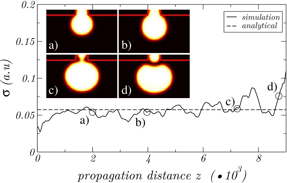
Figure 3: [Color online] Numerically calculated values of the surface tension along the droplet-formation process. Solid (dashed) line corresponds to numerical (analytical) calculations of $\sigma$. Insets: snapshots showing different stages of evolution of the light droplet for different values of $z$. Circles in the figure refer to upper insets. The spatial scales spanned are $x\in[-50,50],y\in[-20,-80]$.

Finally, we have also performed a quantitative test by comparing the numerical simulation with the generalized Y-L equation that describes the growth of an elliptic bubble of an ordinary liquid system, $p_{c}=\sigma(\frac{1}{R_{I}}+\frac{1}{R_{II}})$, where $R_{I}$ and $R_{II}$ are the principal radii Landau . In Fig.3, we have plotted the quantity $\sigma=p_{c}/(\frac{1}{R_{I}}+\frac{1}{R_{II}})$ for the “dripping” simulation of Fig.2 at several propagation distances, assuming $z=0$ where the light droplet first appears. We see that the numerical value of $\sigma$ oscillates around the same value that we have calculated analytically in Eq.(9) for the stationary solutions. This demonstrates that the droplets are formed close to stationary equilibrium, and they grow according to the generalized Y-L equation as in the case of an ordinary liquid.

Conclusions.-. We have provided the first consistent computation of the pressure and surface tension of the soliton solutions appearing in the propagation of self-trapped laser beams described by the ($2+1$) dimensional CQ-NLSE, and we have shown both analytically and numerically that they satisfy the Young-Laplace equation that governs the equilibrium of usual liquid droplets. Subsequently, we have also demonstrated that the system dripping properties are governed by the same generalized Y-L that applies to an ordinary liquid. These results reveal the deep connection between the physics of self-trapped laser beams and quantum liquids at zero temperature, opening the door for the quest of these new states of matter in the frame of current nonlinear optics experiments.

Acknowledgements.- We thank A. Ferrando for useful discussions. This work was supported by MEC, Spain (projects FIS2006-04190 and FIS2007-62560) and Xunta de Galicia (project PGIDIT04TIC383001PR and D.N. grant from Consellería de Innovación e Industria-Xunta de Galicia).

References

- (1) A. H. Piekara, J. S. Moore, and M. S. Feld, Phys. Rev. A9, 1403–1407 (1974).
- (2) C. Josserand, Y. Pomeau and S. Rica, Phys. Rev. Lett. 75, 3150–3153 (1995);
- (3) C. Josserand and Sergio Rica, Phys. Rev. Lett. 78, 1215–1218 (1997).
- (4) M. Quiroga-Teixeiro and H. Michinel, J. Opt. Soc. Am. B14, 2004–2009 (1997); D. Mihalache, et al., Phys. Rev. Lett. 88, 073902 (2002).
- (5) M. Centurion et al., Phys. Rev. A71, 063811 (2005).
- (6) F. Smektala, C. Quemard, V. Couderc, and A. Barthelemy, J. Non-Cryst. Sol., 274, 232–237 (2000).
- (7) H. Michinel, M. J. Paz-Alonso and V. M. Pérez García, Phys. Rev. Lett. 96, 023903 (2006); A. Alexandrescu, H. Michinel and V. M. Pérez-García, Phys. Rev. A79, 013833 (2009).
- (8) D. E. Edmundson and R. H. Enns, Phys. Rev. A51, 2491–2498 (1995); M. J. Paz-Alonso et al., Phys. Rev. E69 , 056601 (2004).
- (9) H. Michinel et al., Phys. Rev. E65, 066604 (2002).
- (10) R. Y. Chiao, Opt. Commun. 179, 157–166 (2000); R. Y. Chiao et al., J. Phys. B: At. Mol. Opt. Phys 37, S81–S89 (2004); R. Y. Chiao et al., Phys. Rev. A69, 063816 (2004).
- (11) D. Novoa et al., Physica D (2009), doi:10.1016/j.physd.2009.02.002.
- (12) E. Madelung, “Die Mathematischen Hilfsmittel des Physikers”, (Springer-Verlag, Berlin, 1957).
- (13) L. D. Landau and E. M. Lifshitz, “Fluid Mechanics”, (Pergamon, Oxford, 1984).
- (14) J. Eggers, Rev. Mod. Phys. 69, 3 (1997).
- (15) V. Grubelnik and M. Marhl, Am. J. Phys. 73, 5 (2005).
- (16) R. Suryo and O. A. Basaran, Phys. Rev. Lett. 96, 034504 (2006).
- (17) O. E. Yildirim, Q. Xu, and O. A. Basaran, Phys. Fluids 17, 062107 (2005).