Turing Instability for a Ratio-Dependent Predator-Prey Model with Diffusion

Abstract

Ratio-dependent predator-prey models have been increasingly favored by field ecologists where predator-prey interactions have to be taken into account the process of predation search. In this paper we study the conditions of the existence and stability properties of the equilibrium solutions in a reaction-diffusion model in which predator mortality is neither a constant nor an unbounded function, but it is increasing with the predator abundance. We show that analytically at a certain critical value a diffusion driven (Turing type) instability occurs, i.e. the stationary solution stays stable with respect to the kinetic system (the system without diffusion). We also show that the stationary solution becomes unstable with respect to the system with diffusion and that Turing bifurcation takes place: a spatially non-homogenous (non-constant) solution (structure or pattern) arises. A numerical scheme that preserve the positivity of the numerical solutions and the boundedness of prey solution will be presented. Numerical examples are also included.

1 Introduction

Since it is rare to find a pair of biological species in nature which meet precise prey-dependence or ratio-dependence functional responses in predator-prey models, especially when predators have to search for food (and therefore, have to share or compete for food), a more suitable general predator-prey theory should be based on the so-called ratio-dependent theory (see [1, 2, 3, 4]). The theory may be stated as follows: the per capita predator growth rate should be a function of the ratio of prey to predator abundance, and so should be the so-called predator functional response. Such cases are strongly supported by numerous field and laboratory experiments and observations (see, for instance, [5, 6, 7, 8]).

Denote by $N(t)$ and $P(t)$ the population densities of prey and predator at time $t,$ respectively. Then the ratio-dependent type predator-prey model with Michaelis-Menten type functional response is given as follows:

$$\frac{dN}{dt}&=rN\left(1-\frac{N}{K}\right)-\frac{aNP}{mP+N},\\ \frac{dP}{dt}=P\left[-Q(P)+\frac{bN}{mP+N}\right],$$ (1.1)

where $a,b,m,K,$ and $r$ are positive constants. In (1.1), $Q(P)$ denotes a mortality function of predator, and $r$ and $K$ the prey growth rate with intrinsic growth rate and carrying capacity in the absence of predation, respectively, while $a,b,$ and $m$ are model-dependent constants.

From a formal point of view, this model looks very similar to the well-known Michaelis-Menten-Holling predator-prey model:

$$\frac{dN}{dt}&=rN\left(1-\frac{N}{K}\right)-\frac{aNP}{c+N},\\ \frac{dP}{dt}=P\left[-Q(P)+\frac{bN}{c+N}\right].$$ (1.2)

Indeed, the only difference between Models (1.1) and (1.2) is that the parameter $c$ in (1.2) is replaced by $mP$ in (1.1). Both terms $mP$ and $c$ are proportional to the so-called searching time of the predator, namely, the time spent by each predator to find one prey. Thus, in the Michaelis-Menten-Holling model (1.2) the searching time is assumed to be independent of predator density, while in the ratio-dependent Michaelis-Menten type model (1.1) it is proportional to predator density (i.e., other predators strongly interfere).

Predators and preys are usually abundant in space with different densities at difference positions and they are diffusive. Several papers have focused on the effect of diffusion which plays a crucial role in permanence and stability of population (see [9, 10, 11, 12, 13, 14, 15], and the references therein). Especially in [13] the effect of variable dispersion rates on Turing instability was extensively studied, and in [11] the dynamics of ratio-dependent system has been analyzed in details with diffusion and delay terms included. Cavani and Farkas (see [16]) have considered a modification of (1.2) when a diffusion was introduced, yielding:

$$\frac{\partial N}{\partial t}&=rN\left(1-\frac{N}{K}\right)-\frac{aNP}{c+N}+D_{1}\frac{\partial^{2}N}{\partial x^{2}},\quad x\in(0,l),t>0,\\ \frac{\partial P}{\partial t}=P\left[-Q(P)+\frac{bN}{c+N}\right]+D_{2}\frac{\partial^{2}P}{\partial x^{2}},\quad x\in(0,l),t>0,$$ (1.3)

where the specific mortality of the predator is given by

$$Q(P)=\frac{\gamma+\delta P}{1+P},$$ (1.4)

which depends on the quantity of predator. Here, the positive constants $\gamma$ and $\delta$ denote the minimal mortality and the limiting mortality of the predator, respectively. Throughout the paper, the following natural condition

$$0<\gamma\leq\delta$$ (1.5)

will be assumed, and we will consider the case of the constant diffusivity, $D_{i}>0$, $i=1,2$. The advantage of this model is that the predator mortality is neither a constant nor an unbounded function, but still it is increasing with the predator abundance. On the other hand, combining (1.1) and (1.3), many authors (see [17, 15, 18], for instance) have studied a more general model as follows:

$$\frac{\partial N}{\partial t}&=rN\left(1-\frac{N}{K}\right)-\frac{aNP}{mP+N}+D_{1}\frac{\partial^{2}N}{\partial x^{2}},\quad x\in(0,l),t>0,\\ \frac{\partial P}{\partial t}=P\left[-Q(P)+\frac{bN}{mP+N}\right]+D_{2}\frac{\partial^{2}P}{\partial x^{2}},\quad x\in(0,l),t>0,$$ (1.6)

with the specific mortality of the predator somewhat restricted in the form

$$Q(P)=d.$$ (1.7)

In this paper we consider a ratio-dependent reaction-diffusion predator-prey model with Michaelis-Menten type functional response and the specific mortality of the predator given by (1.4) instead of (1.7). We study the effect of the diffusion on the stability of the stationary solutions. Also we explore under which parameter values Turing instability can occur giving rise to non-uniform stationary solutions satisfying the following equations:

$$\frac{\partial N}{\partial t}&=rN\left(1-\frac{N}{K}\right)-\frac{aNP}{mP+N}+D_{1}\frac{\partial^{2}N}{\partial x^{2}},\quad x\in(0,l),t>0,\\ \frac{\partial P}{\partial t}=P\left[-\frac{\gamma+\delta P}{1+P}+\frac{bN}{mP+N}\right]+D_{2}\frac{\partial^{2}P}{\partial x^{2}},\quad x\in(0,l),t>0,$$ (1.8)

assuming that prey and predator are diffusing according to Fick’s law in the interval $x\in[0,l].$ We are interested in the solutions $N,P:(l,0)\times\mathbb{R}^{+}\rightarrow\mathbb{R}^{+}$ fulfilling the Neumann boundary conditions

$$N_{x}(0,t)=N_{x}(l,t)=P_{x}(0,t)=P_{x}(l,t)=0,$$ (1.9)

and initial conditions

$$N(x,0)\geq 0,\quad P(x,0)\geq 0,\quad x\in(0,l).$$

For simplicity, we nondimensionalize the system (1.8) with the following scaling

$$\widetilde{t}=rt,\quad\widetilde{N}=\frac{N}{K},\quad\widetilde{P}=\frac{mP}{K},$$

and letting

$$\alpha=\dfrac{a}{mr},\;\widetilde{\gamma}=\dfrac{\gamma}{b},\;\widetilde{\delta}=\dfrac{\delta}{b},\;\epsilon=\dfrac{b}{r},\;\beta=\frac{K}{m},\;d_{1}=\dfrac{D_{1}}{r},\;d_{2}=\dfrac{D_{2}}{r}.$$

For the sake of simplification of notations, dropping tildes, the system (1.8) takes the form

$$\frac{\partial N}{\partial t}&=N(1-N)-\frac{\alpha NP}{P+N}+d_{1}\frac{\partial^{2}N}{\partial x^{2}},\quad x\in(0,l),t>0,\\ \frac{\partial P}{\partial t}=\epsilon P\left[-\frac{\gamma+\delta\beta P}{1+\beta P}+\frac{N}{P+N}\right]+d_{2}\frac{\partial^{2}P}{\partial x^{2}},\quad x\in(0,l),t>0.$$ (1.10)

Set

$$\mathbf{F}=\left(\begin{array}[]{c}F_{1}\\ F_{2}\end{array}\right),\mathbf{u}:=\left(\begin{array}[]{c}N\\ P\end{array}\right)D:=\left(\begin{array}[]{cc}d_{1}&0\\ 0&d_{2}\end{array}\right),$$

where

$$F_{1}(N,P)=N(1-N)-\frac{\alpha NP}{P+N},\quad F_{2}(N,P)=\epsilon P\left[-\frac{\gamma+\delta\beta P}{1+\beta P}+\frac{N}{P+N}\right].$$

Then the system (1.10) with the boundary conditions (1.9) takes the form

$$\mathbf{u}_{t}=\mathbf{F}(\mathbf{u})+D\frac{\partial^{2}\mathbf{u}}{\partial x^{2}};\quad\mathbf{u}_{x}(0,t)=\mathbf{u}_{x}(l,t)=\mathbf{0}.$$ (1.11)

Clearly, in case the predator and prey are spatially homogeneous, the spatially constant solution $\mathbf{u}(t)=(N(t),P(t))^{T}$ of (1.11), fulfilling the boundary conditions obviously, satisfies the kinetic system

$$\mathbf{u}_{t}=\mathbf{F}(\mathbf{u}).$$ (1.12)

2 The model without diffusion

In this section we will study the system (1.10) without diffusion, i.e.,

$$\frac{dN}{dt}&=N(1-N)-\frac{\alpha NP}{P+N},\\ \frac{dP}{dt}=\epsilon P\left[-\frac{\gamma+\delta\beta P}{1+\beta P}+\frac{N}{P+N}\right].$$ (2.1)

In particular, we will focus on the existence of equilibria and their local stability. This information will be crucial in the next section where we study the effect of the diffusion parameters on the stability of the steady states.

The equilibria of the system (2.1) are given by the solution of the following equations

$$N(1-N)-\frac{\alpha NP}{P+N}=0,\quad\epsilon P\left(-\frac{\gamma+\delta\beta P}{1+\beta P}+\frac{N}{P+N}\right)=0.$$

The system has at least one equilibrium with positive values. This is the point of intersection of the prey null-cline

$$P=H_{1}(N)=\frac{(1-N)N}{\alpha-(1-N)}$$

and the predator null-cline

$$P=H_{2}(N)=\frac{\gamma-\beta(1-\delta)N+2\sqrt{\left\{\gamma-\beta(1-\delta)N\right\}^{2}-4\beta\delta(1-\gamma)N}}{2\beta\delta}.$$

Thus, denoting the coordinates of a positive equilibrium by $(\overline{N},\overline{P})$, these coordinates satisfy $\overline{P}=H_{1}(\overline{N})=H_{2}(\overline{N}).$

The Jacobian matrix of the system (2.1) linearized at $(\overline{N},\overline{P})$ is

$$A=\left(\begin{array}[]{lr}\Theta_{1}&-\Theta_{2}\\ \Theta_{3}&-\Theta_{4}\end{array}\right),$$ (2.2)

where

$$\operatorname{trace}A=\Theta_{1}-\Theta_{4},\operatorname{det}A=\Theta_{2}\Theta_{3}-\Theta_{1}\Theta_{4}$$

and

$$\Theta_{1}&=-\overline{N}+\frac{\alpha\overline{N}\,\overline{P}}{(\overline{P}+\overline{N})^{2}},\quad\Theta_{2}=\frac{\alpha\overline{N}^{2}}{(\overline{P}+\overline{N})^{2}},\\ \Theta_{3}=\frac{\epsilon\overline{P}^{2}}{(\overline{P}+\overline{N})^{2}},\quad\Theta_{4}=\frac{\epsilon\beta\overline{P}(\delta-\gamma)}{(1+\beta\overline{P})^{2}}+\frac{\epsilon\overline{N}\,\overline{P}}{(\overline{P}+\overline{N})^{2}}.$$ (2.3)

The characteristic equation is given by

$$\lambda^{2}-\left(\operatorname{trace}A\right)\lambda+\operatorname{det}A=0.$$

Recall that $(\overline{N},\overline{P})$ is locally asymptotically stable if $\operatorname{Re}\lambda<0$, which is equivalent to have $\operatorname{trace}A<0$ and $\operatorname{det}A>0$. For this, we will assume that

$$\Theta_{1}<\Theta_{4},\quad\Theta_{2}\Theta_{3}>\Theta_{1}\Theta_{4}.$$ (2.4)

Remark 2.1.

Due to (1.5), we see that $\Theta_{4}>0$. If $\Theta_{1}\leq 0$, then the two conditions in (2.4) hold.

3 The model with diffusion

In this section we will investigate in Turing instability and bifurcation for our model problem. We will also study pattern formation of the predator-prey solutions.

3.1 Local existence of solutions

Before studying the stability of equilibrium solutions, we will discuss about the local existence and uniqueness of solution for a given ratio-dependent reaction-diffusion predator-prey model. Applying the criteria for the local existence of solution (see [19, 20]) to the nonlinear parabolic systems (1.11), we see that there exists a unique local solution of the given system.

Let $\Omega$ be a bounded region in $\mathbb{R}^{n},n\geq 2,$ with smooth boundary $\partial\Omega$ and $\nu$ denotes the unit outward normal to $\Omega$. Then Morgan considered in reference ([19]) essentially of the form

$$\mathbf{u}_{t}(x,t)&=D\Delta\mathbf{u}(x,t)+f(\mathbf{u}(x,t)),\quad x\in\Omega,t>0,\\ \frac{\partial\mathbf{u}(x,t)}{\partial\nu}=\mathbf{0},\quad x\in\partial\Omega,t>0,\\ \mathbf{u}(x,0)=\mathbf{u}_{0}(x),\quad x\in\Omega,$$ (3.1)

where $\mathbf{u}:\Omega\times(0,\infty)\rightarrow\mathbb{R}^{m},$ $f:\mathbb{R}^{m}\rightarrow\mathbb{R}^{m}$ is a locally Lipschitz continuous function, $D$ is an $m\times m$ diagonal matrix with diagonal entries $d_{j}>0$, and $\mathbf{u}_{0}:\Omega\rightarrow\mathbb{R}^{m}$ is bounded and measurable. Then the following theorem holds [19]:

Theorem 3.1.

Under the assumptions on (3.1) stated above, there exists $T_{\operatorname{max}}>0$ and $M=(M_{j})\in C([0,T_{\operatorname{max}}),\mathbb{R}^{m})$ such that
(i) (3.1) has a unique classical solution $\mathbf{u}$ on $\overline{\Omega}\times[0,T_{\operatorname{max}})$ which cannot be continued to $[0,T)$ for any $T>T_{\operatorname{max}}$, and
(ii) $|\mathbf{u}_{j}(\cdot,t)|_{\infty,\Omega}\leq M_{j}(t)$ for all $1\leq j\leq m,0\leq t<T_{\operatorname{max}}$.
Moreover, if $T_{\operatorname{max}}<\infty$, then $|\mathbf{u}_{j}(\cdot,t)|_{\infty,\Omega}\rightarrow\infty$ as $t\rightarrow T_{\operatorname{max}^{-}}$ for some $1\leq j\leq m$.

Defining $F_{1}(0,0)=0$ and $F_{2}(0,0)=0$ in our model (1.11), Theorem 3.1 implies local existence and uniqueness. More precisely, there exists $T_{\operatorname{max}}>0$ and $N_{M}$ and $P_{M}\in C([0,T_{\operatorname{max}}))$ such that
(i) (3.1) has a unique classical solution $\mathbf{u}=(N,P)^{T}$ on $[0,l]\times[0,T_{\operatorname{max}})$ which cannot be continued to $[0,T)$ for any $T>T_{\operatorname{max}}$, and
(ii) $|N(\cdot,t)|_{\infty,(0,l)}\leq N_{M}(t)$ and $|P(\cdot,t)|_{\infty,(0,l)}\leq P_{M}(t)$ for $0\leq t<T_{\operatorname{max}}$.
Moreover, if $T_{\operatorname{max}}<\infty$, then either $|N(\cdot,t)|_{\infty,(0,l)}\rightarrow\infty$ or $|P(\cdot,t)|_{\infty,(0,l)}\rightarrow\infty$ as $t\rightarrow T_{\operatorname{max}^{-}}.$

3.2 Turing instability

Definition 3.2.

We say that the equilibrium $(\overline{N},\overline{P})$ is Turing unstable if it is an asymptotically stable equilibrium of the kinetic system (2.1) but is unstable with respect to solutions of (1.10) (see [14]).

An equilibrium is Turing unstable means that there are solutions of (1.11) that have initial values $\mathbf{u}(x,0)$ arbitrarily closed to $\overline{\mathbf{u}}$ (in the supremum norm) but do not tend to $\overline{\mathbf{u}}$ as $t$ tends to $\infty$.

We linearize system (1.10) at the point $(\overline{N},\overline{P})$: setting $\mathbf{v}=(v_{1},v_{2})^{T}=(N-\overline{N},P-\overline{P})^{T},$ the linearized system assumes the form

$$\mathbf{v}_{t}=A\mathbf{v}+D\frac{\partial^{2}\mathbf{v}}{\partial x^{2}},$$ (3.2)

while the boundary conditions remain unchanged:

$$\mathbf{v}_{x}(0,t)=\mathbf{v}_{x}(l,t)=\mathbf{0}.$$ (3.3)

The linear boundary value problem (3.2)-(3.3) can be solved in several ways. In particular, the Fourier’s method of separation of variables assumes that solutions can be represented in the form $\mathbf{v}(x,t)=\psi(x)\mathbf{y}(t),$ with $\mathbf{y}:[0,\infty)\rightarrow\mathbb{R}^{2},$ $\psi:[0,l]\rightarrow\mathbb{R}.$ Then

$$\frac{d\mathbf{y}}{dt}=(A-\zeta D)\mathbf{y},$$ (3.4)

and

$$-\psi_{xx}=\zeta\psi,\quad\psi_{x}(0)=\psi_{x}(l)=0.$$ (3.5)

The eigenvalues of the boundary value problem (3.5) are

$$\zeta_{j}=\left(\frac{j\pi}{l}\right)^{2},\quad j=0,1,2,\cdots$$ (3.6)

with corresponding eigenfunctions

$$\psi_{j}(x)=\cos\frac{j\pi x}{l}.$$ (3.7)

Clearly, $0=\zeta_{0}<\zeta_{1}<\zeta_{2}<\cdots$. These eigenvalues are to be substituted into (3.4). Denoting by $\mathbf{y}_{1j}$ and $\mathbf{y}_{2j}$ the two linearly independent solutions of (3.7) associated with $\zeta=\zeta_{j}$, the solution of the boundary value problem (3.2)-(3.3) is obtained in the form

$$\mathbf{v}(x,t)=\sum_{j=1}^{\infty}(a_{1j}\mathbf{y}_{1j}(t)+a_{2j}\mathbf{y}_{2j}(t))\cos\frac{j\pi x}{l}$$ (3.8)

where $a_{ij},i=1,2,j=0,1,2,\cdots,$ is to be determined according to the initial condition $\mathbf{v}(x,0).$ For instance, if $\mathbf{y}_{1j}(0)=(1,0)^{T},\mathbf{y}_{2j}(0)=(0,1)^{T}$ for $j=0,1,2,\cdots$,

$$\left[\begin{array}[]{c}a_{10}\\ a_{20}\end{array}\right]=\frac{1}{l}\int\limits_{0}^{l}\mathbf{v}(x,0)dx,$$

$$\left[\begin{array}[]{c}a_{1k}\\ a_{2k}\end{array}\right]=\frac{2}{l}\int\limits_{0}^{l}\mathbf{v}(x,0)\cos\frac{k\pi x}{l}\,dx\qquad,k=0,1,2,\cdots.$$

Set

$$B(\zeta)=A-\zeta D,\quad B_{j}=B(\zeta_{j})=A-\zeta_{j}D.$$ (3.9)

According to Casten and Holland [10], if both eigenvalues of $B_{j}$ have negative real parts for all $j$, then the equilibrium $(\overline{N},\overline{P})$ of (1.11) is asymptotically stable; if at least one eigenvalue of a matrix $B_{j}$ has positive real part, then $(\overline{N},\overline{P})$ is unstable. Recalling (2.2), the trace and determinant are given by

$$\operatorname{trace}B_{j}&=\Theta_{1}-\Theta_{4}-\zeta_{j}(d_{1}+d_{2}),\\ \operatorname{det}B_{j}=\Theta_{2}\Theta_{3}-\Theta_{1}\Theta_{4}+\zeta_{j}\left\{d_{1}\Theta_{4}-d_{2}\Theta_{1}\right\}+\zeta_{j}^{2}d_{1}d_{2}.$$ (3.10)

Notice that (2.4) implies that $\operatorname{trace}{B_{j}}<0.$ Therefore the eigenvalues of $B_{j}$ have negative real parts if $\operatorname{det}B_{j}>0$ which is guaranteed in case

$$d_{1}\Theta_{4}>d_{2}\Theta_{1},\quad(d_{1}\Theta_{4}-d_{2}\Theta_{1})^{2}-4d_{1}d_{2}(\Theta_{2}\Theta_{3}-\Theta_{1}\Theta_{4})<0.$$

Notice that $\operatorname{det}B_{j}<0$ for all sufficiently large $j$ if $d_{1}\Theta_{4}-d_{2}\Theta_{1}<0,$ since the eigenvalues $\zeta_{j}$ is monotonic increasing with its limit $\infty.$ Therefore, one has the following theorem:

Theorem 3.3.

Assume that (1.5) and (2.4). Then the equilibrium point $(\overline{N},\overline{P})$ of (1.11) is asymptotically stable if

$$d_{1}\Theta_{4}>d_{2}\Theta_{1},\quad(d_{1}\Theta_{4}-d_{2}\Theta_{1})^{2}-4d_{1}d_{2}(\Theta_{2}\Theta_{3}-\Theta_{1}\Theta_{4})<0;$$ (3.11)

while it is Turing unstable if

$$d_{1}\Theta_{4}-d_{2}\Theta_{1}<0\text{ and }(d_{1}\Theta_{4}-d_{2}\Theta_{1})^{2}-4d_{1}d_{2}(\Theta_{2}\Theta_{3}-\Theta_{1}\Theta_{4})>0,$$ (3.12)

or if there exist a positive integer $k$ such that

$$\operatorname{det}B_{k} = \Theta_{2}\Theta_{3}-\Theta_{1}\Theta_{4}+\zeta_{k}\left\{d_{1}\Theta_{4}-d_{2}\Theta_{1}\right\}+\zeta_{k}^{2}d_{1}d_{2}<0.$$ (3.13)

3.3 Pattern formation

For a nonnegative real parameter $\lambda$ consider the reaction-diffusion system to find $\mathbf{u}:(0,l)\times(0,\infty)\rightarrow\mathbb{R}^{n}$ such that

$$\mathbf{u}_{t}=\mathbf{F}(\mathbf{u};\lambda)+D(\lambda)\frac{\partial^{2}\mathbf{u}}{\partial x^{2}},$$ (3.14)

where $D$ is a non-negative diagonal matrix depending smoothly on $\lambda$ and $\mathbf{F}:\mathbb{R}^{n}\times[0,\infty)\rightarrow\mathbb{R}^{n}$ is a smooth function. Suppose (3.14) is equipped with the Neumann boundary condition

$$\mathbf{u}_{x}(0,t)=\mathbf{u}_{x}(l,t)=\mathbf{0}.$$ (3.15)

Assume further that for some $\overline{\mathbf{u}}\in\mathbb{R}^{n}$ we have $\mathbf{F}(\overline{\mathbf{u}};\lambda)=0$ for all $\lambda\in[0,\infty),$ i.e. $\overline{\mathbf{u}}$ is a parameter-independent constant stationary solution of (3.14)–(3.15).

Definition 3.4.

We say that $\overline{\mathbf{u}}$ undergoes a Turing bifurcation at $\lambda_{0}\in[0,\infty)$ if the solution $\overline{\mathbf{u}}$ is asymptotically stable for $0<\lambda<\lambda_{0},$ while it is unstable for $\lambda_{0}<\lambda,$ (or vice versa, i.e. the regions for asymptotical stability and instability may be exchanged), and in some neighborhood of $\lambda_{0}$ the problem (3.14)-(3.15) has non-constant stationary solution (i.e. solution which does not depend on time but depends on space.)

With $d_{1}$ fixed, regarding $d_{2}$ as the parameter $\lambda$, we will consider the linearized system (3.2)-(3.3) as a parameter-dependent problem in the setting (3.14)–(3.15). Notice that $\mathbf{u}(x,t)=(0,0)^{T}$ is clearly a solution for (3.2)-(3.3). Then the condition for a Turing bifurcation for the linearized system (3.2)-(3.3) is given as follows:

Theorem 3.5.

Suppose that $\operatorname{trace}A<0$ and $\operatorname{det}A>0.$
(i) If

$$d_{1}\geq\frac{\Theta_{1}}{\zeta_{1}},$$ (3.16)

then the zero solution of the linear problem (3.2)-(3.3) is asymptotically stable for all $d_{2}>0.$
(ii) If

$$\frac{\Theta_{1}}{\zeta_{2}}\leq d_{1}<\frac{\Theta_{1}}{\zeta_{1}},$$ (3.17)

then the zero solution of the linear problem (3.2)-(3.3) undergoes a Turing bifurcation at

$$d_{2}:=d_{2crit}=\frac{\Theta_{2}\Theta_{3}-\Theta_{1}\Theta_{4}+\zeta_{1}d_{1}\Theta_{4}}{\zeta_{1}(\Theta_{1}-\zeta_{1}d_{1})}.$$ (3.18)

Proof.

(i) Rewriting (3.10) as

$$\operatorname{det}B_{j}=\Theta_{2}\Theta_{3}-\Theta_{1}\Theta_{4}+\zeta_{j}d_{1}\Theta_{4}-\zeta_{j}d_{2}(\Theta_{1}-\zeta_{j}d_{1}),$$

we see from (1.5) and (2.4) that $\operatorname{det}B_{j}>0$ for all $j=0,1,2,\cdots$ if $d_{1}\geq\Theta_{1}/\zeta_{1}$ holds, since $\zeta_{j},j=0,1,2,\cdots$ forms a monotone increasing sequence (3.16). Therefore, the zero solution of (3.2)-(3.3) is asymptotically stable under such conditions.

(ii) Suppose $d_{1}$ satisfies (3.17) and choose $\lambda=d_{2}$ as given in (3.18). Then $\operatorname{det}B_{1}=0.$ Clearly, we have $\operatorname{det}B_{1}>0$ for $0<d_{2}<d_{2crit}$, and $\operatorname{det}B_{1}<0$ for $d_{2crit}<d_{2}$. In both cases $\operatorname{det}B_{j}>0,j\neq 1.$ Again by Casten and Holland [10] as quoted just after formula (3.9), the zero solution is asymptotically stable for $0<d_{2}<d_{2crit}$, and it is unstable for $d_{2crit}<d_{2}$. If $d_{2}=d_{2crit}$, one eigenvalues of $B_{1}$ becomes zero and the other is $\operatorname{trace}{B_{1}}$, which is negative. Denote the eigenvector corresponding to the zero eigenvalue by $\mathbf{y}_{11}=(\eta_{1},\eta_{2})^{T}$, i.e.

$$B_{1}\mathbf{y}_{11}=(A-\zeta_{1}D)\mathbf{y}_{11}=0,\quad\mathbf{y}_{11}\neq\mathbf{0}.$$

As we can see from (3.4)-(3.7) the function

$$\mathbf{v}_{1}(x,t):=\mathbf{y}_{11}\psi_{1}(x)=\left[\begin{array}[]{c}\eta_{1}\\ \eta_{2}\end{array}\right]\cos\frac{\pi x}{l},$$

is a spatially non-constant stationary solution of the linearized problem (3.2)-(3.3). This implies that the zero solution undergoes Turing bifurcation at $d_{2crit}$. This completes the proof. ∎

In the remaining part of this section we will extend the latter result about the Turing bifurcation of the zero solution of the linearized system to the non-linear problem (1.11). For this we need the following:

Theorem 3.6.

Let $X$ and $Y$ be Banach spaces, $U=V\times S$ an open subset of $X\times\mathbb{R}$, and $\mathbf{f}\in C^{2}(U;Y)$such that $\mathbf{f}(\mathbf{0},\lambda)=\mathbf{0},\lambda\in S\subset\mathbb{R}.$ Denote by $L_{10}=\mathbf{f}_{\mathbf{v}}(\mathbf{0},\lambda_{0})$ and $L_{12}=\mathbf{f}_{\mathbf{v},\lambda}(\mathbf{0},\lambda_{0})$ the linear operators obtained by differentiating $\mathbf{f}$ with respect to its first variable only and the first and second variables at $\mathbf{v}=\mathbf{0}\in V,\lambda_{0}\in S$, respectively. Assume that the following conditions hold:

(i) the kernel of $L_{10}$, the subspace $N(L_{10})$ of $X$ is a one-dimensional vector space spanned by $\mathbf{v}_{1}\in X$;

(ii) the range of $L_{10}$, the subspace $R(L_{10})$ of $Y$ has codimension $1$, i.e. $dim[Y/R(L_{10})]=1$;

(iii) $L_{12}\mathbf{v}_{1}\notin R(L_{10})$.

Let $Z$ be an arbitrary closed subspace of $X$ such that $X=[Span$ $\mathbf{v}_{1}]\oplus Z;$ then there is a $\delta>0$ and $C^{1}$-curve $(\phi,\lambda):(-\delta,\delta)\rightarrow Z\times S$ such that; $\phi(\mathbf{0})=\mathbf{0};$ $\lambda(0)=\lambda_{0};$ $\mathbf{f}(s\mathbf{v}_{1}+s\phi(s),\lambda(s))=\mathbf{0}$ for $|s|<\delta.$ Furthermore, there is a neighborhood of $(\mathbf{0},\lambda_{0})$ such that any zero of $\mathbf{f}$ either lies on this curve or is of the form $(\mathbf{0},\lambda_{0}).$

Proof.

The idea of the proof is to introduce a new parameter $s$ which enables to apply immediately the implicit function theorem for the function $\mathbf{F}\in C^{1}(U\times Z,Y)$ defined by

$$\mathbf{F}(\lambda,s,z):=\begin{cases}\frac{1}{s}\mathbf{f}(s\mathbf{v}_{1}+s\mathbf{z},\lambda)&\text{ if }s\neq 0,\\ L_{10}(\mathbf{v}_{1}+\mathbf{z}),&\text{ if }s=0.\end{cases}$$

See, for the details of the proof of the theorem, pp. 172–173 of [21]. ∎

Remark 3.7.

In what follows the role of the space $X$ will be played by

$$X=\left\{\mathbf{V}\in C^{2}([0,l];\mathbb{R}^{2}):\text{ }\mathbf{V}_{x}(0)=\mathbf{V}_{x}(l)=\mathbf{0}\right\}$$ (3.19)

with the norm $\left\|\mathbf{f}\right\|_{X}=\sum_{0\leq\alpha\leq 2}\sup_{x\in[0,l]}|\partial^{\alpha}\mathbf{f}(x)|,$ where $|\cdot|$ denotes the usual vector or matrix-norm, while $Y=C^{0}([0,l],\mathbb{R}^{2})$ with the norm $\|\mathbf{f}\|_{Y}=\sup_{x\in[0,l]}|\mathbf{f}(x)|.$ However, in choosing the subspace $Z$ of $X$ we shall use the orthogonality induced by the inner product

$$\left\langle\mathbf{v},\mathbf{w}\right\rangle=\int\limits_{0}^{l}\left[v_{1}(x)w_{1}(x)+v_{2}(x)w_{2}(x)\right]dx,\quad\text{for }\mathbf{v}=(v_{1},v_{2})^{T},\mathbf{w}=(w_{1},w_{2})^{T}.$$

Theorem 3.8.

Suppose that $\operatorname{trace}A<0$ and $\operatorname{det}A>0.$

(i) If (3.16) holds, then the constant solution $\overline{\mathbf{u}}=(\overline{N},\overline{P})^{T}$ of the nonlinear problem (1.11) is asymptotically stable.

(ii) If $(0,\eta_{2})^{T}$ is not parallel to the second eigenvector $\mathbf{y}_{21}$ of $B_{1}$ and $d_{1}$ satisfies (3.17), then at $d_{2}=d_{2crit}$ the constant solution $\overline{\mathbf{u}}$ undergoes a Turing bifurcation.

Proof.

(i) follows immediately from the asymptotic stability of the zero solution of the linear problem  (3.2)-(3.3).

(ii) As in the proof of (i) of Theorem 3.5, we have that $\overline{\mathbf{u}}$ is asymptotically stable for $d_{2}\in(0,d_{2crit})$, while it is unstable for $d_{2}\in(d_{2crit},\infty)$. We have to show the existence of a stationary non-constant solution in some neighborhood of the critical value $d_{2crit}.$ Such a stationary solution $\overline{\mathbf{u}}$ satisfies the following system of second-order partial differential equations

$$D\mathbf{u}_{xx}+\mathbf{F}(\mathbf{u})=0,\quad\mathbf{u}_{x}(0)=\mathbf{u}_{x}(l)=\mathbf{0}.$$ (3.20)

We consider (3.20) as an operator equation on the Banach space $X$ given by (3.19), and we apply Theorem 3.5 with $d_{2}$ as the bifurcation parameter. Set $\mathbf{v}:=\mathbf{u}-\overline{\mathbf{u}}$. Then (3.20) assumes the equivalent form

$$D\mathbf{v}_{xx}+A\mathbf{v}+\mathbf{G}(\mathbf{v})=0,\text{ \ }\mathbf{v}_{x}(0)=\mathbf{v}_{x}(l)=\mathbf{0}.$$ (3.21)

where $A$ is the Jacobian matrix of $\mathbf{F}$ evaluated at $\overline{\mathbf{u}}$ and

$$\mathbf{G}(\mathbf{v})=\mathbf{F}(\mathbf{v}+\overline{\mathbf{u}})-A\mathbf{v},\quad\mathbf{G}(\mathbf{0})=\mathbf{0},\mathbf{G}_{\mathbf{v}}(\mathbf{0})=\mathbf{0}.$$ (3.22)

Denote the left hand side of (3.21) by $T(\mathbf{v},d_{2}),$ where $T$ is a one-parameter family of operators acting on $X$ and taking its elements into $Y=C^{0}([0,l];\mathbb{R}^{2}).$ Clearly, $T$ is a $C^{2}$ mapping. The spectrum of the linear operator $L_{10}=T_{\mathbf{v}}(\mathbf{0},d_{2crit})=\frac{\partial T}{\partial\mathbf{v}}(\mathbf{0},d_{2crit})$ consists of the eigenvalues $\mu_{ij}$ of the matrices $B_{j}$ given by (3.9) with its corresponding eigenfunctions are $\psi_{j}(x)y_{ij},$ $i=1,2,j=0,1,2,\cdots,$ where $\psi_{j}$ is given by (3.7) and $\mathbf{y}_{ij}$ is the eigenvector of the matrix $B_{j}$ corresponding to the eigenvalues $\mu_{ij}$ (see (3.8)). Now, all matrices $B_{j}=A-\zeta_{j}D$ are to be taken at $d_{2}=d_{2crit}$. As it can be seen from the proof of Theorem 3.5 and from (3.10) for $i=1,2;$ for all nonnegative integer $j$ except $j=1,$ all $\mu_{ij}$ have negative real parts. For $j=1$ one eigenvalue $\mu_{11}$ is equal to $0$ and the other $\mu_{21}$ is negative. The eigenfunction corresponding to $\mu_{11}=0$ is $\mathbf{v}_{1}=\mathbf{y}_{11}\cos(\pi x/l).$ Thus, the null-space of the operator $L_{10}=T_{\mathbf{v}}(\mathbf{0},d_{2crit})$ is a one-dimensional linear space spanned by $\mathbf{v}_{1}.$ Owing to the orthogonality and completeness of the eigenfunction system of the operator $-\frac{\partial^{2}}{\partial x^{2}}$, the range of this operator is given by

$$R(L_{10}) = \big{\{}\mathbf{w}\in C^{0}([0,l];\mathbb{R}^{2}):\text{ the eigenfunction expansion of}$$

$$\qquad\mathbf{w}\text{ does not contain }\cos\frac{\pi x}{l}\big{\}}\cup$$span{y_21 cosπxl},

so that the codimension of $R(L_{10})$ is one.

Let $L_{12}=\frac{\partial T_{\mathbf{v}}}{\partial d_{2}}(0,d_{2crit}).$ Then

$$L_{12}=D^{{}^{\prime}}\frac{\partial^{2}}{\partial x^{2}}\text{ \ \ where \ }D^{{}^{\prime}}=\frac{\partial D}{\partial d_{2}}=\left[\begin{array}[]{cc}0&0\\ 0&1\end{array}\right].$$

Clearly,

$$L_{12}\mathbf{v}_{1}=-\left(\frac{\pi}{l}\right)^{2}\cos\frac{\pi x}{l}D^{{}^{\prime}}\mathbf{y}_{11}=-\left(\frac{\pi}{l}\right)^{2}\cos\frac{\pi x}{l}\left[\begin{array}[]{c}0\\ \eta_{2}\end{array}\right].$$

Under the assumption $L_{12}\mathbf{v}_{1}\nparallel$ $\mathbf{y}_{21}\cos\frac{\pi x}{l}$, we see that $L_{12}\mathbf{v}_{1}$ does not belong to $R(L_{10}),$ fulfilling the condition (iii) of Theorem 3.6.

Letting

$$Z=R(L_{10}),$$

which is a closed subspace of $Y$, we verify that all the hypotheses of Theorem 3.6 hold; moreover, $(\mathbf{0},d_{2crit})$ is a bifurcation point, and there exist a $\delta>0,$ a function $d_{2}:(-\delta,\delta)\rightarrow\mathbb{R}$ such that for $s\in(-\delta,\delta)$

$$\mathbf{v}(x;s)=s\mathbf{y}_{11}\cos\frac{\pi x}{l}+s\phi(x;s)$$

is a solution of (3.21) with $d_{2}=d_{2}(s)$, $\left|s\right|<\delta$, $d_{2}(0)=0,\phi(x;0)=\mathbf{0},$ and $d_{2}\in C^{1},\phi(x;\cdot)\in C^{1},\phi(\cdot;s)\in Z.$ ∎

Remark 3.9.

The corresponding solution of (3.20), i.e. the non-constant stationary solution of the nonlinear parabolic system (1.11) is

$$\mathbf{u}(x;s)=\overline{\mathbf{u}}+s\mathbf{y}_{11}\cos\frac{\pi x}{l}+O(s^{2}),$$ (3.24)

(corresponding to the choice $d_{2}=d_{2}(s),\left|s\right|<\delta$), i.e.

$$N(x)&=\overline{N}+s\eta_{1}\cos\frac{\pi x}{l}+O(s^{2}),\\ P(x)=\overline{P}+s\eta_{2}\cos\frac{\pi x}{l}+O(s^{2}).$$ (3.25)

since $s$ is considered to be small here, this solution is called as a small amplitude pattern.

Remark 3.10.

Because of Theorem 3.6 (1.11) has no other stationary solution apart from $(\overline{N},\overline{P})$ and (3.24) in a neighborhood of $(\overline{\mathbf{u}},d_{2crit})\in\mathbb{R}\times X.$

Remark 3.11.

In the linear case (by Theorem 3.5) for the function $d_{2}$ holds: $d_{2}(s)=d_{2crit},$ and a corresponding one parameter family of solutions is $\overline{\mathbf{u}}+s\mathbf{v}_{1},s\in\mathbb{R}.$

4 Numerical approximation

4.1 The numerical scheme

The reaction-diffusion equations (1.11) are solved numerically using the forward Euler method in time, the centered difference method in space. This numerical scheme gives a stable solution under a certain that stasisfies the CFL (Courant-Friedrichs-Lewy) condition. The details are as follows.

Consider the computational domain $[0,1]$ and the mesh size $h$ and the time step size $\Delta t,$ which will be determined later in (4.10). Set $N_{h}=\frac{1}{h}.$ Denote by $N_{j}^{k}$ and $P_{j}^{k}$ the numerical approximation of $N(jh,k\Delta t)$, $P(jh,k\Delta t)$, respectively for $j=0,1,\cdots,N_{h}$ and $k=1,2,\cdots.$ Then, given initial data $N_{j}^{0},P_{j}^{0},j=0,1,\cdots,N_{h},$ the numerical scheme is to solve

$$N_{j}^{k+1}&=N_{j}^{k}+{\Delta t}N_{j}^{k}\left[1-N_{j}^{k}-\frac{\alpha P_{j}^{k}}{P_{j}^{k}+N_{j}^{k}}\right]+\Delta td_{1}\frac{N_{j-1}^{k}-2N_{j}^{k}+N_{j+1}^{k}}{h^{2}},\\ P_{j}^{k+1}=P_{j}^{k}+{\Delta t}\epsilon P_{j}^{k}\left[-\frac{\gamma+\delta\beta P_{j}^{k}}{1+\beta P_{j}^{k}}+\frac{N_{j}^{k}}{P_{j}^{k}+N_{j}^{k}}\right]+\Delta td_{2}\frac{P_{j-1}^{k}-2P_{j}^{k}+P_{j+1}^{k}}{h^{2}}$$ (4.1)

for $j=1,2,\cdots,N_{h}-1,$ iteratively for $k=1,2,\cdots.$ On the boundaries $x=0,x=1$ where Neumann condition holds, we used a three-point interpolation scheme to guarantee the second-order accuracy in space as follows:

$$N_{2}^{k}-4N_{1}^{k}+3N_{0}^{k}=0;&\quad P_{2}^{k}-4P_{1}^{k}+3P_{0}^{k}=0;\\ N_{N_{h}-2}^{k}-4N_{N_{h}-1}^{k}+3N_{N_{h}}^{k}=0;\quad P_{N_{h}-2}^{k}-4P_{N_{h}-1}^{k}+3P_{N_{h}}^{k}=0.$$ (4.2)

We will then establish the the positivity of the numerical solutions and boundedness for the numerical prey solution under certain conditions on $\Delta t$. Suppose that $0\leq N_{j}^{k}\leq 1$ for $j=1,\cdots,N_{h}-1.$ Then, for $j=2,\cdots,N_{h}-2,$

$$N_{j}^{k+1} = N_{j}^{k}+{\Delta t}N_{j}^{k}\left[1-N_{j}^{k}-\frac{\alpha P_{j}^{k}}{P_{j}^{k}+N_{j}^{k}}\right]+\Delta td_{1}\frac{N_{j-1}^{k}-2N_{j}^{k}+N_{j+1}^{k}}{h^{2}}$$ (4.3)

$$\leq N_{j}^{k}+{\Delta t}N_{j}^{k}\left[1-N_{j}^{k}\right]+2\frac{\Delta td_{1}}{h^{2}}(1-N_{j}^{k})$$

$$= N_{j}^{k}+{\Delta t}(1-N_{j}^{k})\left[N_{j}^{k}+\frac{2d_{1}}{h^{2}}\right]$$

$$\leq N_{j}^{k}+{\Delta t}(1-N_{j}^{k})(1+\frac{2d_{1}}{h^{2}})$$

$$= \left[1-\Delta t(1+\frac{2d_{1}}{h^{2}})\right]N_{j}^{k}+\Delta t(1+\frac{2d_{1}}{h^{2}})$$

$$\leq 1-\Delta t(1+\frac{2d_{1}}{h^{2}})+\Delta t(1+\frac{2d_{1}}{h^{2}})\leq 1$$

provided $1-\Delta t(1+\frac{2d_{1}}{h^{2}})\geq 0.$ For $j=1$, owing to the boundary condition (4.2), $N_{1}^{k+1}$ is given by

$$N_{1}^{k+1} = N_{1}^{k}+{\Delta t}N_{1}^{k}\left[1-N_{1}^{k}-\frac{\alpha P_{1}^{k}}{P_{1}^{k}+N_{1}^{k}}\right]+\Delta td_{1}\frac{4(-N_{1}^{k}+N_{2}^{k})}{3h^{2}}.$$ (4.4)

Hence, the same analysis as above yields, instead of (4.3),

$$N_{1}^{k+1}\leq\left[1-\Delta t(1+\frac{4d_{1}}{3h^{2}})\right]N_{1}^{k}+\Delta t(1+\frac{4d_{1}}{3h^{2}})\leq 1$$

provided $1-\Delta t(1+\frac{4d_{1}}{3h^{2}})\geq 0.$ Analgously, one gets

$$N_{N_{h}-1}^{k+1} = N_{N_{h}-1}^{k}+{\Delta t}N_{N_{h}-1}^{k}\left[1-N_{N_{h}-1}^{k}-\frac{\alpha P_{N_{h}-1}^{k}}{P_{N_{h}-1}^{k}+N_{N_{h}-1}^{k}}\right]+\Delta td_{1}\frac{4(-N_{N_{h}-1}^{k}+N_{N_{h}-2}^{k})}{3h^{2}},$$

and therefore

$$N_{N_{h}-1}^{k+1}\leq\left[1-\Delta t(1+\frac{4d_{1}}{3h^{2}})\right]N_{N_{h}-1}^{k}+\Delta t(1+\frac{4d_{1}}{3h^{2}})\leq 1$$

provided $1-\Delta t(1+\frac{4d_{1}}{3h^{2}})\geq 0.$ On the other hand, suppose that $0\leq N_{j}^{k}\leq 1$ for $j=1,\cdots,N_{h}-1.$ Then, for $j=2,\cdots,N_{h}-2,$

$$N_{j}^{k+1} = N_{j}^{k}+{\Delta t}N_{j}^{k}\left[1-N_{j}^{k}-\frac{\alpha P_{j}^{k}}{P_{j}^{k}+N_{j}^{k}}\right]+\Delta td_{1}\frac{N_{j-1}^{k}-2N_{j}^{k}+N_{j+1}^{k}}{h^{2}}$$ (4.5)

$$\geq N_{j}^{k}+\Delta tN_{j}^{k}(1-N_{j}^{k})-\Delta t\alpha N_{j}^{k}-2\frac{\Delta td_{1}}{h^{2}}N_{j}^{k}$$

$$\geq (1+\Delta t-\Delta t\alpha)N_{j}^{k}-\Delta tN_{j}^{k}-2\frac{\Delta td_{1}}{h^{2}}N_{j}^{k}$$

$$= \left[1-\Delta t\alpha-\Delta t\frac{2d_{1}}{h^{2}}\right]N_{j}^{k}\geq 0,$$

provided $1-\Delta t\alpha-\Delta t\frac{2d_{1}}{h^{2}}\geq 0.$ Next for $j=1$, by using (4.4), the procedure to get the estimate (4.5) leads to

$$N_{1}^{k+1}\geq\left[1-\Delta t\alpha-\Delta t\frac{4d_{1}}{3h^{2}}\right]N_{1}^{k}\geq 0$$ (4.6)

provided $1-\Delta t\alpha-\Delta t\frac{4d_{1}}{3h^{2}}\geq 0.$ Similarly, under the same conditions, one obtains

$$N_{N_{h}-1}^{k+1}\geq\left[1-\Delta t\alpha-\Delta t\frac{4d_{1}}{3h^{2}}\right]N_{N_{h}-1}^{k}\geq 0.$$ (4.7)

Next, suppose that $P_{j}^{k}\geq 0$ and $0\leq N_{j}^{k}\leq 1$ for $j=1,\cdots,N_{h}-1.$ Recalling (1.5), one then obtains, for $j=2,\cdots,N_{h}-2,$

$$P_{j}^{k+1}&=P_{j}^{k}+{\Delta t}\epsilon P_{j}^{k}\left[-\delta+\frac{\delta-\gamma}{1+\beta P_{j}^{k}}+\frac{N_{j}^{k}}{P_{j}^{k}+N_{j}^{k}}\right]+\Delta td_{2}\frac{P_{j-1}^{k}-2P_{j}^{k}+P_{j+1}^{k}}{h^{2}}\\ \geq P_{j}^{k}-{\Delta t}\epsilon\delta P_{j}^{k}-\frac{2\Delta td_{2}}{h^{2}}P_{j}^{k}\\ \geq(1-\epsilon\delta\Delta t-\frac{2\Delta t\,d_{2}}{h^{2}})P_{j}^{k}\geq 0$$ (4.8)

provided $1-\epsilon\delta\Delta t-\frac{2\Delta t\,d_{2}}{h^{2}}\geq 0$. For $j=1$ and $j=N_{h}-1$, taking into account of the boundary condition (4.2), one gets

$$P_{j}^{k+1}\geq(1-\epsilon\delta\Delta t-\frac{4\Delta t\,d_{2}}{3h^{2}})P_{j}^{k}\geq 0\quad{for}j=1\text{ and }j=N_{h}-1$$ (4.9)

provided $1-\epsilon\delta\Delta t-\frac{4\Delta t\,d_{2}}{3h^{2}}\geq 0$. Collecting all the above results, we are now in a position to state the following theorem:

Theorem 4.1.

Let $0\leq N_{j}^{0}\leq 1,0\leq P_{j}^{0}$ for $j=0,\cdots,N_{h}.$ Suppose that

$$\Delta t\leq\operatorname{min}\left(\frac{h^{2}}{\alpha h^{2}+2d_{1}},\frac{h^{2}}{h^{2}+2d_{1}},\frac{h^{2}}{\epsilon\delta h^{2}+2d_{2}}\right).$$ (4.10)

Then the numerical solutions $N_{j}^{k}$ and $P_{j}^{k}$ obtained iteratively by (4.1) and (4.2) satisfies that

$$0\leq N_{j}^{k}\leq 1,\quad 0\leq P_{j}^{k},\quad\text{for }j=1,\cdots,N_{h}-1,\quad\text{for }k=0,1,2,\cdots.$$ (4.11)

Numerically a steady state is declared to reach when either the $L_{2}$ or $L_{max}$-norm difference is less than a given tolerance value. The $L_{2}$ and $L_{max}$-norm differences are defined as follows:

$$\left\|\mathbf{u}(\cdot,k\Delta t)\right\|^{2}_{2} = \int_{0}^{1}\left|(\mathbf{u}_{steady}(x,k\Delta t)-\mathbf{u}_{h}(x,k\Delta t)\right|^{2}dx,$$

$$\left\|\mathbf{u}(\cdot,k\Delta t)\right\|_{\infty} = \underset{x\in[0,l]}{\operatorname{max}}\left|\mathbf{u}_{steady}(x,k\Delta t)-\mathbf{u}_{h}(x,k\Delta t)\right|,$$

where $\mathbf{u}_{steady}$ are given by (3.25) with $O(s^{2})$ terms neglected and $\mathbf{u}_{h}(x,k\Delta t)$ is the piecewise linear interpolation of the numerical solution $(N_{j}^{k},P_{j}^{k}),j=0,\cdots,N_{h}.$

4.2 Numerical examples

Set $\epsilon=1,\alpha=1.1,\gamma=0.05,\beta=1,\delta=0.5$. The unique positive equilibrium is $(\overline{N},\overline{P})=(0.113585,0.471397).$ If we fix $l=1$ for the length of the habitat the interval (3.17) becomes

$$1.488790091\times 10^{-3}\leq d_{1}<5.95160365\times 10^{-3}.$$

In the following Figure 1, stability regions, the mean prey-predator diffusion coefficients, $d_{1}$ and $d_{2}$, are plotted.

We tested our model in the cases of $(d_{1},d_{2})$ = (0.005,0.2) and $(d_{1},d_{2})$ = (0.005,0.32), which are in the stable and unstable regions with varying $s=0.05,0.1,0.2,0.3,0.4$, respectively. In these cases, the critical value for Turing bifurcation $d_{c}$ is $0.271$. Figure 2 shows the numerical prey and predator solutions, $N$ and $P$, with respect to time at a specified fixed point $x=0.25$. As shown in Figure 2, for $(d_{1},d_{2})$ =(0.005,0.2), the equilibrium solution $(\overline{N},\overline{P})$ is asymptotically stable and for $(d_{1},d_{2})=(0.005,0.32)$, the equilibrium solution $(\overline{N},\overline{P})$ is unstable. For the simulation in the case of $(d_{1},d_{2})=(0.005,0.2),$ we used the spatial mesh size $h=0.005,$ and the time step size $\Delta t=0.00006$ determined by the (4.10). The iteration was run until the time equals to 1000, with approximately $1.6\cdot 10^{7}$ iterations. In the case of $(d_{1},d_{2})=(0.005,0.32),$ the mesh size $h$=0.005 and the time step size $\Delta t$= 0.0000375 were used, which were alsothe (4.10). In this case also the simulation was done until the time equals to 1000, with approximately $2.6\cdot 10^{7}$ iterations. In Figure 3, in case of $(d_{1},d_{2})=(0.005,0.2),$ the prey and predator solutions are plotted with respect to number of iterations and space. We clearly see that as time goes to infinity, the solution converges to the equilibrium solution $(\overline{N},\overline{P})$. In the lower figure in Figure 3, in case of $(d_{1},d_{2})=(0.005,0.32),$ where $d_{2}$ is in unstable region, the prey and predator solutions are plotted with respect to number of iterations and space. We clearly see that as time goes to infinity, the solution shows the deviation from the equilibrium solution $(\overline{N},\overline{P})$.

In Figure 4, for the values near $d_{c}$, $(d_{1},d_{2})$ = (0.005,0.27) and $(d_{1},d_{2})$ = (0.005,0.272) are considered. By varying $s$ values from 0.05 to 0.4, the prey predator solution has a small amplitude pattern which we expected in the theory. In Figure 5 and Figure 6, we have plotted the prey and predator solutions and their small amplitude patterns with respect to number of iterations and space by changing $s$ values. Near the $d_{c}$, in case of $(d_{1},d_{2})=(0.005,0.27),$ we use the mesh sizes $h=0.005,\Delta t=0.0000444$ and ran our simulation until the number of iteration is approximately $10^{7}$. In case of $(d_{1},d_{2})=(0.005,0.272),$ we have used with the mesh sizes $h=0.005$ and $\Delta t=0.0000441176$. Again our runs were continued until the number of iteration was approximately $10^{7}$. In Figure 5 and Figure 6, the axis scale in $s=0.1$ has been used as that of the case of $s=0.4$ which has a bigger amplitude pattern. Comparing the solutions in Figure 5 and Figure 6 with the non-constant stationary solution (3.25), we clearly observe that as time goes to infinity the prey and predator solutions converge to non-constant stationary solution (3.25) which confirms that $(\overline{N},\overline{P})$ undergoes a Turing bifurcation.

Discussions

System (1.10) describes the dynamics of a ratio-dependent predator-prey interaction with diffusion. Prey quantity grows logistically in the absence of predation, predator mortality is neither a constant nor an unbounded function, but it is increasing with the predator abundance and both species are subject to Fickian diffusion in a one-dimensional spatial habitat from which and into which there is no migration. It is assumed that the system without diffusion has a positive equilibrium and under certain conditions it is asymptotically stable. We show that analytically at a certain critical value a diffusion driven (Turing type) instability occurs, i.e. the stationary solution stays stable with respect to the kinetic system (the system without diffusion). We also show that the stationary solution becomes unstable with respect to the system with diffusion and that Turing bifurcation takes place: a spatially non-homogenous (non-constant) solution (structure or pattern) arises. A first order approximation of this pattern (3.24) is explicitly given. A numerical scheme that preserve the positivity of the numerical solutions and the boundedness of prey solution is introduced. Numerical examples are also included.

Figure 1: $d_{1}$ and $d_{2}$ plot, from equation (3.18)

Figure 2: Left: The prey solution at $x$=0.25 with respect to time, the constant line represents $N_{e}=\overline{N}$ and the two solid lines represent two different $d_{2}$ values. Right: The predator solution at $x$=0.25 with respect to time, the constant line represents $P_{e}=\overline{P}$ and the two solid lines represent two different $d_{2}$ values.

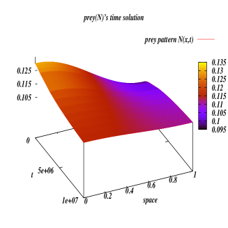
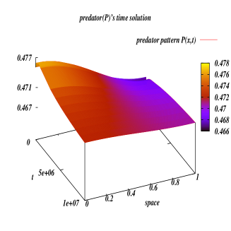
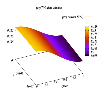
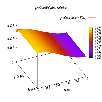
Figure 3: ($d_{1}$:0.005,$d_{2}$:0.2,$d_{c}$:0.271) Upperleft: The prey solution $N(x,t)$ with respect to time and space when $d_{2}<d_{c}$. Prey pattern shows the convergence to the equilibrium solution $N$ as time increases. Upperright: The predator solution $P(x,t)$ with respect to space when $d_{2}<d_{c}$. Predator pattern shows the convergence to the equilibrium solution $P$ as time increases.($d_{1}$:0.005,$d_{2}$:0.32,$d_{c}$:0.271) LowerLeft: The prey solution $N(x,t)$ with respect to time and space when $d_{2}>d_{c}$. Prey pattern shows the deviation from the equilibrium solution $N$ as time increases. LowerRight: The predator solution $P(x,t)$ with respect to space when $d_{2}>d_{c}$. Predator pattern shows the deviation from the equilibrium solution $P$ as time increases.

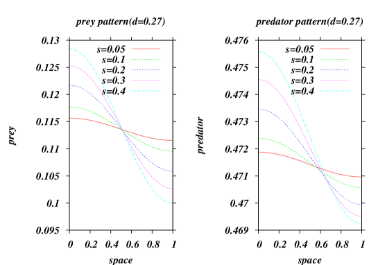
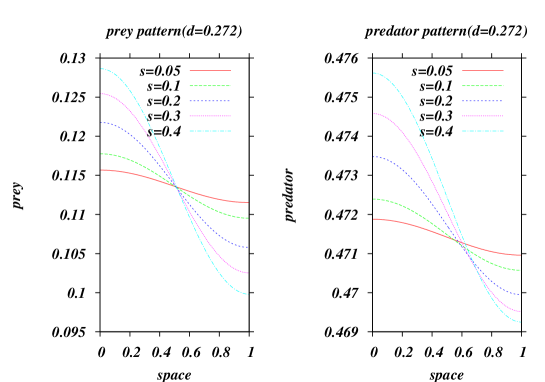
Figure 4: Upper: The prey/predator solution pattern $N(x,t),P(x,t)$ when $d_{2}<d_{c}$ with varing $s$. ($d_{1}$:0.005,$d_{2}$:0.27,$d_{c}$:0.271) Lower: The prey/predator solution pattern $N(x,t),P(x,t)$ when $d_{2}>d_{c}$. ($d_{1}$:0.005,$d_{2}$:0.272,$d_{c}$:0.271)

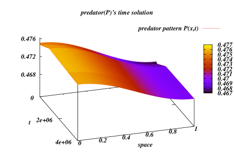
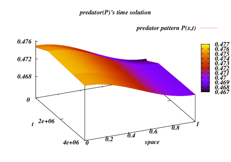
Figure 5: Upper Left: The predator solution pattern $P(x,t)$ when $s=0.1,d_{2}<d_{c}$. Upper Right: The predator solution pattern $P(x,t)$ when $s=0.4,d_{2}<d_{c}$. ($d_{1}$:0.005,$d_{2}$:0.27,$d_{c}$:0.271) Lower Left: The predator solution pattern $P(x,t)$ when $s=0.1,d_{2}>d_{c}$. Upper Right: The predator solution pattern $P(x,t)$ when $s=0.4,d_{2}>d_{c}$. ($d_{1}$:0.005,$d_{2}$:0.272,$d_{c}$:0.271)

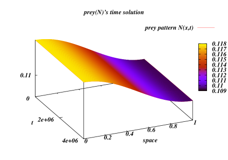
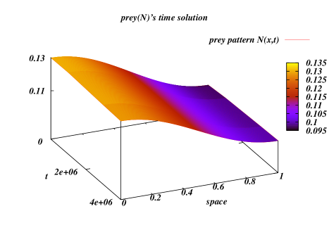
Figure 6: Upper Left: The prey solution pattern $N(x,t)$ when $s=0.1,d_{2}<d_{c}$. Upper Right: The prey solution pattern $N(x,t)$ when $s=0.4,d_{2}<d_{c}$. ($d_{1}$:0.005,$d_{2}$:0.27,$d_{c}$:0.271) Lower Left: The prey solution pattern $N(x,t)$ when $s=0.1,d_{2}>d_{c}$. Upper Right: The prey solution pattern $N(x,t)$ when $s=0.4,d_{2}>d_{c}$. ($d_{1}$:0.005,$d_{2}$:0.272,$d_{c}$:0.271)

• Figure 1 $d_{1}$ and $d_{2}$ plot, from equation (3.18)

• Figure 2 Left: The prey solution at $x$=0.25 with respect to time, the constant line represents $N_{e}=\overline{N}$ and the two solid lines represent two different $d_{2}$ values. Right: The predator solution at $x$=0.25 with respect to time, the constant line represents $P_{e}=\overline{P}$ and the two solid lines represent two different $d_{2}$ values.

• Figure 3($d_{1}$:0.005,$d_{2}$:0.2,$d_{c}$:0.271) Upperleft: The prey solution $N(x,t)$ with respect to time and space when $d_{2}<d_{c}$. Prey pattern shows the convergence to the equilibrium solution $N$ as time increases. Upperright: The predator solution $P(x,t)$ with respect to space when $d_{2}<d_{c}$. Predator pattern shows the convergence to the equilibrium solution $P$ as time increases.($d_{1}$:0.005,$d_{2}$:0.32,$d_{c}$:0.271) LowerLeft: The prey solution $N(x,t)$ with respect to time and space when $d_{2}>d_{c}$. Prey pattern shows the deviation from the equilibrium solution $N$ as time increases. LowerRight: The predator solution $P(x,t)$ with respect to space when $d_{2}>d_{c}$. Predator pattern shows the deviation from the equilibrium solution $P$ as time increases.

• Figure 4 Left: The prey/predator solution pattern $N(x,t),P(x,t)$ when $d_{2}<d_{c}$ with varing $s$. ($d_{1}$:0.005,$d_{2}$:0.27,$d_{c}$:0.271) Right: The prey/predator solution pattern $N(x,t),P(x,t)$ when $d_{2}>d_{c}$. ($d_{1}$:0.005,$d_{2}$:0.272,$d_{c}$:0.271)

• Figure 5 Upper Left: The predator solution pattern $P(x,t)$ when $s=0.1,d_{2}<d_{c}$. Upper Right: The predator solution pattern $P(x,t)$ when $s=0.4,d_{2}<d_{c}$. ($d_{1}$:0.005,$d_{2}$:0.27,$d_{c}$:0.271) Lower Left: The predator solution pattern $P(x,t)$ when $s=0.1,d_{2}>d_{c}$. Upper Right: The predator solution pattern $P(x,t)$ when $s=0.4,d_{2}>d_{c}$. ($d_{1}$:0.005,$d_{2}$:0.272,$d_{c}$:0.271)

• Figure 6 Upper Left: The prey solution pattern $N(x,t)$ when $s=0.1,d_{2}<d_{c}$. Upper Right: The prey solution pattern $N(x,t)$ when $s=0.4,d_{2}<d_{c}$. ($d_{1}$:0.005,$d_{2}$:0.27,$d_{c}$:0.271) Lower Left: The prey solution pattern $N(x,t)$ when $s=0.1,d_{2}>d_{c}$. Upper Right: The prey solution pattern $N(x,t)$ when $s=0.4,d_{2}>d_{c}$. ($d_{1}$:0.005,$d_{2}$:0.272,$d_{c}$:0.271)

References

- [1] F. Berezovskaya, G. Karev, and R. Arditi. Parametric analysis of the ratio-dependent predator-prey model. J. Math. Biol.,, 43:221–246, 2001.
- [2] S. B. Hsu, T. W. Hwang, and Y. Kuang. Global analysis of the Michaelis-Menten-type ratio-dependent predator-prey system. J. Math. Biol., 42:489–506, 2001.
- [3] C. Jost, O. Arino, and R. Arditi. About deterministic extinction in ratio-dependent predator-prey models. Bull. Math. Biol., 61:19–32, 1999.
- [4] Y. Kuang and E. Beretta. Global qualitative analysis of a ratio-dependent predator-prey system. J. Math. Biol., 36:389–406, 1998.
- [5] R. Arditi, H. R. Akcakaya, and L.R. Ginzburg. Ratio-dependent prediction: an abstraction that works. Ecology, 76:995–1004, 1995.
- [6] R. Arditi and L. R. Ginzburg. Coupling in predator-prey dynamics: ratio-dependence. J. Theor. Biol., 139:311–326, 1989.
- [7] R. Arditi, L. R. Ginzburg, and H. R. Akcakaya. Variation in plankton densities among lakes: a case for ratio-dependent models. American Naturalist, 138:1287–1296, 1991.
- [8] R. Arditi, N. Perrin, and H. Saiah. Functional response and heterogeneities: An experiment test with cladocerans. OIKOS, 60:69–75, 1991.
- [9] M. Baurmann, T. Gross, and U. Feudel. Instabilities in spatially extended predator-prey systems: spatio-temporal patterns in the neighborhood of Turing-Hopf bifurcations. J. Theoret. Biol., 245(2):220–229., 2007.
- [10] R. G. Casten and C. F. Holland. Stability properties of solutions to systems of reaction-diffusion equations. SIAM J. Appl. Math., 1977.
- [11] C. Duque and M. Lizana. Global asymptotic stability of a ratio dependent predator prey system with diffusion and delay. Period. Math. Hungar, 56(1):11–23, 2008.
- [12] P. Grindrod. Patterns and Waves The Theory and Applications of Reaction-Diffusion Equations. Clarendon Press., Oxford, 1991.
- [13] B. Mukhopadhyay and R. Bhattacharyya. Modeling the role of diffusion coefficients on turing instability in a reaction-diffusion prey-predator system. Bull. Math. Biol., 68(2):293–313, 2006.
- [14] A. Okubo and S. A. Levin. Diffusion and Ecological Problems:Modern Perspectives. Springer, Berlin, 2nd edition, 2000.
- [15] P. Y. H. Pang and M. X. Wang. Qualitative analysis of a ratio-dependent predator prey system with diffusion. Proc. R. Soc. Edinburgh A, 133(4):919–942, 2003.
- [16] M. Cavani and M. Farkas. Bifurcation in a predator-prey model with memory and diffusion II: Turing bifurcation. Acta Math. Hungar., 63:375–393, 1994.
- [17] F. Bartumeus, D. Alonso, and J. Catalan. Self organized spatial structures in a ratio dependent predator-prey model. Physica A, 295:53–57, 2001.
- [18] M. Wanga. Stationary patterns for a prey predator model with prey-dependent and ratio-dependent functional responses and diffusion. Physica D, 196:172–192, 2004.
- [19] J. Morgan. Global existence for semilinear parabolic systems via Lyapunov methods, volume 1394 of Lecture Notes in Mathematics, pages 117–121. Springer, 1989.
- [20] J. Morgan. Global existence for semilinear parabolic systems. SIAM J. Math. Anal., 1999.
- [21] J. Smoller. Shock Waves and Reaction-Diffusion Equations. Springer-Verlag, New York, Heidelberg, Berlin, 1983.
-
1.