Dynamics of the $p$-adic Shift and Applications

1. Introduction

In recent years, several authors have started studying the dynamics that result from various maps on the $p$-adics. In many cases they have shown that relatively simple and natural transformations satisfy important dynamical properties, such as ergodicity.

In this paper, we continue this line of research by studying Bernoulli transformations on the $p$-adic integers. Bernoulli transformations are those that can be identified with the “left shift” of infinite (to the right) sequences on some alphabet. They are ubiquitous throughout the field of dynamics, and come up in numerous guises in several branches of mathematics. In the realm of measurable dynamics, where we are free to disregard sets of measure zero, the map $T_{n}:[0,1]\to[0,1]$ for $n$ a positive integer, taking $x$ to $nx\bmod 1$ (i.e., the fractional part of $nx$), provides a simple example of a Bernoulli (noninvertible) transformation. Taking base-$n$ expansions of $x$, and ignoring the (measure zero) set of redundant expansions $.\overline{n-1}$, one sees that indeed this map is just a left shift.

Moving to the $p$-adic context, the aim of this paper is to present a novel way of realizing the Bernoulli shift on $p$ symbols, where $p$ is some prime. We do this by starting with the most natural realization: Any $x\in\mathbb{Z}_{p}$ has a unique (possibly infinite) expansion of the form $x=\sum_{i=0}^{\infty}b_{i}p^{i}$ ($b_{i}\in\{0,1,\ldots,p-1\}$); one can define the “$p$-adic shift” $\mathcal{S}:\mathbb{Z}_{p}\to\mathbb{Z}_{p}$ to be a left shift on this expansion, that is $\mathcal{S}(x)=\sum_{i=0}^{\infty}b_{i+1}p^{i}$. By showing that suitably small perturbations of $\mathcal{S}$ are still Bernoulli, we can find many “nice” maps, such as polynomials, that behave like the shift map $\mathcal{S}$ in this way. (We originally discussed these maps in [5]; this paper presents a novel and more direct way of obtaining them, as we will remark below.) Because we are working on the $p$-adics, our proofs use divisibility properties of certain polynomials, and thus, we obtain a connection between dynamics and number theory.

In addition to allowing us to obtain aesthetically pleasing and natural representations of Bernoulli shifts and connecting the study to number-theoretic properties like divisibility, working in the $p$-adic setting is appealing; dynamics over the $p$-adics has recently become an active area of research. Our work was motivated by the article [1], which studied the measurable dynamics of polynomial maps on $\mathbb{Z}_{p}.$ The authors in [1] asked when polynomial maps can satisfy the measurable dynamical property of being mixing. (It turns out that this was known to Woodcock and Smart, who showed in [9] that the polynomial map $x\mapsto\tfrac{x^{p}-x}{p}$ defines a Bernoulli, hence mixing, transformation on $\mathbb{Z}_{p}$.) In [5], the authors gave a detailed account of the dynamics that can result from a certain well-behaved class of maps on the $p$-adics. In particular, we introduced a set of conditions on the Mahler expansion of a transformation on the $p$-adics which are sufficient for it to be Bernoulli (see Definition 4.12).

The sufficiency of these conditions was proved in [5] via a structure theorem for so-called “locally scaling” transformations (see Definition 4.1). The Mahler-Bernoulli class conditions mentioned above were (roughly) that the transformation be a small enough perturbation of $x\mapsto\binom{x}{p}$ (which are part of the Mahler basis), and so applying the structure theorem required a careful study of the dynamics of the map $x\mapsto\binom{x}{p}$. The approach of the present paper turns out to be more direct than that of [5], to which it is in a sense dual: we begin with the easily understood dynamics of $\mathcal{S}$ and work to better understand its Mahler expansion, proving that it is “a small enough perturbation” of $x\mapsto\binom{x}{p}$. Since we are working in an ultrametric setting, this means that the Mahler-Bernoulli class condition may be reformulated as exactly those things that are small enough perturbations of $\mathcal{S}$, giving a more conceptual reason why they should be Bernoulli!

This paper is organized as follows. After a brief review of the $p$-adics, we begin by studying the $p$-adic shift and its properties. Section 4 is devoted to developing our machinery and proving the main result. We introduce locally scaling transformations (similarly to our discussion in [5]) and then show that what we mean when we say that certain maps are small perturbations of the shift map. At the end of the section, we prove that certain locally scaling transformations are indeed small perturbations of the shift map, and hence Bernoulli. In particular, we define the Mahler-Bernoulli class and show that all members thereof satisfy these properties. Finally, in Section 5 we briefly talk about maps related to the $p$-adic shift.

We have discussed locally scaling transformations and their dynamical properties in [5]. However, the interpretation that certain locally scaling transformations are in some sense small perturbation on the shift map, and therefore remain Bernoulli, is original to this paper (and is its main contribution).

Some basic familiarity with the $p$-adics, as provided, for example, in [3] or [6], will be helpful. The monograph [4] may be consulted for an introduction to $p$-adic dynamics. For measurable dynamics properties such as mixing the reader may consult [7]. Finally, [8] introduces more extensive connections between dynamics and arithmetic.

Acknowledgments

This paper is based on research by the Ergodic Theory group of the 2005 SMALL summer research project at Williams College. Support for the project was provided by National Science Foundation REU Grant DMS – 0353634 and the Bronfman Science Center of Williams College.

2. The $p$-adics

Throughout the paper, we fix a prime $p$.

2.1. The $p$-adic integers $\mathbb{Z}_{p}$

The $p$-adic integers generalize the notion of base-$p$ expansion of nonnegative integers. For any nonnegative integer $n,$ we can write down a base-$p$ expansion of $n,$ i.e., an expression $n=b_{0}+b_{1}p+b_{2}p^{2}+\cdots+b_{N}p^{N}$ where the $b_{i}$ are in $\{0,1,\ldots,p-1\}.$ Thus, the nonnegative integers are precisely the finite power series in $p$ with coefficients in $\{0,1,\ldots,p-1\}.$

The $p$-adic integers $\mathbb{Z}_{p}$ can be thought of as infinite series in a formal variable $\text{``}p\text{''},$ with the same coefficients as above: i.e., as a set we can define

$$\mathbb{Z}_{p}\stackrel{{\scriptstyle\text{def}}}{{=}}\left\{a_{0}+a_{1}\text{``}p\text{''}+\cdots+a_{i}{\text{``}p\text{''}}^{i}+\cdots=\sum_{i}a_{i}{\text{``}p\text{''}}^{i}:a_{i}\in\{0,1,\ldots,p-1\}\text{ for all $i\geq 0$}\right\}.$$

We can turn $\mathbb{Z}_{p}$ into a metric space by introducing a distance function $d:\mathbb{Z}_{p}\times\mathbb{Z}_{p}\to\mathbb{R},$ where

$$d\left(\sum_{i}a_{i}{\text{``}p\text{''}}^{i},\sum_{i}b_{i}{\text{``}p\text{''}}^{i}\right)=\begin{cases}0&\text{if $a_{i}=b_{i}$ for all $i\geq 0$}\\ p^{-k}&\text{ where $k=\min\{i\geq 0:a_{i}\neq b_{i}\}$, otherwise}\end{cases}$$

In other words, the distance between two points is small if their their expansions agree to many terms. One checks that $d(\cdot,\cdot)$ is indeed a metric on $\mathbb{Z}_{p}$, making it a complete metric space. We may also define a function $\left|\cdot\right|:\mathbb{Z}_{p}\to\mathbb{R}$ by

$$\left|\sum_{i}a_{i}{\text{``}p\text{''}}^{i}\right|=d\left(\sum_{i}a_{i}{\text{``}p\text{''}}^{i},\sum_{i}0{\text{``}p\text{''}}^{i}\right)=\begin{cases}0&\text{if $a_{i}=0$ for all $i\geq 0$}\\ p^{-k}&\text{where $k=\min\{i\geq 0:a_{i}\neq 0\}$, otherwise}\end{cases}$$

This will be our discrete valuation, though we can’t make sense of this notion without defining the ring structure. We will alternately refer to $\left|\cdot\right|$ as the $p$-adic absolute value. It is not hard to see that for any $u,v\in\mathbb{Z}_{p},$ we have $d(u,v)=|u-v|.$

Remark 2.1.

We note that $\mathbb{Z}_{p}$ is also often constructed as the metric space completion of $\mathbb{Z}$ with respect to the $p$-adic valuation $\left|\cdot\right|$. However, we would still need the “base $p$ expansions,” so might as well start from this viewpoint.

We now define the ring structure on $\mathbb{Z}_{p}.$ To do this, we consider the functions $\pi_{k}:\mathbb{Z}_{p}\to\mathbb{Z}/p^{k}\mathbb{Z}$ given by

$$\pi_{k}\left(\sum_{i}a_{i}{\text{``}p\text{''}}^{i}\right)=\left(\sum_{i=0}^{k-1}a_{i}p^{i}\right)+p^{k}\mathbb{Z}.$$

Observe that they are compatible with the natural projections $\mathbb{Z}/p^{k}\mathbb{Z}\to\mathbb{Z}/p^{\ell}\mathbb{Z}$ for $\ell<k$, and that

$$\bigcap_{k\geq 0}\pi_{k}^{-1}\left(\pi_{k}\left(\sum_{i}a_{i}{\text{``}p\text{''}}^{i}\right)\right)=\left\{\sum_{i}a_{i}{\text{``}p\text{''}}^{i}\right\}.$$

This allows us to conclude that there is a unique ring structure on $\mathbb{Z}_{p}$ for which each $\pi_{k}$ is a ring homomorphism. (In fact, readers familiar with inverse limits can see that the $\pi_{k}$ realize $\mathbb{Z}_{p}$ as the inverse limit $\mathop{\varprojlim}_{k}\mathbb{Z}/p^{k}\mathbb{Z}$ where $\mathbb{Z}/p^{k}\to\mathbb{Z}/p^{\ell}$ is the natural projection for $\ell<k$.)

The verification of this fact is not hard from the above two observations, so we will simply describe the ring operations rather than give a formal proof: To compute the first $k$ coefficients of

$$\left(\sum_{i}a_{i}{\text{``}p\text{''}}^{i}\right)+\left(\sum_{i}b_{i}{\text{``}p\text{''}}^{i}\right)\qquad\left(\text{resp., }\left(\sum_{i}a_{i}{\text{``}p\text{''}}^{i}\right)\cdot\left(\sum_{i}b_{i}{\text{``}p\text{''}}^{i}\right)\right)$$

one applies $\pi_{k}$ to each term, adds (resp., multiplies) the resulting elements of $\mathbb{Z}/p^{k}\mathbb{Z}$, and takes the first $k$ digits of the base $p$-expansion of any representative class of the result (noting that the first $k$ digits are independent of choice of representative).

With this description, we see that the function $\iota:\mathbb{Z}\to\mathbb{Z}_{p}$ given by taking an integer to its formal base $p$ expansion is precisely the unit ring homomorphism $n\mapsto n\cdot 1$. So, suppose $\sum_{i}a_{i}{\text{``}p\text{''}}^{i}$ is such that $a_{i}=0$ for $i\gg 0$. Then, the sum $\sum_{i}a_{i}p^{i}$ makes sense as an integer and

$$\sum_{i}a_{i}{\text{``}p\text{''}}^{i}=\iota\left(\sum_{i}a_{i}p^{i}\right)=\sum_{i}\iota(a_{i})\iota(p)^{i}.$$

Suppose now that $\sum_{i}a_{i}{\text{``}p\text{''}}^{i}\in\mathbb{Z}_{p}$ is arbitrary. It is the limit, in the metric space topology, of its truncated expansions (formal partial sums). Thus we can, and will, forever remove the quotes around ${\text{``}p\text{''}}$ and regard the infinite sum as a convergent sum rather than a formal expression, all with no ambiguity. Thus, we have defined $\mathbb{Z}_{p}$ as a complete discrete valuation ring; it is not hard to see that $\mathbb{Z}_{p}$ has $\mathbb{Z}$ as a dense subset.

We may also wish to ask what the units in $\mathbb{Z}_{p}$ are (i.e., for what $u\in\mathbb{Z}_{p}$ does there exist a $v$ in $\mathbb{Z}_{p}$ such that $uv=1$). It is not too difficult to show that $\mathbb{Z}_{p}^{\times}=\{u\in\mathbb{Z}_{p}:|u|=1\},$ i.e., all $p$ adic integers with nonzero $p^{0}$ coefficient.

2.2. Some $p$-adic properties

As a metric space, $\mathbb{Z}_{p}$ satisfies some unusual properties. First of all, we have the strong triangle inequality: if $u,v,w\in\mathbb{Z}_{p},$ then it is the case that $|u-v|\leq\max(|u|,|v|).$ From this, it is not hard to see that if $|u|>|v|,$ then $|u+v|=|u|.$ Furthermore, this implies that a series $\sum a_{m}$ converges if and only if $|a_{n}|\to 0.$

In our work, balls in the $p$-adic integers play a fundamental role. We define the (closed) ball of radius $r$ about $u\in\mathbb{Z}_{p}$ as $B_{r}\left(u\right)=\{v\in\mathbb{Z}_{p}:|u-v|\leq r\}.$ Because $p$-adic distances are all powers of $p,$ we may take $r=p^{i}$ for some $i$ without loss of generality. Notice that if $u=a_{0}+a_{1}p+a_{2}p^{2}+\cdots\in\mathbb{Z}_{p},$ then $B_{p^{-i}}\left(u\right)=a_{0}+a_{1}p+a_{2}p^{2}+\cdots+a_{i-1}p^{i-1}+p^{i}\mathbb{Z}_{p},$ i.e., $B_{p^{-i}}\left(u\right)$ consists of all elements of $\mathbb{Z}_{p}$ agreeing with the $p$-adic expansion of $u$ to the $p^{i-1}$ term. Using the strong triangle inequality, it is easy to see that if $u^{\prime}\in B_{p^{i}}\left(u\right),$ then $B_{p^{-i}}\left(u\right)=B_{p^{i}}\left(u^{\prime}\right)$ (thus “every point in a ball is its center”), and further, that if two balls intersect, then one is contained in the other. The $p$-adic integers form the unit ball around any element of $\mathbb{Z}_{p}.$

Additionally, it is not difficult to see that for $j\geq i,$ each ball of radius $p^{-j}$ contains $p^{j-i}$ disjoint balls of radius $i.$ In particular, each ball is totally bounded, and being closed, is compact.

2.3. Brief introduction to $\mathbb{Q}_{p}$

The set $\mathbb{Q}_{p}$ is the field of fractions of $\mathbb{Z}_{p},$ i.e.,

$$\mathbb{Q}_{p}\stackrel{{\scriptstyle\text{def}}}{{=}}\mathbb{Z}_{p}[1/p]=\bigcup_{i\geq 0}p^{-i}\mathbb{Z}_{p}.$$

Any element of $\mathbb{Q}_{p}$ can be written as a Laurent series in $p,$ with finitely many negative powers but possibly infinitely many positive ones. Alternately, just like $\mathbb{Z}_{p}$ is the completion of $\mathbb{Z}$ under the $p$-adic metric, $\mathbb{Q}_{p}$ is the completion of $\mathbb{Q}$ under this same metric. (To define $|\cdot|$ on $\mathbb{Q},$ note that any element of $\mathbb{Q}$ can be written uniquely as $s=p^{\ell}a/b,$ where $p$ divides neither $a$ nor $b$; in this case, $|s|=p^{-\ell}$.)

The set $\mathbb{Q}_{p}$ possesses many of the same properties as $\mathbb{Z}_{p}$ (for example, the strong triangle inequality).

2.4. Examples

Example 2.2.

In the $2$-adics, $1+2+4+8+\cdots=1/(1-2)=-1.$ Indeed, we can see that the difference between each successive partial sum and $-1$ becomes divisible by increasing powers of $2,$ and consequently, becomes “smaller.”

What if we had wanted to derive the $2$-adic representation of $-1$? Notice that for each $m,$ we have $-1=1+2+2^{2}+\cdots+2^{m-1}\bmod 2^{m}.$ The complete $2$-adic expansion follows.

Example 2.3.

Let us try to find a zero of the polynomial $q(x)=x^{2}+1$ in $\mathbb{Z}_{5}.$ Notice that $q(2)=5\in B_{1/5}\left(0\right).$ So, $x=2$ is an approximation to a zero of $q.$

How do we get a better approximation? More precisely, we would like to find a “small” $t$ such that $q(2+t)\in B_{1/25}\left(0\right).$ By “small,” we mean small in the $5$-adic sense; in this case, we will require $t\equiv 0\bmod 5.$

Let us write down the formal Taylor series $q(2+t)=q(2)+tq^{\prime}(2)+\cdots,$ where the dots represent terms of order at least $2$ in $t$ (hence, a contribution that is equal to $0$ mod $25$). We notice that $q^{\prime}(2)\neq 0\bmod 5,$ and so, we see that

$$t=\frac{q(2+t)-q(t)}{q^{\prime}(2)}+\cdots.$$

We require $q(2+t)\equiv 0\bmod 25,$ and know that $q(2)\equiv 5\bmod 25.$ Because $q^{\prime}(2)=4\not\equiv 0\bmod 5,$ this determines $t$ modulo $25$; the concealed terms are all $0$ modulo $25,$ and thus do not affect the result at this stage. In particular, $t\equiv 20/4\bmod 25,$ so $t\equiv 5\bmod 25.$ And indeed, $q(2+1\cdot 5)\equiv 0\bmod 25.$

Proceeding in this way, we can find $a_{0},a_{1},a_{2},\ldots\in\{0,1,2,3,4\}$ such that $q(a_{0}+a_{1}5+a_{2}5^{2}+\cdots+a_{k}5^{k})\equiv 0\bmod 5^{k+1}.$ It follows that for $\alpha=a_{0}+a_{1}5+a_{2}5^{2}+\cdots\in\mathbb{Z}_{5},$ we have $q(\alpha)=0,$ since the partial sums provide successively better approximations for the zero of $q.$

This example demonstrated a specific instance of Hensel’s Lemma, a general result about finding zeros of polynomials in $\mathbb{Z}_{p}$ [3].

3. The $p$-adic Shift

The $p$-adic shift $f:\mathbb{Z}_{p}\longrightarrow\mathbb{Z}_{p}$ is defined as follows. If $x=b_{0}+b_{1}p+b_{2}p^{2}+\cdots,$ where the $b_{i}\in\{0,1,\ldots,p-1\},$ we let $\mathcal{S}(x)=b_{1}+b_{2}p+b_{3}p^{2}+\cdots.$ We immediately see that if $\mathcal{S}^{k}$ denotes the $k$-fold iterate of $\mathcal{S},$ then we have that $\mathcal{S}^{k}(x)=b_{k}+b_{k+1}p+\cdots.$ Moreover, for $x\in\mathbb{Z},$ it is the case that $\mathcal{S}^{k}(x)=\left\lfloor x/p^{k}\right\rfloor$ where $\left\lfloor\cdot\right\rfloor$ is the greatest integer function.

One of the most basic properties of the shift is that it is continuous as a function of $\mathbb{Z}_{p}.$ Indeed, if $|x-y|<1/p^{k+1},$ it is not hard to see that $|\mathcal{S}(x)-\mathcal{S}(y)|<1/p^{k}.$ (Recall that $\left|\cdot\right|$ is the $p$-adic absolute value.)

Continuity is important because by Mahler’s Theorem, any continuous $T:\mathbb{Z}_{p}\longrightarrow\mathbb{Z}_{p}$ can be expressed in the form of a uniformly convergent series, called its Mahler Expansion:

(1) $$T(x)=\sum_{n=0}^{\infty}a_{n}\binom{x}{n}$$

where

(2) $$a_{n}=\sum_{i=0}^{n}(-1)^{n+i}T(i){n\choose i}\in\mathbb{Z}_{p}$$

Remark 3.1.

For an arbitrary function $T:\mathbb{Z}_{p}\to\mathbb{Z}_{p},$ we can write down the formal identity $T(x)=\sum_{n=0}^{\infty}a_{n}{x\choose n}$ for coefficients $a_{n}\in\mathbb{Z}_{p}$ to be determined. Then, substituting in $x=0,1,2,\ldots$ in turn, we can inductively determine that the $a_{n}$ would have to be as in (2), noting that only finitely many summands will be non-zero at each stage. The true content of Mahler’s Theorem is that for $T$ continuous on $\mathbb{Z}_{p},$ this series converges, which happens if and only if $|a_{n}|\to 0$ as $n\to\infty$ by convergence properties on the $p$-adics.

Our first goal is to study the Mahler expansion of $\mathcal{S}^{k}.$ Throughout this paper, we let $a_{n}^{(k)}$ be the $n^{\text{th}}$ Mahler coefficient of $\mathcal{S}^{k}.$ In other words, the $a_{n}^{(k)}$ are defined such that

(3) $$\mathcal{S}^{k}(x)=\sum_{n=0}^{\infty}a_{n}^{(k)}\binom{x}{n}.$$

Theorem 3.2.

The coefficients $a_{n}^{(k)}$ satisfy the following properties:

1. $a_{n}^{(k)}=0$ for $0\leq n<p^{k}$;

2. $a_{n}^{(k)}=1$ for $n=p^{k}$;

3. Suppose $j\geq 0$. Then, $p^{j}$ divides $a_{n}^{(k)}$ for $n>jp^{k}-j+1$ (and so, $|a_{n}^{(k)}|\leq 1/p^{j}$).

Proof.

Our proof is closely based on Elkies’s short derivation of Mahler’s Theorem [2]. Let

$$F(t)=\sum_{n\geq 0}\mathcal{S}^{k}(n)t^{n}\in\mathbb{Z}_{p}[[t]]\qquad\text{and}\qquad A(u)=\sum_{n\geq 0}a_{n}^{(k)}u^{n}\in\mathbb{Z}_{p}[[u]].$$

Recall the standard power series identities

$$\frac{1}{1-t}=\sum_{i\geq 0}t^{i}\qquad\text{and}\qquad\frac{t}{(1-t)^{2}}=\sum_{i\geq 1}it^{i}.$$

Using them and the definition of $\mathcal{S}^{k},$ we may compute that

$$F(t) =\sum_{n\geq 0}\mathcal{S}^{k}(n)t^{n}=\sum_{a=0}^{p^{k}-1}\sum_{b\geq 0}bt^{a+bp^{k}}$$

$$=\left(\sum_{a=0}^{p^{k}-1}t^{a}\right)\left(\sum_{b\geq 0}b(t^{p^{k}})^{b}\right)=\left(\frac{1-t^{p^{k}}}{1-t}\right)\left(\frac{t^{p^{k}}}{(1-t^{p^{k}})^{2}}\right)$$

$$=\frac{t^{p^{k}}}{(1-t)(1-t^{p^{k}})}$$

Before proceeding, we remark that

(4) $$A(u)=\frac{1}{1+u}F\left(\frac{u}{1+u}\right).$$

Indeed, suppose $T:\mathbb{Z}_{p}\to\mathbb{Q}_{p}$ is any map. Set $\tilde{F}(t)=\sum_{n\geq 0}T(n)t^{n}$ and $\tilde{A}(u)=\sum_{n\geq 0}a_{n}u^{n}$ where $a_{n}$ is such that $\sum_{i}a_{i}\binom{n}{i}=T(n)$ for all $k\geq 0$. Then,

$$\tilde{F}(t) =\sum_{n\geq 0}\sum_{i=0}^{n}a_{i}\binom{n}{i}t^{n}=\sum_{i\geq 0}a_{i}\sum_{n\geq i}\binom{n}{i}t^{n}=\sum_{i\geq 0}a_{i}\frac{t^{i}}{(1-t)^{i+1}}$$

$$=\left(\frac{1}{1-t}\right)\sum_{i\geq 0}a_{i}\left(\frac{t}{1-t}\right)^{i}=\frac{1}{1-t}\tilde{A}\left(\frac{t}{1-t}\right)$$

From this, (4) follows by taking $\tilde{F}=F,$ $\tilde{A}=A,$ and $t=u/(1+u).$

Now, note that because $p|\binom{p^{k}}{i}$ for all $0<i<p^{k},$ we have $(1+u)^{p^{k}}-u^{p^{k}}=1+pR(u)$ where $R(u)$ is a polynomial of degree $p^{k}-1$ in $u$ without leading term, so that

$$A(u)=\frac{1}{1+u}F\left(\frac{u}{1+u}\right)=\frac{u^{p^{k}}}{(1+u)^{p^{k}}-u^{p^{k}}}=u^{p^{k}}\left(1+pR(u)+p^{2}R(u)^{2}+p^{3}R(u)^{3}+\cdots\right)$$

Since $R(u)$ has no leading term, we can now conclude (i) and (ii). The case $j=0$ of (iii) is trivial, so we may assume $j\geq 1$. Working modulo $p^{j}$ we obtain the equality (in $\mathbb{Z}_{p}/p^{j}\mathbb{Z}_{p}[[u]]$)

$$A(u)\equiv u^{p^{k}}\left(1+pR(u)+\cdots+p^{j-1}R(u)^{j-1}\right)\pmod{p^{j}}$$

Note that the right hand side is a polynomial of degree $p^{k}+(j-1)(p^{k}-1)=jp^{k}-j+1$. This allows us to conclude (iii). ∎

As we will see, the next corollary will be of fundamental importance in the following section, where we try to bound coefficients in the Mahler expansions of maps related to the shift.

Corollary 3.3.

The maximum possible value for $p^{\left\lfloor\log_{p}n\right\rfloor}|a_{n}^{(k)}|$ is $p^{k}$ and it is attained only when $n=p^{k}.$

Proof.

We may assume $a_{n}^{(k)}\neq 0$. Let $v_{p}(a_{n}^{(k)})$ denote the integer $\ell$ so that $p^{\ell}$ precisely divides $a_{n}^{(k)}$. We are asked to prove that $\left\lfloor\log_{p}n\right\rfloor-v_{p}(a_{n}^{(k)})\leq k$ with equality if and only if $n=p^{k}$. Setting $\ell=\left\lfloor\log_{p}n\right\rfloor-k$, we are thus to show that $p^{\ell}$ divides $a_{n}^{(k)}$ and $p^{\ell+1}$ divides it unless $n=p^{k}$.

Note that $p^{\ell}\geq\ell$ so that

$$n\geq p^{\left\lfloor\log_{p}n\right\rfloor}=p^{\ell}p^{k}\geq\ell p^{k}\geq\ell p^{k}-\ell+1$$

and applying Theorem 3.2 yields that $p^{\ell}$ does in fact divide $a_{n}^{(k)}$.

If $\ell>0$, then $p^{\ell}\geq\ell+1$ so that we in fact have $n\geq(\ell+1)p^{k}\geq(\ell+1)p^{k}-(\ell+1)+1$ and so Theorem 3.2 yields that $p^{\ell+1}$ does in fact divide $a_{n}^{(k)}$. Since $a_{n}^{(k)}=0$ for $n<p^{k}$, by Theorem 3.2, it suffices to prove that $p$ divides $a_{n}^{(k)}$ for $n>p^{k}$; but this is immediate from Theorem 3.2. ∎

4. Perturbing the Shift

4.1. Local Scaling

The shift $\mathcal{S}$ cuts off the first digit term in the $p$-adic expansion of $x\in\mathbb{Z}_{p}.$ Notice that if the expansions of $x$ and $y$ agree past the the first digit (i.e., $|x-y|\leq 1/p$), $\mathcal{S}$ multiplies the distance between them by $p.$ Thus, $\mathcal{S}$ scales distances between points that are close enough.

This observation motivates the following definition from [5].

Definition 4.1.

We say that $T:\mathbb{Z}_{p}\longrightarrow\mathbb{Z}_{p}$ is locally scaling with scaling radius $r$ and scaling constant $C\geq 1,$ and write that $T$ is $(r,C)$ locally scaling if for all $x,$ $y$ with $|x-y|\leq r,$ $|T(x)-T(y)|=C|x-y|.$ We will always assume, without loss of generality, that $r=p^{\ell}$ and $C=p^{m},$ where $\ell\leq 0$ and $m\geq 0.$

Proposition 4.2.

The map $\mathcal{S}^{k}$ is $(p^{-k},p^{k})$ locally scaling.

Proof.

Immediate. ∎

Notice that if $T$ is a locally scaling map, it is continuous, and for $r^{\prime}\leq r,$ the restriction $T\left.\right|_{B_{r^{\prime}}\left(x\right)}$ is injective into $B_{Cr^{\prime}}\left(T(x)\right).$ It is surjective as well.

Proposition 4.3.

For $T$ an $(r,C)$ locally scaling map and $r^{\prime}\leq r,$ the restricted map $T\left.\right|_{B_{r^{\prime}}\left(x\right)}:B_{r^{\prime}}\left(x\right)\longrightarrow B_{Cr^{\prime}}\left(T(x)\right)$ is a bijection.

Proof.

Let $S=T\left.\right|_{B_{r^{\prime}}\left(x\right)}.$ Because injectivity of $S$ is clear, we just prove surjectivity. We first demonstrate that the image of $S$ is dense in $B_{Cr^{\prime}}\left(T(x)\right)$ by showing that for every ball $B\subset B_{Cr^{\prime}}\left(T(x)\right)$ there exists $w\in B_{r^{\prime}}\left(x\right)$ such that $T(w)\in B.$ Say the radius of $B$ is $p^{-j}\leq Cr^{\prime}$ for $j\in\mathbb{Z}_{\geq 0}.$

Assume furthermore that there are $\eta$ balls of radius $(1/C)\,p^{-j}$ contained in $B_{r^{\prime}}\left(x\right).$ Pick one point in each of these balls of radius $(1/C)\,p^{-j}$ (the representative of that ball). Because these $\eta$ representatives are all at least $(1/C)\,p^{-j}$ apart from one another and $(1/C)\,p^{-j}\leq r^{\prime},$ their images have to be at least $p^{-j}$ apart from one another by local scaling. Thus, they have to occupy $\eta$ distinct balls of radius $p^{-j}$ in the range. Finally, because the number of balls of radius $p^{-j}$ contained in $B_{Cr^{\prime}}\left(T(x)\right)$ is also $\eta,$ one of the representatives in $B_{r^{\prime}}\left(x\right)$ must map into $B$ by the pigeonhole principle.

Now that we have the image of $S$ being dense in $B_{Cr^{\prime}}\left(T(x)\right),$ we note that $S$ is continuous and $B_{r^{\prime}}\left(x\right)$ is compact, so $S(B_{r^{\prime}}\left(x\right))$ must be compact hence closed. Thus it is all of $B_{Cr^{\prime}}\left(T(x)\right).$ Hence, our map is surjective and therefore bijective. ∎

4.2. $(p^{-k},p^{k})$ locally scaling maps

We now turn our attention to a special case of local scaling, the $(p^{-k},p^{k})$ locally scaling maps. We will see that they behave “nicely” under preimages. More precisely, when one takes successive preimages of a given ball, we get a union of smaller balls that are very evenly distributed throughout $\mathbb{Z}_{p}.$

Let $T$ be such a map. In this case, each of the $p^{k}$ balls of radius $p^{-k}$ is mapped bijectively onto $\mathbb{Z}_{p}.$ It follows that given a ball $B\subset\mathbb{Z}_{p},$ of radius $p^{-j}$ its preimage is

$$T^{-1}(B)=\bigsqcup_{i=1}^{p^{k}}B_{i}$$

where each $B_{i}$ is a ball of radius $p^{-(j+k)},$ and the $B_{i}$ are contained in distinct balls of radius $p^{-k}.$ Furthermore, if $B^{\prime}\subset B$ is a ball of radius $p^{-j^{\prime}}\leq p^{-j},$ then

$$T^{-1}(B^{\prime})=\bigsqcup_{i=1}^{p^{k}}B_{i}^{\prime}$$

where each $B_{i}^{\prime}$ is a ball of radius $p^{-(j^{\prime}+k)},$ and each $B_{i}^{\prime}$ is contained in $B_{i}.$ We call this very nice property of preimages the nesting property (see Figure 1 for an illustration).

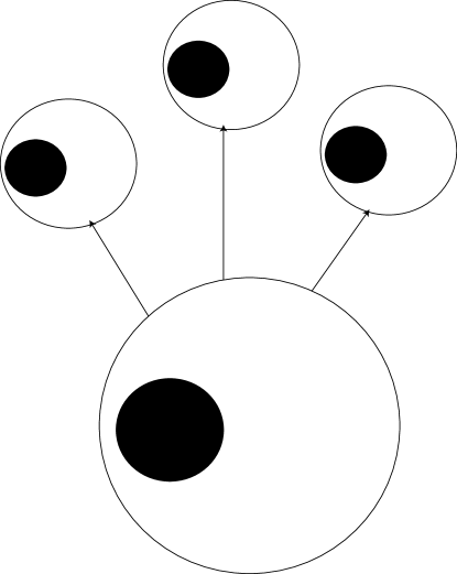
Figure 1. An illustration of the local nesting property. Let $B$ be the big ball at the bottom of the figures; the arrows lead to its preimages $B_{1},$ $B_{2},$ and $B_{3}.$ The shaded ball inside $B$ is some ball $B^{\prime}.$ Its preimages $B_{1}^{\prime},B_{2}^{\prime}$ and $B_{3}^{\prime}$ each fall within one of the $B_{i}.$

Finally, the next two lemma will play a role in our main result.

Lemma 4.4.

Suppose that $B$ is a ball of radius $p^{-kj}.$ Then, $T^{-1}(B)$ consists of a union of $p^{k}$ balls of radius $p^{-k(j+1)},$ each of them in a distinct ball of radius $p^{-kj}.$

Proof.

The preceding discussion proves everything except the last statement. So, say we have $x$ and $y$ in $T^{-1}(B),$ so that both are in the same ball of radius $p^{-kj}.$ Thus, $|x-y|\leq p^{-kj},$ so $|T(x)-T(y)|=p^{k}|x-y|.$ But, it must be the case that $|T(x)-T(y)|\leq p^{-kj},$ and this only happens when $|x-y|\leq p^{-k(j+1)}.$ It follows that $x$ and $y$ are both in the same ball of $T^{-1}(B).$ ∎

Lemma 4.5.

Let $T:\mathbb{Z}_{p}\to\mathbb{Z}_{p}$ be $(p^{-k},p^{k})$-locally scaling. Then, for any $j,n\geq 1,$ we have that

$$T^{-n}(B_{p^{-jk}}\left(y\right))=\bigcup_{\nu=1}^{p^{kn}}B_{\nu},$$

where the $B_{\nu}$ are balls of radius $p^{-k(n+j)},$ one inside each ball of radius $p^{-kn}$ in $\mathbb{Z}_{p}.$

Proof.

We proceed by induction. The base case ($n=1$) is covered by Lemma 4.4.

For the inductive step, assume that our lemma holds for $n=i.$ In other words, suppose that

$$T^{-i}\left(B_{p^{-jk}}\left(y\right)\right)=\bigcup_{\nu=1}^{p^{ki}}B_{\nu}$$

where the $B_{\nu}$ are balls of radius $p^{-k(i+j)}$ one each in every ball of radius $p^{-ki}$ of $\mathbb{Z}_{p}.$ Then, $T^{-(i+1)}\left(B_{p^{-jk}}\left(y\right)\right)=\bigcup T^{-1}(B_{\nu}).$ But, by Lemma 4.4, for each $\nu,$ we have that $T^{-1}(B_{\nu})=\bigcup_{\mu=1}^{p^{k}}C_{\mu}^{\nu},$ where each $C_{\mu}^{\nu}$ is a ball of radius $p^{-k(i+j+1)},$ one in each ball of radius $p^{k}$ of $\mathbb{Z}_{p}.$ In particular, for a given $\nu,$ the $C_{\mu}^{\nu}$ are in distinct balls of radius $p^{-k(i+1)}.$

Finally, we argue that if $C_{\mu}^{\nu}$ and $C_{\mu^{\prime}}^{\nu^{\prime}}$ are contained in the same ball of radius $p^{-k(i+1)}$, then it follows that $\nu=\nu^{\prime}$ (and so $\mu=\mu^{\prime}$ by the above argument). Indeed, say $x\in C_{\mu}^{\nu}$ and $x^{\prime}\in C_{\mu^{\prime}}^{\nu^{\prime}}$ with $|x-x^{\prime}|\leq p^{-k(i+1)}.$ Then $|T(x)-T(x^{\prime})|\leq p^{-ki}.$ But, $T(x)\in B_{\nu}$ and $T(x^{\prime})\in B_{\nu^{\prime}},$ so, since $B_{\nu}$ and $B_{\nu^{\prime}}$ are in distinct balls of radius $p^{-ki}$ unless $\nu=\nu^{\prime},$ we find that indeed $\nu=\nu^{\prime}.$

We thus see that

$$T^{-(i+1)}\left(B_{p^{-jk}}\left(y\right)\right)=\bigcup_{\nu=1}^{p^{kn}}\bigcup_{\mu=1}^{p^{k}}C_{\mu}^{\nu},$$

where the $C_{\mu}^{\nu}$ are balls of radius $p^{-k(i+j+1)},$ one each in every ball of radius $p^{-k(i+1)}$ of $\mathbb{Z}_{p}.$ The lemma thus holds for $n=i+1,$ completing the inductive step and therefore the proof. ∎

The preceding results suggest that if $T$ is $(p^{-k},p^{k})$ locally scaling and $B$ is a ball, taking $T^{-n}(B)$ for larger and larger $n$ will produce sets that are very well mixed among $\mathbb{Z}_{p}.$ In fact, we have already established enough machinery to show that $T$ is mixing with respect to the standard Haar measure $\mu$ on $\mathbb{Z}_{p}.$ The measure $\mu$ is completely specified by defining its values on balls: the $\mu$ measure of each ball is defined to be its radius. A transformation $T$ is said to be mixing if for any $\mu$-measurable sets $U$ and $V$ we have that $\lim_{n\to\infty}\mu(T^{-n}(U)\cap V)=\mu(U)\mu(V).$ It turns out, however, that it is enough to establish this in the case that $U$ is a ball of radius $p^{-kj}$ and $V$ is a ball of radius $p^{-k\ell}$ for any positive integers $j$ and $\ell$ (see e.g. [7, Theorem 6.3.4]). Taking $n\geq\ell,$ we find that $T^{-n}(U)=\bigcup B_{\nu}$ where each $B_{\nu}$ is a ball of radius $p^{-k(n+j)}$ one each in every ball of radius $p^{-kn}$ in $\mathbb{Z}_{p}.$ But there are $p^{k(n-\ell)}$ balls of radius $p^{-kn}$ in $B,$ each of them containing one $B_{\nu}.$ Therefore,

$$\mu(T^{-n}(U)\cap V) =\mu\left(\bigcup_{\nu=1}^{p^{k(n-\ell)}}B_{\nu}\right)=\sum_{\nu=1}^{p^{k(n-\ell)}}\mu(B_{\nu})$$

$$=p^{k(n-\ell)}p^{-k(n+j)}=p^{-k(\ell+j),}$$

which is equal to $\mu(U)\mu(V).$ It follows that $T$ is mixing.

We conclude this discussion with an example.

Example 4.6.

Consider the maps $S,T:\mathbb{Z}_{2}\to\mathbb{Z}_{2}$ $S(x)=\binom{x}{2}$ and $T(x)=\binom{x}{3}.$ Let us consider the preimages of $2\mathbb{Z}_{2}$ and $1+2\mathbb{Z}_{2}$ (the two balls of radius $1/2$ in $\mathbb{Z}_{2}$) under $S$ and $T.$

Now, $S(x)=x(x-1)/2.$ One of $x$ and $x-1$ will cancel out the factor of $2$ in the denominator. For $S(x)$ to be in $2\mathbb{Z}_{2},$ we need another factor of $2$ in the numerator, meaning that either $x$ or $x-1$ must be equal to $0$ modulo $4.$ In other words, $S^{-1}(2\mathbb{Z}_{2})=4\mathbb{Z}_{2}\cup(1+4\mathbb{Z}_{2}).$ On the other hand, if we want to have $S(x)\in 1+2\mathbb{Z}_{2},$ neither $x$ nor $x-1$ can be congruent to $0$ modulo $4.$ In other words, $x\equiv 2\text{ or }3\bmod 4.$ Thus, $S^{-1}(1+2\mathbb{Z}_{2})=(2+4\mathbb{Z}_{2})\cup(3+4\mathbb{Z}_{2}).$ We can thus see how taking the preimage mixes up among the two balls of radius $1/2.$

Let us now consider $T(x)=x(x-1)(x-2)/6.$ Notice that $T(x)\in 2\mathbb{Z}_{2}$ precisely if $x\equiv 0\bmod 2.$ Indeed, we then get two powers of $2$ from $x$ and $x-2,$ one of which cancels a power of $2$ from the denominator. Therefore, $T^{-1}(2\mathbb{Z}_{2})=2\mathbb{Z}_{2}.$ Likewise, $T^{-1}(1+2\mathbb{Z}_{2})=1+2\mathbb{Z}_{2}.$ So, in general, if $B$ is a ball of radius $1/2$ in $\mathbb{Z}_{2},$ then for all $n>0,$ it is the case that $T^{-n}(B)=B.$

This discussion of preimages suggests that $S$ is mixing while $T$ is not, and, as we shall see, this is indeed the case.

4.3. Connections with Bernoulli Maps

With our setup, we will be able to say that certain maps (namely the $(p^{-k},p^{k})$ locally scaling ones) in many senses behave “the same” as the $p$-adic Bernoulli shift (or one of its iterates). To make these notions more precise, we introduce some concepts in topological dynamics.

Definition 4.7.

Two maps $T:\mathbb{Z}_{p}\longrightarrow\mathbb{Z}_{p}$ and $S:\mathbb{Z}_{p}\longrightarrow\mathbb{Z}_{p}$ are said to be (topologically) isomorphic if there exists a homeomorphism $\Phi:\mathbb{Z}_{p}\longrightarrow\mathbb{Z}_{p}$ such that $\Phi\circ T(x)=S\circ\Phi(x)$ for all $x.$ In other words, $\Phi$ conjugates the action of $T$ to the action of $S.$

Close variants of the following theorem and proof are in [5].

Theorem 4.8.

Let $T:\mathbb{Z}_{p}\longrightarrow\mathbb{Z}_{p}$ be a $(p^{-k},p^{k})$ locally scaling map. Then, $T$ is topologically isomorphic to $\mathcal{S}^{k}.$

Proof.

We must find a homeomorphism $\Phi:\mathbb{Z}_{p}\longrightarrow\mathbb{Z}_{p}$ such that $\Phi\circ T=\mathcal{S}^{k}\circ\Phi.$ Consider

$$\Phi(x)=\sum_{i=0}^{\infty}d_{i}(x)p^{i},$$

where, if $i=qk+r$ for $0\leq r<k,$ we have that $d_{i}(x)=(T^{q}(x))_{r}$ (the $r$th digit in the $p$-adic expansion of $T^{q}(x)$). From this definition, it is easy to see that $\Phi\circ T(x)=\mathcal{S}^{k}\circ\Phi(x)$ for all $x\in\mathbb{Z}_{p}.$

We now proceed to show that $\Phi,$ as defined, is continuous and bijective. Because $\mathbb{Z}_{p}$ is compact, continuity of the inverse follows by general facts in topology. Therefore, we will have proved that $\Phi$ is a homeomorphism.

To show that $\Phi$ is continuous, suppose that $|x-y|\leq p^{-k\eta}$ for $\eta\geq 1.$ It follows by local scaling that $|T(x)-T(y)|\leq p^{-k(\eta-1)},$ and in general, we can see that for $q\leq\eta-1,$ we have that $|T^{q}(x)-T^{q}(y)|\leq p^{-k}.$ Therefore, the $p$-adic expansions of $\Phi(x)$ and $\Phi(y)$ agree at least up to the $p^{-(k\eta-1)}$ term, and we see that $|\Phi(x)-\Phi(y)|\leq p^{-k\eta}.$ Continuity follows.

To show injectivity, suppose that $\Phi(x)=\Phi(y).$ Then, $|T^{i}(x)-T^{i}(y)|\leq p^{-k}$ for all $i\geq 0.$ But if $|T^{i}(x)-T^{i}(y)|\neq 0$ for some $i,$ it follows by local scaling that there is a $j\geq 0$ such that $|T^{i+j}(x)-T^{i+j}(y)|>p^{-k},$ a contradiction.

Finally, we prove surjectivity. Suppose that $y\in\mathbb{Z}_{p},$ and we want to find an $x\in\mathbb{Z}_{p}$ such that $\Phi(x)=y.$ From the definition of $\Phi,$ we see that we are looking for an $x$ such that

$$x \in B_{p^{-k}}\left(y\right)$$

$$T(x) \in B_{p^{-k}}\left(\mathcal{S}^{k}(y)\right)$$

$$T^{2}(x) \in B_{p^{-k}}\left(\mathcal{S}^{2k}(y)\right)$$

$$\vdots$$

$$T^{i}(x) \in B_{p^{-k}}\left(\mathcal{S}^{ik}(y)\right)$$

$$\vdots$$

Therefore, to prove that $\Phi$ is surjective, we have to show that for all $y\in\mathbb{Z}_{p},$ the intersection

$$\bigcap_{i\geq 0}T^{-i}\left(B_{p^{-k}}\left(\mathcal{S}^{ik}(y)\right)\right)$$

is nonempty.

And indeed, by Lemma 4.5, for $i\geq 1,$ each ball of $T^{-i}\left(B_{p^{-k}}\left(\mathcal{S}^{ik}(y)\right)\right)$ contains exactly one ball of $T^{-(i+1)}\left(B_{p^{-k}}\left(\mathcal{S}^{(i+1)k}(y)\right)\right).$ Furthermore, one ball of $T^{-1}\left(B_{p^{-k}}\left(y\right)\right)$ is contained in $B_{p^{-k}}\left(y\right).$ These considerations show that an intersection of any finite subcollection of the $T^{-i}\left(B_{p^{-k}}\left(\mathcal{S}^{ik}(y)\right)\right)$ is nonempty, and therefore, by compactness of $\mathbb{Z}_{p},$ we have that

$$\bigcap_{i\geq 0}T^{-i}\left(B_{p^{-k}}\left(\mathcal{S}^{ik}(y)\right)\right)\neq\emptyset,$$

as required. ∎

4.4. “Small” Perturbations on $\mathcal{S}^{k}$

At this point in the presentation, we have determined that $(p^{-k},p^{k})$ maps are Bernoulli. Furthermore, by understanding the Mahler expansion of the shift map $\mathcal{S}^{k},$ as we did earlier, we hope to understand the scaling properties of polynomial maps (namely, finite $\mathbb{Z}_{p}$-linear combinations of the $\binom{x}{n}$), and thus, to find Bernoulli polynomials. As we will see, we have an infinite class of polynomial maps such that any $g$ in this class can be written as a sum of $\mathcal{S}^{k}$ and a perturbing factor satisfying the Lipschitz property (see below). In turn, this perturbing factor has small enough Lipschitz constant so that $g$ is $(p^{-k},p^{k})$ locally scaling, like $\mathcal{S}^{k}.$ We proceed to lay the groundwork for this argument.

Definition 4.9.

We say that a function $T:\mathbb{Z}_{p}\longrightarrow\mathbb{Z}_{p}$ is $C$-Lipschitz if $|T(x)-T(y)|\leq C|x-y|$ for all $x,y\in\mathbb{Z}_{p}.$

If $T$ is $C$-Lipschitz and $a\in\mathbb{Q}_{p},$ it is clear that $aT$ is $|a|C$-Lipschitz. Also, because of the strong triangle inequality, if $T_{i}$ is $C_{i}$-Lipshitz, $\sum T_{i}$ is $(\sup_{i}\{C_{i}\})$-Lipshitz, provided this supremum exists (i.e., the $C_{i}$ are bounded).

Lipshitz maps are important in our discussion because they provide us with a way of slightly modifying a locally scaling function such that the resulting map is still locally scaling. The following proposition demonstrates one such method.

Proposition 4.10.

Let $T:\mathbb{Z}_{p}\longrightarrow\mathbb{Z}_{p}$ be $(r,C)$ locally scaling, $S:\mathbb{Z}_{p}\longrightarrow\mathbb{Z}_{p}$ be $D$-Lipshitz with $D<C,$ and suppose that $u\in\mathbb{Z}_{p}^{\times}.$ Then $\tilde{T}=uT+S$ is $(r,C)$-locally scaling.

Proof.

Take $x$ and $y$ with $|x-y|\leq r.$ Then

(5) $$|\tilde{T}(x)-\tilde{T}(y)| = |(uT(x)+S(x))-(uT(y)+S(y))|$$

(6) $$= |u(T(x)-T(y))+(S(x)-S(y))|.$$

But, $|u(T(x)-T(y))|=C|x-y|>D|x-y|\geq|S(x)-S(y)|.$ Therefore, $|\tilde{T}(x)-\tilde{T}(y)|=C|x-y|,$ as desired. ∎

In particular, if $\tilde{f}(x)=\mathcal{S}^{k}(x)+b(x)$ where $b$ is $p^{k-1}$-Lipshitz, then $\tilde{f}$ is $(p^{-k},p^{k})$ locally scaling, and hence Bernoulli. This seemingly uninspiring condition is actually extremely powerful because it gives us sufficient conditions on the Mahler expansion of a continuous map $T:\mathbb{Z}_{p}\longrightarrow\mathbb{Z}_{p}$ for the map to be isomorphic to $\mathcal{S}^{k}$ for some $k.$

Before stating the result, however, we need the following lemma, which we do not prove here:

Lemma 4.11.

The $\mathbb{Z}_{p}$ map $x\mapsto{x\choose n}$ is $p^{\left\lfloor\log_{p}n\right\rfloor}$-Lipshitz for all $n.$

Proof.

See [6, pg. 227]. ∎

Definition 4.12.

Let $T(x)$ be given by the uniformly converging Mahler series

$$T(x)=\sum_{n=0}^{\infty}A_{n}{x\choose n}$$

and set $C=\max_{n}p^{\left\lfloor\log_{p}n\right\rfloor}|A_{n}|.$ Suppose that the following conditions hold:

• There exists a unique $n_{0}$ which attains this maximum;

• $n_{0}=p^{k}$ for some $k>0$;

• $|A_{n_{0}}|=1$ (thus, $C=n_{0}=p^{k}$).

Then, we say that $T$ is in the Mahler-Bernoulli class.

Theorem 4.13.

Let $T$ be in the Mahler-Bernoulli class, with $C=p^{k}$ as in the definition. Then $T$ is $(p^{-k},p^{k})$ locally scaling and hence isomorphic to $\mathcal{S}^{k}.$

Proof.

A variant of this theorem is in [5]. The proof that follows uses the Mahler expansion of $\mathcal{S}^{k},$ and is original to this paper.

The idea of the proof is that by the Mahler-Bernoulli class conditions, the $A_{p_{k}}\binom{x}{p^{k}}$ term will be the dominant one in determining the scaling behavior of $T.$ Indeed, as we will see below, after multiplying by a unit as appropriate, $T$ and $\mathcal{S}^{k}$ differ by a $p^{k-1}$-Lipshitz component; this follows by the Mahler-Bernoulli class conditions, as well as the tight control guaranteed by Lemma 4.11. The details of this argument follow.

Recall that for the map $\mathcal{S}^{k},$ we have that $a^{(k)}_{p^{k}}=1.$ Therefore, the fact that $|A_{p_{k}}|=1$ in the Mahler expansion of $T$ implies that there exists $u\in\mathbb{Z}_{p}^{\times}$ such that $ua_{p^{k}}^{(k)}=A_{p_{k}}.$ Consider the general term $b_{n}=ua_{n}^{(k)}-A_{n}.$ By choice of $u,$ we have $b_{p^{k}}=0.$ Furthermore, the strong triangle inequality tells us that $|b_{n}|\leq\max\{|a_{n}^{(k)}|,A_{n}\}.$ Regardless of what the maximum is for a particular $n\neq p^{k},$ it is the case that $|b_{n}|p^{\left\lfloor\log_{p}n\right\rfloor}<p^{k}$ by definition and Corollary 3.3. Therefore, using Lemma 4.11, we see that $b_{n}{x\choose n}$ is $p^{k-1}$-Lipshitz for all $n$ (since $b_{p^{k}}=0,$ the claim is trivial for $b=p^{k}$).

Hence, $u\mathcal{S}^{k}(x)-T(x)=\sum_{n=0}^{\infty}b_{n}{x\choose n}$ is $p^{k-1}$-Lipshitz. This implies, by Proposition 4.10, that $T$ is $(p^{-k},p^{k})$ locally scaling and the theorem follows. ∎

Remark 4.14.

The reader may (rightly) point out that proving the local scaling properties of maps like $\binom{x}{p^{k}}$ should not be much harder than proving Lipschitz properties of the $\binom{x}{n}.$ Indeed, this was done directly in [5]. Going through the Mahler expansion of the shift map provides us with not as much a new proof of the local scaling properties, but an interpretation of the maps in the Mahler-Bernoulli class, which satisfy them.

5. Other Related Maps

The $p$-adic shift is actually a special case of another natural class of maps. First off, define $g:\mathbb{Q}_{p}\longrightarrow\mathbb{Z}_{p}$ as follows. Given $x\in\mathbb{Q}_{p},$ we can express it uniquely as $x=\sum_{i=\ell}^{\infty}b_{i}p^{i}$ where $\ell\leq 0$ and $b_{i}\in\{0,1,\ldots,p-1\}$ for all $i.$

With our setup notation, we let $g(x)=\sum_{i=0}^{\infty}b_{i}p^{i}.$ In other words, $g$ chops off the negative powers of $p$ in the $p$-adic expansion of $x.$

Take $a\in\mathbb{Q}_{p}.$ Define $f_{a}:\mathbb{Z}_{p}\longrightarrow\mathbb{Z}_{p}$ by $f_{a}(x)=g(ax)$ where $g$ is as above. Notice that the $p$-adic shift is $f_{a}$ where $a=1/p.$

We will mostly be interested in $f_{a}$ with $|a|>1.$ Now, $|a|>1$ implies that $a=a^{\prime}/p^{k}$ for $a^{\prime}\in\mathbb{Z}_{p}^{\times}$ and $k>0.$ Therefore, for $x\in\mathbb{Z}_{p},$ $f_{a}(x)=g(a^{\prime}x/p^{k})$ where $a^{\prime}x\in\mathbb{Z}_{p}$ and so, $f_{a}(x)=\mathcal{S}^{k}(a^{\prime}x).$

We now make a few remarks about the topological dynamics of the maps $f_{a}.$

For $a$ with $|a|<1,$ we have that $f_{a}(\mathbb{Z}_{p})\subsetneq\mathbb{Z}_{p},$ so $f_{a}$ is not surjective, and cannot be isomorphic to the shift.

The situation when $|a|>1$ is quite different.

Theorem 5.1.

For $|a|=p^{k},$ with $k>0,$ $f_{a}$ is $(p^{-k},p^{k})$ locally scaling, and hence isomorphic to $\mathcal{S}^{k}.$

Proof.

We know that $f_{a}(x)=\mathcal{S}^{k}(a^{\prime}x)$ where $a^{\prime}\in\mathbb{Z}_{p}^{\times}.$ Take $x$ and $y$ with $|x-y|\leq p^{-k}.$ Then, $|a^{\prime}x-a^{\prime}y|=|x-y|\leq p^{-k}.$ Therefore, $|\mathcal{S}^{k}(a^{\prime}x)-\mathcal{S}^{k}(a^{\prime}y)|=p^{k}|a^{\prime}x-a^{\prime}y|=p^{k}|x-y|$ and so $f_{a}$ is $(p^{-k},p^{k})$ locally scaling. ∎

References

- [1] John Bryk and Cesar E. Silva, Measurable dynamics of simple -adic polynomials, Amer. Math. Monthly 112 (2005), no. 3, 212–232.
- [2] Noam D. Elkies, Mahler’s theorem on continuous -adic maps via generating functions, http://www.math.harvard.edu/elkies/Misc/mahler.pdf.
- [3] Fernando Q. Gouvêa, -adic numbers, Universitext, Springer-Verlag, Berlin, 1993, An introduction. MR MR1251959 (95b:11111)
- [4] Andrei Yu. Khrennikov and Marcus Nilsson, -adic deterministic and random dynamics, Kluwer, 2004.
- [5] James Kingsbery, Alex Levin, Anatoly Preygel, and Cesar E. Silva, On measure-preserving transformations of compact-open subsets of non-Archimedean local fields, Trans. Amer. Math. Soc. 361 (2009), no. 1, 61–85. MR MR2439398
- [6] Alain M. Robert, A course in -adic analysis, Graduate Texts in Mathematics, vol. 198, Springer-Verlag, New York, 2000. MR MR1760253 (2001g:11182)
- [7] C. E. Silva, Invitation to ergodic theory, Student Mathematical Library, vol. 42, American Mathematical Society, Providence, RI, 2008.
- [8] Joseph H. Silverman, The arithmetic of dynamical systems, Graduate Texts in Mathematics, vol. 241, Springer, New York, 2007. MR MR2316407 (2008c:11002)
- [9] Christopher F. Woodcock and Nigel P. Smart, -adic chaos and random number generation, Experiment. Math. 7 (1998), no. 4, 333–342.