Abstract

We derive the non-universal gaugino mass ratios in a supergravity (SUGRA) framework where the Higgs superfields belong to the non-singlet representations 54 and 770 in an $SO(10)$ Grand Unified Theory (GUT). We evaluate the ratios for the phenomenologically viable intermediate breaking chain $SU(4)_{C}\times SU(2)_{L}\times SU(2)_{R}~{}(G_{422})$. After a full calculation of the gaugino mass ratios, noting some errors in the earlier calculation for 54, we obtain, using the renormalisation group equations (RGE), interesting low scale phenomenology of such breaking patterns. Here, we assume the breaking of the $SO(10)$ GUT group to the intermediate gauge group and that to the Standard Model (SM) take place at the GUT scale itself. We also study the collider signatures in multilepton channels at the Large Hadron Collider (LHC) for some selected benchmark points allowed by the cold dark matter relic density constraint provided by the WMAP data and compare these results with the minimal supergravity (mSUGRA) framework with similar gluino masses indicating their distinguishability in this regard.

1 Introduction

With the Large Hadron Collider (LHC) about to be operative shortly, the search for physics beyond the standard model (SM) has reached a new height of excitement. Low energy (TeV scale) supersymmetry (SUSY) has persistently remained one of the leading candidates among scenarios beyond the Standard Model (SM), not only because of its attractive theoretical framework, but also for the variety of phenomenological implications it offers [1, 2, 3, 4]. The stabilization of the electroweak symmetry breaking (EWSB) scale and the possibility of having a cold dark-matter (CDM) candidate with conserved $R$-parity ($R=(-1)^{(3B+L+2S)}$) [5] are a few elegant phenomenological features of SUSY. Side by side, the possibility of paving the path towards a Grand Unified Theory (GUT) is one of its most exciting theoretical prospects, where one can relate the $SU(3)$, $SU(2)$ and $U(1)$ gauge couplings and the corresponding gaugino masses at a high scale [4, 6, 7].

The most popular framework of SUSY-breaking is the minimal supergravity (mSUGRA) scheme, where SUSY is broken in the ’hidden sector’ via gravity mediation and as a result, one can parametrise all the SUSY breaking terms by a universal gaugino mass ($M_{1/2}$), a universal scalar mass ($m_{0}$), a universal trilinear coupling parameter $A_{0}$, the ratio of the vacuum expectation values ($vev$) of the two Higgses ($\tan\beta$) and the sign of the SUSY-conserving Higgs mass parameter, ($sgn(\mu)$) [4, 8].

However, within the ambit of a SUGRA-inspired GUT scenario itself, one might find some deviations from the above-mentioned simplified and idealized situations mentioned above. For instance, the gaugino mass parameter ($M_{1/2}$) or the common scalar mass parameter ($m_{0}$) can become non-universal at the GUT scale. In this particular work, we adhere to a situation with non-universal gaugino masses in a supersymmetric scenario embedded in $SO(10)$ GUT group.

Gaugino masses, arising after GUT-breaking and SUSY-breaking at a high scale, crucially depend on the gauge kinetic function, as discussed in the next section. One achieves universal gaugino masses if the hidden sector fields (Higgses, in particular), involved in GUT-breaking, are singlets under the underlying GUT group. However if we include the higher dimensional terms (dimension five, in particular) in the non-trivial expansion of the gauge-kinetic function, the Higgses belonging to the symmetric products of the adjoint representation of the underlying GUT group can be non-singlets. If these non-singlet Higgses are responsible for GUT breaking, the gaugino masses $M_{1}$, $M_{2}$ and $M_{3}$ become non-universal at the high scale itself. It is also possible to have more than one non-singlet representations involved in GUT breaking, in which case the non-universality arises from a linear combination of the effects mentioned above.

Although this issue has been explored in earlier works, particularly in context of the $SU(5)$ [9, 10, 11], there had been one known effort [12] to study the same in context of the $SO(10)$. In this paper, we calculate the non-universal gaugino mass ratios for the non-singlet representations 54 and 770, based on the results obtained in [13], for the intermediate gauge group, namely, Pati-Salam gauge group ${SU(4)}_{c}\times{SU(2)}_{L}\times{SU(2)}_{R}~{}~{}(G_{422})$ with conserved $D$-parity [14]. In order to understand the low-energy phenomenology of such high scale breaking patterns, which is indeed essential in context of the LHC and dark matter searches, we scan a wide region of parameter space using the renormalisation group equations (RGE) and discuss the consequences in terms of various low-energy constraints. For example, we discuss the consistency of such low-energy spectra with the radiative electroweak symmetry breaking (REWSB), Landau pole, tachyonic masses etc. We also point out the constraints from stau-LSP (adhering to a situation with conserved $R$-parity and hence lightest neutralino- LSP), and flavour constraints like $b\rightarrow s\gamma$ for all possible combination of the parameter space points. Here, we assume the breaking of the $SO(10)$ to the intermediate gauge group and that to SM takes place at the GUT scale. To study the collider signatures in context of the LHC, we choose some benchmark points (BP) consistent with the cold dark matter [5] relic density constraint obtained from the WMAP data [15]. We perform the so-called ’multilepton channel analysis’ [16, 17] in $same-sign~{}dilepton$, $opposite-sign~{}dilepton$, $trilepton$, $inclusive~{}four-lepton$ channels associated with $jets$, as well as in $hadronically~{}quiet~{}trilepton$ channel at these benchmark points. We compare our results with WMAP allowed points in mSUGRA, tuned at the same gluino masses .

There has been a lot of effort in discussing various phenomenological aspects [18, 19, 20, 21, 22] of such high scale non-universality and its effect in terms of collider signatures [23, 24, 25], our analysis is remarkable in the following aspects:

• Apart from noting some errors in the earlier available calculations of non-universal gaugino mass ratio for the representation 54, we present the hitherto unknown ratio for the representation 770 for the intermediate breaking chain $G_{422}$.

• While we discuss the consistency of the low-energy spectra obtained from such high scale non-universality in a wide region of the parameter space, we study the collider aspects as well in some selected BPs in context of the LHC.

• In order to distinguish such non-universal schemes from the universal one, we compare our results at these chosen BPs with WMAP allowed points in mSUGRA tuned at the same gluino masses. We identify a remarkable distinction between the two, which might be important in pointing out the departure in ‘signature-space’ [26, 27, 28, 29] in context of the LHC for different input schemes at the GUT scale.

The paper is organized as follows. In the following section, we calculate the non-universal gaugino mass ratios. The low-energy spectra, their constancy with various constraints and subsequently the choices of the BPs have been discussed in section 3. Section 4 contains the strategy of the collider simulation and the numerical results obtained. We conclude in section 5.

2 Non-universal Gaugino mass ratios for $SO(10)$

Here we calculate the non-universal gaugino mass ratios for non-singlet Higgses belonging to the representations 54 and 770 under $SO(10)$ SUSY-GUT scenario.

We adhere to a situation where all soft SUSY breaking effects arise via hidden sector interactions in an underlying supergravity (SUGRA) framework, specifically, in $SO(10)$ gauge theories with an arbitrary chiral matter superfield content coupled to N=1 supergravity.

All gauge and matter terms including gaugino masses in the N=1 supergravity Lagrangian depend crucially on two fundamental functions of chiral superfields [30]: (i) gauge kinetic function $f_{\alpha\beta}(\Phi)$, which is an analytic function of the left-chiral superfields $\Phi_{i}$ and transforms as a symmetric product of the adjoint representation of the underlying gauge group ($\alpha$, $\beta$ being the gauge indices, run from 1 to 45 for $SO(10)$ gauge group); and (ii) $G(\Phi_{i},\Phi^{*}_{i})$, a real function of $\Phi_{i}$ and gauge singlet, with $G=K+ln|W|$ ($K$ is the K$\ddot{a}$hler potential and $W$ is the superpotential).

The part of the N=1 supergravity Lagrangian containing kinetic energy and mass terms for gauginos and gauge bosons (including only terms containing the real part of $f(\Phi)$) reads

$$e^{-1}{\mathcal{L}}=-\frac{1}{4}Ref_{\alpha\beta}(\phi)(-1/2\bar{\lambda}^{\alpha}D\!\!\!\!/\lambda^{\beta})-\frac{1}{4}Ref_{\alpha\beta}(\phi)F_{\mu\nu}^{\alpha}F^{\beta\mu\nu}$$

$$+\frac{1}{4}e^{-G/2}G^{i}((G^{-1})^{j}_{i})[\partial f^{*}_{\alpha\beta}(\phi^{*})/\partial{\phi^{*j}}]\lambda^{\alpha}\lambda^{\beta}+h.c$$ (1)

where $G^{i}=\partial{G}/\partial{\phi_{i}}$ and $(G^{-1})^{i}_{j}$ is the inverse matrix of ${G^{j}}_{i}\equiv\partial{G}/{\partial{\phi^{*i}}\partial{\phi_{j}}}$, $\lambda^{\alpha}$ is the gaugino field, and $\phi$ is the scalar component of the chiral superfield $\Phi$, and $F_{\mu\nu}^{\alpha}$ is defined in unbroken $SO(10)$. The $F$-component of $\Phi$ enters the last term to generate gaugino masses with a consistent SUSY breaking with non-zero $vev$ of the chosen $\tilde{F}$, where

$$\tilde{F}^{j}=\frac{1}{2}e^{-G/2}[G^{i}((G^{-1})^{j}_{i})]$$ (2)

The $\Phi^{j}$ s can be a set of GUT singlet supermultiplets $\Phi^{S}$, which are part of the hidden sector, or a set of non-singlet ones $\Phi^{N}$, fields associated with the spontaneous breakdown of the GUT group to $SU(3)\times SU(2)\times U(1)$ . The non-trivial gauge kinetic function $f_{\alpha\beta}(\Phi^{j})$ can be expanded in terms of the non-singlet components of the chiral superfields in the following way

$$f_{\alpha\beta}(\Phi^{j})=f_{0}(\Phi^{S})\delta_{\alpha\beta}+\sum_{N}\xi_{N}(\Phi^{s})\frac{{\Phi^{N}}_{\alpha\beta}}{M}+{\mathcal{O}}(\frac{\Phi^{N}}{M})^{2}$$ (3)

where $f_{0}$ and $\xi^{N}$ are functions of chiral singlet superfields, essentially determining the strength of the interaction and $M$ is the reduced Planck mass$=M_{Pl}/\sqrt{8\pi}$.

In Equation (3), the contribution to the gauge kinetic function from $\Phi^{N}$ has to come through symmetric products of the adjoint representation of the associated GUT group, since $f_{\alpha\beta}$ on the left side of Equation (3) has such transformation property for the sake of gauge invariance.

For $SO(10)$, one can have contributions to $f_{\alpha\beta}$ from all possible non-singlet irreducible representations to which $\Phi^{N}$ can belong :

$$(45\times 45)_{symm}=1+54+210+770$$ (4)

As an artifact of the expansion of the gauge kinetic function $f_{\alpha\beta}$ mentioned in Equation (3), the gauge kinetic term (2nd term) in the Lagrangian (Equation (1)) can be recast in the following form

$$Ref_{\alpha\beta}(\phi)F_{\mu\nu}^{\alpha}F^{\beta\mu\nu}=\frac{\xi_{N}(\Phi^{s})}{M}Tr(F_{\mu\nu}\Phi^{N}F^{\mu\nu})$$ (5)

where $F_{\mu\nu}$, under unbroken $SO(10)$, contains $U(1)_{Y}$, $SU(2)_{L}$ and $SU(3)_{C}$ gauge fields.

Next, the kinetic energy terms are restored to the canonical form by rescaling the gauge superfields, by defining

$${F^{\alpha}}_{\mu\nu}\rightarrow{\hat{F}^{\alpha}}_{\mu\nu}={\langle Ref_{\alpha\beta}\rangle}^{\frac{1}{2}}{F^{\beta}}_{\mu\nu}$$ (6)

and

$$\lambda^{\alpha}\rightarrow{\hat{\lambda}}^{\alpha}={\langle Ref_{\alpha\beta}\rangle}^{\frac{1}{2}}\lambda^{\beta}$$ (7)

Simultaneously, the gauge couplings are also rescaled (as a result of Equation (3)):

$$g_{\alpha}(M_{X}){\langle Ref_{\alpha\beta}\rangle}^{\frac{1}{2}}\delta_{\alpha\beta}=g_{c}(M_{X})$$ (8)

where $g_{c}$ is the universal coupling constant at the GUT scale ($M_{X}$). This shows clearly that the first consequence of a non-trivial gauge kinetic function is non-universality of the gauge couplings $g_{\alpha}$ at the GUT scale [9, 10, 31, 32].

Once SUSY is broken by non-zero $vev$’s of the $\tilde{F}$ components of hidden sector chiral superfields, the coefficient of the last term in Equation (1) is replaced by [9, 10]

$${\langle{\tilde{F}_{\alpha\beta}}^{i}\rangle}={\mathcal{O}}(m_{\frac{3}{2}}M)$$ (9)

where $m_{\frac{3}{2}}=exp(-\frac{\langle G\rangle}{2})$ is the gravitino mass. Taking into account the rescaling of the gaugino fields (as stated earlier in Equation (7)) in Equation (1), the gaugino mass matrix can be written down as [9, 11]

$$M_{\alpha}(M_{X})\delta_{\alpha\beta}=\sum_{i}\frac{{\langle F^{i}_{\acute{\alpha}\acute{\beta}}\rangle}}{2}\frac{\langle\partial{f_{\alpha\beta}(\phi^{*i})}/\partial{{\phi^{*i}}_{\acute{\alpha}\acute{\beta}}}\rangle}{\langle Ref_{\alpha\beta}\rangle}$$ (10)

which demonstrates that the gaugino masses are non-universal at the GUT scale.

The underlying reason for this is the fact that $\langle f_{\alpha\beta}\rangle$ can be shown to acquire the form $f_{\alpha}\delta_{\alpha\beta}$, where the $f_{\alpha}$ ’s are purely group theoretic factors, as we will see. On the contrary, if symmetry breaking occurs via gauge singlet fields only, one has $f_{\alpha\beta}=f_{0}\delta_{\alpha\beta}$ from Equation (3) and as a result, $\langle f_{\alpha\beta}\rangle=f_{0}$. Thus both gaugino masses and the gauge couplings are unified at the GUT scale (as can be seen from Equations (8) and (10)).

As mentioned earlier, we would like to calculate here, the $f_{\alpha}$ ’s for Higgses ($\Phi^{N}$) belonging to the representations 54 and 770 which break $SO(10)$ to the intermediate gauge group $SU(4)_{C}\times SU(2)_{L}\times SU(2)_{R}$ with unbroken $D$-parity (usually denoted as $G_{422P}$) . We associate the non-universal contributions to the gaugino mass ratios with the group theoretic coefficients $f_{\alpha}$ ’s that arise here. It in turn, indicates that we consider the non-universality in the gaugino masses of $O(1)$. This, however, is not a generic situation in such models. This can be rather achieved under some special conditions like dynamical generation of SUSY-breaking scale from the electroweak scale, no soft-breaking terms for the GUT or Planck scale particles and with the simplified assumption $M_{GUT}=M_{Pl}$ which is also reflected in the RGE specifications.

The representations of $SO(10)$ [33], decomposed into that of the Pati-Salam gauge group are

$$SO(10) \rightarrow G_{422}=SU(4)_{C}\times SU(2)_{L}\times SU(2)_{R}$$

$${\bf 45} \rightarrow ({\bf 15},{\bf 1},{\bf 1})\oplus({\bf 1},{\bf 3},{\bf 1})\oplus({\bf 1},{\bf 1},{\bf 3})\oplus({\bf 6},{\bf 2},{\bf 2})$$

$${\bf 10} \rightarrow ({\bf 6},{\bf 1},{\bf 1})\oplus({\bf 1},{\bf 2},{\bf 2})$$ (11)

$${\bf 16} \rightarrow ({\bf 4},{\bf 2},{\bf 1})\oplus({\bf\bar{4}},{\bf 1},{\bf 2})$$

Using the $SO(10)$ relation, ($10\times 10$) = $1+45+54$, one can see that $vev$ of 54-dimensional Higgs (${\langle 54\rangle}$) can be expressed as a (10 $\times$ 10) diagonal traceless matrix. Thus the non-zero $vev$ of 54-dimensional Higgs can be written as [32]

$$<54>=\frac{v_{54}}{2\sqrt{15}}~{}diag(3,3,3,3,,-2,-2,-2,-2,-2,-2).$$ (12)

Since $(45\times 45)_{sym}=1+54+210+770$, one can write the non-zero $vev$ [13] of 770-dimensional Higgs as ($45\times 45$) diagonal matrix:

$${\langle 770\rangle}=\frac{v_{770}}{\sqrt{180}}~{}diag(\underbrace{-4,......,-4}_{15},\underbrace{-10,...,-10}_{3+3},\underbrace{5,......,5}_{24})$$ (13)

In the intermediate scale ($M_{C}$), $G_{422}$ is broken to SM gauge group. Here $SU(4)_{C}$ is broken down to $SU(3)_{C}\times U(1)_{B-L}$ and at the same time, $SU(2)_{R}$ is broken to $U(1)_{T_{3}R}$. It is noted that $SU(2)_{R}\times SU(4)_{C}$ is broken to $SU(3)_{C}\times U(1)_{Y}$ and hence the hypercharge is given as $Y=T_{3R}+\frac{1}{2}(B-L)$. Below we note the branchings of $SU(4)_{C}$ representations:

$$SU(4)_{C} \rightarrow SU(3)_{C}\times U(1)_{B-L}$$

$${\bf 4} \rightarrow {\bf 3}_{1/3}\oplus{\bf 1}_{-1}$$

$${\bf 15} \rightarrow {\bf 8}_{0}\oplus{\bf 3}_{4/3}\oplus{\bf\bar{3}}_{-4/3}\oplus{\bf 1}_{0}$$ (14)

$${\bf 10} \rightarrow {\bf 6}_{2/3}\oplus{\bf 3}_{-2/3}\oplus{\bf 1}_{-2}$$

$${\bf 6} \rightarrow {\bf 3}_{-2/3}\oplus{\bf\bar{3}}_{2/3}$$

Combining these together, we achieve the branchings of $SO(10)$ representations in terms of the SM gauge group.

$$SO(10) :SU(3)_{C}\times SU(2)_{L}\times U(1)_{Y}$$

$${\bf 45} :$$

$$({\bf 15},{\bf 1},{\bf 1}) \rightarrow({\bf 8},{\bf 1})_{0}\oplus({\bf 3},{\bf 1})_{2/3}\oplus({\bf\bar{3}},{\bf 1})_{-2/3}\oplus({\bf 1},{\bf 1})_{0}$$

$$({\bf 1},{\bf 3},{\bf 1}) \rightarrow({\bf 1},{\bf 3})_{0}$$

$$({\bf 1},{\bf 1},{\bf 3}) \rightarrow({\bf 1},{\bf 1})_{1}\oplus({\bf 1},{\bf 1})_{0}\oplus({\bf 1},{\bf 1})_{-1}$$

$$({\bf 6},{\bf 2},{\bf 2}) \rightarrow({\bf 3},{\bf 2})_{1/6}\oplus({\bf 3},{\bf 2})_{-5/6}\oplus({\bf\bar{3}},{\bf 2})_{5/6}\oplus({\bf\bar{3}},{\bf 2})_{1/6}$$

$${\bf 10} :$$

$$({\bf 6},{\bf 1},{\bf 1}) \rightarrow({\bf 3},{\bf 1})_{-1/3}\oplus({\bf\bar{3}},{\bf 1})_{1/3}$$

$$({\bf 1},{\bf 2},{\bf 2}) \rightarrow({\bf 1},{\bf 2})_{1/2}\oplus({\bf 1},{\bf 2})_{-1/2}$$

$${\bf 16} :$$

$$({\bf 4},{\bf 2},{\bf 1}) \rightarrow({\bf 3},{\bf 2})_{1/6}\oplus({\bf 1},{\bf 2})_{-1/2}$$

$$({\bf\bar{4}},{\bf 1},{\bf 2}) \rightarrow({\bf\bar{3}},{\bf 1})_{1/3}\oplus({\bf\bar{3}},{\bf 1})_{-2/3}\oplus({\bf 1},{\bf 1})_{1}\oplus({\bf 1},{\bf 1})_{0}$$ (17)

We have $U(1)_{T_{3R}}$ and $U(1)_{B-L}$ from $SU(2)_{R}$ and $SU(4)_{C}$ respectively. Thus the weak hyper-charge generator ($T_{Y}$) can be expressed as a linear combination of the generators of $SU(2)_{R}$ ($T_{3R}$) and $SU(4)_{C}$ ($T_{B-L}$) sharing the same quantum numbers. In 10-dimensional representation $T_{3R}$, $T_{B-L}$ and $T_{Y}$ are written as:

$$T_{3R}=diag(0,0,0,0,0,0,\frac{1}{2},-\frac{1}{2},\frac{1}{2},-\frac{1}{2})$$ (18)

$$T_{B-L}=\sqrt{\frac{3}{2}}diag(-\frac{1}{3},-\frac{1}{3},-\frac{1}{3},\frac{1}{3},\frac{1}{3},\frac{1}{3},0,0,0,0)$$ (19)

$$T_{Y}=\sqrt{\frac{3}{5}}diag(-\frac{1}{3},-\frac{1}{3},-\frac{1}{3},\frac{1}{3},\frac{1}{3},\frac{1}{3},\frac{1}{2},-\frac{1}{2},\frac{1}{2},-\frac{1}{2})$$ (20)

Using these explicit forms of the generators we find the following relation

$$T_{Y}=\sqrt{\frac{3}{5}}T_{3R}+\sqrt{\frac{2}{5}}T_{B-L}$$ (21)

and this leads to the following mass relation,

$$M_{1}=\frac{3}{5}~{}M_{2R}+\frac{2}{5}~{}M_{4C}$$ (22)

• For 54-dimensional Higgs:

Using 54-dimensional Higgs we have [32], for $D$-parity even scenario, $M_{4C}=1$ and $M_{2R}=M_{2L}=-\frac{3}{2}$. We have identified that $M_{3}=M_{4C}$ and $M_{2}=M_{2R}$. Hence, using the above mass relation we obtain $M_{1}=-\frac{1}{2}$. Therefore the gaugino mass ratio is given as:

$$M_{1}:M_{2}:M_{3}=(-\frac{1}{2}):(-\frac{3}{2}):1$$ (23)

We have already mentioned that the $vev$ [13] of 770-dimensional Higgs can be expressed as a ($45\times 45$) diagonal matrix. So to calculate the gaugino masses, using 770-dimensional Higgs, we repeat our previous task in 45-dimensional representation. The explicit forms of $T_{Y}$, $T_{B-L}$ and $T_{3R}$ are noted in the Appendix and find the same mass relation as in Equation (22)

$$M_{1}=\frac{3}{5}~{}M_{2R}+\frac{2}{5}~{}M_{4C}$$ (24)

This mass relation among the $U(1)_{Y}$, $SU(2)_{L}$ and $SU(3)_{C}$ gauginos are independent of dimensions and representations.

• 770-dimensional Higgs:

Using 770-dimensional Higgs we find [13] for $D$-parity even case $M_{4C}=2$ and $M_{2R}=M_{2L}=5$. Hence, using the above mass relation we obtain $M_{1}=3.8$. Therefore the gaugino mass ratio is given as:

$$M_{1}:M_{2}:M_{3}=1.9:2.5:1$$ (25)

We tabulate the gaugino mass ratios, obtained above, in Table 1.

Representation	$M_{3}:M_{2}:M_{1}$ at $M_{GUT}$
1	1:1:1
54: $H\rightarrow SU(4)\times SU(2)\times SU(2)$	1:(-3/2):(-1/2)
770: $H\rightarrow SU(4)\times SU(2)\times SU(2)$	1:(2.5):(1.9)

Table 1: High scale gaugino mass ratios for the representations 54 and 770.

Now we would like to address the question whether the $D$-Parity Odd case is phenomenologically viable. We know, if we use 210-dimensional Higgs instead of 54 or 770, the $D$-parity is broken by $vev$ of 210 dimensional Higgs when $SO(10)\longrightarrow SU(4)_{C}\times SU(2)_{L}\times SU(2)_{R}$. This has a nice feature: $M_{2L}=-M_{2R}$ and $M_{4C}=0$, which implies that at high scale $M_{3}$ will be zero. We have analyzed the running of such high scale parameters numerically and found that these cases are not phenomenologically viable. With $M_{3}=0$ at high scale, we will, always, hit Landau pole i.e. we will be in non-perturbative regime after running down to the low scale. This is not only the specialty of 210-dimensional Higgs, but also true for all the $D$-parity breaking scenarios. Hence we conclude that the $D$-parity non-conserving scenario doesn’t fit into the non-universal gaugino mass framework, in particular, when we are bothered about a MSSM spectrum valid at the EWSB scale.

2.1 Implication of the Intermediate Scale

We have an underlying assumption that the breaking of $SO(10)$ GUT group to the intermediate gauge group and that to the SM takes place at the GUT scale itself, which is of course a simplification. But more interesting question to ask is how things will change if the intermediate scale is different from the GUT scale (which is usually the most realistic one)? Although we do not address this question in this analysis, we prefer to mention the crucial consequences of choosing an intermediate scale distinctly different from GUT scale:

• In this case, the choice of the non-singlet Higgses will be restricted. Now, only those Higgses will contribute which have a singlet direction under the intermediate gauge group. Hence, the Higgses that break $SO(10)$ directly to the SM at the GUT scale are disallowed. The choices of the non-singlet Higgses, in our analysis, are compatible even if the intermediate scale is different from the GUT scale.

• The mass relation in Equation (22) is indeed independent of the intermediate scale as it is an outcome of purely group theoretical analysis. But the gaugino mass ratios will change depending on the choice of the intermediate scale due to the running of the gaugino masses from the GUT scale.

3 Low energy spectra, Consistency and Benchmark Points

Before we discuss in details the low-energy spectra for the non-universal inputs, we would like to mention a few points regarding the evolution of these gaugino mass ratios with different RGE specifications. As we know, in the one-loop RGE, the gaugino mass parameters do not involve the scalar masses [34], the ratios obtained at the low scale are independent of the high scale scalar mass input $m_{0}$. In addition, if we also assume no radiative corrections (R.C) to the gaugino masses, the ratios at the EWSB scale are also independent of the choice of the gaugino mass parameters at the high scale. Instead, if one uses the two-loop RGE (scalars contributing to the gauginos), the values of the gaugino masses at the EWSB scale tend to decrease compared to the values obtained with one-loop RGE. Now, independently, the inclusion of R.C to the gaugino masses, makes the $M_{3}$ lower, but the values of $M_{1}$ and $M_{2}$ become higher compared to the case of one-loop results with no R.C. When, one uses both the two-loop RGE and R.C to the gauginos, it is a competition between these two effects. In short, the gaugino mass ratios at the EWSB scale crucially depend on the choice of the RGE specifications. However, the dependence on the high scale mass parameters $m_{0}$ and/or $M_{3}$ is very feeble.

We present in Table 2, the gaugino mass ratios at the EWSB scale for two different RGE conditions:

• One-loop RGE with no R.C to the gaugino masses

• Two-loop RGE with R.C to the gaugino masses

Representation	$M_{3}:M_{2}:M_{1}$	$M_{3}:M_{2}:M_{1}$
	one-loop with No R.C	two-loop with R.C
1 (mSUGRA)	1:0.27:0.13	1:0.35:0.19
54: $H\rightarrow SU(4)\times SU(2)\times SU(2)$	1:(-0.40):(-0.06)	1:(-0.55):(-0.10)
770: $H\rightarrow SU(4)\times SU(2)\times SU(2)$	1:0.67:0.24	1:0.91:0.37

Table 2: Low scale (EWSB) gaugino mass ratios for representations 54 and 770.

The numerical results have been obtained using the spectrum generator SuSpect v2.3 [36] with the pMSSM option. For the rest of our analysis we adhere to the second type of RGE specifications, two-loop RGE + R.C to the gauginos as mentioned earlier. The other broad specifications used for the scanning are listed below.

• Full one-loop and the dominant two-loop corrections to the Higgs masses are incorporated.

• Gauge coupling constant unification at the high scale have been ensured and the corresponding scale has been chosen as the ’high scale’ or ’GUT-scale’ to start the running by RGE. All the non-universal inputs are provided at this scale using the pMSSM option. This is an artifact of choosing the intermediate scale set at the GUT scale itself.

• Electroweak symmetry breaking at the ‘default scale’ $\sqrt{m_{\tilde{t_{L}}}m_{\tilde{t_{R}}}}$ has been set.

• We have used the strong coupling ${\alpha_{3}(M_{Z})}^{\overline{MS}}=0.1172$ for this calculation which is again the default option in SuSpect.

• Throughout the analysis we have assumed the top quark mass to be 171.4 GeV.

• All the scalar masses have been set to a universal value of $m_{0}$ and radiative electroweak symmetry breaking has been taken into account by setting high scale Higgs mass parameter ${M_{H_{u}}}^{2}={M_{H_{d}}}^{2}={m_{0}}^{2}$ and specifying $sgn(\mu)$, which has been taken to be positive throughout the analysis.

• All the trilinear couplings have been set to zero.

• Tachyonic modes for sfermions and other inconsistencies in RGE, like Landau pole have been taken into account.

• As we work in a $R$-parity conserving scenario, stau-LSP regions have been identified as disfavoured.

• Consistency with low-energy FCNC constraints such as those from $b\rightarrow s\gamma$ has been noted for each combination of the parameter space. We have used a 3$\sigma$ level constraint from $b\rightarrow s\gamma$ with the following limits [37].

  $$2.77\times 10^{-4}<Br(b\rightarrow s\gamma)<4.33\times 10^{-4}.$$ (26)

  However, we must point out that we have taken all those regions as allowed where the value of $b\rightarrow s\gamma$ is lower or within the constraint.

• Regions allowed by all these constraints have been studied for the relic density constraint of the cold dark matter (CDM) candidate (lightest neutralino in our case) and referred to the the WMAP data [15] within 3$\sigma$ limit

  $$0.091<\Omega_{CDM}h^{2}<0.128.$$ (27)

  where $\Omega_{CDM}h^{2}$ is the dark matter relic density in units of the critical density and $h=0.71\pm 0.026$ is the Hubble constant in units of $100\ \rm Km\ \rm s^{-1}\ \rm Mpc^{-1}$.

We have used the code microOMEGA v2.0.7 [38] for computing the relic density.

With these inputs, we scan the parameter space for a wide range of values of $m_{0}$ and $M_{3}$ for the non-universal gaugino mass ratios advocated above.

The ratios obtained for 54 at the high scale (see Table 1) are actually the same as the one for the representation 24 in case of $SU(5)$ (see [9, 10, 11, 24]). This observation differs from the earlier result available in [12]. The low-energy spectrum and its consistency for the case of 24 have been well-studied [21]. Without the inclusion of the intermediate breaking scale in case of $SO(10)$, the case of 54 is difficult to distinguish from the one in $SU(5)$. Anyway we do not address any such situations here and hence, refrain from illustrating the case of 54.

In Figure 1, we depict the results of the scan in the $M_{3}-m_{0}$ parameter space for the representation 770, i.e. breaking through $G_{422}$. Along the x-axis, high scale $M_{3}$ is varied from 100-2000 GeV and along the y-axis, high scale universal scalar mass $m_{0}$ is varied in the same range. Our limit of the scan is motivated by the fact that we cover the low scale parameters well beyond the reach of the LHC. The figure on the left hand side is for $\tan\beta$= 5 and on the right hand side is for $\tan\beta$= 40.

For $\tan\beta$= 5, full parameter space is allowed by REWSB, $b\rightarrow s\gamma$ and other RGE constraints. The black region at the bottom (for $M_{3}$= 400-1100 GeV and for very small values of $m_{0}$) is disfavoured by the stau-LSP constraint. Hence, there is a large region of the parameter space (shown in red) which satisfies all the constraints and it is definitely within the reach of the LHC. We study the dark-matter constraints in this allowed region of parameter space and our conclusion is as follows:

• For $M_{3}$= 200 GeV, the allowed range of $m_{0}$ spans around 200 GeV

• For $M_{3}$= 400 GeV, the allowed region is extremely narrow (because of the stau-LSP constraint) and is around $m_{0}$= 140 GeV

• For $M_{3}$= 600 GeV, $m_{0}$= 300 GeV is allowed

• For $M_{3}$= 800 GeV, the value of $m_{0}$ goes as high as 1100 GeV

We choose three benchmark points (BP1, BP2 and BP3, see Table 2 and 3) from here and study the collider signature.

The figure on the right hand side of Figure 1 is with $\tan\beta$= 40 and is quite different from the one with $\tan\beta$= 5. In this figure, the red region is allowed by REWSB while the area in blue at small $m_{0}$ is disfavoured by the stau-LSP constraint. Hence, here also, there exists a large region of parameter space, sandwiched between these two, allowed by all the constraints for the study of dark-matter and collider search. Excepting for a very narrow region at the left bottom corner spanning 100-200 GeV of $M_{3}$ or $m_{0}$ value (in green), the whole region is under the $b\rightarrow s\gamma$ upper limit. The dark matter study in this case, yields something special. We find almost all the regions to be lying below the lower bound of the WMAP data. It is worthy to mention here that non-universal gaugino mass scenarios with $M_{2}>M_{3}$ at high-scale yield smaller value of $\mu$ generated from REWSB for a fixed $M_{1}$ at TeV scale when compared with mSUGRA. This makes the neutralino-LSP more Higgsino like, increases the annihilation and consequently gives a larger region of the parameter space compatible with dark matter constraints [39]. We choose a couple of benchmark points (BP4 and BP5, see Table 2 and 3) from here for the collider study.

      

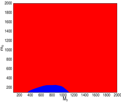
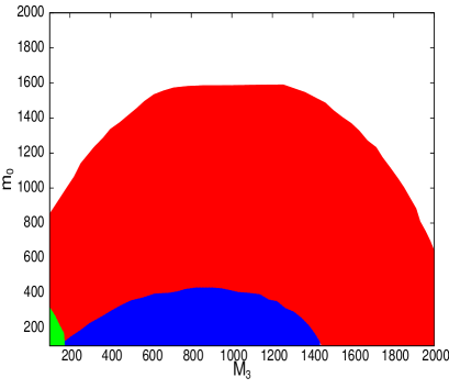
Figure 1: Parameter space scan for the representation 770 (breaking through $G_{422}$) at high scale $M_{3}-m_{0}$ plane (in GeV), showing the regions allowed by various constraints. Figure on the left hand side: $\tan\beta$= 5. The red region is allowed and the blue region at the bottom is disfavoured by stau-LSP. Figure on the right hand side: $\tan\beta$= 40. The region in red is allowed by all constraints. Region in white is disfavoured by REWSB, the low-$m_{0}$ region, in blue, is disfavoured by stau-LSP and the left corner of the graph in green with small $M_{3}$ and $m_{0}$ is disfavoured by $b\rightarrow s\gamma$.

Figure 2, shows similar parameter space scan for the case of mSUGRA, for $\tan\beta$= 5 (left) and $\tan\beta$= 40 (right). These are presented to show the difference in the low-energy parameter space consistency patterns for different high scale gaugino mass inputs. These cases have been studied well and need not require much illustration. Our scan seems to match with the earlier available results [19] and show the robustness of our analysis. However, it is worth mentioning that the red region, excepting for the blue region at small $m_{0}$ (disfavoured by stau-LSP), is allowed for $\tan\beta$= 5. For $\tan\beta$=40, a small region at the upper left corner with high values of $m_{0}$ (1200-2000 GeV) and small $M_{3}$ (100-400 GeV) (in white) is disfavoured by REWSB. The blue region at the bottom is disfavoured for stau-LSP.

      

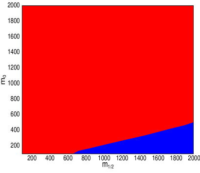
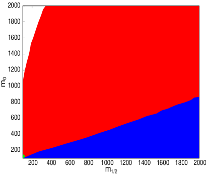
Figure 2: Parameter space scan for mSUGRA at high scale $m_{1/2}-m_{0}$ plane (in GeV), showing the regions allowed by various constraints. Figure on the left side: $\tan\beta$= 5. The red region is allowed. The blue region at the bottom with low $m_{0}$ is disfavoured by stau-LSP. Figure on the right side: $\tan\beta$= 40. The red region is allowed. The region in white at the left corner with high values of $m_{0}$ (1200-2000 GeV) is disallowed by REWSB and the bottom of the figure in blue with low values of $m_{0}$ (100-600 GeV), is disfavoured by stau-LSP.

The benchmark points (BPs) chosen from Figure 1, to study the collider signature in context of the LHC, are presented in Table 3 and 4. In Table 3, we mention the high scale input parameters, while the low-energy spectra corresponding to these points have been mentioned in Table 4. The points have been chosen for two different values of $\tan\beta$, 5 (BP1, BP2, BP3) and 40 (BP4, BP5) and have gluino masses around 500 GeV and 1000 GeV. These points for $\tan\beta$= 5 satisfy the WMAP data for the cold dark matter relic density search, while the points for $\tan\beta$= 40 are all below the lower limit quoted by WMAP. The corresponding values of $\Omega_{CDM}h^{2}$ have also been mentioned in Table 3. These points also obey the LEP bounds [40]. The model under scrutiny has been referred as 770-422 in Table 3 and will be referred so in the following text.

Benchmark Points	Model	$M_{3}$	$m_{0}$	$\tan\beta$	$\Omega_{CDM}h^{2}$
BP1	770-422	200	200	5	0.124
BP2	770-422	400	140	5	0.125
BP3	770-422	600	300	5	0.126
BP4	770-422	200	200	40	0.0002
BP5	770-422	400	700	40	0.0162

Table 3: Benchmark Points (BP): Models, High scale input parameters (in GeV), $\tan\beta$ and $\Omega_{CDM}h^{2}$.

Benchmark Points	$m_{\tilde{g}}$	$m_{\tilde{q}_{1,2}}$	$m_{\tilde{l}_{1,2}}$	$m_{\tilde{\chi}^{0}_{1}}$	$m_{\tilde{\chi}^{\pm}_{1}}$	$\mu$
		$m_{\tilde{t}_{1}}$	$m_{\tilde{\tau}_{1}}$		$m_{\tilde{\chi}^{0}_{2}}$
BP1	499.95	524	319.5	138.43	203.5	221.4
		305.26	246.79		219.56
BP2	938.8	928	495	303.53	375.96	381.18
		551.83	313.93		386.92
BP3	1368.48	1366	770.5	464.3	515.65	515.27
		815.14	513.84		522.39
BP4	499.5	524.5	320	132.23	170.45	178.36
		315	172.25		187.51
BP5	966.58	1145	857	246.73	262.11	261.83
		699.06	597.87		269.58

Table 4 : Low-energy spectra for the chosen benchmark points (BP) (in GeV).

In Table 4, we note the gluino mass ($m_{\tilde{g}}$), average of the first two generation squark masses ($m_{\tilde{q}_{1,2}}$), average of the first two generation slepton masses ($m_{\tilde{l}_{1,2}}$), lighter stau mass ($m_{\tilde{\tau}_{1}}$), lighter stop ($m_{\tilde{t}_{1}}$), lightest neutralino ($m_{\tilde{\chi}^{0}_{1}}$), lighter chargino ($m_{\tilde{\chi}^{\pm}_{1}}$), 2nd lightest neutralino ($m_{\tilde{\chi}^{0}_{2}}$) as well as the value of $\mu$, generated by REWSB at the BPs. It can also be noted that BP1, BP2, BP3 have bino dominated $\tilde{\chi}^{0}_{1}$, while it is mixed and higgsino dominated in case of BP4 and BP5 respectively. The $\tilde{\chi}^{0}_{2}$ is mixed in case of BP1 and higgsino dominated in all the other cases. The lighter chargino is mostly higgsino dominated and degenerate with $\tilde{\chi}^{0}_{2}$, excepting for the case of BP1. We would like to mention that, the composition (gaugino dominated, higgsino dominated or mixed) and the mass difference of the neutralinos and charginos get altered for different high scale gaugino non-universality. Given the similar values of squark and gluino masses in different non-universal schemes (actually similar choices of $M_{3}$ and $m_{0}$ at the high scale), the electroweak gauginos become instrumental for a possible distinction between different GUT-breaking schemes, which might also get reflected at the collider signature in a favourable region of parameter space.

To see such distinction in collider signature, we choose two points from mSUGRA scenario with suitable values of $M_{1/2}$ such that the low scale gluino masses are around 500 GeV and 1000 GeV (similar to the benchmark points (BP) selected above) in a region of parameter space that satisfies the WMAP data for cold dark matter constraint. It should be noted that once these points respect the CDM constraint, the value of $m_{0}$ automatically get restricted for a particular choice of $M_{1/2}$ for a specific $\tan\beta$. Similar is the situation here where we have taken $\tan\beta$ = 5 for illustration. The chosen points are named as MSG1 and MSG2. The high scale parameters along with the $\Omega_{CDM}h^{2}$ at these points are mentioned in Table 5, while the corresponding low scale spectra are noted in Table 6.

Points	Model	$m_{1/2}$	$m_{0}$	$\tan\beta$	$\Omega_{CDM}h^{2}$
MSG1	mSUGRA	480	100	5	0.111
MSG2	mSUGRA	200	70	5	0.128

Table 5: mSUGRA points (MSG): Models, High scale input parameters (in GeV), $\tan\beta$ and $\Omega_{CDM}h^{2}$.

Points	$m_{\tilde{g}}$	$m_{\tilde{q}_{1,2}}$	$m_{\tilde{l}_{1,2}}$	$m_{\tilde{\chi}^{0}_{1}}$	$m_{\tilde{\chi}^{\pm}_{1}}$	$\mu$
		$m_{\tilde{t}_{1}}$	$m_{\tilde{\tau}_{1}}$		$m_{\tilde{\chi}^{0}_{2}}$
MSG1	1104.1	992	272	195.66	367.1	622.1
		768.6	205.1		367.4
MSG2	493.25	452	129	73.2	131.4	281.4
		323.6	101.3		133.6

Table 6 : Low-energy spectra for the chosen mSUGRA points (MSG).

4 Collider Simulation and Numerical Results

We would like to discuss the collider signature now, of the benchmark points advocated in the preceeding section.

We first discuss the strategy for the simulation which includes the final state observables and the cuts employed therein. In the next subsection we discuss the numerical results obtained from this analysis.

4.1 Strategy for Simulation

The spectrum generated by SuSpect v2.3 as described in the earlier section, at the benchmark points are fed into the event generator Pythia 6.4.16 [41] by SLHA interface [42] for the simulation of $pp$ collision with centre of mass energy 14 TeV.

We have used CTEQ5L [43] parton distribution functions, the QCD renormalization and factorization scales being both set at the subprocess centre-of-mass energy $\sqrt{\hat{s}}$. All possible SUSY processes and decay chains consistent with conserved $R$-parity have been kept open. We have kept initial and final state radiations on. The effect of multiple interactions has been neglected. However, we take hadronization into account using the fragmentation functions inbuilt in Pythia.

The final states studied here are :

• Opposite sign dilepton ($OSD$) : $(\ell^{\pm}\ell^{\mp})+(\geq 2)~{}jets~{}+{E_{T}}\!\!\!\!/$

• Same sign dilepton ($SSD$) : $(\ell^{\pm}\ell^{\pm})+(\geq 2)~{}jets~{}+{E_{T}}\!\!\!\!/$

• Trilepton $(3\ell+jets)$: $3\ell~{}+(\geq 2)~{}jets~{}+{E_{T}}\!\!\!\!/$

• Hadronically quiet trilepton $(3\ell)$: $3\ell~{}+(0)~{}jets~{}+{E_{T}}\!\!\!\!/$

• Inclusive 4-lepton ($4\ell$): $4\ell+X+{E_{T}}\!\!\!\!/$

where $\ell$ stands for final state isolated electrons and or muons, ${E_{T}}\!\!\!\!/$ depicts the missing energy, $X$ indicates any associated jet production.

We will discuss these objects in details, that constitute the final state observables. The nomenclature assigned to the final state events in parantheses will be referred in the following text.

As defined in some earlier works [24], the absence of any jets with ${E_{T}}^{jet}~{}\geq~{}100$ GeV qualifies the event as hadronically quiet. This avoids unnecessary removing of events along with jets originating from underlying events, pile up effects and ISR/FSR. The $4\ell$ events have been defined without putting an exclusive jet veto.

Before we mention the selection cuts, we would like to discuss the resolution effects of the detectors, specifically of the ECAL, HCAL and that of the muon chamber, which have been incorporated in our analysis. This is particularly important for reconstructing ${E_{T}}\!\!\!\!/$, which is a key variable for discovering physics beyond the standard model.

All the charged particles with transverse momentum, $p_{T}~{}>$ 0.5 GeV that are produced in a collider, are detected due to strong B-field within a pseudorapidity range $|\eta|<5$, excepting for the muons where the range is $|\eta|<2.5$, due to the characteristics of the muon chamber. Experimentally, the main ’physics objects’ that are reconstructed in a collider, are categorised as follows:

• Isolated leptons identified from electrons and muons

• Hadronic Jets formed after identifying isolated leptons

• Unclustered Energy made of calorimeter clusters with $p_{T}~{}>$ 0.5 GeV (ATLAS) and $|\eta|<5$, not associated to any of the above types of high-$E_{T}$ objects (jets or isolated leptons).

Below we discuss the ’physics objects’ described above in details.

• Isolated leptons ($iso~{}\ell$):

Isolated leptons are identified as electrons and muons with $p_{T}>$ 10 GeV and $|\eta|<$2.5. An isolated lepton should have lepton-lepton separation ${\bigtriangleup R}_{\ell\ell}~{}\geq$0.2, lepton-jet separation (jets with $E_{T}>$ 20 GeV) ${\bigtriangleup R}_{{\ell}j}~{}\geq 0.4$, the energy deposit $\sum{E_{T}}$ due to low-$E_{T}$ hadron activity around a lepton within $\bigtriangleup R~{}\leq 0.2$ of the lepton axis should be $\leq$ 10 GeV, where $\bigtriangleup R=\sqrt{{\bigtriangleup\eta}^{2}+{\bigtriangleup\phi}^{2}}$ is the separation in pseudo rapidity and azimuthal angle plane. The smearing functions of isolated electrons, photons and muons are described below.

• Jets ($jet$):

Jets are formed with all the final state particles after removing the isolated leptons from the list with PYCELL, an inbuilt cluster routine in Pythia. The detector is assumed to stretch within the pseudorapidity range $|\eta|$ from -5 to +5 and is segmented in 100 pseudorapidity ($\eta$) bins and 64 azimuthal ($\phi$) bins. The minimum $E_{T}$ of each cell is considered as 0.5 GeV, while the minimum $E_{T}$ for a cell to act as a jet initiator is taken as 2 GeV. All the partons within $\bigtriangleup R$=0.4 from the jet initiator cell is considered for the jet formation and the minimum $\sum_{parton}{E_{T}}^{jet}$ for a collected cell to be considered as a jet is taken to be 20 GeV. We have used the smearing function and parameters for jets that are used in PYCELL in Pythia.

• Unclustered Objects ($Unc.O$):

Now, as has been mentioned earlier, all the other final state particles, which are not isolated leptons and separated from jets by $\bigtriangleup R\geq$0.4 are considered as unclustered objects. This clearly means all the particles (electron/photon/muon) with $0.5<E_{T}<10$GeV and $|\eta|<5$ (for muon-like track $|\eta|<2.5$) and jets with $0.5<E_{T}<20$GeV and $|\eta|<5$, which are detected at the detector, are considered as unclustered energy and their resolution function have been considered separately and mentioned below.

• Electron/Photon Energy Resolution :

  $$\sigma(E)/E=a/\sqrt{E}\oplus b\oplus c/E$$ (28)

  Where,
           $a$ = 0.03 [GeV^1/2],    $b$ = 0.005 &   $c$ = 0.2 [GeV]     for $|\eta|<1.5$
              = 0.055                  = 0.005         = 0.6           for $1.5<|\eta|<5$
  

• Muon $P_{T}$ Resolution :

  $$\sigma(P_{T})/P_{T} = a~{}~{}~{}~{}~{}~{}~{}~{}~{}~{}~{}~{}~{}~{}~{}~{}~{}~{}~{}~{}~{}~{}~{}{\rm if}~{}P_{T}<100GeV$$ (29)

  $$= a+b\log(P_{T}/\xi)~{}~{}~{}~{}~{}{\rm if}~{}P_{T}>100GeV$$ (30)

  Where,
           $a$= 0.008   & $b$= 0.037       for $|\eta|<1.5$
            = 0.02        = 0.05           $1.5<|\eta|<2.5$

• Jet Energy Resolution :

  $$\sigma(E_{T})/E_{T}=a/\sqrt{E_{T}}$$ (31)

  Where,
           a= 0.55 [GeV^1/2], default value used in PYCELL.

• Unclustered Energy Resolution :

  $$\sigma(E_{T})=\alpha\sqrt{\Sigma_{i}E^{(Unc.O)i}_{T}}$$ (32)

  Where, $\alpha\approx 0.55$. One should keep in mind that the x and y component of $E^{Unc.O}_{T}$ need to be smeared independently with same smearing parameter.

All the smearing parameters that have been used are mostly in agreement with the ATLAS detector specifications and also have been discussed in details in [44]

Once we have identified the ’physics objects’ as described above, we sum vectorially the x and y components of the smeared momenta separately for isolated leptons, jets and unclustered objects in each event to form visible transverse momentum $(p_{T})_{vis}$,

$$(p_{T})_{vis}=\sqrt{(\sum p_{x})^{2}+(\sum p_{y})^{2}}$$ (33)

where, $\sum p_{x}=\sum(p_{x})_{iso~{}\ell}+\sum(p_{x})_{jet}+\sum(p_{x})_{Unc.O}$ and similarly for $\sum p_{y}$. We identify the negative of the $(p_{T})_{vis}$ as missing energy $E_{T}\!\!\!\!/$:

$$E_{T}\!\!\!\!/=-(p_{T})_{vis}$$ (34)

Finally the selection cuts that are used in our analysis are as follows:

• Missing transverse energy $E_{T}\!\!\!\!/$ $\geq~{}100$ GeV.

• ${p_{T}}^{\ell}~{}\geq~{}20$ GeV for all isolated leptons.

• ${E_{T}}^{jet}~{}\geq~{}100$ GeV and $|{\eta}_{jet}|~{}\leq~{}2.5$

• For OSD, hadronically quiet trilepton ($3\ell$) and also for inclusive $4\ell$ events we have used, in addition, invariant mass cut on the same flavour opposite sign lepton pair as $|M_{Z}-M_{\ell_{+}\ell_{-}}|~{}\geq 10$ GeV.

We have checked the hard scattering cross-sections of various production processes with CalcHEP [45]. All the final states with jets at the parton level have been checked against the results available in [27]. The calculation of hadronically quiet trilepton rates have been checked against [46], in the appropriate limits.

We have generated dominant SM events in Pythia for the same final states with same cuts. $t\bar{t}$ production gives the most serious backgrounds. We have multiplied the corresponding events in different channels by proper $K$-factor ($=2.23$) to obtain the usually noted next to leading order (NLO) and next to leading log resummed (NLL) cross-section of $t\bar{t}$ production at the LHC, 908 pb (without taking the PDF and scale uncertainty), for $m_{t}$ around 171 GeV [47]. The other sources of background include $WZ$ production, $ZZ$ production etc. The contribution of each of these processes to the various final states are mentioned in the Table 9.

4.2 Numerical Results

Figure 3 shows the effective mass distribution at the benchmark points and the corresponding mSUGRA ones in $OSD$ events. Effective mass is defined as

$$Effective~{}mass=\sum(p_{T})_{iso~{}\ell}+\sum(p_{T})_{jets}+E_{T}\!\!\!\!/$$ (35)

Figure 3 has been organised following the model inputs. Top left figure shows the distributions at BP1, BP2 and BP3 chosen from 770-422 with $\tan\beta$=5, whereas the top right one contains BP4 and BP5 chosen from the same scenario with $\tan\beta$=40 and the one from $t\bar{t}$ production, the dominant process for the background. The bottom one is for mSUGRA, containing MSG1 and MSG2 with $\tan\beta$=5. The peak of the effective mass distribution corresponds to the threshold energy of the hard scattering process which is dominantly responsible for the final state under scrutiny. For $OSD$ events, processes responsible are mostly the $\tilde{g}\tilde{g}$, $\tilde{g}\tilde{q}$ and $\tilde{q}\tilde{q}$ productions due to their $SU(3)$ interactions, provided they are accessible to the LHC center of mass energy. In such cases, the threshold energy is around $2m_{\tilde{g}}$ or ($m_{\tilde{g}}+m_{\tilde{q}}$) or $2m_{\tilde{q}}$. Now, in each of the BPs advocated here, $m_{\tilde{g}}=m_{\tilde{q}}$ and the threshold is approximately at $2m_{\tilde{g}}$. Our figures magnificently depict the correspondence with such threshold. For example, the peaks of BP1, BP4 and MSG2 are greater than 1000 GeV (where the gluino and squark masses are around 500 GeV). The reason that these distributions peak at higher values than the threshold, can be attributed to the fact that the final state considered here, has a very large $E_{T}\!\!\!\!/$ cut, $(p_{T})$ cut on associated jets and leptons. While this indicates the robustness of our analysis, this also points to the deficiency in distinguishing these non-universal models from the mSUGRA one with similar gluino masses. However, a possible way that could have been exploited is perhaps the effective mass distribution in $3\ell$ events. This is expected as the dominant production process for this final state is $\tilde{\chi_{2}}^{0}$ and $\tilde{\chi_{1}}^{\pm}$ and these electroweak gauginos actually carry the information of different non-universal gaugino mass inputs at the GUT scale. However, this was not very successful in our case due to small event rates.

      

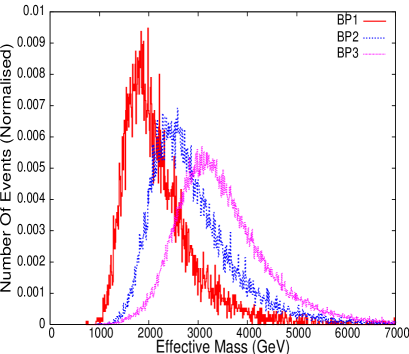
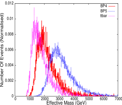
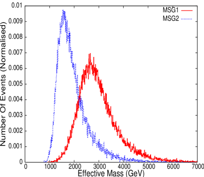
Figure 3: Effective mass distribution in $OSD$ events. Top left: BP1 (Red), BP2 (Blue) and BP3 (Pink) chosen from 770-422 with $\tan\beta$=5 have been plotted. Top right: BP4 (Red) and BP5 (Blue) chosen from 770-422 with $\tan\beta$=40 and $t\bar{t}$ (Pink) have been plotted. Bottom: MSG1 (Red) and MSG2 (Blue) chosen from mSUGRA with $\tan\beta$=5 have been plotted. CTEQ5L pdfset was used. Factorisation and Renormalisation scale has been set to $\mu_{F}=\mu_{R}=\sqrt{\hat{s}}$, sub-process centre of mass energy.

The missing energy distributions in OSD events at all the benchmark points have been shown in Figure 4. The organisation of the points remain the same as in Figure 3. In each case, the distribution starts from 100 GeV, as the event selection itself had this missing energy cut. As a result, all the points show a similar falling feature which indicates that the peak of the distribution is either small or around 100 GeV. The difference in the distributions is in the tail and is due to the hierarchy of the lightest neutralino masses. The heavier is the neutralino, the flatter is the distribution. Although this gives a nice distinction between the points with different gluino masses (and hence with different LSP masses), it is again, difficult to distinguish points with similar gluino masses.

      

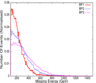
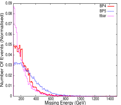
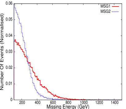
Figure 4: Missing energy distribution in $OSD$ events. Top left: BP1 (Red), BP2 (Blue) and BP3 (Pink) chosen from 770-422 with $\tan\beta$=5 have been plotted. Top right: BP4 (Red) and BP5 (Blue) chosen from 770-422 with $\tan\beta$=40 and $t\bar{t}$ (Pink) have been plotted. Bottom: MSG1 (Red) and MSG2 (Blue) chosen from mSUGRA with $\tan\beta$=5 have been plotted. CTEQ5L pdfset was used. Factorisation and Renormalisation scale has been set to $\mu_{F}=\mu_{R}=\sqrt{\hat{s}}$, sub-process centre of mass energy.

The numerical values of the event rates at the benchmark points are presented in Table 7, while Table 8 contains the results in similar channels for the mSUGRA ones. We note the contributions to these channels from the SM background in Table 9. While we note that the results are widely different from each other for different BPs, we also point out the distinction with corresponding mSUGRA ones with similar gluino masses. For example, when we compare BP1, BP4 and MSG2 (all with gluino masses around 500 GeV), we note that the mSUGRA point yields much more events in almost all channels. This primarily has two reasons: one, the choice of the scalar mass parameter is very low for the mSUGRA one, compared to the non-universal case to obey CDM constraint and two, the non-universal scenario studied here, have higher values of $M_{1}$ and $M_{2}$ at the high scale, which make the low-lying charginos and neutralinos heavier and correspondingly lower decay branching fraction through these to the leptonic final states. Similar observation can be made in an attempt to compare the event rates of BP2, BP3, BP5 and MSG1 ($m_{\tilde{g}}\simeq$ 1000 GeV). The reason that BP2 has slightly higher event rates than MSG1 can be attributed to the fact that $m_{\tilde{g}}$= 938.8 GeV for BP1, which is smaller to be compared to MSG1 ($m_{\tilde{g}}$= 1104 GeV).

While we see that almost all the channels at the BPs rise sufficiently over the background fluctuations, the hadronically quiet trilepton channel gets submerged in to the background even for an integrated luminosity 100$fb^{-1}$ at the points BP2, BP3, BP5 and MSG1. This is because of the very high values of $m_{\tilde{\chi_{2}}^{0}}$ and $m_{\tilde{\chi_{1}}^{\pm}}$ with very small $\Delta m_{(\tilde{\chi_{2}}^{0}/\tilde{\chi_{1}}^{\pm}-\tilde{\chi_{1}}^{0})}$. The significance in most of these points, in most of the channels (excepting the ${3\ell}$), are so high that it is very unlikely to be affected by the systematic errors. We would also like to point out that all the channels in BP1, BP4 and MSG2 rise over the background even for an integrated luminosity of 10$fb^{-1}$ (only exception being the $\sigma_{3\ell}$ for BP4), while others are suppressed by the background. In Table 10, we summarise this information for each of the channels and parameter points, for an integrated luminosity of 30$fb^{-1}$.

In the tables, the cross-sections are named as follows: $\sigma_{OSD}$ for OSD, $\sigma_{SSD}$ for SSD, $\sigma_{3\ell+jets}$ for $(3\ell+jets)$, $\sigma_{3\ell}$ for $(3\ell)$ and $\sigma_{4\ell}$ for inclusive 4 lepton events $4\ell$.

Benchmark Points	$\sigma_{OSD}$	$\sigma_{SSD}$	$\sigma_{3\ell+jets}$	$\sigma_{3\ell}$	$\sigma_{4\ell}$
BP1	597.7	102.9	57.6	13.10	10.30
BP2	70.1	15.7	11.6	0.09	1.64
BP3	17.9	2.2	4.0	0.01	1.16
BP4	398.4	120.8	30.8	4.50	3.28
BP5	26.5	12.2	3.9	0.05	0.33

Table 7: Event-rates (fb) in multilepton channels at the chosen benchmark points. CTEQ5L pdfset was used. Factorisation and Renormalisation scale has been set to $\mu_{F}=\mu_{R}=\sqrt{\hat{s}}$, subprocess centre of mass energy.

mSUGRA Points	$\sigma_{OSD}$	$\sigma_{SSD}$	$\sigma_{3\ell+jets}$	$\sigma_{3\ell}$	$\sigma_{4\ell}$
MSG1	50.9	16.4	10.6	0.08	1.34
MSG2	2781.8	175.9	285.1	12.26	99.89

Table 8: Event-rates (fb) in multilepton channels at the mSUGRA points. CTEQ5L pdfset was used. Factorisation and Renormalisation scale has been set to $\mu_{F}=\mu_{R}=\sqrt{\hat{s}}$, subprocess centre of mass energy.

SM Processes	$\sigma_{OSD}$	$\sigma_{SSD}$	$\sigma_{3\ell+jets}$	$\sigma_{3\ell}$	$\sigma_{4\ell}$
$t\bar{t}$	1102	18.1	2.7	5.3	0.0
$ZZ$,$WZ$,$ZH$,$Z\gamma$	16.3	0.3	0.5	1.1	0.4
Total	1118.3	18.4	3.2	6.4	0.4

Table 9: Event-rates after cut (fb) in multilepton channels from the dominant SM backgrounds. The event rates in different channels for $t\bar{t}$ production have been multiplied by by proper $K$-factor (2.23) to obtain the usually noted NLO+NLL cross-section of $t\bar{t}$ [47]. CTEQ5L pdfset was used. Factorisation and Renormalisation scale has been set to $\mu_{F}=\mu_{R}=\sqrt{\hat{s}}$, subprocess centre of mass energy.

Model Points	${OSD}$	${SSD}$	${3\ell+jets}$	${3\ell}$	${4\ell}$
BP1	$\surd$	$\surd$	$\surd$	$\surd$	$\surd$
BP2	$\surd$	$\surd$	$\surd$	$\times$	$\surd$
BP3	$\times$	$\times$	$\surd$	$\times$	$\surd$
BP4	$\surd$	$\surd$	$\surd$	$\surd$	$\surd$
BP5	$\surd$	$\surd$	$\surd$	$\times$	$\times$
MSG1	$\surd$	$\surd$	$\surd$	$\times$	$\surd$
MSG2	$\surd$	$\surd$	$\surd$	$\surd$	$\surd$

Table 10 : $5\sigma$ visibility of various signals for an integrated luminosity of $30fb^{-1}$. A $\surd$ indicates a positive conclusion while a $\times$ indicates a negative one.

We also compare these results in the ratio space of events which is demonstrated in Figure 5 in form of barplot. The advantage of going to the ratio space is the uncertainties due to the choice of pdfsets, jet energy scale get reduced. Here we take the ratios of all events with respect to the OSD and referred as SSD/OSD, 3L+JETS/OSD, 3L/OSD and 4L/OSD along the x-axis of the barplot. As earlier, we divide the BPs and the MSGs in two categories: one, with BP1, BP4 and MSG2 ($m_{\tilde{g}}\simeq$ 500 GeV), which is shown in the left panel of the Figure 5; two, BP2, BP3, BP5 and MSG1 ($m_{\tilde{g}}\simeq$ 1000 GeV), which is shown in the right panel of the Figure 5. We note that BP1, BP4 and MSG2 are well distinguished from SSD/OSD, 3L/OSD and 4L/OSD. While BP2 and MSG1 can not be distinguished very well from each other, identification of BP3, BP5 and MSG1 is quite apparent from SSD/OSD and 4L/OSD events.

In a nutshell we can summarise that, it is indeed possible to distinguish the non-universal gaugino mass scenario advocated here, from the mSUGRA ones with similar gluino masses. This is possible in both the absolute event rates or from the ratio plots shown here. However, the distinguishability reduces with increasing gluino mass.

      

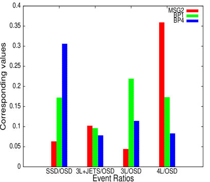
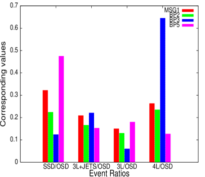
Figure 5: Event ratios of different benchmark points compared with mSUGRA. Along the x-axis, ratios of events with respect to $OSD$ have been taken. The relative values of these ratios for different benchmark points are indicated along the y-axis. Figure on the left: MSG2 (Red), BP1 (Green) and BP4 (Blue) are compared. $m_{\tilde{g}}$ is around 500 GeV in each case. 3L/OSD and 4L/OSD have been multiplied by 10. Figure on the right: MSG1 (Red), BP2 (Green), BP3 (Blue) and BP5 (Pink) are compared. $m_{\tilde{g}}$ is around 1000 GeV in each case. 3L/OSD has been multiplied by 100 and 4L/OSD has been multiplied by 10 to accommodate them in the same figure. CTEQ5L pdfset was used. Factorisation and Renormalisation scale has been set to $\mu_{F}=\mu_{R}=\sqrt{\hat{s}}$, sub-process centre of mass energy.

5 Summary and Conclusions

We have derived non-universal gaugino mass ratios for the representations 54 and 770 for the breaking chain $SU(4)_{C}\times SU(2)_{L}\times SU(2)_{R}~{}(G_{422})$ in a $SO(10)$ SUSY-GUT scenario. We have assumed that the breaking of $SO(10)$ to the intermediate gauge group and the latter in turn to the SM gauge group takes place at the GUT scale itself. We point out some errors in the earlier calculation and derive new results on the gaugino mass ratios. We scan the parameter space with different low-energy constraints taken into account and point out the allowed region of the parameter space. We also study the dark matter constraint in these models and study collider simulation at some selected benchmark points in context of the LHC. The scans presented, have many interesting features that might help us in understanding the correlation between high scale input and low-energy spectra. We must mention here that the study is limited by the assumption that the series of symmetry breaking occurs at the GUT scale itself. It is essentially a simplification, although we know that the mass relation in Equation (22) is not going to change with different choices of the intermediate scale, while the running of the masses from the GUT scale to the intermediate scale will eventually change the gaugino mass ratios. However, our choice of the non-singlet Higgses, apart from conserving $D$-parity, are compatible even if the intermediate scale is different from the GUT scale. Within such a framework we have performed a collider study which is more illustrative than exhaustive. It nonetheless elicits some characteristics of the signature space for such high scale ratios in context of the LHC. It is worth mentioning in this context that the comparison between the non-universal inputs with the mSUGRA ones yields a significant distinction in the multilepton channel parameter space in context of the LHC. This feature might be important in pointing out the departure of the ’signature space’ with the inclusion of non-universality at the high scale.

While this paper was in preparation, we came across the reference [48], where the issue of gaugino mass non-universality in the context of $SO(10)$ and $E(6)$ has been addressed. While we agree completely with the corrected gaugino mass ratios for $G_{422}$, our analysis in addition, point out the phenomenologically viable situations where the choices of the Higgses get restricted with $D$-parity conservation and inclusion of the intermediate scale different from the GUT scale. Furthermore, the low-energy particle spectra in different cases have been derived in a comparative manner and the allowed regions of the parameter space consistent with low-energy and dark matter constraints are obtained in each case. In addition, we have predicted event-rates for such a breaking chain in a multichannel study pertinent to the LHC. The distinguishability of relative rates in different channels has also been explicitly demonstrated by us.

Acknowledgment:

We thank Biswarup Mukhopadhyaya and Amitava Raychaudhuri for many useful suggestions. We thank Sanjoy Biswas, Debottam Das and Nishita Desai for their technical help. We also acknowledge some very helpful comments from AseshKrishna Datta and Sourav Roy. This work was partially supported by funding available from the Department of Atomic Energy, Government of India for the Regional Centre for Accelerator-based Particle Physics, Harish-Chandra Research Institute. Computational work for this study was partially carried out at the cluster computing facility of Harish-Chandra Research Institute (http://cluster.mri.ernet.in).

Appendix

Using Equation (15) in Section 2, $T_{Y}$, $T_{B-L}$ and $T_{3R}$ in 45-dimension can be written as:

$$T_{Y}=\sqrt{\frac{3}{5}}diag(\underbrace{0,..0}_{8},\frac{2}{3},\frac{2}{3},\frac{2}{3},-\frac{2}{3},-\frac{2}{3},-\frac{2}{3},\underbrace{0,..0}_{4},1,0,-1,\underbrace{\frac{1}{6},..,\frac{1}{6}}_{6},\underbrace{-\frac{5}{6},..,-\frac{5}{6}}_{6},\underbrace{\frac{5}{6},..,\frac{5}{6}}_{6},\underbrace{-\frac{1}{6},..,-\frac{1}{6}}_{6})$$ (36)

$$T_{B-L}=\sqrt{\frac{3}{8}}diag(\underbrace{0,..0}_{8},\frac{4}{3},\frac{4}{3},\frac{4}{3},-\frac{4}{3},-\frac{4}{3},-\frac{4}{3},\underbrace{0,..0}_{6},\underbrace{-\frac{2}{3},..,-\frac{2}{3}}_{12},\underbrace{\frac{2}{3},..,\frac{2}{3}}_{12})$$ (37)

$$T_{3R}=diag(\underbrace{0,..0}_{15},\underbrace{0,..0}_{3},1,0,-1,\underbrace{\frac{1}{2},..,\frac{1}{2}}_{6},\underbrace{-\frac{1}{2},..,-\frac{1}{2}}_{6},\underbrace{\frac{1}{2},..,\frac{1}{2}}_{6},\underbrace{-\frac{1}{2},..,-\frac{1}{2}}_{6})$$ (38)

These lead to the following relation

$$T_{Y}=\sqrt{\frac{3}{5}}T_{3R}+\sqrt{\frac{2}{5}}T_{B-L}$$ (39)

References

- [1] For reviews see for example, H. E. Haber and G. L. Kane, “The Search For Supersymmetry: Probing Physics Beyond The Standard Model,” Phys. Rept. 117, 75 (1985).
- [2] S. Dawson, E. Eichten and C. Quigg, “Search For Supersymmetric Particles In Hadron - Hadron Collisions,” Phys. Rev. D 31, 1581 (1985); X. Tata, “What is supersymmetry and how do we find it?,” arXiv:hep-ph/9706307.
- [3] A. V. Gladyshev and D. I. Kazakov, “Supersymmetry and LHC,” arXiv:hep-ph/0606288.
- [4] S. P. Martin, “A supersymmetry primer,” arXiv:hep-ph/9709356 and in G. Kane (ed), Perspectives On Supersymmetry, World Scientific (1998); M. E. Peskin, “Supersymmetry in Elementary Particle Physics,” arXiv:0801.1928 [hep-ph].
- [5] T. Moroi and L. Randall, “Wino cold dark matter from anomaly-mediated SUSY breaking,” Nucl. Phys. B 570 (2000) 455 [arXiv:hep-ph/9906527]; M. E. Gomez and J. D. Vergados, “Cold dark matter detection in SUSY models at large tan(beta),” Phys. Lett. B 512 (2001) 252 [arXiv:hep-ph/0012020].
- [6] P. Langacker, “Grand Unified Theories And Proton Decay,” Phys. Rept. 72 (1981) 185. D. V. Nanopoulos and K. Tamvakis, “Susy Guts: 4 - Guts: 3,” Phys. Lett. B 113 (1982) 151; J. R. Ellis, D. V. Nanopoulos and S. Rudaz, “Guts 3: Susy Guts 2,” Nucl. Phys. B 202 (1982) 43; L. E. Ibanez and G. G. Ross, “SU(2)-L X U(1) Symmetry Breaking As A Radiative Effect Of Supersymmetry Breaking In Guts,” Phys. Lett. B 110 (1982) 215; N. Polonsky and A. Pomarol, “GUT effects in the soft supersymmetry breaking terms,” Phys. Rev. Lett. 73 (1994) 2292 [arXiv:hep-ph/9406224].
- [7] A. A. Anselm and A. A. Johansen, “Susy GUT With Automatic Doublet - Triplet Hierarchy,” Phys. Lett. B 200 (1988) 331; R. Hempfling, “Neutrino Masses and Mixing Angles in SUSY-GUT Theories with explicit R-Parity Breaking,” Nucl. Phys. B 478 (1996) 3 [arXiv:hep-ph/9511288].
- [8] L. Alvarez-Gaume, J. Polchinski and M. B. Wise, “Minimal Low-Energy Supergravity,” Nucl. Phys. B 221 (1983) 495; A. H. Chamseddine, R. Arnowitt and P. Nath, “Locally Supersymmetric Grand Unification,” Phys. Rev. Lett. 49, 970 (1982).
- [9] J. R. Ellis, C. Kounnas and D. V. Nanopoulos, “No Scale Supersymmetric Guts,” Nucl. Phys. B 247, 373 (1984); J. R. Ellis, K. Enqvist, D. V. Nanopoulos and K. Tamvakis, “Gaugino Masses And Grand Unification,” Phys. Lett. B 155, 381 (1985).
- [10] M. Drees, “Phenomenological Consequences Of N=1 Supergravity Theories With Nonminimal Kinetic Energy Terms For Vector Superfields,” Phys. Lett. B 158, 409 (1985).
- [11] A. Corsetti and P. Nath, “Gaugino mass nonuniversality and dark matter in SUGRA, strings and D brane models,” Phys. Rev. D 64, 125010 (2001) [arXiv:hep-ph/0003186].
- [12] N. Chamoun, C. S. Huang, C. Liu and X. H. Wu, “Non-universal gaugino masses in supersymmetric SO(10),” Nucl. Phys. B 624, 81 (2002) [arXiv:hep-ph/0110332].
- [13] J. Chakrabortty and A. Raychaudhuri, “A note on dimension-5 operators in GUTs and their impact,” Phys. Lett. B 673 (2009) 57 [arXiv:0812.2783 [hep-ph]].
- [14] D. Chang, R. N. Mohapatra and M. K. Parida, “Decoupling Parity And SU(2)-R Breaking Scales: A New Approach To Left-Right Symmetric Models,” Phys. Rev. Lett. 52 (1984) 1072.
- [15] E. Komatsu et al. [WMAP Collaboration], “Five-Year Wilkinson Microwave Anisotropy Probe Observations:Cosmological Interpretation,” arXiv:0803.0547 [astro-ph].
- [16] A. Datta, A. Datta and M. K. Parida, “Signatures of non-universal soft breaking sfermion masses at hadron colliders,” Phys. Lett. B 431, 347 (1998) [arXiv:hep-ph/9801242]; A. Datta, A. Datta, M. Drees and D. P. Roy, “Effects of SO(10) D-terms on SUSY signals at the Tevatron,” Phys. Rev. D 61, 055003 (2000) [arXiv:hep-ph/9907444].
- [17] H. Baer, C. h. Chen, F. Paige and X. Tata, “Signals for Minimal Supergravity at the CERN Large Hadron Collider II: Multilepton Channels,” Phys. Rev. D 53, 6241 (1996) [arXiv:hep-ph/9512383].
- [18] S. Khalil, “Non universal gaugino phases and the LSP relic density,” Phys. Lett. B 484, 98 (2000) [arXiv:hep-ph/9910408]; S. Komine and M. Yamaguchi, “No-scale scenario with non-universal gaugino masses,” Phys. Rev. D 63, 035005 (2001) [arXiv:hep-ph/0007327].
- [19] K. Huitu, Y. Kawamura, T. Kobayashi and K. Puolamaki, “Phenomenological constraints on SUSY SU(5) GUTs with non-universal gaugino masses,” Phys. Rev. D 61, 035001 (2000) [arXiv:hep-ph/9903528]; K. Huitu, J. Laamanen, P. N. Pandita and S. Roy, “Phenomenology of non-universal gaugino masses in supersymmetric grand unified theories,” Phys. Rev. D 72, 055013 (2005) [arXiv:hep-ph/0502100]; U. Chattopadhyay, D. Das and D. P. Roy, “Mixed Neutralino Dark Matter in Nonuniversal Gaugino Mass Models,” arXiv:0902.4568 [hep-ph].
- [20] K. Choi and H. P. Nilles, “The gaugino code,” JHEP 0704, 006 (2007) [arXiv:hep-ph/0702146].
- [21] S. F. King, J. P. Roberts and D. P. Roy, “Natural Dark Matter in SUSY GUTs with Non-universal Gaugino Masses,” JHEP 0710 (2007) 106 [arXiv:0705.4219 [hep-ph]]; K. Huitu, R. Kinnunen, J. Laamanen, S. Lehti, S. Roy and T. Salminen, “Search for Higgs Bosons in SUSY Cascades in CMS and Dark Matter with Non-universal Gaugino Masses,” Eur. Phys. J. C 58 (2008) 591 [arXiv:0808.3094 [hep-ph]].
- [22] K. Huitu and J. Laamanen, “Relic density in non-universal gaugino mass models with SO(10) GUT symmetry,” arXiv:0901.0668 [hep-ph].
- [23] S. I. Bityukov and N. V. Krasnikov, “Search for SUSY at LHC in jets + E(T)(miss) final states for the case of nonuniversal gaugino masses,” Phys. Lett. B 469, 149 (1999) [Phys. Atom. Nucl. 64, 1315 (2001 YAFIA,64,1391-1398.2001)] [arXiv:hep-ph/9907257]; G. Anderson, H. Baer, C. h. Chen and X. Tata, “The reach of Fermilab Tevatron upgrades for SU(5) supergravity models with non-universal gaugino masses,” Phys. Rev. D 61, 095005 (2000) [arXiv:hep-ph/9903370]; S. I. Bityukov and N. V. Krasnikov, “The LHC (CMS) discovery potential for models with effective supersymmetry and nonuniversal gaugino masses,” Phys. Atom. Nucl. 65, 1341 (2002) [Yad. Fiz. 65, 1374 (2002)] [arXiv:hep-ph/0102179].
- [24] S. Bhattacharya, A. Datta and B. Mukhopadhyaya, “Non-universal gaugino masses: a signal-based analysis for the Large Hadron Collider,” JHEP 0710 (2007) 080 [arXiv:0708.2427 [hep-ph]]; S. Bhattacharya, A. Datta and B. Mukhopadhyaya, “Non-universal gaugino and scalar masses, hadronically quiet trileptons and the Large Hadron Collider,” Phys. Rev. D 78 (2008) 115018 [arXiv:0809.2012 [hep-ph]].
- [25] P. Bandyopadhyay, A. Datta and B. Mukhopadhyaya, “Signatures of gaugino mass non-universality in cascade Higgs production at the LHC,” Phys. Lett. B 670 (2008) 5 [arXiv:0806.2367 [hep-ph]]; P. Bandyopadhyay, “Probing non-universal gaugino masses via Higgs boson production under SUSY cascades at the LHC: A detailed study,” arXiv:0811.2537 [hep-ph].
- [26] A. A. Affolder et al. [CDF Collaboration], “Search for gluinos and scalar quarks in collisions at TeV using the missing energy plus multijets signature,” Phys. Rev. Lett. 88, 041801 (2002) [arXiv:hep-ex/0106001]; P. Binetruy, G. L. Kane, B. D. Nelson, L. T. Wang and T. T. Wang, “Relating incomplete data and incomplete theory,” Phys. Rev. D 70, 095006 (2004) [arXiv:hep-ph/0312248]; J. L. Bourjaily, G. L. Kane, P. Kumar and T. T. Wang, “Outside the mSUGRA box,” arXiv:hep-ph/0504170; G. L. Kane, P. Kumar, D. E. Morrissey and M. Toharia, “Connecting (supersymmetry) LHC measurements with high scale theories,” Phys. Rev. D 75, 115018 (2007) [arXiv:hep-ph/0612287].
- [27] A. Datta, G. L. Kane and M. Toharia, “Is it SUSY?,” arXiv:hep-ph/0510204.
- [28] V. D. Barger, W. Y. Keung and R. J. N. Phillips, “Dimuons From Gauge Fermions Produced In P Anti-P Collisions,” Phys. Rev. Lett. 55, 166 (1985); H. Baer, X. Tata and J. Woodside, “Gluino Cascade Decay Signatures At The Tevatron Collider,” Phys. Rev. D 41, 906 (1990); H. Baer, X. Tata and J. Woodside, “Multi - lepton signals from supersymmetry at hadron super colliders,” Phys. Rev. D 45, 142 (1992); R. M. Barnett, J. F. Gunion and H. E. Haber, “Discovering supersymmetry with like sign dileptons,” Phys. Lett. B 315, 349 (1993) [arXiv:hep-ph/9306204]; A. Datta, K. Kong and K. T. Matchev, “Discrimination of supersymmetry and universal extra dimensions at hadron colliders,” Phys. Rev. D 72, 096006 (2005) [Erratum-ibid. D 72, 119901 (2005)] [arXiv:hep-ph/0509246].
- [29] G. Duckeck et al. [ATLAS Collaboration]. “ATLAS computing: Technical design report.”
- [30] E. Cremmer, B. Julia, J. Scherk, P. van Nieuwenhuizen, S. Ferrara and L. Girardello, “Superhiggs Effect In Supergravity With General Scalar Interactions,” Phys. Lett. B 79, 231 (1978); E. Cremmer, B. Julia, J. Scherk, S. Ferrara, L. Girardello and P. van Nieuwenhuizen, “Spontaneous Symmetry Breaking And Higgs Effect In Supergravity Without Cosmological Constant,” Nucl. Phys. B 147, 105 (1979); E. Cremmer, S. Ferrara, L. Girardello and A. Van Proeyen, “Coupling Supersymmetric Yang-Mills Theories To Supergravity,” Phys. Lett. B 116, 231 (1982); E. Cremmer, S. Ferrara, L. Girardello and A. Van Proeyen, “Yang-Mills Theories With Local Supersymmetry: Lagrangian, Transformation Laws And Superhiggs Effect,” Nucl. Phys. B 212, 413 (1983).
- [31] C. T. Hill, “Are There Significant Gravitational Corrections To The Unification Scale?,” Phys. Lett. B 135, 47 (1984).
- [32] Q. Shafi and C. Wetterich, “Modification Of GUT Predictions In The Presence Of Spontaneous Compactification,” Phys. Rev. Lett. 52, 875 (1984).
- [33] R. Slansky, “Group Theory For Unified Model Building,” Phys. Rept. 79 (1981) 1.
- [34] S. P. Martin and P. Ramond, “Sparticle spectrum constraints,” Phys. Rev. D 48, 5365 (1993) [arXiv:hep-ph/9306314].
- [35] D. M. Pierce, J. A. Bagger, K. T. Matchev and R. j. Zhang, “Precision corrections in the minimal supersymmetric standard model,” Nucl. Phys. B 491 (1997) 3 [arXiv:hep-ph/9606211].
- [36] A. Djouadi, J. L. Kneur and G. Moultaka, “SuSpect: A Fortran code for the supersymmetric and Higgs particle spectrum in the MSSM,” Comput. Phys. Commun. 176, 426 (2007) [arXiv:hep-ph/0211331].
- [37] S. Chen, et al., CLEO Collaboration, Phys. Rev. Lett. 87, 251807 (2001), hep-ex/0108032; P. Koppenburg et al. [Belle Collaboration], “An inclusive measurement of the photon energy spectrum in b –¿ s gamma decays,” Phys. Rev. Lett. 93, 061803 (2004); B. Aubert, et al., BaBar Collaboration, hep-ex/0207076.
- [38] G. Belanger, F. Boudjema, A. Pukhov and A. Semenov, “micrOMEGAs2.0: A program to calculate the relic density of dark matter in a generic model,” Comput. Phys. Commun. 176, 367 (2007) [arXiv:hep-ph/0607059].
- [39] H. Baer, A. Mustafayev, H. Summy and X. Tata, “Mixed Higgsino Dark Matter from a Large SU(2) Gaugino Mass,” JHEP 0710 (2007) 088 [arXiv:0708.4003 [hep-ph]].
- [40] W. M. Yao et al. [Particle Data Group], “Review of particle physics,” J. Phys. G 33, 1 (2006).
- [41] T. Sjostrand, S. Mrenna and P. Skands, “PYTHIA 6.4 physics and manual,” JHEP 0605, 026 (2006) [arXiv:hep-ph/0603175].
- [42] P. Skands et al., “SUSY Les Houches accord: Interfacing SUSY spectrum calculators, decay packages, and event generators,” JHEP 0407, 036 (2004) [arXiv:hep-ph/0311123].
- [43] H. L. Lai et al. [CTEQ Collaboration], “Global QCD analysis of parton structure of the nucleon: CTEQ5 parton distributions,” Eur. Phys. J. C 12, 375 (2000) [arXiv:hep-ph/9903282].
- [44] S. Biswas and B. Mukhopadhyaya, “Neutralino reconstruction in supersymmetry with long-lived staus,” arXiv:0902.4349 [hep-ph].
- [45] A. Pukhov, “CalcHEP 3.2: MSSM, structure functions, event generation, batchs, and generation of matrix elements for other packages,” arXiv:hep-ph/0412191.
- [46] H. Baer, C. H. Chen, F. Paige and X. Tata, “Trileptons from chargino - neutralino production at the CERN Large Hadron Collider,” Phys. Rev. D 50 (1994) 4508 [arXiv:hep-ph/9404212].
- [47] S. Moch and P. Uwer, “Theoretical status and prospects for top-quark pair production at hadron colliders,” Phys. Rev. D 78 (2008) 034003 [arXiv:0804.1476 [hep-ph]].
- [48] S. P. Martin, “Non-universal gaugino masses from non-singlet F-terms in non-minimal unified models,” arXiv:0903.3568 [hep-ph].