Total Variation Restoration of Speckled Images
Using a Split-Bregman Algorithm

Abstract

Multiplicative noise models occur in the study of several coherent imaging systems, such as synthetic aperture radar and sonar, and ultrasound and laser imaging. This type of noise is also commonly referred to as speckle. Multiplicative noise introduces two additional layers of difficulties with respect to the popular Gaussian additive noise model: (1) the noise is multiplied by (rather than added to) the original image, and (2) the noise is not Gaussian, with Rayleigh and Gamma being commonly used densities. These two features of the multiplicative noise model preclude the direct application of state-of-the-art restoration methods, such as those based on the combination of total variation or wavelet-based regularization with a quadratic observation term. In this paper, we tackle these difficulties by: (1) using the common trick of converting the multiplicative model into an additive one by taking logarithms, and (2) adopting the recently proposed split Bregman approach to estimate the underlying image under total variation regularization. This approach is based on formulating a constrained problem equivalent to the original unconstrained one, which is then solved using Bregman iterations (equivalently, an augmented Lagrangian method). A set of experiments show that the proposed method yields state-of-the-art results.

Index Terms—  Speckle, multiplicative noise, total variation, Bregman iterations, augmented Lagrangian, synthetic aperture radar.

1 Introduction

1.1 Coherent Imaging and Speckle Noise

The standard statistical models of coherent imaging systems, such as synthetic aperture radar/sonar (SAR/SAS), ultrasound imaging, and laser imaging, are supported on multiplicative noise mechanisms. With respect to a given resolution cell of the imaging device, a coherent system acquires the so-called in-phase and quadrature components which are collected in a complex reflectivity (with the in-phase and quadrature components corresponding to the real and imaginary parts, respectively). The complex reflectivity of a given resolution cell results from the contributions of all the individual scatterers present in that cell, which interfere in a destructive or constructive manner, according to their spatial configuration. When this configuration is random, it yields random fluctuations of the complex reflectivity, a phenomenon which is termed speckle. The statistical properties of speckle have been widely studied and there is a large body of literature [11], [14]. Assuming no strong specular reflectors and a large number of randomly distributed scatterers in each resolution cell (relative to the carrier wavelength), the squared amplitude (intensity) of the complex reflectivity is exponentially distributed [14]. The term multiplicative noise is clear from the following observation: an exponential random variable can be written as the product of its mean value (parameter of interest) by an exponential variable of unit mean (noise). The scenario just described, known as fully developed speckle, leads to observed intensity images with a characteristic granular appearance due to the very low signal to noise ratio (SNR). Notice that the SNR, defined as the ratio between the squared intensity mean and the intensity variance, is equal to one ($0\,$dB).

1.2 Restoration of Speckled Images: Previous Work

A common approach to improving the SNR in coherent imaging consists in averaging independent observations of the same pixel. In SAR/SAS systems, this procedure is called multi-look ($M$-look, in the case of $M$ looks), and each independent observation may be obtained by a different segment of the sensor array. For fully developed speckle, the SNR of an $M$-look image is $M$. Another way to obtain an M-look image is to low pass filter (with a moving average kernel with support size $M$) a 1-look fully developed speckle image, making evident the tradeoff between SNR and spatial resolution. A great deal of research has been devoted to developing nonuniform filters which average large numbers of pixels in homogeneous regions yet avoid smoothing across discontinuities in order to preserve image detail/edges [9]. Many other speckle reduction techniques have been proposed; see [14] for a comprehensive literature review up to 1998.

A common assumption is that the underlying reflectivity image is piecewise smooth. In image restoration under multiplicative noise, this assumption has been formalized using Markov random fields, under the Bayesian framework [14], [2] and, more recently, using total variation (TV) regularization [1], [12], [16], [17].

1.3 Contribution

In this paper, we adopt TV regularization. In comparison with the canonical additive Gaussian noise model, we face two difficulties: the noise is multiplicative; the noise is non-Gaussian, but follows Rayleigh or Gamma distributions. We tackle these difficulties by first converting the multiplicative model into an additive one (which is a common procedure) and then adopting the recently proposed split Bregman approach to solve the optimization problem that results from adopting a total variation regularization criterion.

Other works that have very recently addressed the restoration of speckled images using TV regularization include [1], [12], [16], [17]. The commonalities and differences between our approach and the ones followed in those papers will be discussed after the detailed description of our method, since this discussion requires notation and concepts which will be introduced in the next section.

2 Problem Formulation

Let ${\bf y}\in\mathbb{R}_{+}^{n}$ denote an $n$-pixels observed image, assumed to be a sample of a random image ${\bf Y}$, the mean of which is the underlying reflectivity image ${\bf x}\in\mathbb{R}_{+}^{n}$, i.e., $\mathbb{E}[{\bf Y}]={\bf x}$. Adopting a conditionally independent multiplicative noise model, we have

$$Y_{i}=x_{i}N_{i},\;\;\mbox{for\ $\;i=1,...,n$,}$$ (1)

where ${\bf N}\in\mathbb{R}_{+}^{n}$ is an image of independent and identically distributed (iid) noise random variables with unit mean, $\mathbb{E}(N_{i})=1$, following a common density $p_{N}$. For $M$-look fully developed speckle noise, $p_{N}$ is a Gamma density with $E[N]=1$, and $\sigma_{N}^{2}=1/M$, i.e.,

$$p_{N}(n)=\frac{M^{M}}{\Gamma(M)}\;n^{M-1}e^{-nM}.$$ (2)

An additive noise model is obtained by taking logarithms of (1). For some pixel of the image, the observation model becomes

$$\underbrace{\log Y}_{G}=\underbrace{\log x}_{z}+\underbrace{\log N}_{W}.$$ (3)

The density of the random variable $W=\log N$ is

$$p_{W}(w)=p_{N}(n=e^{w})\,e^{w}=\frac{M^{M}}{\Gamma(M)}\;e^{Mw}e^{-e^{w}M},$$ (4)

thus

$$p_{G|Z}(g|z)=p_{W}(g-z).$$ (5)

Under the regularization and Bayesian frameworks, the original image is inferred by solving a minimization problem with the form

$$\widehat{{\bf z}}\in\arg\min_{{\bf z}}L({\bf z}),$$ (6)

where $L({\bf z})$ is the penalized minus log-likelihood,

$$L({\bf z}) = -\log p_{{\bf G}|{\bf Z}}({\bf g}|{\bf z})+\lambda\,\phi({\bf z}).$$ (7)

$$= M\sum_{s=1}^{n}\left(z_{s}+e^{g_{s}-z_{s}}\right)+\lambda\,\phi({\bf z})+A,$$ (8)

with $A$ an irrelevant additive constant, $\phi$ the penalty/regularizer (negative of the log-prior, from a the Bayesian perspective), and $\lambda$ the regularization parameter.

In this work, we adopt the TV regularizer, that is,

$$\phi({\bf z})=\mbox{TV}({\bf z})=\sum_{s=1}^{n}\sqrt{(\Delta^{h}_{s}{\bf z})^{2}+(\Delta^{v}_{s}{\bf z})^{2}},$$ (9)

where $(\Delta^{h}_{s}{\bf z}$ and $\Delta^{v}_{s}{\bf z})$ denote the horizontal and vertical first order differences at pixel $s\in\{1,\dots,n\}$, respectively.

Each term $\left(z_{s}+e^{g_{s}-z_{s}}\right)$ of (8), corresponding to the negative log-likelihood, is strictly convex and coercive, thus so is their sum. Since the TV regularizer is also convex (though not strictly so), the objective function $L$ possesses a unique minimizer [6]. In terms of optimization, these are desirable properties that would not hold if we had formulated the inference in the original variables ${\bf x}$, since the resulting negative log-likelihood is not convex; this was the approach followed in [1] and [16].

3 Bregman/Augmented Lagrangian Approach

There are several efficient algorithms to compute the TV regularized solution for a quadratic data term; for recent work, see [3], [5], [8], [10], [19], [21], and other references therein. When the data term is not quadratic, as in (8), the problem is more difficult and far less studied. Herein, we follow the split Bregman approach [10] which is composed of the following two steps: (splitting) a constrained problem equivalent to the original unconstrained one is formulated; (Bregman) this constrained problem is solved using the Bregman iterative approach [20]. Before describing these two steps in detail, we briefly review the Bregman iterative approach. The reader is referred to [10], [20], for more details.

3.1 Bregman Iterations

Consider a constrained optimization problem of the form

$$\min_{\bf x} E({\bf x})$$

s.t. $$H({\bf x})=0,$$ (10)

with $E$ and $H$ convex, $H$ differentiable, and $\min_{\bf x}H({\bf x})=0$ . The so-called Bregman divergence associated with the convex function $E$ is defined as

$$D_{E}^{\mathbf{p}}(\mathbf{x},\mathbf{y})\equiv E(\mathbf{x})-E(\mathbf{y})-\langle\mathbf{p},\mathbf{x}-\mathbf{y}\rangle,$$ (11)

where $\mathbf{p}$ belongs to the subgradient of $E$ at ${\bf y}$, i.e.,

$$\mathbf{p}\ \in\ \partial E(\mathbf{y})=\{\mathbf{u}:E(\mathbf{x})\geq E(\mathbf{y})+\langle\mathbf{u},\mathbf{x}-\mathbf{y}\rangle,\ \forall\mathbf{x}\in\mathbf{dom}E\}.$$

The Bregman iteration is given by

$${\bf x}^{k+1} = \arg\min_{\bf x}D_{E}^{\mathbf{p}^{k}}(\mathbf{x},\mathbf{x}^{k})+H({\bf x})$$ (12)

$$= \arg\min_{\bf x}E({\bf x})-\langle\mathbf{p}^{k},\mathbf{x}-\mathbf{x}^{k}\rangle+H({\bf x}),$$ (13)

where $\mathbf{p}^{k}\in\partial E(\mathbf{x}^{k})$. It has been shown that this procedure converges to a solution of (10) [10],[20].

Concerning the update of $\mathbf{p}^{k}$, we have from (12), that $\mathbf{0}\in\partial(D_{E}^{\mathbf{p}}(\mathbf{x},\mathbf{x}^{k})+\mu H({\bf x}))$, when this sub-differential is evaluated at $\mathbf{x}^{k+1}$, that is

$$\mathbf{0}\in\partial(D_{E}^{\mathbf{p}}(\mathbf{x}^{k+1},\mathbf{x}^{k})+H({\bf x}^{k+1})).$$

Since it was assumed that $H$ is differentiable, and since $\mathbf{p}^{k+1}\in\partial E(\mathbf{x}^{k})$ at this point, $\mathbf{p}^{k+1}$ should be chosen as

$$\mathbf{p}^{k+1}=\mathbf{p}^{k}-\nabla H(\mathbf{x}^{k+1}).$$ (14)

In the particular case where $H({\bf x})=(\tau/2)\|{\bf Ax-b}\|_{2}^{2}$, it can be shown (see [20]) that the iteration (13) is equivalent to

$${\bf x}^{k+1} = \arg\min_{\bf x}E({\bf x})+\frac{\tau}{2}\|{\bf Ax-b}^{k}\|_{2}^{2}$$ (15)

$${\bf b}^{k+1} = {\bf b}+{\bf b}^{k}-{\bf A}{\bf x}^{k}.$$ (16)

3.2 Splitting the Problem into a Constrained Formulation

The original unconstrained problem (6) is equivalent to the constrained formulation

$$(\widehat{{\bf z}},\widehat{{\bf u}}) = \arg\min_{{\bf z},{\bf u}}L({\bf z},{\bf u})$$ (17)

s.t. $$\|{\bf z}-{\bf u}\|_{2}^{2}=0,$$ (18)

with

$$L({\bf z},{\bf u})=M\sum_{s=1}^{n}\left(z_{s}+e^{g_{s}-z_{s}}\right)+\lambda\,\mbox{TV}({\bf u}).$$ (19)

Notice how the original variable (image) ${\bf z}$ is split into a pair of variables $({\bf z,u})$, which are decoupled in the objective function (19).

3.3 Applying Bregman Iterations

Notice that the problem (17)-(18) has exactly the form (10), with ${\bf x}\equiv[{\bf z}^{T}{\bf u}^{T}]^{T}$, $E({\bf x})\equiv L({\bf z,u})$, and $H({\bf x})\equiv(\tau/2)\|{\bf Ax}-{\bf b}\|_{2}^{2}$, with ${\bf A}=[{\bf I},-{\bf I}]$ and ${\bf b}={\bf 0}$. Using this equivalence, the Bregman iteration (15)-(16) becomes

$$({\bf z}^{k+1},{\bf u}^{k+1}) = \arg\min_{{\bf z},{\bf u}}L({\bf z},{\bf u})+\frac{\tau}{2}\|{\bf z}-{\bf u}-{\bf b}^{k}\|^{2},$$ (20)

$${\bf b}^{k+1} = {\bf b}^{k}-({\bf z}^{k}-{\bf u}^{k}).$$ (21)

We address the minimization in (20) using an alternating minimization scheme with respect to ${\bf u}$ and ${\bf z}$. The complete resulting algorithm is summarized in Algorithm 1.

Algorithm 1 TV restoration of multilook images.

0:  ${\bf z}=0$, ${\bf u}=0$, ${\bf b}=0$, $\lambda$, $\tau$, $k:=1$.

1:  repeat

2:     for $t=1:t_{m}$ do

3:         ${\bf z}^{k}:=\arg\min_{{\bf z}}\sum_{s=1}^{n}\left(z_{s}+e^{g_{s}-z_{s}}\right)+\frac{\tau}{2M}\|{\bf z}\!-\!{\bf u}^{k}\!-\!{\bf b}^{k}\|^{2}$

4:         ${\bf u}^{k}:=\arg\min_{{\bf u}}\frac{1}{2}\|{\bf u}-{\bf z}^{k}+{\bf b}^{k}\|^{2}+\frac{\lambda}{\tau}\,\mbox{TV}({\bf u})$.

5:     end for

6:     ${\bf b}^{k+1}:={\bf b}^{k}-({\bf z}^{k}-{\bf u}^{k})$

7:     $k:=k+1$

8:  until $\|{\bf z}^{k}-{\bf z}^{k-1}\|_{2}^{2}/\|{\bf z}^{k-1}\|_{2}^{2}<10^{-4}$

The minimization with respect to ${\bf z}$, in line 3, has closed form in terms of the Lambert W function [7]. However, we found that the Newton method yields a faster solution by running just four iterations. Notice that the minimization in line 3 is in fact a set of $n$ decoupled scalar minimizations. For the minimization with respect to ${\bf u}$ (line 4), which is a TV denoising problem, we run a few iterations (typically 10) of Chambolle’s algorithm [3]. The number of inner iterations $t_{m}$ was set to one in all the experiments reported below. The stopping criterion (line 8) is the same as in [12]. The estimate of ${\bf x}$ produced by the algorithm is naturally $\widehat{\bf x}=e^{{\bf z}^{k}}$, component-wise.

Notice how the split Bregman approach converted a difficult problem involving a non-quadratic term and a TV regularizer into two simpler problems: a decoupled minimization problem (line 3) and a TV denoising problem with a quadratic data term (line 4).

3.4 Remarks

In the case of linear constraints, the Bregman iterative procedure defined in (13) is equivalent to an augmented Lagrangian method [13]; see [18], [20] for proofs. It is known that the augmented Lagrangian is better conditioned that the standard Lagrangian for the same problem, thus a better numerical behavior is expectable.

TV-based image restoration under multiplicative noise was recently addressed in [17]. The authors apply an inverse scale space flow, which converges to the solution of the constrained problem of minimizing $\mbox{TV}({\bf z})$ under an equality constraint on the log-likelihood; this requires a carefully chosen stopping criterion, because the solution of this constrained problem is not a good estimate.

In [12], a splitting of the variable is also used to obtain an objective function with the form

$$E({\bf z,u})=L({\bf z,u})+\alpha\|{\bf z-u}\|_{2}^{2};$$ (22)

this is the so-called splitting-and-penalty method. Notice that the minimizers of $E({\bf z,u})$ converge to those of (17)-(18) only when $\alpha$ approaches infinity. However, since $E({\bf z,u})$ becomes severely ill-conditioned when $\alpha$ is very large, causing numerical difficulties, it is only practical to minimize $E({\bf z,u})$ with moderate values of $\alpha$; consequently, the solutions obtained are not minima of the regularized negative log-likelihood (8).

4 Experiments

In this section we report experimental results comparing the performance of the proposed approach with that of the recent state-of-the-art methods in [1] and [12]. All the experiments use synthetic data, in the sense that the observed image is generated according to (1)-(2), where ${\bf x}$ is a clean image. As in [12], we select the regularization parameter $\lambda$ by searching for the value leading to the lowest mean squared error with respect to the true image. The algorithm is initialized with the observed noisy image. The quality of the estimates is assessed using the relative error (as in [12]),

$$\mbox{Err}=\frac{\|\widehat{\bf x}-{\bf x}\|_{2}}{\|{\bf x}\|_{2}}.$$

Table 1 reports the results obtained using Lena and the Cameraman as original images, for the same values of the number of looks ($M$ in (2)) as used in [12]. In these experiments, our method always achieves lower relative errors with fewer iterations, when compared with the methods from [12] and [1] (the results concerning the algorithm from [1] are those reported in [12]). It’s important to point out that the computational cost of each iteration of the algorithm of [12] is essentially the same as that of our algorithm.

Table 1: Experimental results (Iter denotes the number of iterations; Cam. is the Cameraman image).

		Proposed		[12]		[1]
Image	$M$	Err	Iter	Err	Iter	Err	Iter
Lena	5	0.1134	53	0.1180	115	0.1334	652
Lena	33	0.0688	23	0.0709	178	0.0748	379
Cam.	3	0.1331	100	0.1507	182	0.1875	1340
Cam.	13	0.0892	97	0.0989	196	0.1079	950

Figure 1 shows the noisy and restored images, for the same experiments reported in Table 1. Finally, Figure 2 plots the evolution of the objective function $L({\bf z}^{k})$ and of the constraint function $\|{\bf z}^{k}-{\bf u}^{k}\|_{2}^{2}$ along the iterations, for the example with the Cameraman image and $M=3$. Observe the extremely low value of $\|{\bf z}^{k}-{\bf u}^{k}\|_{2}^{2}$ at the final iterations, showing that, for all practical purposes, the constraint (18) is satisfied.

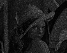
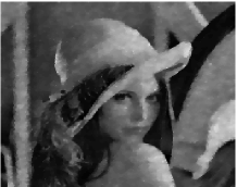
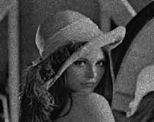
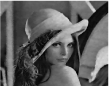
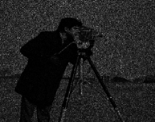
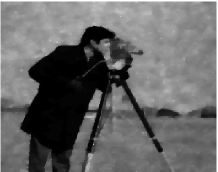
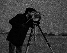
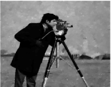
Fig. 1: Left column: observed noisy images. Right column: image estimates. First and second rows: Lena, $M=5$ and $M=33$. Third and fourth rows: Cameraman, $M=3$ and $M=13$.

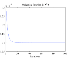
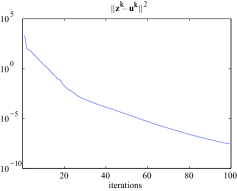
Fig. 2: Evolution of the objective function $L({\bf z}^{k})$ and of the constraint function $\|{\bf z}^{k}-{\bf u}^{k}\|_{2}^{2}$, along the iterations of the algorithm, for the experiment with the Cameraman image and $M=3$.

5 Concluding Remarks

We have proposed an approach to total variation denoising of images contaminated by multiplicative noise, by exploiting a split Bregman technique. The proposed algorithm is very simple and, in the experiments herein reported, exhibited state of the art performance and speed. We are currently working on extending our methods to problems involving linear observation operators (e.g., blur) and other related noise models, such as Poisson.

References

- [1] G. Aubert and J. Aujol, “A variational approach to remove multiplicative noise”, SIAM Jour. Appl. Math., vol. 68, no. 4, pp. 925–946, 2008.
- [2] J. Bioucas-Dias, T. Silva, and J. Leitão, “Adaptive restoration of speckled SAR images”, IEEE Intern. Geoscience and Remote Sensing Symposium, vol. I, pp. 19–23, 1998.
- [3] A. Chambolle, “An algorithm for total variation minimization and applications,” Jour. Math. Imaging and Vision, vol. 20, pp. 89-97, 2004.
- [4] T. Chan, S. Esedoglu, F. Park, and A. Yip, “Recent developments in total variation image restoration,” in Mathematical Models of Computer Vision, Springer, 2005.
- [5] T. Chan, G. Golub, and P. Mulet, “A nonlinear primal-dual method for total variation-based image restoration”, SIAM Jour. Sci. Comput., vol. 20, pp. 1964–1977, 1999.
- [6] P. Combettes and V. Wajs, “Signal recovery by proximal forward-backward splitting,” SIAM Jour. Multiscale Modeling & Simulation, vol. 4, pp. 1168–1200, 2005.
- [7] R. Corless, G. Gonnet, D. Hare, D. Jeffrey, and D. Knuth, “On the Lambert W function”, Adv. Computational Math. vol. 5, pp. 329–359, 1996.
- [8] M. Figueiredo, J. Bioucas-Dias, J. Oliveira, and R. Nowak, “On total-variation denoising: A new majorization-minimization algorithm and an experimental comparison with wavalet denoising,” IEEE Intern. Conf. Image Processing – ICIP’06, 2006.
- [9] V. Frost, K. Shanmugan, and J. Holtzman, “A model for radar images and its applications to adaptive digital filtering of multiplicative noise”, IEEE Trans. Pattern Analysis and Machine Intelligence, vol. 2, pp. 157–166, 1982.
- [10] T. Goldstein and S. Osher, “The split Bregman method for L1 regularized problems”, Tech. Rep. 08-29, Computational and Applied Math., Univ. of California, Los Angeles, 2008.
- [11] J. Goodman, “Some fundamental properties of speckle”, Jour. Opt. Soc. Amer., vol. 66, pp. 1145–1150, Nov. 1976.
- [12] Y. Huang, M. Ng, and Y. Wen, “A new total variation method for multiplicative noise removal”, SIAM Jour. Imaging Sciences, vol. 2, no. 1, pp. 20–40, 2009.
- [13] J. Nocedal and S. Wright, Numerical Optimization, Springer, 2006.
- [14] C. Oliver and S. Quegan, Understanding Synthetic Aperture Radar Images, Artech House, 1998.
- [15] S. Osher, L. Rudin, and E. Fatemi, “Nonlinear total variation based noise removal algorithms,” Physica D, vol. 60, pp. 259–268, 1992.
- [16] L. Rudin, P. Lions, and S. Osher, “Multiplicative denoising and deblurring: theory and algorithms”, in Geometric Level Set Methods in Imaging, Vision, and Graphics, S. Osher and N. Paragios (editors), pp. 103–120, 2003.
- [17] J. Shi and S. Osher, “A nonlinear inverse scale space method for a convex multiplicative noise model”, Tech. Rep. 07-10, Computational and Applied Math., Univ. of California, Los Angeles, 2007.
- [18] X. Tai and C. Wu, “Augmented Lagrangian method, dual methods and split Bregman iteration for ROF model”, Tech. Rep. 09-05, Computational and Applied Math., Univ. of California, Los Angeles, 2009.
- [19] Y. Wang, J. Yang, W. Yin, and Y. Zhang, “A new alternating minimization algorithm for total variation image reconstruction”, SIAM Jour. Imaging Sciences, vol. 1, no. 3, pp. 248–272, 2008.
- [20] W. Yin, S. Osher, D. Goldfarb, J. Darbon, “Bregman iterative algorithms for -minimization with applications to compressed sensing”, SIAM Jour. Imaging Sciences, vol. 1, no. 1, pp. 143–168, 2008.
- [21] M. Zhu, S. Wright, and T. Chan, “Duality-based algorithms for total variation image restoration”, Tech. Rep. 08-33, Computational and Applied Math., Univ. of California, Los Angeles, 2008.