Enhanced observability of quantum post-exponential decay using distant detectors

Abstract

We study the elusive transition from exponential to post-exponential (algebraic) decay of the probability density of a quantum particle emitted by an exponentially decaying source, in one dimension. The main finding is that the probability density at the transition time, and thus its observability, increases with the distance of the detector from the source, up to a critical distance beyond which exponential decay is no longer observed. Solvable models provide explicit expressions for the dependence of the transition on resonance and observational parameters, facilitating the choice of optimal conditions.

I Introduction

Exponential decay results when the decay rate depends linearly on the surviving population. It is observed in many quantum systems, in virtually all fields of physics (particle, nuclear, atomic, molecular, and condensed matter), but its microscopic derivation from the Schrödinger equation is not as straighforward as in classical physics, due to initial state reconstruction isr , and deviations are predicted at both short and long times FGR78 ; FP08 ; book . The Zeno effect, in particular, is associated with the short time deviation. The deviations at long times are less often discussed, and constitute the central topic of this paper.

On the experimental side, the post-exponential regime, which is typically algebraic, has been elusive. There have been many attempts to produce evidence of post-exponential decay, with little success Nik68 ; No88 ; Gr88 ; No95 ; Nghiep98 . It has been argued that repetitive measurements on the same system, or simply the interaction with the environment would lead to persistence of the exponential regime to times well beyond those expected in an isolated system FGR78 ; Greenland86 ; Law02b . Nevertheless a recent measurement of transitions from exponential to post-exponential decay of excited organic molecules in solution RHM06 appears to contradict this expectation, and has triggered renewed interest in the topic.

Aside from the non-trivial challenge of understanding and extending these experimental results, there are many reasons for studying post-exponential decay: Winter, for example, argued that hidden-variable theories could produce observable effects in samples that have decayed for many life-times Winterh ; more recently Krauss and Dent have pointed out that late-time decay may have important cosmological implications KD08 ; decay at long times is quite sensitive to delicate measurement and/or environmental effects, so it is a testing ground for theories of these processes; at a fundamental level, the form of long time deviations from exponential decay might distinguish between standard, Hermitian quantum mechanics DS84 , and modifications with a built-in microscopic arrow of time NB77 ; Nicolaides02 ; from a practical perspective, Norman pointed out that post-exponential decay could set a limit to the validity of radioactive dating methods No95 ; we have also argued that the deviation could be used to characterize certain cold atom traps MMS08 . Indeed, due to technological advances in lasers, semiconductors, nanoscience, and cold atoms, microscopic interactions are now relatively easy to manipulate: this makes decay parameters controllable, and post-exponential decay more accessible to experimental scrutiny and/or applications. For example, under appropriate conditions it could become the dominant regime and be used to speed-up decay, implementing an Anti-Zeno effect Lewenstein . In addition, recent experiments on periodic waveguide arrays provide a classical, electric field analog of a quantum system with exponential decay Lon06a ; VLL07 . These experiments may also reach the post-exponential region in a particularly simple way.

Most of the proposals to enhance post-exponential decay, making it more visible by advancing its onset time, are based on the idea of observing the survival probability for a resonance close to threshold (“small Q-value decay”) Jittoh ; GV06 ; RLE82 ; ZRL84 ; Lewenstein ; RHM06 , or more precisely, with energy release comparable to resonance width. This is a rare configuration in naturally decaying systems, such as radioactive isotopes RHM06 , or it leads to difficult measurements ZRL84 ; Greenland86 ; Kelkar , and realizing it in artificial structures, although possible in principle, is still a pending task Jittoh . The only realization so far may be the experiment on organic molecules in solution, mentioned above RHM06 , but this is a rather complex system and its analysis from first principles has not yet been performed, so the true mechanism behind the observed data remains to be confirmed. Another idea is to use the escape of interacting cold atoms from a trap, in the strongly interacting Tonks-Girardeau regime, to enhance the signal DDGMR06 . Again, the corresponding experiment has not yet been done. We also mention the proposal of Kelkar and coworkers Kelkar to deduce, rather than observe directly, the long-time decay characteristics from phase-shift data.

In the present paper we propose a quite different strategy with the important advantage of simple implementation. We show, using solvable decay models, that by increasing the distance of the observation point from the source, the transition from exponential to post-exponential decay occurs at higher probability densities, and thus becomes more easily observable. Figure 1 shows the probability density versus time, for three positions, and illustrates the density increase at the transition as the observation position $x$ is increased. (The details of the model will be explained in Sec. II.) The observability of the transition may additionally be enhanced by amplifying the signal with a macroscopic Bose-Einstein condensate wavefunction as explained in the final discussion. The combination of enhancing factors makes it possible to predict the observability of the transition for longer lifetimes than those implied by the above mentioned “small Q-value” condition.

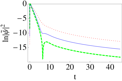
Figure 1: (Color online) Probability density versus $t$ for a fixed value of $k_{0}=1-0.5i$. Three detector positions $x$ have been considered: $x=1.5$ (red dotted line), $x=0.4$ (blue solid line), and $x=0.1$ (green dashed line). The dimensionless variables and the model are explained in Sec. II.

Finally, note that when the distance is too large the exponential decay regime disappears, and with it the transition, so that only non-exponential decay should be observed Newton .

In Section II a simple decay model is introduced and solved exactly. Section III provides approximate expressions useful to define the transition from exponential to post-exponential decay discussed in Section IV. The final section provides examples of possible physical realizations and compares the results with those of a discretized site model.

II Exponentially decaying source model and exact solution

There is a long and fruitful tradition of analytically solvable models for studying diverse aspects of single particle quantum dynamics. Closest to the model proposed here are several “source models” to examine quantum transients (propagation of signals, diffraction in time, forerunners) and tunneling dynamics of evanescent waves MB . Many works have been carried out within this approximation to study neutron interferometry FMGG90 ; BSCK92 , atom-wave diffraction BZ97 , tunneling dynamics Stevens ; Ranfa90 ; Ranfa91 ; Mor92 ; BT98 ; MB ; DMRGV , absorbing media DMR04 , different aperture functions FMGG90 ; BZ97 ; DM05 , and to model the dynamics of a guided atom laser DMM07 .

In these “source models”, unlike the usual initial value problem, the wave function is specified for all times at one point of coordinate space. (The connection between initial value problems and source boundary conditions has been discussed in BEM01 ). A simple, solvable 1D case corresponds to switching-on the source suddenly at $T=0$, with a well defined “carrier frequency” $\Omega_{0}>0$,

$$\Psi(0,T)=\Theta(T)e^{-i\Omega_{0}T},$$ (1)

zero external potential, $V=0$, and a vanishing wave everywhere (for all $X$) before the source is switched on, i.e. for $T<0$. The solution of the Schrödinger equation for $X>0$ is identical to that for the “Moshinsky shutter”, i.e. a wave created by the sudden opening of an opaque shutter which totally reflects an incident plane wave with reflection amplitude $r=1$ BZ97 prior to $T=0$. This solution shows the “diffraction in time” phenomenon of a fairly well-defined wavefront advancing with velocity $K_{0}\hbar/m$, where

$$K_{0}=\sqrt{2m\Omega_{0}/\hbar}$$ (2)

and $m$ is the mass of the particle. Negative values of $\Omega_{0}$ correspond to particle injection with energy below the potential threshold and may also be considered: interesting transients are produced in this way and, at long times, a stationary evanescent wave which penetrates into the classically forbidden region BT98 ; MB . Here we shall work out a case that has not yet been examined, namely, a complex carrier frequency $\Omega_{0}=\Omega_{0R}+i\Omega_{0I}$.

We assume a negative imaginary part, $\Omega_{0I}<0$, so that the density at the source point decreases exponentially,

$$|\Psi(0,T)|^{2}=e^{-2|\Omega_{0I}|T}.$$ (3)

The real part $\Omega_{0R}$ is chosen to be positive so as to generate travelling waves released from the source, and thus mimic the behaviour of resonance decay above threshold, in the outer region (outside the interaction region that holds the resonance).

This provides a simple (minimal) solvable model for an exponentially decaying system with a long lived resonance, while avoiding a detailed description of the interaction region where the decaying system is prepared. For many applications, and in particular during the exponential decay of the initial state, these details are unnecessary in the outer region, which in our case is represented by the positive half-line. We have also checked, see the final discussion, the broad validity of the results obtained using a different, complementary, norm-conserving, discretized lattice model. In it, the particle is prepared in the first site, which plays the role of the initial trap from which it escapes. This discretized model can be realized in periodic waveguide arrays, making use of an electric field analog of the quantum system Lon06a ; VLL07 .

II.1 The dimensionless Schrödinger equation

The dynamics of a particle in free space, $V=0$, is given by the Schrödinger equation

$$i\hbar\frac{\partial\Psi}{\partial T}=-\frac{\hbar^{2}}{2m}\frac{\partial^{2}\Psi}{\partial X^{2}}.$$ (4)

Let us first reduce the number of variables by introducing dimensionless quantities for position, time and wave function, in terms of some characteristic length $L$:

$$x = X/L,$$ (5)

$$t = \frac{T\hbar}{2mL^{2}},$$ (6)

$$\psi(x,t) = \sqrt{L}\,\,\Psi(X,T).$$ (7)

$L$ may be chosen for convenience and we take it as $K_{0R}^{-1}$, where $K_{0}=(2m\Omega_{0}/\hbar)^{1/2}=K_{0R}+iK_{0I}$ is the dimensioned complex wave number and $K_{0R}$ its real part. The branch cut is drawn just below the negative real axis so that for $\Omega_{0I}<0$ the imaginary part of $K_{0I}$ is negative, $K_{0I}:={\rm{Im}}(K_{0})<0$. Defining dimensionless wavenumber and carrier frequency as $k_{0}=K_{0}L$, and $\omega_{0}=\Omega_{0}2mL^{2}/\hbar=k_{0}^{2}$, this election fixes the real part of the dimensionless wave number to be unity, $k_{0R}=1$, and the dimensionless dispersion equation becomes

$$\omega_{0}=k_{0}^{2}=(1+ik_{0I})^{2},$$ (8)

where $-1<k_{0I}<0$. In terms of these new variables, the Schrödinger equation (4), is now

$$i\frac{\partial\psi(x,t)}{\partial t}=-\frac{\partial^{2}\psi(x,t)}{\partial x^{2}},$$ (9)

and the dimensionless continuity equation is

$$\frac{\partial\rho(x,t)}{\partial t}+\frac{\partial J(x,t)}{\partial x}=0,$$ (10)

where

$$\rho(x,t) = |\psi(x,t)|^{2},$$ (11)

$$J(x,t) = 2\,{\rm Im}\left[\psi^{*}(x,t)\frac{\partial\psi(x,t)}{\partial x}\right],$$ (12)

are the dimensionless probability and current densities.

II.2 Explicit solution

We are interested in waves that decay exponentially in time so the Schrödinger equation must satisfy boundary conditions at the origin

$$\psi(0,t)=e^{-i\omega_{0}t}\theta(t),\;\;\;\;\omega_{0R}>0,\,\omega_{0I}<0,$$ (13)

and at infinity, where the wave remains bounded as $x\to\infty$. which guarantees that the wave function does not diverge at $x=\infty$.

To find the solution for $x>0$ we make the ansatz

$$\psi(x,t)=\int_{-\infty}^{\infty}\!\!d\omega\,A(\omega)e^{i\sqrt{\omega}x}e^{-i\omega t},$$ (14)

and determine the function $A(\omega)$ from the boundary condition (13),

$$\psi(0,t)=e^{-i\omega_{0}t}\theta(t)=\int_{-\infty}^{\infty}\!\!d\omega\,A(\omega)e^{-i\omega t}.$$ (15)

Inverting the Fourier transform we obtain

$$A(\omega)=\frac{i}{2\pi(\omega-\omega_{0})},$$ (16)

The resulting integral for $\psi(x,t)$ is done most easily in the complex $k$ plane,

$$k=\sqrt{\omega}.$$ (17)

We may rewrite Eq. (14) for the wave function as

$$\psi(x,t)=\frac{-1}{2\pi i}\int_{\downarrow_{\rightarrow}}\!\!dk\,e^{-i(k^{2}t-kx)}\left(\frac{1}{k+k_{0}}+\frac{1}{k-k_{0}}\right),$$ (18)

where the branch cut for $k=\sqrt{\omega}$ (or $k_{0}=\sqrt{\omega_{0}}$) is chosen as before, slightly below the negative real axis. The integration path runs first from $i\infty$ to $\infty$ in the complex $k$-plane, but using Cauchy’s theorem it can be deformed into the diagonal path $\Gamma_{+}$ in the second and fourth quadrants passing above the pole at $-k_{0}$ in the second quadrant,

$$\psi(x,t)=\frac{-1}{2\pi i}\int_{\Gamma_{+}}\!\!dk\,e^{-i(k^{2}t-kx)}\left(\frac{1}{k+k_{0}}+\frac{1}{k-k_{0}}\right),$$ (19)

which may be split into two integrals of the form

$$\mathfrak{I}=\int_{\Gamma_{+}}\!\!dk\,\frac{e^{-i(ak^{2}+bk)}}{k-k_{p}},\;\;\;a>0,$$ (20)

The saddle point of the exponent is at $(k_{R}=-b/2a,k_{I}=0)$ and the steepest descent path is the straight line $k_{R}=-(k_{I}+b/2a)$. These integrals have been studied in MB by contour deformation into the steepest descent path. Independently of the pole position at $u_{p}=u(k_{p})$, the result is

$$\mathfrak{I}=-i\pi e^{ib^{2}/4a}w(-u_{p}),$$ (21)

where $w(z):=e^{-z^{2}}{\rm{erfc}}(-iz)$ is the Faddeyeva- (or “$w$”)-function FT61 ; AS65 , and $u_{p}=u(k_{p})$, where

$$u(k)=\sqrt{\frac{a}{2}}(1+i)(k+b/2a),$$ (22)

which becomes real along the (straight) steepest descent line, and vanishes at the saddle point.

Now we return to Eq. (19) where $a=t$ and $b=-x$, so the saddle point is at $k_{s}=x/(2t)$: this corresponds to the velocity of a classical particle that arrives at $x$ at time $t$ having departed from the origin at $t=0$. The steepest descent path is the straight line $k_{I}=-[k_{R}-x/(2t)]$. Applying Eq. (21), the wave function can finally be written as

$$\psi(x,t)=\frac{1}{2}e^{ik_{s}^{2}t}\left[w(-u_{0}^{(+)})+w(-u_{0}^{(-)})\right],$$ (23)

where

$$u_{0}^{(+)} = u(k_{0})=(1+i)\sqrt{\frac{t}{2}}k_{0}(1-\tau/t),$$ (24)

$$u_{0}^{(-)} = u(-k_{0})=-(1+i)\sqrt{\frac{t}{2}}k_{0}(1+\tau/t),$$ (25)

and the modulus of the complex time

$$\tau=\frac{x}{2k_{0}}$$ (26)

generalizes the Büttiker-Landauer traversal time, at least formally, in the present context MB .

II.3 Wave function normalization

For a fair comparison between different $k_{0}$ values, the total number of emitted particles must be kept fixed for all $k_{0}$, so the wave fuction must be normalized. The normalization constant can be obtained from the continuity equation (10) by integration,

$$N_{+}(t=\infty)=\int_{0}^{\infty}\!\!dt\,J(0,t),$$ (27)

where

$$N_{+}(t)=\int_{0}^{\infty}\!\!dx\,\rho(x,t)$$ (28)

is the norm, counting particles emitted to $x\geq 0$.

As we assume that one particle is emitted as $t\rightarrow\infty$, the normalized wave function, denoted by a tilde, is

$$\tilde{\psi}(x,t)=\frac{1}{\sqrt{\int_{0}^{\infty}\!\!dt\,J(0,t)}}\psi(x,t).$$ (29)

III Asymptotic behaviour

The exact solution is useful but not necessarily physically illuminating, whereas approximations often provide a more transparent physical interpretation. To this end we separate each $w$-function term into the contribution of the saddle point $k=k_{s}$, and a pole contribution. The dominant contribution of the saddle is obtained from Eq. (19) by setting $k=k_{s}$ in the denominators and integrating along the steepest descent path,

$$\psi_{s}(x,t) = \frac{1}{2i\sqrt{\pi}}\left(\frac{1}{u^{(+)}_{0}}+\frac{1}{u^{(-)}_{0}}\right)$$ (30)

$$= \sqrt{\frac{2t}{\pi}}\frac{\tau e^{ik_{s}^{2}t}}{(i-1)k_{0}(t^{2}-\tau^{2})}.$$

After the steepest descent path crosses the pole $k_{0}$ when ${\rm Im}{u_{0}^{(+)}}=0$, its residue $\psi_{0}(x,t)$ must be added to the saddle wave function $\psi_{s}$, see Fig. 2,

$$\psi_{0}=e^{ik_{s}^{2}t}e^{-u_{0}^{(+)2}}=e^{-i\omega_{0}t}e^{ik_{0}x}.$$ (31)

(Note that the pole at $-k_{0}$, in the fourth octant, is never crossed.) A travelling wave component moving rightwards is generated. For fixed $t$ the exponential decay is imprinted in $e^{ik_{0}x}$: because of the negative imaginary part of $k_{0}$ the wave increases rightwards in coordinate space until the $x$ value satisfying ${\rm Im}{u_{0}^{(+)}}=0$. Of course the full wave does not show this sharp edge but a smoothed one.

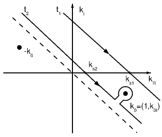
Figure 2: $k$-plane with contour deformations along the steepest descent paths (SDP) (the straight lines) at times $t_{2}>t_{1}$, and saddle points $k_{s1}$, $k_{s2}$. At $t_{1}$, the $k_{0}$ pole has not yet been crossed, while at $t_{2}$ the pole has been crossed and encircled by the keyhole contour. The dashed line is the SDP for $t\sim\infty$, showing that the pole at $-k_{0}$ is never crossed.

It follows that the total wave function can be approximated as

$$\psi(x,t)=\psi_{s}(x,t)+\psi_{0}(x,t)\,\Theta[\mbox{Im}(u_{0}^{(+)})].$$ (32)

To see the conditions for validity of this expression, note that the first and the exponential terms in the asymptotic series expansion for $w(z)$ at large $|z|$,

$$w(z) \sim \frac{i}{\sqrt{\pi}z}\left[1+\sum_{m=1}^{\infty}\frac{1\times 3\times\ldots\times(2m-1)}{(2z^{2})^{m}}\right]$$ (33)

$$+ 2e^{-z^{2}}\,\,\Theta[-{\rm Im}(z)],$$

do reproduce Eq. (32). In our case, large $z$ means large $u_{0}^{(\pm)}$. Their moduli can be written as

$$|u_{0}^{(\pm)}|=\sqrt{x|k_{0}|}\sqrt{\frac{t}{2|\tau|}\pm\frac{1}{|k_{0}|}+\frac{|\tau|}{2t}},$$ (34)

which take large values in certain conditions, in particular at times short and long compared to $|\tau|$.

IV Transition from exponential to post-exponential decay

The criterion which sets the time scale of the transition, is that the moduli of pole and saddle contributions to the total density are equal. We thus identify the transition as the space-time point where their ratio $R(x,t)$ is one,

$$|\psi_{0}|^{2} = e^{2{\rm{Im}}(\omega_{0}t-k_{0}x)},$$ (35)

$$|\psi_{s}|^{2} = \frac{t|\tau|^{2}}{\pi|k_{0}|^{2}[t^{4}+|\tau|^{4}-2t^{2}{\rm Re}(\tau^{2})]},$$ (36)

$$R(x,t) = \frac{|\psi_{0}|}{|\psi_{s}|}=\frac{2\sqrt{\pi}|k_{0}|^{2}\,t^{3/2}}{x}e^{{\rm Im}(\omega_{0}t-k_{0}x)}$$ (37)

$$\times \sqrt{1+\frac{|\tau|^{4}}{t^{4}}-2{\rm Re}\left(\frac{\tau^{2}}{t^{2}}\right)}.$$

In addition, the condition ${\rm Im}(u_{0}^{(+)})>0$ (the pole has been crossed by the steepest descent path) must be verified.

Solving $R(x,t)=1$ with the assumption $t>>|\tau|$, we obtain an expression for the transition time $t_{p}$ for fixed $x$,

$$t_{p}^{3/2}=\frac{xe^{-{\rm Im}(\omega_{0}t_{p}-k_{0}x)}}{2\sqrt{\pi}|k_{0}|^{2}}.$$ (38)

The transition is generally not sharply defined in the exact density, and is characterized by interference fringes due to the superposition of saddle and resonance contributions.

In the following we shall investigate the behaviour of the probability density at the transition point $t_{p}$, when the parameters $x$ and/or the imaginary part $k_{0I}$ of $k_{0}$ are varied. First we fix $k_{0}$ and observe the density as a function of $t$ for different $x$-values. A global 3D plot is shown in Fig. 3, in which we chose $k_{0I}$ to highlight the dominance of exponential decay at small $x$ and post-exponential at large $x$. The pole (straight lines) and saddle densities for three values of $x$ are shown in Fig. 4, in which $x$ increases from the dotted to solid to dashed lines.

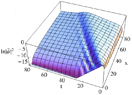
Figure 3: Overview of the Log probability density in the $t$, $x$ plane, for fixed $k_{0}=1-0.15i$.

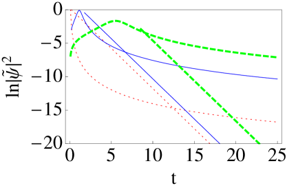
Figure 4: (Color online) Probability density versus time, for three $x$ values, at fixed $k_{0}=1-0.3i$. The crossing point between the pole (straight line) and saddle terms defines the transition time $t_{p}$. Dotted (red) line: $x=0.1$, crossing at $t_{p}=12$; solid (blue) line: $x=2.5$, crossing at $t_{p}=7$: and dashed (green) line: $x=12$, crossing at $t_{p}=9$.

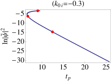
Figure 5: Probability density versus $t_{p}(x)$ at the transition point for fixed $k_{0}=1-0.3i$. The drawing covers $x$ running from $0.0001$ to $13$. The dots correspond to the $x$ values considered in Fig. 4.

Several interesting conclusions can be inferred from these figures and the corresponding equations (36,37,38). An important one is that the probability density at the transition point increases, as the observation point is moved away from the source, improving the possibility of observing the transition. A basic reason for this is the asymptotic growth of $|\psi_{s}|^{2}\sim x^{2}$, whereas the pole term density (straight line in Fig. 4) is basically shifted by $\delta x/2k_{0R}$ for a shift $\delta x$ in the observation coordinate: in other words, the exponential behaviour is delayed by increasing $x$.

Note also the behaviour of the transition time $t_{p}$ as $x$ increases. Initially $t_{p}$ occurs earlier as $x$ increases, but there is an $x$ value, $x=1/|k_{0I}|$, beyond which the tendency changes, and $t_{p}$ then increases with $x$ until the transition is no longer observable, as the onset of the exponential decay contribution is below the saddle contribution. Figure 5 shows the density at the transition versus $t_{p}$. The curve depends parametrically on $x$, which increases from the bottom right corner upwards. The last point marks the largest value of $x$ for which the transition may be defined by the $R=1$ criterion, and such that ${\rm Im}(u_{0}^{(+)})>0$. This value of $x$ corresponds very nearly to the case depicted by dashed lines in Fig. 4. This maximum $x$ increases with the resonance lifetime $\tau_{0}=1/|4k_{0I}|$, and it is plotted versus $|k_{0I}|$ in Fig. 6. The (normalized, see Sec. II.3) density at that critical point is shown in Fig. 7. We can infer from this figure that there is a maximum of the transition point density slightly to the right of $k_{0I}\sim-0.5$. This is consistent with the condition described by Jittoh Jittoh for purely non-exponential decay,

$${\Gamma}/{\epsilon}={1}/[{k_{0R}^{2}\tau_{0}}]=4|k_{0I}|\geq 2,$$ (39)

where $\Gamma$ and $\epsilon$ are the (dimensionless) decay rate and real energy of the resonance, and we have used the fact that the real part $k_{0R}=1$ in our units.

We are now better prepared to come back to Fig. 3 and appreciate several of its features: note the exponential decay at the $x=0$ edge, the linear delay of the approximate wave front when $x$ is increased, the increase of the algebraic long-time tail with $x$, and the characteristic transition fringes at intermediate $x$ values, which disappear for larger $x$ values, characterized by purely non-exponential behavior.

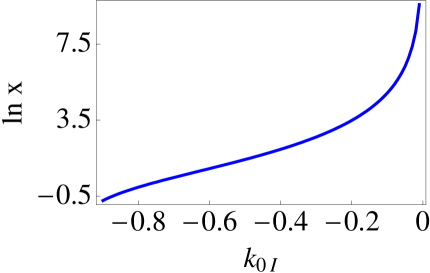
Figure 6: Largest $x$ value where an exponential to post-exponential transition is found, satisfying the conditions $R=1$ and ${\rm{Im}}u_{0}^{(+)}>0$, versus $k_{0I}$ (normalized waves).

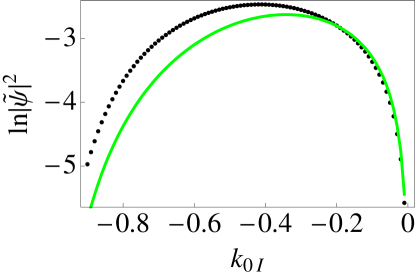
Figure 7: (Color online) Density of normalized waves, at the largest $x$ value where the transition is defined, as function of $k_{0I}$. Solid (green) line: density of the approximate solution; Dotted (black) line: value from the exact wavefunction.

V Discussion

The transition from exponential to non-exponential decay for an isolated decaying system has never been observed despite the well-established theoretical prediction that it must eventually occur. Apart from the difficulty of avoiding interactions that may extend the exponential region, a fundamental reason is the small value of the survival probability at the predicted transition. We have shown that observing the density of decay products at an optimal distance from the source, significantly improves the observability of this elusive transition. Almost 50 years ago R. G. Newton Newton gave a classical-trajectory argument pointing out that the transition would be affected by the observation distance. His predicted behaviour and dependence on parameters do not, however, coincide with the present quantum results. We have put forward a simple decay model that provides analytical expressions, facilitates predictions, and allows analysis of a proposed experiment through its dependence on resonance and observation parameters (release energy and lifetime, distance and time of density measurement). Experiments may be undertaken using quantum systems such as a leaking quantum dot, or escape of ultracold atoms from a trap. In both cases, trap and escape parameters are controllable, and it is possible to set a time zero for preparation of the decaying system. An effective 1D waveguide (a quantum wire for electrons, or a detuned laser for atoms) may channel the escaping particle away from the trap. Localized, or spatially resolved particle detection can be performed, e.g., with fluorescence or absorption techniques. Experimentally accessible low temperatures and conditions determine decoherence lengths and times, large enough to observe the effects described. Atom-atom interactions may be minimized by using Feshbach resonances. As an example, let us consider an ⁸⁷Rb quasi-one dimensional Bose-Einstein condensate sample of $10^{6}$ atoms, released to a quasi-1D waveguide from a controllable trap that will determine the resonance energy and lifetime prepa . Then a commercial CCD camera with $\sim 3$ $\mu$m spatial resolution and shot noise limited detection with at least $\sim 10$ atoms/pixel may be used to measure the atomic density at the waveguide by resonant absorption imaging kruger . According to our model a sample of $10^{6}$ atoms with lifetime $\sim 400$ $\mu$s, and release velocity $\sim 1$ cm/s would provide a $9200$ atoms/pixel transition density at $t_{p}\sim 10$ ms and at a distance of $\sim 100$ $\mu$m. These numbers make the observation of the transition very plausible. Note that even $10^{3}$ initial atoms would be close to the shot-noise observation limit at that space-time point. An analysis of the effect of atom-atom interactions in the condensate is left for a separate study but, it is expected that such interactions will not be significant in the transition densities.

A different physical realization may be possible through an array of long parallel waveguides Jo65 ; CLS03 . The variation with $z$, (the longitudinal distance along the guide) of the electric field in the $n$’th guide, plays the role of the variation with time of the site amplitudes of a quantum tight-binding model Lon06a ; VLL07 . Recent experiments with scanning tunnelling microscopy have allowed Longhi and collaborators VLL07 to measure the evanescent fields along the waveguides, and demonstrate the classical-quantal analogy for a periodic parallel array. In addition Bia08 the classical analogue of the quantum Zeno effect has been verified.

If the coupling between adjacent sites, except for the first two, is described by a universal hopping constant, and the site energies are taken all to be equal, the Hamiltonian is, in dimensionless units,

$$H = -\Delta\bigg{[}|1\rangle\langle 2|+|2\rangle\langle 1|\bigg{]}$$ (40)

$$- \sum_{n=2}^{\infty}\,\bigg{[}|n\rangle\langle n+1|+|n+1\rangle\langle n|\bigg{]},$$

where we take $0<\Delta<1$ to provide isolation of site $1$ from the rest of the array.

When only site $1$ is occupied at time zero, the analytic solution for the amplitude at site $n$ shows a transition from exponential to power-law decay, at the time defined by equating the exponential contribution to the asymptotic power-law decay expression, dropping a sinusoidal oscillation peculiar to this model.

$$t^{3/2}=\frac{[n+\alpha^{2}(n-2)]}{\sqrt{\pi}(1+\alpha^{2})^{3}}{2\alpha^{n+1}}e^{\gamma t/2}.$$ (41)

where $\alpha^{2}=1-\Delta^{2}$, and $\gamma=2\Delta^{2}/\alpha$. For small $\Delta$, $|\alpha|\sim 1$, making $\gamma<<1$, and giving a long lifetime for exponential decay. But so long as $|\alpha|<1$, $|\alpha|^{n+1}<<1$, for large enough $n$, allowing a solution to be found. (The oscillations in the power-law decay cause some imprecision in the transition time, similar to that discussed in relation to Fig. 3 for the model of this paper.) Eq. (41) is very similar to Eq. (38), and predicts the same phenomena. This provides support for the general validity of our main conclusion, namely, that the optimal transition density increases with increasing distance of the detector from the trap.

References

- (1) J. G. Muga, F. Delgado, A. del Campo, and G. García-Calderón, Phys. Rev. A 73, 052112 (2006), and references therein.
- (2) L. Fonda, G.C. Ghirardi, and A. Rimini, Rep. Prog. Phys. 41, 587 (1978).
- (3) P. Facchi and S. Pascazio, J. Phys. A: Math. Gen 41, 493001 (2008).
- (4) J. Martorell, J. G. Muga, and D. W. L. Sprung, in Time in Quantum Mechanics, Vol. 2, Springer, Berlin, 2009.
- (5) N. N. Nikolaev, Sov. Phys. Usp. 11, 522 (1968).
- (6) E. B. Norman, S. B. Gazes, S. G. Crane, and D. A. Bennett, Phys. Rev. Lett. 60, 2246 (1988).
- (7) P. T. Greenland, Nature 335, 298 (1988).
- (8) T. D. Nghiep, V. T. Hahn, N. N. Son, Nucl. Phys. B (Proc. Suppl.) 66, 533 (1998).
- (9) E. B. Norman, B. Sur, K. T. Lesko, R. M. Larimer, D. J. DePaolo, and T. L. Owens, Phys. Lett. B 357, 521 (1995).
- (10) P. T. Greenland, Phys. Lett. A 117, 181 (1986).
- (11) R. E. Parrott and J. Lawrence, Europhys. Lett. 57, 632 (2002).
- (12) C. Rothe, S. I. Hintschich, and A. P. Monkman, Phys. Rev. Lett. 96, 163601 (2006).
- (13) R. G. Winter, Phys. Rev. 126, 1152 (1962).
- (14) L. M. Krauss and J. Dent, Phys. Rev. Lett. 100, 171301 (2008).
- (15) S. D. Druger and M. A. Samuel, Phys. Rev. A 30, 640 (1984).
- (16) C. A. Nicolaides and D. R. Beck, Phys. Rev. Lett. 38, 683, 1037 (1977)
- (17) C. A. Nicolaides, Phys. Rev. A 66, 022118 (2002).
- (18) J. Martorell, J. G. Muga, and D. W. L. Sprung, Phys. Rev. A 77, 042719 (2008).
- (19) M. Lewenstein and K. Rzazewski, Phys. Rev. A 61, 022105 (2000).
- (20) S. Longhi, Phys. Rev. Lett. 97, 110402 (2006).
- (21) G. Della Valle, S. Longhi, P. Laporta, P. Biagioni, L. Dou, and M. Finazzi, Appl. Phys. Lett. 90, 261118 (2007).
- (22) T. Jittoh, S. Matsumoto, J. Sato, Y. Sato, K. Takeda, Phys. Rev. A 71, 012109 (2005).
- (23) G. García-Calderón, J. Villavicencio, Phys. Rev. A 73, 062115 (2006).
- (24) K. Rzazewski, M. Lewenstein, J. H. Eberly, J. Phys. B: At. Mol. Phys. 15, L661 (1982).
- (25) J. Zakrzewski, K. Rzazewski, M. Lewenstein, J. Phys. B: At. Mol. Phys. 17, 729 (1984).
- (26) N. G. Kelkar, M. Nowakowski, and K. P. Khemchandani, Phys. Rev. C 70, 024601 (2004).
- (27) A. del Campo, F. Delgado, G. García-Calderón, J. G. Muga and M. G. Raizen, Phys. Rev. A 74, 013605 (2006).
- (28) R. G. Newton, Annals of Physics (NY) 14, 333 (1961).
- (29) J. G. Muga and M. Büttiker, Phys. Rev. A 62, 023808 (2000).
- (30) J. Felber, G. Müller, R. Gähler, and R. Golub, Physica B 162, 191 (1990).
- (31) H. R. Brown, J. Summhammer, R. E. Callaghan and P. Kaloyerou, Phys. Lett. A, 163, 21 (1992).
- (32) C. Brukner and A. Zeilinger, Phys. Rev. A 56, 3804 (1997).
- (33) K. W. H. Stevens, Eur. J. Phys. 1, 98 (1980); J. Phys. C 16, 3649 (1983).
- (34) A. Ranfangi, D. Mugnai, P. Fabeni, and P. Pazzi, Phys. Scr. 42, 508 (1990).
- (35) A. Ranfangi, D. Mugnai, and A. Agresti, Phys. Lett. A 158, 161 (1991).
- (36) P. Moretti, Phys. Scripta 45, 18 (1992).
- (37) M. Büttiker, H. Thomas, Superlatt. Microstruct. 23, 781 (1998).
- (38) F. Delgado, J. G. Muga, A. Ruschhaupt, G. García-Calderón, J. Villavicencio, Phys. Rev. A 68 (2003) 032101.
- (39) F. Delgado, J. G. Muga, A. Ruschhaupt, Phys. Rev. A 69, 022106 (2004).
- (40) A. del Campo and J. G. Muga, J. Phys. A, 38, 9802 (2005).
- (41) A. del Campo, J. G. Muga, and M. Moshinsky, J. Phys. B 40, 975 (2007).
- (42) A. D. Baute, I. L. Egusquiza, J. G. Muga, J. Phys. A 34, 4289 (2001).
- (43) V. N. Faddeyeva, N. M. Terentev, Mathematical Tables: Tables of the values of the function for complex argument, Pergamon, New York, 1961.
- (44) A. Abramowitz, I. A. Stegun, Handbook of Mathematical Functions, Dover, New York, 1965.
- (45) F. Delgado, J. G. Muga, and A. Ruschhaupt, Phys. Rev. A 74, 063618 (2006).
- (46) P. Krüger, S. Wildermuth, S. Hofferberth, L. M. Andersson, S. Groth, I. Bar-Joseph, J. Schmiedmayer, J. Phys. Conference Series 19 (2005) 56-65.
- (47) A. L. Jones, J. Opt. Soc. Am. 55, 261-271 (1965).
- (48) D. N. Christodoulides, F. Lederer and Y. Silverberg, Nature 424, 817-23 (2003).
- (49) P. Biagoni, G. Della Valle, M. Ornigotti, M. Finazzi, L. Duo, P. Laporta and S. Longhi, Optics Express 16, 3762-7 (2008).