A comprehensive population synthesis study of post-common envelope binaries

Abstract

We apply population synthesis techniques to calculate the present day population of post-common envelope binaries (PCEBs) for a range of theoretical models describing the common envelope (CE) phase. Adopting the canonical energy budget approach we consider models where the ejection efficiency, $\alpha_{\mathrm{CE}}$ is either a constant, or a function of the secondary mass. We obtain the envelope binding energy from detailed stellar models of the progenitor primary, with and without the thermal and ionization energy, but we also test a commonly used analytical scaling. We also employ the alternative angular momentum budget approach, known as the $\gamma$-algorithm. We find that a constant, global value of $\alpha_{\mathrm{CE}}\ga 0.1$ can adequately account for the observed population of PCEBs with late spectral-type secondaries. However, this prescription fails to reproduce IK Pegasi, which has a secondary with spectral type A8. We can account for IK Pegasi if we include thermal and ionization energy of the giant’s envelope, or if we use the $\gamma$-algorithm. However, the $\gamma$-algorithm predicts local space densities that are 1 to 2 orders of magnitude greater than estimates from observations. In contrast, the canonical energy budget prescription with an initial mass ratio distribution that favours unequal initial mass ratios ($n(q_{\mathrm{i}})\propto{q_{\mathrm{i}}^{-0.99}}$) gives a local space density which is in good agreement with observations, and best reproduces the observed distribution of PCEBs. Finally, all models fail to reproduce the sharp decline for orbital periods, $P_{\mathrm{orb}}\ga 1$ d in the orbital period distribution of observed PCEBs, even if we take into account selection effects against systems with long orbital periods and early spectral-type secondaries.

1 Introduction

The common envelope (CE) phase was proposed by Paczyński (1976) to explain the small orbital separation of compact binaries such as cataclysmic variables (CVs) and double white dwarf binaries, because a much larger orbital separation of between approximately 10 and 1000 R_⊙ was required in order to accommodate the giant progenitor of the white dwarf. (For reviews see Iben & Livio 1993, Taam & Sandquist 2000).

In the pre-CE phase of evolution the initially more massive stellar component (which we henceforth denote as the primary) evolves off the main sequence first. Depending on the orbital separation of the binary, the primary will fill its Roche lobe on either the giant or asymptotic giant branch and initiate mass transfer. If the giant primary possesses a deep convective envelope (i.e. the convective envelope has a mass of more than approximately 50 per cent of the giant’s mass; Hjellming & Webbink 1987) the giant will expand in response to rapid mass loss. As a result, the giant’s radius expands relative to its Roche lobe radius increasing the mass transfer rate. As a consequence of this run-away situation, mass transfer commences on a dynamical timescale. The companion main sequence star (henceforth the secondary) cannot incorporate this material into its structure quickly enough and therefore expands to fill its own Roche lobe. The envelope eventually engulfs both the core of the primary and the main sequence secondary.

The friction the stellar components experience due to their motion within the CE extracts energy and orbital angular momentum from the orbit causing the orbital separation to decrease. If enough of the orbital energy is imparted on to the CE before the stellar components merge, then the CE may be ejected from the system leaving the core of the primary (now the white dwarf) and the secondary star at a greatly reduced separation.

Despite extensive three dimensional hydrodynamical simulations (e.g. Sandquist, Taam & Burkert 2000), the physics of the CE phase remains poorly understood, including the efficiency with which the CE is ejected from the system. Due to the difficulty in modelling the CE phase, binary population synthesis calculations commonly resort to describing the CE phase in terms of a simple energy budget argument. A fraction $\alpha_{\mathrm{CE}}$ of the orbital energy released as the binary tightens, $\Delta{E_{\mathrm{orb}}}$, is available to unbind the giant’s envelope from the core. Hence if the binding energy is $E_{\mathrm{bind}}$ we have

$$E_{\mathrm{bind}}=\alpha_{\mathrm{CE}}\Delta{E}_{\mathrm{orb}}$$ (1)

(e.g. de Kool 1992; de Kool & Ritter 1993; Willems & Kolb 2004). The efficiency $\alpha_{\mathrm{CE}}$ is a free parameter with values $0<\alpha_{\mathrm{CE}}\leq{1}$, albeit values larger than unity are discussed, depending on what terms are included in the quantity $E_{\mathrm{bind}}$.

Nelemans et al. (2000) used this approach to reconstruct the common envelope phase for the observed sample of double white dwarf binaries. They found that $\alpha_{\mathrm{CE}}<0$ for the first phase of mass transfer, which is unphysical. This led them to test an alternative description of the CE phase, based on the change in the orbital angular momentum of the binary, $\Delta{J}$, during the CE phase. Their ‘$\gamma$-algorithm’ follows the prescription given by Paczyński & Ziółkowski (1967),

$$\Delta{J}=\gamma\frac{JM_{\mathrm{env}}}{M_{\mathrm{b}}},$$ (2)

where $M_{\mathrm{env}}$ is the mass of the giant’s envelope, $M_{\mathrm{b}}$ is the total mass of the binary just before the onset of the CE phase and $J$ is the total angular momentum of the binary at this point. The free parameter $\gamma$ describes the specific angular momentum of the ejected material (in this case the CE) in units of the specific angular momentum of the binary system. Indeed, Nelemans & Tout (2005) found further support for the $\gamma$-algorithm in a few observed pre-CVs and sub-dwarf B plus main sequence star binaries.

Beer et al. (2007) suggested that some systems may avoid the in-spiral in a CE phase altogether as a result of wind ejection of the envelope material from the system, which arises due to super-Eddington accretion on to the companion star. Employing analytical approximations for the evolution of such systems, Beer et al. (2007) found that both the canonical energy budget approach and the $\gamma$-algorithm can describe the outcomes of the proposed mechanism.

A few observed double white dwarf binaries could also be explained by $\alpha_{\mathrm{CE}}>1$, for example, PG 1115+166 (Maxted et al., 2002). This has led to the suggestion that an energy source other than the release of orbital energy is being used to eject the CE from the system, such as thermal energy and recombination energy of ionized material within the giant’s envelope (Han et al. 1994, Han et al. 1995, Dewi & Tauris 2000, Webbink 2007).

Alternatively, Politano & Weiler (2007) suggested that rather than $\alpha_{\mathrm{CE}}$ being a constant, global value for all binary systems, it is a function of one of the binary orbital parameters. In this spirit, Politano & Weiler (2007) calculated the present day population of post-common envelope binaries (PCEBs) and CVs if $\alpha_{\mathrm{CE}}$ is a function of the secondary mass. The investigation was motivated by the fact that very few, if any, CVs with brown dwarf secondaries at orbital periods below 77 mins have been detected. This appears to be in conflict with Politano (2004) who estimated from his models that such systems should make up approximately 15 per cent of the current CV population. Politano (2004) suggested that this discrepancy may be a result of the decreasing energy dissipation rate of orbital energy within the CE for decreasing secondary mass, and that below some cut-off mass, a CE merger would be unavoidable.

Previous population synthesis studies into the CE phase of white dwarf-main sequence binaries(e.g. de Kool & Ritter 1993; Willems & Kolb 2004) just considered the value of the envelope’s binding energy, $E_{\mathrm{bind}}$, due to the gravitational binding energy of the primary’s envelope,

$$E_{\mathrm{bind}}=-\int^{M_{1}}_{M_{\mathrm{c}}}\frac{GM(r)}{r}\,\mathrm{d}m,$$ (3)

where $M(r)$ is the mass contained within the radius $r$ of the primary, $M_{\mathrm{c}}$ is the mass of the giant’s core, and $G$ is the universal gravitational constant. In population synthesis studies the binding energy is commonly approximated as

$$E_{\mathrm{bind}}=-\frac{GM_{1}M_{\mathrm{env}}}{\lambda R_{1}},$$ (4)

where $R_{1}$ is the radius of the primary star, with a suitable choice for the dimensionless factor $\lambda$.

de Kool (1992) and Willems & Kolb (2004) for example, used a constant, global value of $\lambda=0.5$. As Dewi & Tauris (2000) pointed out, however, this may lead to an overestimation of the giant envelope’s binding energy for large radii, requiring more energy to eject it.

In the present study we apply population synthesis techniques to calculate the present day population of PCEBs by considering the aforementioned theoretical descriptions of the CE phase. We consider different constant, global values of $\alpha_{\mathrm{CE}}$ and $\lambda$, $\alpha_{\mathrm{CE}}$ as a function of secondary mass, and $\lambda$ calculated according to the internal structure of the giant star and the internal energy of its envelope. Also, we consider the description of the CE phase is terms of the angular momentum budget of the binary system.

We then compare our model PCEB populations to the observed sample of white dwarf-main sequence star (WD+MS) and sub-dwarf-main sequence star (sd+MS) binaries from RKCat (Ritter & Kolb, 2003), Edition 7.10 (2008), and newly detected PCEBs from the Sloan Digital Sky Survey (SDSS) (Rebassa-Mansergas et al. 2007; Rebassa-Mansergas et al. 2008). We also compare this observational sample to our theoretical population for a range of initial secondary mass distributions.

Our suite of population models represents a major advance over the work by Willems & Kolb (2004) who considered only the formation rate of PCEBs, and a simplified estimate of their present-day populations based on birth and death rates. Our models also cover a more comprehensive parameter space than those by Politano & Weiler (2007), and we assess the model distributions against the location of observed systems in all three system parameters (component masses and period) simultaneously.

The structure of the paper is as follows. In Section 2 we give our computational method and models describing the CE phase. In Section 3 we present our results, which are discussed in Section 4. We conclude our investigation in Section 5.

2 Computational Method

We employ the same method as used in Davis et al. (2008) to calculate the binary population, and so we present only a summary here. We first calculate the unweighted zero-age PCEB population (i.e. WD+MS systems that have just emerged from a CE phase) with BiSEPS (Willems & Kolb 2002; Willems & Kolb 2004). BiSEPS employs the single star evolution (SSE) formulae described in Hurley, Pols & Tout (2000) and a binary evolution scheme based on that described by Hurley, Tout & Pols (2002). We then use a second code introduced in Willems et al. (2005) to calculate the present day population of PCEBs.

This latter step makes use of evolutionary tracks, calculated by BiSEPS, for each PCEB configuration, from the moment the PCEB forms to the point at which the binary ceases to be a PCEB (for example, if the system becomes semi-detached). BiSEPS therefore produces a library of PCEB evolutionary tracks which contain, depending on the population model, between $30\,000$ and $100\,000$ PCEB sequences.

2.1 Initial Binary Population

BiSEPS evolves a large number of binary systems, initially consisting of two zero-age main sequence stellar components. The stars are assumed to have a population I chemical composition and the orbits are circular at all times. The initial primary and secondary masses are in the range 0.1 to 20 M_⊙, while the initial orbital periods range from 0.1 to 100 000 d. There is one representative binary configuration per grid cell within a three-dimensional grid consisting of 60 logarithmically spaced points in primary and secondary mass and 300 logarithmically spaced points in orbital period. Hence we evolve approximately $5.4\times{10}^{5}$ binaries for a maximum evolution time of 10 Gyr. For symmetry reasons only systems where $M_{1}>M_{2}$ are evolved.

The probability of a zero-age PCEB forming with a given white dwarf mass $M_{\mathrm{WD}}$, secondary mass $M_{2}$ and orbital period $P_{\mathrm{orb}}$ is determined by the probability of the binary’s initial parameters. We assume that the initial primary mass, $M_{1,\mathrm{i}}$ is distributed according to the initial mass function (IMF) given by Kroupa, Tout & Gilmore (1993). The distribution of initial secondary masses, $M_{2,\mathrm{i}}$, is obtained from the initial mass ratio distribution (IMRD), $n(q_{\mathrm{i}})$, where $q_{\mathrm{i}}=M_{2,\mathrm{i}}/M_{1,\mathrm{i}}$, and $n(q_{\mathrm{i}})$ has a power-law dependence on $q_{\mathrm{i}}$. Alternatively, we determine $M_{2,\mathrm{i}}$ from the same IMF as used for the initial primary mass. For brevity, we adopt the acronym ‘IMFM2’ for this latter case. Our standard model is a flat distribution, i.e. $n(q_{\mathrm{i}})=1$. Finally, we follow Iben & Tutukov (1984) and Hurley, Tout & Pols (2002) and adopt a logarithmically flat distribution in initial orbital separations.

We assume that all stars in the Galaxy are formed in binaries, and that the Galaxy has an age of 10 Gyr. The aforementioned distributions are then convolved with a constant star formation rate normalised such that one binary with $M_{1,\mathrm{i}}>0.8$ M_⊙ is formed each year, consistent with observations (Weidemann, 1990). This gives an overall star formation rate of $7.6$ yr^-1.

Table 1: Different models on the treatment of the CE phase.

Model	$\alpha_{\mathrm{CE}}$ or $\gamma$	$\lambda$
A	1.0	0.5
CE01	0.1	0.5
CE06	0.6	0.5
PL05	eqn. (6), $p=0.5$,	0.5
PL1	eqn. (6), $p=1$,	0.5
PL2	eqn. (6), $p=2$,	0.5
CT0375	eqn. (7), $M_{\mathrm{cut}}/\mathrm{M}_{\odot}=0.0375$	0.5
CT075	eqn. (7), $M_{\mathrm{cut}}/\mathrm{M}_{\odot}=0.075$	0.5
CT15	eqn. (7), $M_{\mathrm{cut}}/\mathrm{M}_{\odot}=0.15$	0.5
DTg	1.0	$\lambda_{\mathrm{g}}$
DTb	1.0	$\lambda_{\mathrm{b}}$
n15	1.5, eqn. (8)	-

2.2 The Common Envelope Phase

Here we specify details of the different model descriptions used for the CE phase. These are also summarised in Table 1. In the energy budget approach the CE phase is modelled by equating the change in the binding energy of the primary’s envelope to the change in the orbital energy of the binary system (see Section 1, eqn. 1). Thus, the final orbital separation of the binary after the CE phase, $A_{\mathrm{CE,f}}$, is given by

$$A_{\mathrm{CE,f}}=A_{\mathrm{CE,i}}\frac{M_{\mathrm{c}}}{M_{1}}\left[1+\left(\frac{2}{\lambda\alpha_{\mathrm{CE}}r_{\mathrm{L},1}}\right)\left(\frac{M_{\mathrm{env}}}{M_{2}}\right)\right]^{-1}.$$ (5)

Here $A_{\mathrm{CE,i}}$ is the initial orbital separation at the onset of the CE phase, $M_{1}$ and $M_{2}$ are the primary and secondary masses just at the start of the CE phase respectively, $M_{\mathrm{c}}$ is the primary’s core mass, $r_{\mathrm{L},1}\equiv{R_{\mathrm{L},1}}/A_{\mathrm{CE,i}}$ is the radius of the primary star in units of the orbital separation at the start of the CE phase and $M_{\mathrm{env}}$ is the mass of the giant’s envelope. For our standard model we use $\lambda=0.5$, which is consistent with Willems & Kolb (2004). This forms our model A.

We consider three constant, global values of $\alpha_{\mathrm{CE}}$. For our reference model A we use $\alpha_{\mathrm{CE}}=1$. We also consider $\alpha_{\mathrm{CE}}=0.1$ and 0.6. These models are denoted as CE01 and CE06 respectively, where the last two digits correspond to the value of $\alpha_{\mathrm{CE}}$.

Following Politano & Weiler (2007) we consider $\alpha_{\mathrm{CE}}$ as a function of the secondary mass. We first adopt

$$\alpha_{\mathrm{CE}}=\left(\frac{M_{2}}{\mathrm{M}_{\odot}}\right)^{p},$$ (6)

where $p$ is a free parameter. We consider $p=0.5$, 1.0 and 2.0. These models are denoted as PL05, PL1 and PL2 respectively, where the last digits correspond to the value of $p$.

For completeness, we also consider the second functional form given by

$$\alpha_{\mathrm{CE}}=\left\{\begin{array}[]{l l}1-\frac{M_{\mathrm{cut}}}{M_{2}}&\quad\mbox{$M_{2}>M_{\mathrm{cut}}$}\\ 0&\quad\mbox{$M_{2}\leq{M_{\mathrm{cut}}}$}\\ \end{array}\right.$$ (7)

where $M_{\mathrm{cut}}$ is a cut-off mass. As Politano & Weiler (2007) we use $M_{\mathrm{cut}}=0.0375$, 0.075 and 0.15, which corresponds to $\times{1/2}$, $\times{1}$ and $\times{2}$ of the sub-stellar mass respectively. These models are denoted as CT0375, CT075 and CT15, where the digits correspond to the cut-off mass.

We also obtain population models with values of $\lambda$ calculated by Dewi & Tauris (2000), where just the gravitational binding energy of the envelope is considered (their $\lambda_{\mathrm{g}}$) and where both the gravitational binding energy and the thermal energy of the envelope are considered (their $\lambda_{\mathrm{b}}$). We denote these models as DTg and DTb respectively (and set $\alpha_{\mathrm{CE}}=1$ for these).

For each of our binary configurations we calculate the value of $\lambda_{\mathrm{g}}$ or $\lambda_{\mathrm{b}}$ by applying linear interpolation of the values for $M_{1}$, $R_{1}$ and $\lambda_{\mathrm{g,b}}$ tabulated by Dewi & Tauris (2000). However, Dewi & Tauris (2000) only tabulate $\lambda$ values for primary masses $M_{1}\geq{3}$ M_⊙, and for primary radii up to between 400 and 600 R_⊙. We extended this table using full stellar models calculated by the Eggleton code (provided by van der Sluys, priv. comm.), up to the point where the dynamical timescale of the star becomes too small, and the evolutionary calculations stop.

Figure 1: Values of $\lambda_{\mathrm{g}}$ with stellar radius as calculated by the Eggleton code (solid line) and by the EZ code (dashed line), for a 6 M_⊙ star.

In particular, for the 1 M_⊙ stellar model, we obtain values of $\lambda_{\mathrm{g}}$ and $\lambda_{\mathrm{b}}$ for radii up to approximately 500 R_⊙. For stellar masses between 2 and 4 M_⊙ we obtain $\lambda$ values up to approximately 1000 R_⊙, while for stellar masses between 5 and 8 M_⊙ up to between approximately 400 and 600 R_⊙.

However, we find that PCEB progenitors with primary masses between 2 and 8 M_⊙ can fill their Roche lobes with radii up to about 1200 R_⊙. To estimate likely $\lambda$ values for these large radii we used the EZ stellar evolution code, which is a re-written, stripped down adaptation of the Eggleton code (Paxton, 2004). Indeed, the code was designed to be more stable and faster, though at the cost of some detail. In the mass range of approximately 5 to 6 M_⊙ this does return $\lambda_{g}$ values for large radii (see Fig. 1 for the 6 M_⊙ star). However, for masses below 5 M_⊙ or above 6 M_⊙, the EZ code stops the evolution at radii similar to the Eggleton code. For these stellar masses, we simply take the last calculated values of $\lambda_{\mathrm{g}}$ for any $R_{1}>600$ R_⊙ in our population models.

If there is sufficient thermal energy within the giant’s envelope such that its total binding energy becomes positive ($\lambda_{\mathrm{b}}<0$) the formalism described by equation (5) breaks down. We model this instead as an instantaneous ejection of the giant’s envelope via a wind, which takes away the specific orbital angular momentum of the giant. What remains is a wide WD+MS binary. We do not consider these any further in this investigation.

2.3 CE Phase in terms of Angular Momentum

We follow Nelemans et al. (2000) and Nelemans & Tout (2005) by considering models where the CE phase is described in terms of the change of the binary’s angular momentum, $\Delta{J}$, given by equation (2) in Section 1. If $J$ and $J_{\mathrm{f}}$ are the total angular momentum of the binary immediately before and after the CE phase respectively, then equation (2) can be re-written as

$$J\left[1-\gamma\left(\frac{M_{1}-M_{\mathrm{c}}}{M_{1}+M_{2}}\right)\right]=J_{\mathrm{f}}.$$ (8)

At the start of the CE phase, we not only consider the orbital angular momentum of the binary, $J_{\mathrm{orb,i}}$, but also the spin angular momentum of the Roche lobe-filling giant star, $J_{\mathrm{spin,1}}$, such that $J=J_{\mathrm{spin,1}}+J_{\mathrm{orb,i}}$. If the giant is rotating synchronously with the orbit with a spin angular speed of $\Omega_{\mathrm{orb}}$, then

$$J_{\mathrm{spin,1}}=k^{2}M_{1}R_{\mathrm{L},1}^{2}\Omega_{\mathrm{orb}},$$ (9)

where $k^{2}$ is the ratio of the gyration radius to the radius of the giant star. We use the values of $k^{2}$ tabulated by Dewi & Tauris (2000). Our procedure for calculating $k^{2}$ for each giant star configuration is the same as that used to calculate $\lambda_{\mathrm{g}}$ and $\lambda_{\mathrm{b}}$. The initial orbital angular momentum of the binary, on the other hand is given by

$$J_{\mathrm{orb,i}}=M_{1}M_{2}\left(\frac{GA_{\mathrm{CE,i}}}{M_{1}+M_{2}}\right)^{1/2}.$$ (10)

Similarly the final orbital angular momentum of the binary after the CE phase, $J_{\mathrm{orb,f}}$, is given by

$$J_{\mathrm{orb,f}}=M_{\mathrm{c}}M_{2}\left(\frac{GA_{\mathrm{CE,f}}}{M_{\mathrm{c}}+M_{2}}\right)^{1/2}.$$ (11)

Note that we do not consider the spin angular momentum of either of the stellar components after the CE phase as these are negligible compared to the orbital angular momentum of the binary. Thus, $J_{\mathrm{f}}=J_{\mathrm{orb,f}}$. From equations (9) to (11) we can therefore solve for $A_{\mathrm{CE,f}}$ in equation (8).

For the large majority of the observed systems that Nelemans & Tout (2005) considered, they found that their CE phase could be reproduced with $\gamma\approx{1.5}$. We therefore consider $\gamma=1.5$ in equation (8). This is our model n15, which is summarised in Table 1.

2.4 Magnetic Braking

After the CE phase, the subsequent evolution of the PCEB will be driven by angular momentum losses from the orbit. We follow the canonical disrupted magnetic braking hypothesis, and assume that for a fully convective secondary star with $M_{2}\leq{M_{\mathrm{conv,MS}}=0.35}$ M_⊙ (where $M_{\mathrm{conv,MS}}$ is the maximum mass of a fully convective, isolated, zero-age main sequence star), gravitational radiation is the only sink of angular momentum. For secondaries with $M_{2}>M_{\mathrm{conv,MS}}$ on the other hand, we assume that the evolution of the PCEB is driven by a combination of gravitational radiation and magnetic braking. For this investigation we consider the angular momentum loss rate due to magnetic braking, $\dot{J}_{\mathrm{MB}}$, as given by Hurley, Tout & Pols (2002)

$$\dot{J}_{\mathrm{MB}}=-\eta_{\mathrm{h}}5.83\times{10}^{-16}\mathrm{M_{\odot}R_{\odot}^{-1}yr}\frac{M_{\mathrm{conv}}}{M_{2}}R_{2}^{3}\Omega^{3},$$ (12)

where $R_{2}$ is the secondary’s radius, $M_{\mathrm{conv}}$ is the mass of the secondary’s convective envelope and $\Omega$ is its spin frequency. We normalise equation (12) as described in Davis et al. (2008) by applying a factor $\eta_{\mathrm{h}}=0.19$ which gives the angular momentum loss rate appropriate for a period gap of the observed width of one hour. Magnetic braking also becomes ineffective for PCEBs with $M_{2}\geq{1.25}$ M_⊙, which have very thin or no convective envelopes.

3 Results

We begin by comparing our theoretical population of PCEBs from model A, $n(q_{\mathrm{i}})=1$, with observed WD+MS and sd+MS systems, obtained from Edition 7.10 (2008) of RKCat (Ritter & Kolb, 2003). This sample is also supplemented with newly discovered PCEBs from SDSS (Rebassa-Mansergas et al. 2007; Rebassa-Mansergas et al. 2008). Observed WD+MS systems are tabulated in Table LABEL:table01, while observed sd+MS systems are tabulated in Table LABEL:table02. We then discuss the present day number and local space densities of PCEBs, and discuss each of the CE models in turn.

Table 2: The orbital periods, white dwarf masses ($M_{\mathrm{WD}}$), and secondary masses, $M_{2}$, of the observed sample of WD+MS systems. Also shown are the weightings of each system in the associated white dwarf mass range, corresponding to panels (a) to (i) (see Fig. 2).

Name	Alt. name	$P_{\mathrm{orb}}$/ d	$M_{\mathrm{WD}}$	$M_{2}$	Panel	Weighting (%)	Ref.
			/M⊙	/M⊙
V651 Mon	AGK3-0 965	15.991	0.40$\pm{0.05}$	1.80$\pm{0.3}$	a,b	50.0,48.0	1,2
SDSS J1529+0020		0.165	0.40$\pm{0.04}$	0.25$\pm{0.12}$	a,b	50.0,49.0	3
CC Cet	PG 0308+096	0.287	0.40$\pm{0.11}$	0.18$\pm{0.05}$	a,b,c	50.0,32.0,1.00	4
LM Com	CBS 60	0.259	0.35$\pm{0.03}$	0.17$\pm{0.02}$	a	95.0	5
HR Cam	WD 0710+741	0.103	0.41$\pm{0.01}$	0.096$\pm{0.004}$	a,b	16.0,84.0	6,7
0137-3457		0.080	0.39$\pm{0.035}$	0.053$\pm{0.006}$	a,b	61.0,39.0	8
SDSS J2339-0020		0.656	0.8$\pm{0.4}$	0.32$\pm{0.09}$	a,b,c,d	14.0,7.0,4.0,4.0	3
					e,f,g,h,i	5.0,5.0,10.0,27.0,17.0
SDSS J1724+5620		0.333	0.42$\pm{0.01}$	0.25 - 0.38	b	98.0	3
RR Cae	LFT 349	0.303	0.44$\pm{0.023}$	0.18$\pm{0.01}$	b	95.0	9
MS Peg	GD 245	0.174	0.49$\pm{0.04}$	0.19$\pm{0.02}$	b,c	59.0,33.0	10
HZ 9		0.564	0.51$\pm{0.1}$	0.28$\pm{0.04}$	b,c,d,e	32.0,10.0,16.0,10.0	11,12,13
GK Vir	PG 1413+015	0.344	0.51$\pm{0.04}$	0.10	b,c	40.0,44.0	14,15
LTT 560		0.148	0.52$\pm{0.12}$	0.19$\pm{0.05}$	b,c,d,e	28.0,16.0,15.0,11.0	16
DE CVn	J1326+4532	0.364	0.54$\pm{0.04}$	0.41$\pm{0.06}$	c,d	44.0,33.0	17
2237+8154		0.124	0.57$\pm{0.1}$	0.30$\pm{0.1}$	b,c,d,e,f	20.0,18.0,20.0,17.0,12.0	18
SDSS J1151-0007		0.142	0.6$\pm{0.1}$	0.19$\pm{0.08}$	b,c,d,e,f	14.0,15.0,19.0,19.0,15.0	3
UZ Sex	1026+0014	0.597	0.68$\pm{0.23}$	0.22$\pm{0.05}$	b,c,d,e,	11.0,6.90,7.80,8.40,	4
					f,g,h	8.7,16.0,27.0
NN Ser	PG 1550+131	0.130	0.54$\pm{0.04}$	0.150$\pm{0.008}$	c,d	44.0,33.0	19
FS Cet	Feige 24	4.232	0.57$\pm{0.03}$	0.39$\pm{0.02}$	c,d	24.0,59.0	20,21
J2013+4002		0.706	0.56$\pm{0.03}$	0.23$\pm{0.01}$	c,d	35.0,54.0	21,22
J2130+4710		0.521	0.554$\pm{0.017}$	0.555$\pm{0.023}$	c,d	41.0,59.0	23
1042-6902		0.337	0.56$\pm{0.05}$	0.14$\pm{0.01}$	c,d,e	31.0,37.0,18.0	21
SDSS J0314-0111		0.263	0.65$\pm{0.1}$	0.32$\pm{0.09}$	c,d,e,f,g	9.0,15.0,19.0,19.0,24.0	3
IN CMa	J0720-3146	1.262	0.58$\pm{0.03}$	0.43$\pm{0.03}$	d,e	59.0,24.0	24
J1016-0520AB		0.789	0.61$\pm{0.06}$	0.15$\pm{0.02}$	d,e,f	28.0,31.0,19.0	24
EG UMa	Case 1	0.668	0.63$\pm{0.05}$	0.36$\pm{0.04}$	d,e,f	22.0,38.0,26.0	25
2009+6216		0.741	0.62$\pm{0.02}$	0.189$\pm{0.004}$	e	77.0	26
BE UMa	PG 1155+492	2.291	0.70$\pm{0.07}$	0.36$\pm{0.07}$	e,f,g	16.0,26.0,42.0	27,28
1857+5144		0.266	0.80$\pm{0.2}$	0.23$\pm{0.08}$	e,f,g,h	6.80,8.20,19.0,43.0	29
SDSS J0246+0041		0.726	0.9$\pm{0.2}$	0.38$\pm{0.07}$	f,g,h	5.0, 15.0,53.0	3
SDSS J0052-0053		0.114	1.2$\pm{0.4}$	0.32$\pm{0.09}$	g,h,i	5.0,24.0,32.0	3
BPM 71214		0.202	0.77$\pm{0.06}$	0.540:	g,h	57.0,31.0	30
QS Vir	1347-1258	0.151	0.78$\pm{0.04}$	0.43$\pm{0.04}$	g,h	67.0,31.0	31
V471 Tau	BD+16 516	0.521	0.84$\pm{0.05}$	0.93$\pm{0.07}$	g,h	21.0,79.0	32
IK Peg	BD+18 4794	21.72	1.19$\pm{0.05}$	1.7	i	96.0	33

References: (1) Mendez & Niemela (1981), (2) Mendez et al. (1985), (3) Rebassa-Mansergas et al. (2008), (4) Saffer et al. (1993), (5) Shimansky et al. (2003), (6) Marsh & Duck (1996), (7) Maxted et al. (1998), (8) Maxted et al. (2006), (9) Bragaglia et al. (1995), (10) Schmidt et al. (1995), (11) Stauffer (1987), (12) Lanning & Pesch (1981), (13) Guinan & Sion (1984), (14) Fulbright et al. (1993), (15) Green et al. (1978), (16) Tappert et al. (2007), (17) van den Besselaar (2007), (18) Gänsicke et al. (2004), (19) Catalan et al. (1994), (20) Vennes & Thorstensen (1994), (21) Kawka et al. (2008), (22) Good et al. (2005), (23) Maxted et al. (2004), (24) Vennes et al. (1999), (25) Bleach et al. (2000), (26) Morales-Rueda et al. (2005), (27) Wood et al. (1995), (28) Ferguson et al. (1999), (29) Aungwerojwit et al. (2007), (30) Kawka et al. (2002), (31) O’Donoghue et al. (2003), (32) O’Brien et al. (2001), (33) Landsman, Simon & Bergeron (1993)

Table 3: The orbital periods, sub-dwarf mass ($M_{\mathrm{SD}}$), secondary mass, $M_{2}$, and spectral type, SpT, of the sub-dwarf for the observed sample of sd+MS systems. Also shown are the weightings of each system in the corresponding panels (a) to (f) (see Fig. 5), except for those systems where no uncertainty in the sub-dwarf mass is available. A colon denotes an uncertainty flag.

Name	Alt. name	$P_{\mathrm{orb}}$/ d	$M_{\mathrm{SD}}$	SpT 1	$M_{2}$	Panel	Weighting (%)	Ref.
			/M⊙		/M⊙
V1379 Aql	HD 185510	20.662	0.304$\pm{0.015}$	sdB	2.27$\pm{0.13}$	a	100.0	1
FF Aqr	BD -3 5357	9.208	0.35$\pm{0.06}$ :	sdOB	1.40$\pm{0.4}$ :	a,b	80.0,20.0	2,3
2333+3927		0.172	0.38$\pm{0.09}$	sdB	0.28$\pm{0.04}$	a,b	59.0,32.0	4
AA Dor	LB 3459	0.262	0.330$\pm{0.006}$	sdO	0.066$\pm{0.001}$	a	100.0	5
HW Vir	BD -7 3477	0.117	0.48$\pm{0.09}$	sdB	0.14$\pm{0.02}$	a,b,c,d	19.0,40.0,19.0,13.0	6
2231+2441		0.111	0.47 :	sdB	0.075	b	-	7
NY Vir	PG 1336-018	0.101	0.466$\pm{0.006}$	sdB	0.122$\pm{0.001}$	b	100.0	8
0705+6700		0.096	0.483	sdB	0.134	b	-	9,10
BUL-SC 16 335		0.125	0.5 :	sdB	0.16	b	-	11
J2020+0437		0.110	0.46	sdB	0.21	b	-	12
XY Sex	1017-0838	0.073	0.50	sdB	0.078$\pm{0.006}$	b	-	13
V664 Cas	HFG 1	0.582	0.57$\pm{0.03}$	sdB	1.09$\pm{0.07}$	c,d	24.0,59.0	14,15,16
UU Sge		0.465	0.63$\pm{0.06}$	sdO	0.29$\pm{0.04}$	d,e,f	22.0,32.0,25.0	17
KV Vel	LSS 2018	0.357	0.63$\pm{0.03}$	sdO	0.23$\pm{0.01}$	d,e,f	15.0,59.0,24.0	18

References: (1) Jeffery & Simon (1997), (2) Vaccaro & Wilson (2003), (3) Etzel et al. (1977), (4) Heber et al. (2004), (5) Rauch (2000), (6) Wood & Saffer (1999), (7) Østensen et al. (2007), (8) Kilkenny et al. (1998), (9) Drechsel et al. (2001), (10) Nemeth et al. (2005), (11) Polubek et al. (2007), (12) Wils et al. (2007), (13) Maxted et al. (2002), (14) Miller et al. (1976), (15) Pollacco & Bell (1993), (16) Bell et al. (1994), (17) Hilditch et al. (1996), (18) Shimanskii et al. (2004)

3.1 White dwarf-main sequence systems

Figure 2 shows the theoretical present-day PCEB populations on the $M_{2}-\mathrm{log}\,P_{\rm{orb}}$ plane for model A, assuming an IMRD of $n(q_{\mathrm{i}})=1$, along with the observed WD+MS systems.

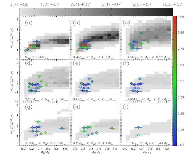
Figure 2: Calculated present-day PCEB populations, for model A and for $n(q_{\mathrm{i}})=1$. The distributions over $M_{2}$ and $\mathrm{log}P_{\mathrm{orb}}$ are shown for nine different white dwarf mass intervals as indicated in each of the nine panels, labelled (a) to (i). The grey-scale bar at the top of the plot indicates the number of systems per bin area. Also shown are the known WD+MS systems obtained from Edition 7.10 (2008) of RKCat (Ritter & Kolb, 2003). We take into account the uncertainties of the white dwarf mass for each system by calculating the weighting of each system within each panel. This is repeated for those systems whose error bars in white dwarf mass overlaps more than one panel. The weighting is indicated by the colour bar on the right hand side of the plot. The dotted line in panel (b) indicates that the secondary mass in SDSS J1724+5620 lies between 0.25 M_⊙ and 0.38 M_⊙.

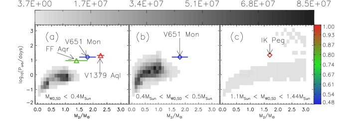
Figure 3: The theoretical present day PCEB population for model A, $n(q_{\mathrm{i}})=1$, for a wider range in $M_{2}$ and $P_{\mathrm{orb}}$ than Fig. 2, for selected white dwarf mass intervals. Each panel labelled (a) to (c) represents the indicated range in white dwarf or sub-dwarf mass. Diamonds: WD+MS systems; triangles: sd+MS systems. The location of the individual systems V651 Mon, V1379 Aql and FF Aqr are indicated by the arrows. The grey-scale on the top of the plot indicates the number of systems per bin area, while the bar on the right hand side indicates the weighting of the systems in their corresponding panels.

Both the theoretical distributions and observed systems are divided into panels according to their white dwarf masses as indicated in each of the nine panels, labelled (a) to (i). The grey-scale bar at the top of the plot indicates the number of systems per bin area. We take into account the uncertainty of the white dwarf masses for each observed system by calculating the weighting of the system in each panel that overlaps with the white dwarf uncertainty interval. The panels in which these systems lie, and the associated weightings, are also shown in Table LABEL:table01. The weightings are calculated from a Gaussian distribution with a mean white dwarf mass $\langle{M_{\mathrm{WD}}}\rangle$ and a standard deviation $\sigma$, which corresponds to the measured white dwarf mass and its uncertainty respectively. The colour bar on the right hand side of the plot indicates the weightings.

There is an acceptable overall agreement between the observed systems and the theoretical distributions, in the sense that all but two observed systems are in areas populated by the standard model. However, the model distributions extend to areas at orbital periods longer than about 1 d and donor masses larger than about 0.5 M_⊙ with very few, if any, observed systems. The two outliers that cannot be accounted for by our standard model are V651 Mon (Mendez & Niemela 1981; Mendez et al. 1985; Kato, Nogami & Baba 2001) and IK Peg (Vennes, Christian & Thorstensen 1998). The location of these systems are indicated in Figure 3 by the arrows (these systems lie outside of the range displayed in Figure 2 and so are not shown there). We shall discuss these systems in turn to deduce whether they are in fact PCEBs.

IK Peg contains a $1.2$ M_⊙ white dwarf, and a $1.7$ M_⊙ secondary star with spectral type A8 (Landsman, Simon & Bergeron 1993; Smalley et al. 1996; Vennes, Christian & Thorstensen 1998). Smalley et al. (1996) found that the secondary star had an overabundance of iron, barium and strontium, which may be accounted for if IK Peg underwent mass transfer. Smalley et al. (1996) suggest that this was in the form of a CE phase. As the secondary plunged into the envelope of the giant it would be contaminated by s-processed material. As WD+MS systems can also form through a thermally unstable Roche lobe overflow (RLOF) phase (see Willems & Kolb 2004, formation channels 1 to 3), we calculated the present day population of WD+MS systems with $1.1\leq{M_{\mathrm{WD}}/\mathrm{M}_{\odot}}\leq{1.44}$ that form through such a case B thermal–timescale mass transfer (TTMT) phase (channel 2 in Willems & Kolb 2004), which is shown in the right panel of Figure 4. The diamond indicates the location of IK Peg. As the location of IK Peg cannot be accounted for by our theoretical population of case B TTMT systems, it is hence a likely PCEB candidate. We explore this possibility further in Section 3.5 where we consider more population synthesis models of the CE phase.

V651 Mon contains a 0.4 M_⊙ hot white dwarf primary with an A-type secondary star. This system lies within a planetary nebula, which could be the remnant of a CE phase. However, de Kool & Ritter (1993) suggest that the planetary nebula may have formed when the compact primary underwent a shell flash, and instead the binary formed via a thermally unstable RLOF phase. As for IK Peg, we calculate the present day population of WD+MS systems with $M_{\mathrm{WD}}/\mathrm{M}_{\odot}\leq{0.4}$ that formed through a thermally unstable RLOF phase, shown in the left panel of Figure 4. This is compared with the location of V651 Mon shown as indicated by the arrow. From Figure 4 it appears hence feasible that V651 Mon formed from a case B RLOF phase.

To obtain the possible progenitor of V651 Mon, we first find the calculated WD+MS configuration which formed through the case B TTMT channel which is situated closest to the location of V651 Mon in $(M_{\mathrm{WD}},M_{2},P_{\mathrm{orb}})$ space. If $\delta{M_{\mathrm{WD}}}$, $\delta{M_{2}}$ and $\delta{P_{\mathrm{orb}}}$ is the difference between the observed white dwarf mass $M_{\mathrm{WD,obs}}$, secondary mass $M_{2,\mathrm{obs}}$ and orbital period $P_{\mathrm{orb,obs}}$ of V651 Mon and a calculated WD+MS binary configuration, then the normalised distance, $\Delta$, in $(M_{\mathrm{WD}},M_{2},P_{\mathrm{orb}})$ space is given by

$$\Delta=\left(\left|\frac{\delta{M_{\mathrm{WD}}}}{M_{\mathrm{WD,obs}}}\right|^{2}+\left|\frac{\delta{M_{2}}}{M_{2,\mathrm{obs}}}\right|^{2}+\left|\frac{\delta{P_{\mathrm{orb}}}}{P_{\mathrm{orb,obs}}}\right|^{2}\right)^{1/2}$$ (13)

Thus we require the WD+MS binary configuration that gives the smallest value of $\Delta$. We find that $\Delta$ is minimised for $M_{\mathrm{WD}}=0.33$ M_⊙, $M_{2}=1.76$ M_⊙ and $P_{\mathrm{orb}}=15.92$ d. This system has a ZAMS progenitor with $M_{1,\mathrm{i}}=2.47$ M_⊙, $M_{2,\mathrm{i}}=0.98$ M_⊙ and $P_{\mathrm{orb,i}}=2.60$ d.

While the secondary mass of this WD+MS configuration is within the measured uncertainty of the secondary mass in V651 Mon, its white dwarf mass is not, and in fact underestimates the white dwarf mass of V651 Mon. Tout & Eggleton (1988) and Tout & Eggleton (1988b) suggest that V651 Mon may have formed with enhanced mass loss from the primary star before it filled its Roche lobe. Thus, a more massive progenitor primary than the one found in our best-fit WD+MS configuration may have formed the white dwarf. If enough mass is lost from the primary due to enhanced wind losses before it fills its Roche lobe to sufficiently lower the mass ratio, $M_{1}/M_{2}$, then the resulting mass transfer will be dynamically stable.

3.2 Sub-dwarf + main sequence star binaries

One of the main formation channels of sd+MS binaries is via the CE phase (Han et al., 2002); if the primary star fills its Roche lobe near the tip of the first giant branch, and the CE is ejected from the system, then a short-period binary with an sd star is formed once the helium core is ignited. Han et al. (2002) found that the mass of the sdB star ranges from approximately 0.32 to 0.48 $M_{\odot}$. The typical mass for a sdB star is approximately 0.46 M_⊙. This appears to be broadly consistent with the observed masses of sd stars (see Table LABEL:table02). The mass of the sub-dwarf in V1379 Aql is somewhat smaller than the calculated lower limit by Han et al. (2002), while the sub-dwarfs in UU Sge and KV Kel are more massive than the calculated upper limit in sub-dwarf mass.

The formation of sub-dwarf stars is affected by the wind loss of the giant’s envelope, the metallicity of the primary, and the degree of convective overshooting of the primary. A detailed consideration of sdB binaries is beyond the scope of this study. Instead, we simply plot the observed sample of sd+MS binaries over our calculated distributions of the WD+MS PCEBs (see Figure 5, for model A and $n(q_{\mathrm{i}})=1$, in the same style as Figure 2), thereby assuming that there is little orbital evolution of these systems by the time the sdB stars become white dwarfs. This is justified as follows:

The evolution of sd+MS binaries will be driven by wind losses from the subdwarf primary with a mass loss rate of approximately ${10}^{-11}$ M_⊙ yr^-1 (Vink (2004); Unglaub (2008)), as well as systemic angular momentum losses. For the observed sample of sd+MS systems in Table LABEL:table02, $M_{2}<0.35$ M_⊙ in all cases, and so gravitational wave radiation will therefore be the only sink of orbital angular momentum. During the lifetime of an sdB (i.e. the core helium burning time) of approximately few$\times{10^{8}}$ yr (Hurley, Pols & Tout, 2000), we estimate a relative change in the binary’s orbital period of less than about 7 per cent.

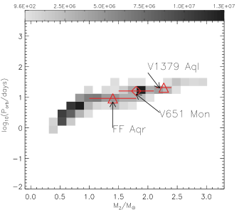
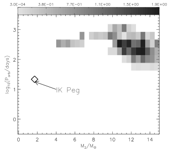
Figure 4: Left panel: The theoretical population of WD+MS systems with $M_{\mathrm{WD}}/\mathrm{M}_{\odot}\leq{0.4}$ that formed through a thermally unstable RLOF phase, compared with the location of FF Aqr, V651 Mon, and V1379 Aql, as indicated by the arrows. Right panel: The theoretical population of WD+MS systems with $1.1\leq{M_{\mathrm{WD}}/\mathrm{M}_{\odot}}\leq{1.44}$ that formed through a thermally unstable RLOF phase with a naked helium star remnant. This is compared with the location of IK Peg indicated by the arrow. A triangular symbol indicates that the system is a sd+MS binary, while a diamond indicates the system is a WD+MS binary.

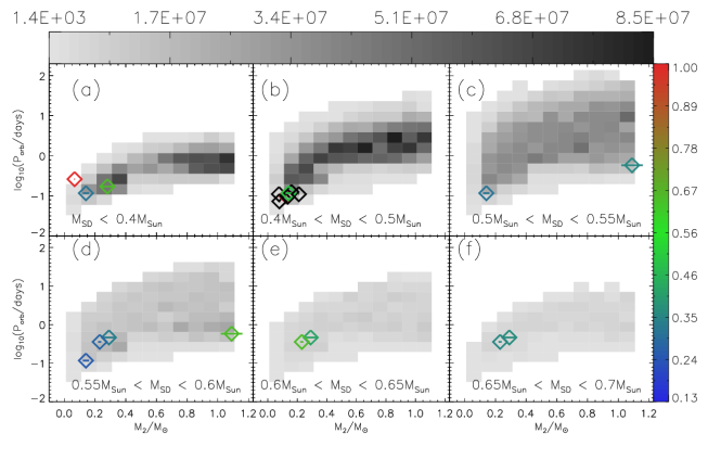
Figure 5: Same as Figure 2 but this time showing the observed sample of sub-dwarf+MS binaries. The black points represent those systems for which we have not calculated the weightings, as measured uncertainties for the sub-dwarf masses are not available.

Figure 5 shows that, as with the observed WD+MS systems, there are observed sd+MS systems that cannot be explained by our standard model. These are FF Aqr and V1379 Aql. Their locations are indicated in the left panel of Figure 3 by the arrows. We discuss these systems individually to determine whether they are in fact PCEBs.

V1379 Aql This system contains a K-giant secondary and an sdB primary, which may be a nascent helium white dwarf (Jeffery, Simon & Evans, 1992). Furthermore, Jeffery & Simon (1997) argue that V1379 Aql formed from a thermally unstable RLOF phase. As a consequence of the synchronous rotation of the secondary, the system exhibits RS CVn chromospheric activity due to the K-giant’s enhanced magnetic activity. This is likely to occur if the system had a previous episode of RLOF, rather than if the system has emerged from a CE phase.

Tout & Eggleton (1988b) suggest that the progenitor binary of V1379 Aql had $M_{1,\mathrm{i}}=2.0$ M_⊙ and $M_{2,\mathrm{i}}=1.6$ M_⊙. The secondary star would have completed one half of its main sequence lifetime by the time the primary evolved to become a giant after approximately ${6}\times{10}^{8}$ yr (Jeffery, Simon & Evans, 1992). If a CE phase did occur, then the secondary would still have been on the main sequence, and hence possess an insubstantial convective envelope. Consequently, magnetic braking would be ineffective in shrinking the orbital separation sufficiently for tidal interactions to enforce synchronous rotation of the secondary star.

Nelemans & Tout (2005), in reconstructing a possible CE phase for this system, could not find a solution for $\alpha_{\mathrm{CE}}$, and cited this as evidence for their alternative CE description in terms of the angular momentum balance. We suggest that no solution was found because of the possibility that V1379 Aql formed from a thermally unstable RLOF phase.

The left panel of Figure 4 compares the theoretical WD+MS systems with $M_{\mathrm{WD}}/\mathrm{M}_{\odot}\leq{0.4}$ that formed through a thermally unstable RLOF phase with the location of V1379 Aql shown by the arrow. It appears hence feasible that V1379 Aql formed through this evolutionary channel. As with V651 Mon, we apply equation (13) to find the WD+MS configuration which lies the closest to the location of V1379 Aql in $(M_{\mathrm{WD}},M_{2},P_{\mathrm{orb}})$. Doing this we find a WD+MS configuration with $M_{\mathrm{WD}}=0.23$ M_⊙, $M_{2}=2.31$ M_⊙ and $P_{\mathrm{orb}}=20.58$ d. This system forms from a ZAMS progenitor with $M_{1,\mathrm{i}}=1.79$ M_⊙, $M_{2,\mathrm{i}}=0.77$ M_⊙ and $P_{\mathrm{orb,i}}=1.41$ d.

The mass of the white dwarf in our best-fit WD+MS configuration once again underestimates that of V1379 Aql. As for V651 Mon,Tout & Eggleton (1988b) suggest that the primary star in V1379 Aql also underwent enhanced mass loss before it filled its Roche lobe. Thus, the mass ratio, $M_{1}/M_{2}$, was decreased sufficiently so that a dynamically unstable RLOF phase was avoided. The actual progenitor primary of V1379 Aql may therefore have been more massive than what we have predicted in our calculations. Note also that in our calculations, we do not treat the sdB phase of the white dwarf explicitly.

FF Aqr also displays RS CVn characteristics (Vaccaro & Wilson, 2003), and hence we can apply the same argument used for V1379 Aql to FF Aqr; the secondary has a mass of approximately 1.4 M_⊙ and so will have an insubstantial convective envelope. Indeed, de Kool & Ritter (1993) argue that FF Aqr formed from a thermally unstable RLOF phase, perhaps with enhanced wind losses (Tout & Eggleton, 1988b).

The left panel of Figure 4, compares the theoretical WD+MS binary population with $M_{\mathrm{WD}}/\mathrm{M}_{\odot}\leq{0.4}$, which formed through a channel 1 Willems & Kolb (2004) RLOF phase, with the location of FF Aqr indicated by the arrow. This supports the possibility that FF Aqr formed from a TTMT RLOF phase. While our best fit WD+MS configuration has $M_{\mathrm{WD}}=0.30$ M_⊙, which is consistent with the observed value within the measured uncertainty, our best-fit configuration slightly underestimates the secondary mass with $M_{2}=1.22$ M_⊙.

3.3 The shape of the distributions

Figure 6: Critical boundaries in the $\mathrm{log}_{10}(P_{\mathrm{orb}})-M_{2}$ plane. The long dashed line shows the upper boundary in the population of progenitor binaries at the start of the CE phase which will form PCEBs with $0.4<M_{\mathrm{WD}}/\mathrm{M}_{\odot}\leq{0.5}$. The values along this line denote the mass of the Roche lobe-filling progenitor primary at the corresponding locations along the boundary. The short dashed line is the upper boundary in the resulting population of PCEBs with $0.4<M_{\mathrm{WD}}\leq{0.5}$. The values along this line denote the white dwarf mass The label ‘A’ corresponds to the portion of the boundary at $M_{2}\la{1.1}$ M_⊙ (short-dashed line), while ‘B’ denotes the portion of the boundary at $M_{2}\ga{1.1}$ M_⊙. The thick black line is the Roche lobe-overflow (RLOF) limit, i.e. the point at which the PCEB will become semi-detached, and hence defines the lower limit in the distribution. Finally, the dot-dashed line corresponds to the cut-off in this PCEB population at $M_{2}\approx{1.8}$ M_⊙.

We will now discuss common features of the $M_{2}-\mathrm{log_{10}}P_{\mathrm{orb}}$ PCEB distributions, with the middle panel of Figure 3 as a typical example.

Figure 6 shows the upper boundary in the population of progenitor systems at the onset of the CE phase which will form PCEBs with $0.4<M_{\mathrm{WD}}/\mathrm{M}_{\odot}\leq{0.5}$ (long dashed line). The short dashed line shows the corresponding upper boundary in the resulting population of PCEBs (this represents the upper boundary of the distribution shown in the middle panel of Figure 3), while the thick, black line shows the orbital period at which the secondary star will undergo Roche lobe overflow (RLOF), and hence the PCEB will become semi-detached.

The long dashed boundary in Figure 6 arises because for each mass $M_{2}$ there is an upper limit for the orbital period of the progenitor binary that will still form a white dwarf with a mass within the considered mass interval. Longer-period systems will either form a more massive white dwarf, or remain detached and not undergo a CE phase. More specifically, the upper boundary corresponds to the most massive white dwarfs in the panel. In the example shown this is 0.47 M_⊙ (not 0.50 M_⊙) because there is a gap in the white dwarf mass spectrum between the low-mass helium white dwarfs and the more massive carbon-oxygen white dwarfs. The SSE code (Hurley, Pols & Tout, 2000) places this gap in the range between $0.47<M_{\mathrm{WD}}/\mathrm{M}_{\odot}<0.6$.

This long dashed upper pre-CE boundary maps on to the short dashed PCEB boundary, also shown in Figure 6. The masses of the progenitor primaries at the start of the CE phase are indicated along the long-dashed boundary, while the white dwarf masses are shown along the short-dashed boundary of the PCEB population, at the corresponding point along the boundary.

For a PCEB to form, the ZAMS progenitor primary must fill its Roche lobe and commence the CE phase before the secondary itself evolves off the main sequence. This point is of little consequence for $M_{2,\mathrm{i}}\la{1}$ M_⊙ as the main sequence lifetime of such secondaries will be $\tau_{\mathrm{MS,2}}\ga{10}$ Gyr, which is on the order of the Galactic lifetime (and the maximum evolution time we consider). Thus, in such cases, the progenitor primary must ascend the giant branch and fill its Roche lobe within the lifetime of the Galaxy.

We find that the least massive ZAMS progenitor which will subsequently form a 0.47 M_⊙ white dwarf within the lifetime of the Galaxy, is 1.1 M_⊙. Hence, for the reasons stated above, $M_{2,\mathrm{i}}<1.1$ M_⊙, if the evolution of the secondary off the main sequence is to remain unimportant. As indicated along the long-dashed boundary in Figure 6 for $M_{2}<1.1$ M_⊙(to the left of the dashed vertical line), the progenitor primaries, as a result of wind losses, commence the CE phase with masses of approximately 0.9 M_⊙. Furthermore, as the long-dashed boundary for $M_{2}<1.1$ M_⊙ is approximately flat, the progenitor primaries along this boundary fill their Roche lobes at the same orbital period.

To see how this determines the shape of the resulting short-dashed PCEB boundary for $M_{2}<1.1$ M_⊙ (labelled ‘A’ in Figure 6) we consider equation (5), which shows that for constant $M_{\mathrm{c}}$ (and hence the white dwarf mass), $M_{1}$ and $r_{\mathrm{L,1}}$ (at the start of the CE phase), $A_{\mathrm{CE,f}}$ decreases for decreasing $M_{2}$. Hence the orbital period of the short-dashed boundary to the left of the dashed line in Figure 6 decreases for decreasing $M_{2}$.

On the other hand, for $M_{2,\mathrm{i}}>1.1$ M_⊙ (to the right of the dashed line in Figure 6), the main sequence lifetime of such stars is less than 10 Gyr, and so the progenitor primary must increasingly compete against the secondary to evolve off the main sequence first. As a result, the ZAMS progenitor primary star needs to be increasingly more massive for increasing secondary mass. This is reflected in the masses of the primaries at the start of the CE phase, as indicated along the long-dashed boundary in Figure 6 for $M_{2}>1.1$ M_⊙, which increase from approximately 0.9 M_⊙ where $M_{2}\approx{1.1}$ M_⊙, to 1.8 M_⊙ where $M_{2}\approx{1.8}$ M_⊙.

For a primary star ascending the giant branch with luminosity $L_{1}$, its radius on the giant branch, $R_{\mathrm{GB}}$, can be modelled as

$$R_{\mathrm{GB}}\approx\frac{1.1}{M_{1,\mathrm{i}}^{0.3}}\left(L_{1}^{0.4}+0.383L_{1}^{0.76}\right),$$ (14)

(Hurley, Pols & Tout, 2000), where $L_{1}\propto{M_{\mathrm{c}}}^{6}$. Thus the radius of the star on the giant branch is a function of its core mass and (weakly) of its initial ZAMS mass. For a given core mass, in this case of $M_{\mathrm{c}}=0.47$ M_⊙, the corresponding value of $R_{\mathrm{GB}}$ will decrease for increasing mass of the ZAMS primary. For Roche lobe filling stars we have $P_{\mathrm{orb}}\propto{R}^{3/2}/M^{1/2}$ so the orbital period at which the CE phase will occur will decrease with increasing $M_{2}$. This is shown as the slope in the long-dashed boundary in Figure 6 for $M_{2}>1.1$ M_⊙.

The shape of the short-dashed boundary to the right of the dashed line in Figure 6 (labelled ‘B’) is a consequence of the shape of the corresponding portion of the long-dashed pre-CE boundary. Furthermore, for increasing $M_{2}$, while M_c remains constant, $M_{\mathrm{1,i}}$ does increase, and so the mass of the primary giant’s envelope will correspondingly increase. The result of this is that $A_{\mathrm{CE,f}}$ will decrease for increasing $M_{2}$, as equation (5) shows. This explains why the short-dashed PCEB boundary to the right of the dashed lin Figure 6 decreasing for increasing $M_{2}$.

Note that the cut-off in the population, as indicated by the vertical dot-dashed line (at $M_{2}\approx{1.8}$ M_⊙) in Figure 6, is a consequence of the fact that the most massive progenitor primary which will form a white dwarf in the range $0.4<M_{\mathrm{WD}}/\mathrm{M}_{\odot}\leq{0.5}$ is 1.8 M_⊙. For PCEB distributions with larger white dwarf masses, which will be formed from more massive primary progenitors, this cut-off will shift towards larger values of $M_{2}$.

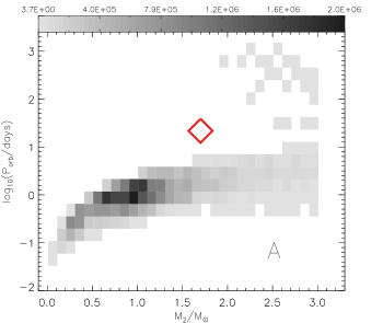
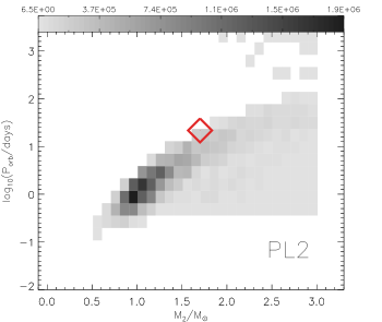
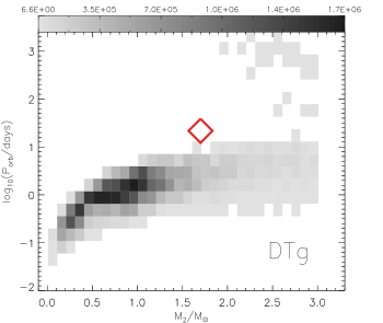
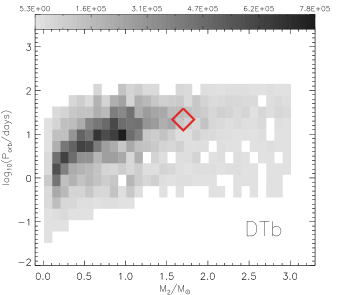
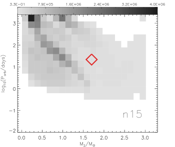
Figure 7: Calculated PCEB populations with $1.1<M_{\mathrm{WD}}/\mathrm{M}_{\odot}\leq{1.44}$ for a range of models indicated in the lower right hand corner of each plot. Here $n(q_{\mathrm{i}})=1$. The observed location of IK Peg is indicated by a diamond. The grey-scale bars above each plot indicates the number of systems per bin area.

3.4 The present day population and space densities of PCEBs

Table LABEL:table_stats summarises the formation rate, present day population and the local space density, $\varrho$, of PCEBs for each model describing the treatment of the CE phase, and for each population model we considered. We calculate the local space density of PCEBs by dividing the present day population by the Galactic volume of $5\times{10}^{11}$ pc³.

For a given initial secondary mass distribution, we see that the present day population of PCEBs increases with increasing values of $\alpha_{\mathrm{CE}}$. By increasing $\alpha_{\mathrm{CE}}$, less orbital energy is required to eject the CE and therefore the binary system will undergo less spiral in. Hence, fewer systems will merge during the CE phase. For a given IMRD, we find very little difference in the calculated formation rates, present day numbers and local space densities of PCEBs between models A and DTg. For model DTb, on the other hand, where we are now considering the internal energy of the giant’s envelope, we obtain a modest increase in the present day population of PCEBs compared to model A.

The present day population of PCEBs decreases slightly with increasing values of $p$ in equation (6). As shown in Figure 1 of Politano & Weiler (2007) the average value of $\alpha_{\mathrm{CE}}$ for a given range in $M_{2}$ decreases with increasing $p$. By increasing $p$ more orbital energy is required to expel the envelope from the system, hence a larger spiral-in of the binary. This will in turn lead to more mergers.

On the other hand, the present day number (local space density) of PCEBs decreases from model CT0375 to model CT15. As we increase the value of $M_{\mathrm{cut}}$ the typical value of $\alpha_{\mathrm{CE}}$ for a given range of $M_{2}$ will decrease. Hence, fewer systems will survive the CE phase.

We notice that the model n15 which describes the CE phase in terms of the binary’s angular momentum gives the largest present day population of PCEBs. For $n(q_{\mathrm{i}})=1$, the present day number (local space density) of PCEBs is $6.1\times{10}^{8}$ ($1.2\times{10}^{-3}$ pc^-3).

Schreiber & Gänsicke (2003) estimated from the observed sample of PCEBs that $6\times{10}^{-6}\la{\varrho}/\mathrm{pc}^{-3}\la{3\times{10}^{-5}}$. An IMRD of $n(q_{\mathrm{i}})\propto{q_{\mathrm{i}}}^{-0.99}$ gives the best agreement with this observed estimate, where we obtain $6.0\times{10}^{-7}\leq{\varrho}/\mathrm{pc}^{-3}\leq{5.6\times{10}^{-5}}$.

Our models with $\alpha_{\mathrm{CE}}=0.1$ also provide small space densities ($6.0\times{10}^{-7}\leq{\varrho/\mathrm{pc}^{-3}}\leq{1.7\times{10}^{-5}}$, depending on the IMRD), which are similar to the observed ones. However, we find that in these models no PCEBs with M${}_{\mathrm{WD}}/\mathrm{M_{\odot}}\leq{0.4}$ form. Low mass helium white dwarfs form via a case B CE phase, when the primary fills its Roche lobe on the first giant branch, typically when $R_{1}\approx{15}$ to 100 R_⊙. This means that the orbital period at the onset of the CE phase is between approximately 40 and 250 d. As a consequence of such a low ejection efficiency, the binary cannot spiral in sufficiently to eject the envelope before a merger occurs. The lack of PCEBs with low mass white dwarfs in models with $\alpha_{\mathrm{CE}}=0.1$ is in conflict with observations; for example LM Com and 0137-3457 have 95 per cent and 61 per cent probabilities respectively of having $M_{\mathrm{WD}}/\mathrm{M}_{\odot}\leq{0.4}$.

Table 4: The formation rates, present day numbers and local space densities of PCEBs for different treatments of the CE phase, and for different initial mass distributions of the secondary star. The space densities were calculated by dividing the present day numbers by the Galactic volume of $5\times{10}^{11}$ pc³.

Model	Formation rate	Number of systems	Local space
	/yr-1		density /pc-3
$n(q_{\mathrm{i}})\propto{q_{\mathrm{i}}^{-0.99}}$, $0<q_{\mathrm{i}}\leq{1}$
CE01	$2.1\times{10}^{-4}$	$3.0\times{10}^{5}$	$6.0\times{10}^{-7}$
CE06	$1.5\times{10}^{-3}$	$4.4\times{10}^{6}$	$8.8\times{10}^{-6}$
A	$2.0\times{10}^{-3}$	$7.3\times{10}^{6}$	$1.5\times{10}^{-5}$
PL05	$1.6\times{10}^{-3}$	$4.8\times{10}^{6}$	$9.6\times{10}^{-6}$
PL1	$1.3\times{10}^{-3}$	$3.6\times{10}^{6}$	$7.2\times{10}^{-6}$
PL2	$1.1\times{10}^{-3}$	$2.7\times{10}^{6}$	$5.4\times{10}^{-6}$
CT0375	$1.8\times{10}^{-3}$	$6.6\times{10}^{6}$	$1.3\times{10}^{-5}$
CT075	$1.7\times{10}^{-3}$	$5.7\times{10}^{6}$	$1.1\times{10}^{-5}$
CT15	$1.3\times{10}^{-3}$	$4.2\times{10}^{6}$	$8.5\times{10}^{-6}$
DTg	$1.9\times{10}^{-3}$	$6.8\times{10}^{6}$	$1.3\times{10}^{-5}$
DTb	$2.5\times{10}^{-3}$	$1.2\times{10}^{7}$	$2.4\times{10}^{-5}$
n15	$5.4\times{10}^{-3}$	$2.8\times{10}^{7}$	$5.6\times{10}^{-5}$
$n(q_{\mathrm{i}})=1$, $0<q_{\mathrm{i}}\leq{1}$ (our reference IMRD)
CE01	$9.8\times{10}^{-3}$	$1.5\times{10}^{7}$	$3.0\times{10}^{-5}$
CE06	$5.5\times{10}^{-2}$	$1.5\times{10}^{8}$	$3.0\times{10}^{-4}$
A	$7.2\times{10}^{-2}$	$2.2\times{10}^{8}$	$4.4\times{10}^{-4}$
PL05	$6.8\times{10}^{-2}$	$1.9\times{10}^{8}$	$3.8\times{10}^{-4}$
PL1	$6.5\times{10}^{-2}$	$1.6\times{10}^{8}$	$3.2\times{10}^{-4}$
PL2	$6.1\times{10}^{-2}$	$1.4\times{10}^{8}$	$2.8\times{10}^{-4}$
CT0375	$7.0\times{10}^{-2}$	$2.1\times{10}^{8}$	$4.3\times{10}^{-4}$
CT075	$6.7\times{10}^{-2}$	$2.0\times{10}^{8}$	$4.0\times{10}^{-4}$
CT15	$6.0\times{10}^{-2}$	$1.7\times{10}^{8}$	$3.5\times{10}^{-4}$
DTg	$7.0\times{10}^{-2}$	$2.0\times{10}^{8}$	$4.0\times{10}^{-4}$
DTb	$8.7\times{10}^{-2}$	$3.1\times{10}^{8}$	$6.2\times{10}^{-4}$
n15	$3.6\times{10}^{-1}$	$6.1\times{10}^{8}$	$1.2\times{10}^{-3}$
$n(q_{\mathrm{i}})\propto{q_{\mathrm{i}}}$, $0<q_{\mathrm{i}}\leq{1}$
CE01	$1.1\times{10}^{-2}$	$1.9\times{10}^{7}$	$3.8\times{10}^{-5}$
CE06	$5.8\times{10}^{-2}$	$1.4\times{10}^{8}$	$2.8\times{10}^{-4}$
A	$7.5\times{10}^{-2}$	$2.0\times{10}^{8}$	$4.0\times{10}^{-4}$
PL05	$7.7\times{10}^{-2}$	$1.8\times{10}^{8}$	$3.6\times{10}^{-4}$
PL1	$7.8\times{10}^{-2}$	$1.8\times{10}^{8}$	$3.6\times{10}^{-4}$
PL2	$7.8\times{10}^{-2}$	$1.6\times{10}^{8}$	$3.2\times{10}^{-4}$
CT0375	$7.3\times{10}^{-2}$	$2.0\times{10}^{8}$	$3.9\times{10}^{-4}$
CT075	$7.2\times{10}^{-2}$	$1.9\times{10}^{8}$	$3.8\times{10}^{-4}$
CT15	$6.8\times{10}^{-2}$	$1.7\times{10}^{8}$	$3.5\times{10}^{-4}$
DTg	$7.3\times{10}^{-2}$	$1.8\times{10}^{8}$	$3.6\times{10}^{-4}$
DTb	$9.0\times{10}^{-2}$	$2.7\times{10}^{8}$	$5.4\times{10}^{-4}$
n15	$1.7\times{10}^{-1}$	$4.9\times{10}^{8}$	$9.8\times{10}^{-4}$
IMFM2
CE01	$6.5\times{10}^{-3}$	$8.3\times{10}^{6}$	$1.7\times{10}^{-5}$
CE06	$4.7\times{10}^{-2}$	$1.5\times{10}^{8}$	$3.0\times{10}^{-4}$
A	$6.5\times{10}^{-2}$	$2.5\times{10}^{8}$	$5.0\times{10}^{-4}$
PL05	$4.4\times{10}^{-2}$	$1.4\times{10}^{8}$	$2.8\times{10}^{-4}$
PL1	$3.0\times{10}^{-2}$	$8.3\times{10}^{7}$	$1.7\times{10}^{-4}$
PL2	$1.7\times{10}^{-2}$	$4.7\times{10}^{7}$	$9.4\times{10}^{-5}$
CT0375	$5.8\times{10}^{-2}$	$2.2\times{10}^{8}$	$4.4\times{10}^{-4}$
CT075	$4.9\times{10}^{-2}$	$1.8\times{10}^{8}$	$3.5\times{10}^{-4}$
CT15	$3.3\times{10}^{-2}$	$1.1\times{10}^{8}$	$2.2\times{10}^{-4}$
DTg	$6.1\times{10}^{-2}$	$2.3\times{10}^{8}$	$4.6\times{10}^{-4}$
DTb	$8.5\times{10}^{-2}$	$4.2\times{10}^{8}$	$8.4\times{10}^{-4}$
n15	$1.9\times{10}^{-1}$	$1.1\times{10}^{9}$	$2.2\times{10}^{-3}$

3.5 IK Peg: A Clue to the CE Mechanism?

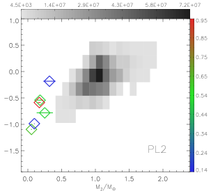
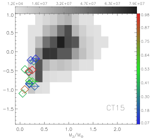
Figure 8: Same as for Fig. 2 but now showing the theoretical and observed PCEB population with $M_{\mathrm{WD}}/\mathrm{M}_{\odot}\leq{0.4}$ for model PL2 (top panel) and for model CT15 (bottom panel); in both cases $n(q_{\mathrm{i}})=1$. The grey-scale bar above the plots indicates the number of systems per bin area, while the bar on the right indicates the weightings of the observed systems.

As discussed above, the bulk of observed systems which have $M_{2}/\mathrm{M}_{\odot}\la{1.0}$ and $P_{\mathrm{orb}}/\mathrm{d}\la{1}$ are consistent with our reference model A. IK Peg, on the other hand, cannot be explained by models with $\alpha_{\mathrm{CE}}\leq{1.0}$, for $\lambda=0.5$. Figure 7 shows the theoretical PCEB population with $1.1<M_{\mathrm{WD}}/\mathrm{M}_{\odot}\leq{1.44}$ for a range of models, indicated in the bottom right hand corner of each panel. The location of IK Peg on the $M_{2}-\mathrm{log}\,P_{\mathrm{orb}}$ plane is indicated as the diamond in each case.

In order to explain the location of IK Peg, we require $\alpha_{\mathrm{CE}}\ga{3}$, if $\lambda=0.5$. Model PL2 achieves $\alpha_{\mathrm{CE}}\approx{2.9}$ for this system and, as shown in the panel labelled ‘PL2’ in Figure 7 can account for the location of IK Peg. However, this model also generates a low-mass cut-off at $M_{2}\approx{0.4}$ M_⊙ in the PCEB population. This is a feature which is not consistent with observed systems, as highlighted in the top panel of Figure 8. LM Com and 0137-3457 have a 95 per cent and a 61 per cent probability of sitting in this panel. Thus it appears this model cannot adequately describe the CE phase in its present form.

Note that models CT0375 to CT15 cannot account for the location of IK Peg either. From equation (7) $\alpha_{\mathrm{CE}}\rightarrow{1}$ as $M_{2}\rightarrow{\infty}$. As with the model PL2, the cut-off (by design of the model) in the PCEB population at $M_{2}=0.15$ M_⊙ doesn’t appear to be supported by the observed sample. The bottom panel of Figure 8 compares the theoretical PCEB population with $0.4<M_{\mathrm{WD}}/\mathrm{M}_{\odot}\leq{0.5}$, with the corresponding observed WD+MS systems. Indeed, model CT15 cannot account for the observed location of, for example, HR Cam or 0137-3457, which have a 84 and 61 per cent probability of occupying this panel.

Model DTb, where the thermal energy of the giant’s envelope contributes to the ejection of the CE, can also account for the location of IK Peg, while DTg cannot (see panels labelled ‘DTb’ and DTg’ in Figure 7). Model DTg shows a slight increase in the orbital period of the upper boundary in the theoretical PCEB population, compared to that shown in the panel labelled ‘A’, but this is not enough to account for IK Peg. A possible primary progenitor of IK Peg would fill its Roche lobe with a mass of 6 M_⊙ and a radius of 725 R_⊙. From Fig. 1 (dashed line), we find $\lambda_{\mathrm{g}}\approx{0.6}$. However, to account for the location of IK Peg, we require $\lambda_{\mathrm{g}}\approx{2.2}$ (with $\alpha_{\mathrm{CE}}=1$).

Finally, the location of IK Peg can be accounted for if we consider an angular momentum, rather than an energy, budget, as shown by the panel ‘n15’. Of further interest is that, in contrast to the other models considered in Figure 9, model n15 predicts no PCEBs with $M_{2}\la{1.0}$ M_⊙ at $P_{\mathrm{orb}}\la{1}$ d. Furthermore, while the PCEB population in models A to DTb peaks at $P_{\mathrm{orb}}\approx{1}$ to 10 d, the model n15 population peaks at $P_{\mathrm{orb}}\approx{1000}$ d. This confirms the result by Maxted et al. (2007).

3.6 The Initial Secondary mass Distribution

We now consider the impact of the initial mass ratio distribution on the theoretical PCEB populations. For our standard model A we calculated the PCEB population for each initial distribution of the secondary mass, which we compared to the observed WD+MS systems. Figure 9 illustrates the differences between the resulting PCEB populations in the range $0.4<M_{\mathrm{WD}}/\mathrm{M_{\odot}}\leq{0.5}$ as an example.

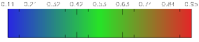
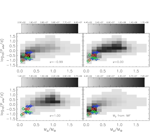
Figure 9: Same as Fig. 2, but showing the population of PCEBs with $0.4<M_{\mathrm{WD}}/\mathrm{M}_{\odot}\leq{0.5}$ for different initial secondary mass distributions, as indicated in each panel. The grey-scale bar above each panel gives the number of systems per bin area, while the colour bar at the top of the page gives the weighting of each system.

For the cases $n(q_{\mathrm{i}})\propto{q_{\mathrm{i}}}^{-0.99}$ and IMFM2 the bulk of the PCEB population lies at $M_{2}\la{0.4}$ M_⊙ and $P_{\mathrm{orb}}\la{1}$ d. This is consistent with the location of the observed WD+MS systems in Figure 9. The theoretical distribution with $n(q_{\mathrm{i}})=1$ suggests a peak at $M_{2}\approx{1}$ M_⊙ and $P_{\mathrm{orb}}\approx{1}$ d, yet no systems are observed in this region of $M_{2}-\mathrm{log}\,P_{\mathrm{orb}}$ space. However, this is likely to be a selection effect; PCEB candidates are selected according to their blue colour due to the optical emission from the white dwarf and/or high radial velocity variations. The flux from early-type secondaries will dominate over that of the white dwarf, and hence these systems go undetected. Schreiber & Gänsicke (2003) predicted that there is a large as yet undetected population of old PCEBs, with cool white dwarfs and long orbital period.

Rebassa-Mansergas et al. (2008) performed Monte-Carlo simulations to calculate the detection probability of PCEBs with $P_{\mathrm{orb}}/\mathrm{d}\la{10}$, based on the measurement accuracies of the Very Large Telescope (Schreiber et al., 2008), the SDSS, and for 1, 2 and $3\sigma$ significance of the radial velocity variations. They found that approximately 6 out of their sample of 9 PCEBs should have $P_{\mathrm{orb}}>1$ d, yet this is not the case; all of their PCEBs have $P_{\mathrm{orb}}<1$ d, in contrast with the predictions of Schreiber & Gänsicke (2003). Thus it is possible that the sharp decline in the population of PCEBs with $P_{\mathrm{orb}}>1$ d is a characteristic of the intrinsic PCEB population, making the models with $n(q_{\mathrm{i}})\propto{q_{\mathrm{i}}}^{-0.99}$ or IMFM2 more attractive. Note, however, that the local space density calculated for an IMRD of $n(q_{\mathrm{i}})\propto{q_{\mathrm{i}}}^{-0.99}$ is in good agreement with the observationally determined one, while IMFM2 is not.

To determine if the intrinsic PCEB population does sharply decline for $P_{\mathrm{orb}}>1$ d, we compared the orbital period distribution of our observed sample of PCEBs with our calculated distribution, with $n(q_{\mathrm{i}})=q_{\mathrm{i}}^{-0.99}$, model A. These distributions are shown as the hashed histogram and the red line in the top panel, left column of Figure 10. The corresponding normalised cumulative distribution functions (CDFs) are shown in the top panel, right column of Figure 10, with the scale indicated on the right axis. Note that, in contrast for the observed distribution, the number of PCEBs in the intrinsic population gradually declines for $P_{\mathrm{orb}}\ga{1}$ d, as opposed to a sharp decline.

We supplemented our calculated PCEB orbital period distribution with the detection probabilities calculated by Rebassa-Mansergas et al. (2008) (see their Figure 7). We considered the detection probabilities of WD+MS systems showing radial velocity variations in their spectra with a $3\sigma$ significance (the criterion used by Rebassa-Mansergas et al. (2007) and Rebassa-Mansergas et al. (2008) to identify PCEB candidates), as detected by the SDSS (bottom curve of Fig. 7 in Rebassa-Mansergas et al. (2008)). As Rebassa-Mansergas et al. (2008) only calculate the detection probabilities, $\mathcal{P}$, for $P_{\mathrm{orb}}\la{10}$ d, we extrapolated the curve up to $P_{\mathrm{orb}}=100$ d using the curve $\mathcal{P}=0.43(P_{\mathrm{orb}}/\mathrm{d})^{-0.35}$.

The corresponding orbital period distribution is shown as the green histogram in the top panels in the left and right columns of Figure 10. Note that the inclusion of the PCEB detection probabilities has a marginal effect. Indeed, we still predict a gradual decline in the number of PCEBs with $P_{\mathrm{orb}}>1$ d.

To determine the likelihood that the observed and calculated PCEB orbital period distributions are drawn from the same parent distribution, we calculate the Kolmogorov-Smirnov statistic from the normalised CDF distributions, and therefore the corresponding significance level, $\sigma_{\mathrm{KS}}$. A very small value of $\sigma_{\mathrm{KS}}$ shows that the two distributions are significantly different, while $\sigma_{\mathrm{KS}}=1$ shows that the two distributions are in good agreement. We find $\sigma_{\mathrm{KS}}=0.11$ when comparing the observed and calculated intrinsic (red) orbital period distributions in the top panel, left column of Figure 10. On the other hand, we find $\sigma_{\mathrm{KS}}=0.35$ between the observed and the calculated (green) orbital period distribution with the detection probabilities included.

We also consider the selection bias towards late-type secondaries by only considering the observed and theoretical orbital period distribution of PCEBs which have $M_{2}/\mathrm{M}_{\odot}\leq{0.5}$ (middle panels of Fig. 10) and $M_{2}/\mathrm{M}_{\odot}\leq{0.35}$ (bottom panels). There is a better agreement between the location of the peaks in the observed and theoretical PCEB orbital period distributions. However, the theoretical distributions (with and without the inclusion of PCEB detection probabilities), still predict a gradual decline in the number of PCEBs with $P_{\mathrm{orb}}\ga{1}$ d, while there is a sharp decline in the observed distribution. For the population of PCEBs with $M_{2}\leq{0.5}$ M_⊙ and M${}_{\odot}\leq{0.35}$, we find $\sigma_{\mathrm{KS}}=5.6\times{10}^{-2}$ between the observed and calculated orbital period distributions, with and without the inclusion of PCEB detection probabilities.

Thus, we cannot reproduce the observed sharp decline in the number of PCEBs with $P_{\mathrm{orb}}\la{1}$ d, even if we take into account in our calculations the selection biases towards PCEBs with late-type secondaries, and the biases against the detection of PCEBs with long orbital periods. It is still unclear whether this sharp decline is indeed a characteristic of the intrinsic PCEB population, or if it is a result of further selection effects which have yet to be considered.

4 Discussion

4.1 Constraining the CE phase

We have shown that the majority of observed PCEBs (containing either a sub-dwarf or white dwarf primary) can be reproduced by canonical models with a constant, global value of $\alpha_{\mathrm{CE}}>0.1$ for the CE ejection efficiency. The systems V651 Mon, FF Aqr and V1379 Aql are likely to have formed from a thermally unstable RLOF phase. This is contrary to Nelemans & Tout (2005) who assumed them to be PCEBs, and attempted reconstruct their values of $\alpha_{\mathrm{CE}}$. For the case of V1379 Aql Nelemans & Tout (2005) could not find a solution for $\alpha_{\mathrm{CE}}$, and hence took this system as evidence for their ‘$\gamma$-algorithm’. We have shown that this system could have formed from a thermally unstable RLOF phase.

There is only one system, IK Peg, that is both likely to be a PCEB and at the same time inconsistent with the standard energy budget CE model. Unlike the vast majority of the observed sample of PCEBs, this system contains an early-type secondary star, and this may provide a clue to the ejection mechanism during the CE phase.

Figure 10: Left column: the normalised PDF of the orbital period distribution of the observed sample of PCEBs (hashed histogram) compared with the calculated distribution of the intrinsic population for $n(q_{\mathrm{i}})=q_{\mathrm{i}}^{-0.99}$ (red line), model A. The green line is similar to the red line, except here we also take into account the PCEB detection probability, as calculated by Rebassa-Mansergas et al. (2008), assuming a measurement accuracy of 15 km s^-1 (appropriate for SDSS spectra), to detect 3$\sigma$ radial velocity variations. Top: all PCEBs; middle: PCEBs with $M_{2}\leq{0.5}$ M_⊙; bottom: PCEBs with $M_{2}\leq{0.35}$ M_⊙. Right column: normalised CDFs of the corresponding orbital period distributions of the observed (solid black line), with the calculated distributions (red and green lines), with the scale indicated on the right axes. Also shown are the Kolmogorov-Smirnov significance levels, $\sigma_{\mathrm{KS}}$, that the observed and calculated distributions are drawn from the same parent population.

Formally, the observed configuration of IK Peg requires $\alpha_{\mathrm{CE}}\ga{3}$. This means that a source of energy other than gravitational potential energy is exploited for the ejection of the CE. It has been suggested that this is the thermal and ionization energy of the giant’s envelope (Han et al. 1995, Han et al. 1995, Dewi & Tauris 2000, Webbink 2007). We find that by considering this extra energy source in our models we can indeed account for the location of IK Peg. However, this is a concept which has been challenged by Harpaz (1998) and Soker & Harpaz (2003). Harpaz (1998) argue that, during the planetary nebula phase, the opacity of the giant’s envelope decreases during recombination. Hence the envelope becomes transparent to its own radiation. The radiation will therefore freely escape rather than push against the material to eject it.

Previous population synthesis studies have considered constant, global values of $\lambda=0.5$ (e.g. deKool 92, Willems & Kolb 2004). Dewi & Tauris (2000) suggested that this may lead to an overestimation of the binding energy of the giant’s envelope, and hence underestimate the final PCEB orbital period. Dewi & Tauris (2000) calculated values of $\lambda_{\mathrm{g}}$ for range of masses and radii, which we incorporated into our population synthesis code. This, however, cannot account for IK Peg either. We note that Dewi & Tauris (2000) do not calculate values of $\lambda_{\mathrm{g}}$ for $R>600$ R_⊙. We concede that we may still underestimate the value of $\lambda_{\mathrm{g}}$ for the case of IK Peg due to our adopted extrapolation to larger radii. If we do linearly extrapolate $\lambda_{\mathrm{g}}$ for a progenitor primary of IK Peg with $M_{1}=6$ M_⊙ and $R_{1}=725$ R_⊙ we find that $\lambda_{\mathrm{g}}\approx{1.5}$, which is still not large enough to account for IK Peg. It would therefore be beneficial to calculate $\lambda$ in the mass and radius regime for PCEB progenitors.

Rather than consider the CE phase in terms of energy, Nelemans et al. (2000) and Nelemans & Tout (2005) describe the CE phase in terms of the angular momentum of the binary. Indeed, this is also a prescription favoured by Soker (2004). Our model n15 can account for the location of IK Peg. However, Maxted et al. (2007) found that for the $\gamma$-prescription, the number of PCEBs increases with increasing orbital periods larger than approximately 100 d. Indeed, we also find increasing number of PCEBs with high mass white dwarfs with increasing orbital period, with the bulk of the population lying at approximately 1000 d. This is contrast with observations by Rebassa-Mansergas et al. (2008), who found a sharp decline in the number of PCEBs with increasing orbital period beyond 1 d (however, see Section 4.2).

4.2 Observing PCEBs

Even though we have critically examined a variety of treatments for the CE phase by comparing our models to the observed sample of PCEBs, we have been unable to significantly constrain the underlying physics. We believe this is mainly due to the selection effects still pervading the observed sample of PCEBs. The large majority of our observed PCEB sample contain late type secondaries, typically M3 to M5. This is a consequence of the fact that until recently PCEB candidates were identified in blue colour surveys, such as the Palomar Green survey. As a result systems containing secondaries with early spectral types will be missed, as their optical flux will dominate over that from the white dwarf. A few exceptions include systems identified by their large proper motions (e.g. RR Cae) or spectroscopic binaries (e.g. V471 Tau). IK Peg was detected due to the emission of soft X-rays from the young white dwarf, which has an effective temperature of $40\>000$ K.

The present sample of PCEBs is therefore covering an insufficient range in secondary masses. However, matters are improving with the advent of the SDSS, which probes a large $ugriz$ colour space. This will allow an extra 30 PCEBs to be supplemented to the currently known 46 systems in the foreseeable future (Gänsicke 2008, private communication). A complementary program is currently underway to target those WD+MS systems with cool white dwarfs and/or early-type secondaries in order to compensate for the bias against such systems in the previous surveys (Schreiber, Nebot Gomez-Moran & Schwope, 2007). It is therefore feasible that we will be able to further constrain our models in the near future.

The observed sample of PCEBs also have $P_{\mathrm{orb}}\la{1}$ d, which can be argued to be a further selection effect; PCEBs are also detected due to radial velocity variations of their spectra. However, Rebassa-Mansergas et al. (2008) found that this long-period cut-off may be a characteristic of the intrinsic PCEB population, rather than a selection effect. More precisely, we have shown in Section 3.7 that this may be a feature intrinsic to the population of PCEBs with late-type secondaries.

We also find that an IMRD distribution of $n(q_{\mathrm{i}})\propto{q_{\mathrm{i}}}^{-0.99}$ can reproduce the local space density inferred from observed PCEBs by Schreiber & Gänsicke (2003), as well as accounting for the location of the currently known sample of PCEBs in $M_{2}-\mathrm{log}\>P_{\mathrm{orb}}$ space. However, the more generally preferred binary star IMRD is $n(q_{\mathrm{i}})=1$ (e.g. Duquennoy & Mayor 1991, Mazeh et al. 1992, Goldberg, Mazeh & Latham 2003).

5 Conclusions

By applying population synthesis techniques we have calculated the present day population of post-common envelope binaries (PCEBs) for a range of models describing the common envelope (CE) phase and for different assumptions about the initial mass ratio distribution. We have then compared these models to the currently known sample of PCEBs in the three-dimensional configuration space made up of the two component masses and the orbital period.

We find that the canonical model of a constant, global value of $\alpha_{\mathrm{CE}}>0.1$ can account for the observed PCEB systems with late-type secondaries. However, this cannot explain IK Peg, which has an early-type secondary star. IK Peg can be accounted for if we assume that the thermal and ionization energy of the giant primary’s envelope, as well as the binary’s orbital energy, can unbind the CE from the system. IK Peg can also be explained by describing the CE phase in terms of the binary’s angular momentum, according to the $\gamma$-prescription proposed by Nelemans et al. (2000) and Nelemans & Tout (2005).

We find that the present day number (local space density) of PCEBs in the Galaxy ranges from $3.0\times{10}^{5}$ ($6.0\times{10}^{-7}$ pc^-3) for model CE01, $n(q_{\mathrm{i}})\propto{q_{\mathrm{i}}}^{-0.99}$, to $1.1\times{10}^{9}$ ($2.2\times{10}^{-3}$ pc^-3) for model n15 and for IMFM2.

We also find that an initial mass ratio distribution (IMRD) of $n(q_{\mathrm{i}})\propto{q_{\mathrm{i}}}^{-0.99}$ gives local space densities in the range $6.0\times{10}^{-7}\la{\varrho}/\mathrm{pc}^{-3}\la{5.6\times{10}^{-5}}$, in good agreement with the observationally determined local space density of $6.0\times{10}^{-6}\la{\varrho}/\mathrm{pc}^{-3}\la{3.0\times{10}^{-5}}$. This form of the IMRD also predicts a decline in the population of PCEBs with late-type ($M_{2}\leq{0.35}$ M_⊙) secondaries, which is what is observed by Rebassa-Mansergas et al. (2008). However, while observations show a sharp decline in the number of PCEBs with orbital periods larger than 1 d, our theoretical calculations instead predict a gradual decline. We cannot reproduce this sharp decline even if we take into account observational biases towards PCEBs with late spectral-type secondaries, and the selection biases against PCEBs with orbital periods greater than 1 d.

Our work highlights that selection biases need to be overcome, especially for detecting PCEBs with early-type secondaries and/or cool white dwarfs. This would greatly advance our understanding of the CE phase.

References

- Aungwerojwit et al. (2007) Aungwerojwit A., Gänsicke B. T., Rodríguez-Gil P., Hagen H. -J., Giannakis )., Papadimitriou C., Allende Prieto C., Engels D., 2007, A&A, 469, 297
- Bell et al. (1994) Bell S. A., Pollacco D. L., Hilditch R. W., 1994, MNRAS, 270, 449
- Beer et al. (2007) Beer M. E., Dray L. M., King A. R., Wynn G. A., 2007, MNRAS, 375, 1000
- Bleach et al. (2000) Bleach J. N., Wood J. H., Catalán M. S., Welsh W. F., Robinson E. L., Skidmore W., 2000, MNRAS, 312, 70
- Bragaglia et al. (1995) Bragaglia A., Renzini A., Bergeron P., 1995, ApJ, 443, 735
- Bruch (1999) Bruch A., 1999, AJ, 117, 3031
- Catalan et al. (1994) Catalan M. S., Davey S. C., Sarna M. J., Cannon-Smith R., Wood J. H., 1994, MNRAS, 269, 879
- Davis et al. (2008) Davis P. J., Kolb U., Willems B., Gänsicke B. T., 2008, MNRAS, 389, 1563
- de Kool (1992) de Kool M., 1992, A&A, 261, 188
- de Kool & Ritter (1993) de Kool M., Ritter H., 1993, A&A, 267, 397
- Dewi & Tauris (2000) Dewi J. D. M., Tauris T. M., 2000, A&A, 360, 1043
- Dewi & Tauris (2001) Dewi J. D. M., Tauris T. M., 2001, in Podsiadlowski P., Rappaport S., King A. R., D’Antona F., Burderi L., eds, ASPC 229, Evolution of Binary and Multiple Star Systems, p. 255
- Drechsel et al. (2001) Drechsel H. et al., 2001, A&A, 379, 893
- Duquennoy & Mayor (1991) Duquennoy A., Mayor M., 1991, A&A, 248, 285
- Etzel et al. (1977) Etzel P. B., Lanning H. H., Patenaude D. J., Dworetzki M. M., 1977, PASP, 89, 616
- Ferguson et al. (1999) Ferguson D. H., Liebert J., Haas S., Napiwotzki R., James T. A., 1999, ApJ, 518, 866
- Fulbright et al. (1993) Fulbright M. S., Liebert J., Bergeron P., Green R., 1993, ApJ, 406, 240
- Gänsicke et al. (2004) Gänsicke B. T., Araujo-Betancor S., Hagen H. J., Harlaftis E. T., Kitsionas S., Dreizler S., Engels D., 2004, A&A, 418, 265
- Goldberg, Mazeh & Latham (2003) Goldberg D., Mazeh T., Latham D. W., 2003, ApJ, 591, 397
- Good et al. (2005) Good S. A., Barstow M. A., Burleigh M. R., Dobbie P. D., Holberg J. B.,2005, MNRAS, 364, 1082
- Green et al. (1978) Green R. F., Richstone D. O., Schmidt M., 1978, ApJ, 224, 892
- Guinan & Sion (1984) Guinan E. F., Sion E. M., 1984, AJ, 89, 1252
- Han et al. (1994) Han Z., Podsiadlowski P., Eggleton P. P., 1994, MNRAS, 270, 121
- Han et al. (1995) Han Z., Podsiadlowski P., Eggleton P. P., 1995, MNRAS, 272, 800
- Han et al. (2002) Han Z., Podsiadlowski P., Maxted P. F. L., Marsh T. R., Ivanova N., 2002, MNRAS, 336, 449
- Harpaz (1998) Harpaz A., 1998, ApJ, 498, 293
- Heber et al. (2004) Heber U. et al., 2004, A&A, 420, 251
- Hilditch et al. (1996) Hilditch R. W., Harries T. J., Hill G., 1996, MNRAS, 279, 1380
- Hjellming & Webbink (1987) Hjellming M. S., Webbink R. F., 1987, ApJ, 318, 794
- Hurley, Pols & Tout (2000) Hurley J. R., Pols O. R., Tout C. A., 2000, MNRAS, 315, 543
- Hurley, Tout & Pols (2002) Hurley J. R., Tout C. A., Pols O. R., 2002, MNRAS, 329, 897
- Iben & Tutukov (1984) Iben I., Tutukov A. V., 1984, ApJS, 54, 235
- Iben & Livio (1993) Iben I. J., Livio M., 1993, PASP, 105, 1357
- Jeffery, Simon & Evans (1992) Jeffery C. S., Simon T., Evans T. L., 1992, MNRAS, 258, 64
- Jeffery & Simon (1997) Jeffery C. S., Simon T., 1997, MNRAS, 286, 487
- Kato, Nogami & Baba (2001) Kato T., Nogami D., Baba H., 2001, PASJ, 53, 901
- Kawka et al. (2002) Kawka A., Vennes S., Koch R., Williams A., 2002, AJ, 124, 2853
- Kawka et al. (2008) Kawka A., Vennes S., Dupuis J., Chayer P., Lanz T., 2008, ApJ, 675, 1518
- Kilkenny et al. (1998) Kilkenny D., O’Donoghue D., Koen C., Lynas-Gray A. E., van Wyk F., 1998, MNRAS, 296, 329
- Kroupa, Tout & Gilmore (1993) Kroupa P., Tout C. A., Gilmore G., 1993, MNRAS, 262, 545
- Landsman, Simon & Bergeron (1993) Landsman W., Simon T., Bergeron P., 1993, PASP, 105, 841
- Lanning & Pesch (1981) Lanning H. H., Pesch P., 1981, ApJ, 244, 280
- Marsh & Duck (1996) Marsh T. R., Duck S. R., 1996, MNRAS, 278, 565
- Maxted et al. (1998) Maxted P. F. L., Marsh T. R., Moran C., Dhillon V. S., Hilditch R. W., 1998, MNRAS, 300, 1225
- Maxted et al. (2002) Maxted P. F. L., Burleigh M. R., Marsh T. R., Bannister N. P., 2002, MNRAS, 334, 833
- Maxted et al. (2002b) Maxted P. F. L., Marsh T. R., Heber U., Morales-Rueda L., North R. C., Lawson W. A., 2002, MNRAS, 333, 231
- Maxted et al. (2004) Maxted P. F. L., Marsh T. R., Morales-Rueda L., Barstow M. A., Dobbie P. D., Schreiber M. R., Dhillon V. S., Brinkworth C. S., 2004, MNRAS, 355, 1143
- Maxted et al. (2006) Maxted P. F. L., Napiwotzki R., Dobbie P. D., Burleigh M. R., 2006, Nature, 442, 543
- Maxted et al. (2007) Maxted P. F. L., Napiwotzki R., Marsh T. R., Burleigh M. R., Dobbie P. D., Hogan E., Nelemans G., 2007, in Napiwotzki R., Burleigh M. R., eds., ASP Conf. Ser., vol. 372, 15th. European Workshop on White Dwarfs, p. 471
- Mazeh et al. (1992) Mazeh T., Goldberg D., Duquennoy A., Mayor M., 1992, ApJ, 401, 265
- Mendez & Niemela (1981) Mendez R. H., Niemela V. S., 1981, ApJ, 250, 240
- Mendez et al. (1985) Mendez R. H., Marino R. F., Claria J. J., van Driel W., 1985, Rev. Mex. Astron. Astrofis., 10, 187
- Miller et al. (1976) Miller J. S., Krzeminski W., Priedhorsky W., 1976, IAU Circ., 2974, 1
- Morales-Rueda et al. (2005) Morales-Rueda L., Marsh T. R., Maxted P. F. L., Nelemans G., Karl C., Napiwotzki R., Moran C. J. K., 2005, MNRAS, 359, 648
- Nelemans et al. (2000) Nelemans G., Verbunt F., Yungelson L. R., Portegies Zwart S. F., 2000,A&A,360,1011
- Nelemans & Tout (2005) Nelemans G., Tout C. A., 2005, MNRAS, 356, 753
- Nemeth et al. (2005) Nemeth P., Kiss L. L., Sarneczky K., 2005, IBVS, 5599, 8
- O’Brien et al. (2001) O’Brien M. S., Bond H. E., Sion E. M., 2001, ApJ, 563, 971
- O’Donoghue et al. (2003) O’Donoghue D., Koen C., Kilkenny D., Stobie R. S., Koester D., Bessell M. S., Hambley N., MacGillivrayH., 2003, MNRAS, 345, 406
- Østensen et al. (2007) Østensen R., Oreiro R., Drechsel H., Heber U., Baran A., Pigulski A., 2007, in Napiwotzki R., Burleigh M. R., eds, ASP Conf. Ser., Vol. 372, 15th. European Workshop on White Dwarfs, p. 483
- Paczyński & Ziółkowski (1967) Paczyński B., Ziółkowski J., 1967, AcA, 17, 7
- Paczyński (1971) Paczyński B., 1971, ARA&A, 9, 183
- Paczyński (1976) Paczyński P., 1976, in Eggleton P., Mitton S., Whelan J., eds, Proc. IAU Symp. 73, Structure and Evolution of Close Binary Systems, p. 75
- Paxton (2004) Paxton B., 2004, PASP, 116, 699
- Politano (2004) Politano M., 2004, ApJ, 604, 817
- Politano & Weiler (2007) Politano M., Weiler M., 2007, ApJ, 665, 663
- Pollacco & Bell (1993) Pollacco D. L., Bell S. A., 1993, MNRAS, 262, 377
- Polubek et al. (2007) Polubek G., Pigulski A., Baran A., Udalski A., 2007, in Napiwotzki R., Burleigh M. R., eds, ASP Conf. Ser., Vol. 372, 15th. European Workshop on White Dwarfs, p. 487
- Rappaport, Verbunt & Joss (1993) Rappaport S., Verbunt F., Joss P. C., 1983, ApJ, 275, 713
- Rauch (2000) Rauch T., 2000, A&A, 356, 665