Timescale Resolved Spectroscopy of Cyg X-1

Abstract

We propose the timescale-resolved spectroscopy (TRS) as a new method to combine the timing and spectral study. TRS is based on the time domain power spectrum and reflects the variable amplitudes of spectral components on different timescales. We produce the TRS with the RXTE PCA data for Cyg X-1 and studied the spectral parameters (the power law photon index and the equivalent width of the iron fluorescent line) as a function of timescale. The results of TRS and frequency-resolved spectra (FRS) have been compared, and similarities have been found for the two methods with the identical motivations. We also discover the correspondences between the evolution of photon index with timescale and the evolution of the equivalent width with timescale. The observations can be divided into three types according to the correspondences and different type is connected with different spectral state.

1 INTRODUCTION

The X-ray emission from an accreting compact object (neutron star or black hole) carries information concerning geometry and physical conditions in the vicinity of the central compact object. One way to study the X-ray data is to fit various models to the time-averaged energy spectra. For hard spectral states of black-hole binaries, the spectra are well understood with a model consisting of weak disk emission, its Comptonization by a hot corona, and reflection or reprocessing of the hard X-ray photons by the disk. Other mechanisms as alternatives to Comptonization, such as jet models, have also been discussed in the literature (e.g. Markoff et al., 2005; Tomsick et al., 2008). The spectra of the soft spectral states are characterized with a dominant soft disk component. In the past few years, efforts have been made to combine the spectral and variability information to investigate geometry and dynamics of the X-ray sources. A novel technique is known as frequency-resolved spectrum or Fourier-resolved spectrum (FRS), which is based on both power spectrum and average energy spectrum. This method accumulates the variability amplitudes (or power spectral density amplitudes) within a well-defined frequency range for each energy bin to produce the “energy spectrum” for the specific frequency band. Therefore it provides an opportunity to explore the variability properties of different spectral components (e.g. disk emission, power law and iron fluorescent line); as such, it allows certain immediate insight into the spatial locations or dynamics responsible for the emission of the specific spectral components. For example, the FRS can indicate the geometrical size of the reprocessing medium, because the light crossing time of the reflector provides a natural frequency filter. Since it was first proposed by Revnivtsev et al. (1999), the FRS has been successfully applied to Galactic black-hole binaries (Revnivtsev et al., 1999, 2001; Gilfanov et al., 2000; Reig et al., 2006), neutron star low mass X-ray binaries (LMXBs) (Gilfanov et al., 2003; Revnivtsev & Gilfanov, 2006; Shrader et al., 2007) and active galactic nuclei (AGN) (Papadakis et al., 2005, 2007; Arévalo et al., 2008).

In interpreting a Fourier spectrum in the time domain, one usually takes $1/f$, the reciprocal of a Fourier frequency $f$, as a timescale. A time domain power spectrum can be derived directly from a time series without using the Fourier transform (Li, 2001), where the definition of power is based only on the original meaning of rms variation and the power spectrum represents the distribution of the variability amplitude versus timescale. The Fourier domain power spectrum is not an accurate representation of rms variations in the time domain, i.e., for a stochastic process the Fourier spectrum underestimates the signal power on timescales shorter than the characteristic time of the process, whereas the time domain spectrum can correctly estimate it. For the X-ray emission of black-hole binaries, Fourier spectra and time domain spectra differ from each other in short timescales or high frequency regions (less than $\sim 0.1$ s): power densities from time domain spectra are significantly higher than that from Fourier spectra (Li & Muraki, 2002). For investigating the geometry and dynamics of black-hole binaries, it is interesting to study the fast variability of the black-hole binaries X-ray emission by means of timescale-resolved spectroscopy (TRS) as an alternative to FRS.

In this work, we study the TRS of Cyg X-1 by using the time domain power spectrum. The power spectral densities are accumulated within a certain timescale range in each energy bin, and the “energy spectra” for different timescale ranges are obtained. We introduce the definition of time domain power spectrum and TRS in Section 2. The data analysis and results are present in Section 3. In that section, we first use the same data as analyzed by FRS in earlier works (Section 3.1), which are in the low-hard (LH) and the high-soft (HS) state in 1996. In this way we can make a direct comparison between the two methods, and prove the feasibility of our new technique. Also in this section we introduce how to check the data to ensure that the TRS does not suffer systematic biases. In Section 3.2, we extend the application of TRS to more observations of Cyg X-1. We find a correspondence between the evolution of the power law photon index and the equivalent width of the iron fluorescent line with timescale. The related issues are discussed in Section 4.

2 TIMESCALE-RESOLVED SPECTRUM

We first introduce the definition of time domain power spectrum. If $x(k)$ is a counting series obtained from a time history of observed photons with a time step $\Delta t$, and $r(k)$ is the corresponding count rate, the variation power is

$$P(\Delta t)=\frac{\rm{Var}({\it x})}{(\Delta t)^{2}}=\frac{(1/N)\sum_{k=1}^{N}(x(k)-\overline{x})^{2}}{(\Delta t)^{2}}=\frac{1}{N}\sum_{k=1}^{N}(r(k)-\overline{r})^{2},$$ (1)

where $\overline{x}$ and $\overline{r}$ are the average count and count rate, respectively. The power density $p(\Delta t)$ in the time domain can be defined as the rate of change of $P(\Delta t)$ with respect to the time step $\Delta t$. With two powers at different timescales, $\Delta t_{1}$ and $\Delta t_{2}$ ($\Delta t_{2}>\Delta t_{1}$), we can numerically evaluate the power density at $\Delta t=(\Delta t_{1}+\Delta t_{2})/2$ by

$$p(\Delta t)=\frac{dP(\Delta t)}{d\Delta t}=\frac{P(\Delta t_{1})-P(\Delta t_{2})}{\Delta t_{2}-\Delta t_{1}}.$$ (2)

For a noise series where $x(k)$ follows the Poisson distribution, the noise power is

$$P_{\rm{noise}}(\Delta t)=\frac{\rm{Var}({\it x})}{(\Delta t)^{2}}=\frac{\langle x\rangle}{(\Delta t)^{2}}=\frac{r}{\Delta t},$$ (3)

where $\langle x\rangle$ is the expectation value of $x$, and $r$ is the expectation value of the count rate, which can be estimated by the average count rate of the studied light curve. The noise power density at $\Delta t=(\Delta t_{1}+\Delta t_{2})/2$ is

$$p_{\rm{noise}}(\Delta t)=\frac{P_{\rm{noise}}(\Delta t_{1})-P_{\rm{noise}}(\Delta t_{2})}{\Delta t_{2}-\Delta t_{1}}=\frac{r}{\Delta t_{1}\Delta t_{2}}.$$ (4)

The signal power density can be defined as

$$p_{\rm{signal}}(\Delta t)=p(\Delta t)-p_{\rm{noise}}(\Delta t),$$ (5)

and the fractional signal power density is

$$p_{\rm{f,signal}}(\Delta t)=\frac{p_{\rm{signal}}(\Delta t)}{r^{2}}$$ (6)

in the unit of $\rm{(rms/mean)^{2}~{}s^{-1}}$ or s^-1. In practice we divide the observation into $M$ segments. For each segment $i$ the fractional signal power density $p_{\rm{f,signal}}(\Delta t,i)$ is calculated by equation (6). Then the average fractional power density of the studied observation is $\overline{p}(\Delta t)=\sum_{i=1}^{M}p_{\rm{f,signal}}(\Delta t,i)/M$ and its standard deviation $\sigma(\overline{p})=\sqrt{\sum_{i=1}^{M}(p_{\rm{f,signal}}(i)-\overline{p})^{2}/(M(M-1))}$.

Suppose we have $N_{E}$ light curves of a given source at different energy bands $E_{j}$, for $j=1,2,\ldots,N_{E}$. For each light curve we estimate the time domain power spectrum as discussed before. Then the squared fractional rms can be obtained by integrating the amplitudes of the fractional power density over the timescale of interest. For each timescale bin $T_{i}$, $i=1,2,\ldots,N_{T}$, TRS can be constructed according to the formula

$$S(T_{i},E_{j})=C_{j}\sqrt{[\sum_{t_{k}\in T_{i}}p(t_{k},E_{j})]\delta T},$$ (7)

where $p(t_{k},E_{j})$ is the fractional power density at timescale $t_{k}$ for the light curve in the energy band $E_{j}$, $\delta T$ is the timescale resolution of the time domain power spectrum, $C_{j}$ is the count of time-averaged energy spectrum at channel $E_{j}$, $S(T_{i},E_{j})$ represents the amplitude of TRS component in timescale range $T_{i}$ and energy band $E_{j}$. The plot of $S(T_{i},E_{j}),j=1,2,\ldots,N_{E}$, as a function of energy constitutes the “timescale-resolved spectrum” or TRS.

3 DATA ANALYSIS AND RESULTS

3.1 The LH and HS States in 1996

We have applied the TRS as defined above to the publicly available observations of Cyg X-1 with the Proportional Counter Array (PCA) on broad the Rossi X-ray Timing Explorer (RXTE). As a first step, we intended to make a direct comparison between TRS and FRS. Therefore we chose the same data analyzed through FRS before, which are observed during the LH state (proposal number P10238, Revnivtsev et al., 1999) and the HS state (proposal number P10512, Gilfanov et al., 2000) in 1996. The specific observation IDs are listed in Table 1. Because the single P10512 observations do not have enough exposure time, we combined the observations that are close in time (with an abbreviation of 10512 as shown in the first column of Table 1). The analysis of single observations belonging to proposal P10238 displayed similar results. In this section we take 10238-01-05-000 (abbreviated as 10238b) as an example.

Because the TRS requires that data have both sufficiently high energy resolution and good time resolution, we selected the PCA data in the “Generic Binned” mode, which have 16 ms time resolution in 64 energy channels covering 2–100 keV for P10238 (B_16ms_64M_0_249) and 4 ms time resolution in 8 energy channels covering 2–13 keV for P10512 (B_4ms_8A_0_35_H). We processed the data with the most recent FTOOLS package (v6.5.1). The data screening was performed following the criteria that the elevation angle is larger than $10\,^{\circ}$, the offset pointing is less than $0.02\,^{\circ}$, all 5 PCU are turned on, and the time since the peak of SAA passage is larger than 30 minutes. The data were not filtered on electron ratio as it can exclude valid data for bright sources. The time-averaged energy spectra for both states were extracted from the Generic Binned mode and the corresponding response matrices were created. The full energy resolution background spectra were extracted from the Standard 2 mode (the PCU gain correction was applied), and then rebinned into the same channel configuration as the Generic Binned mode spectra.

We extracted a light curve with a time resolution of 1/64 s in each energy channel of the Generic Binned mode and produced their time domain power spectra. Before continuing, we need to do some tests to guarantee that the time domain power spectra have not suffered systematic biases, which might be caused by long-term trends, non-stationarity, background fluctuations and the buffer overflow of binned data.

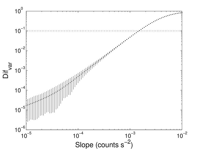
Figure 1: The relative variance difference $\rm{Dif_{var}}$ as a function of the slope of the linear trend derived from simulated light curves. The simulated light curves were produced by the superposition of a standard normal random series and a straight line with a certain slope. $\rm{Dif_{var}}$ is the relative difference between the variance before and after removing the linear trend. Each point and its error bar is calculated from 100 simulated light curves.

The definition of variation power assumes that the time series fluctuates about a mean count rate, without long-term trends. In our study we calculated mean variance and power spectra from segments with a length of 800 seconds, hence the test for the presence of a trend was performed for each segment. We centered and scaled the segment light curve by subtracting the mean and dividing by the standard deviation of the corresponding segment. Then we fitted the light curve with a linear model. For the observations 10238b and 10512 studied here, we found the best-fitting slope is of the order of $10^{-4}$ counts s^-2. The relative difference between the variances before and after removing the linear trend is no more than a few percents, which is significantly smaller than the estimated error of variation power. More generally, we did a simple simulation to study the impact of a long-term linear trend to the estimate of the variance. We produced a light curve with a timestep of 1/64 s by adding a standard normal distributed random series and a straight line. We changed the slope of the line and derived the corresponding difference of variances, as shown in Figure 1. In order for the relative difference to be smaller than 10%, the best-fitting slope should not exceed $\sim 10^{-3}$ counts s^-2, or else the corresponding segment should be excluded or detrended before the calculation of variation power.

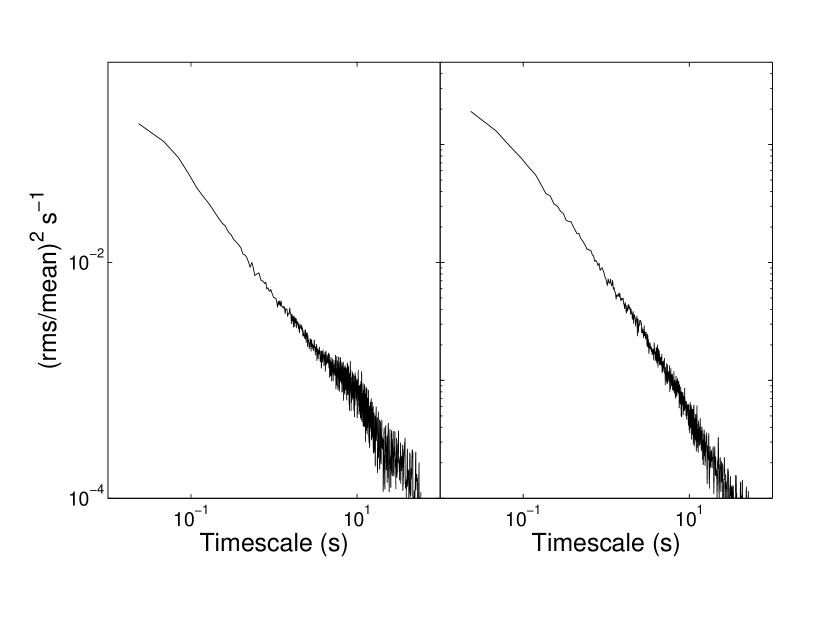
Figure 2: The time domain power spectra of two segments of 10512, respectively belonging to the first and last observation ID.

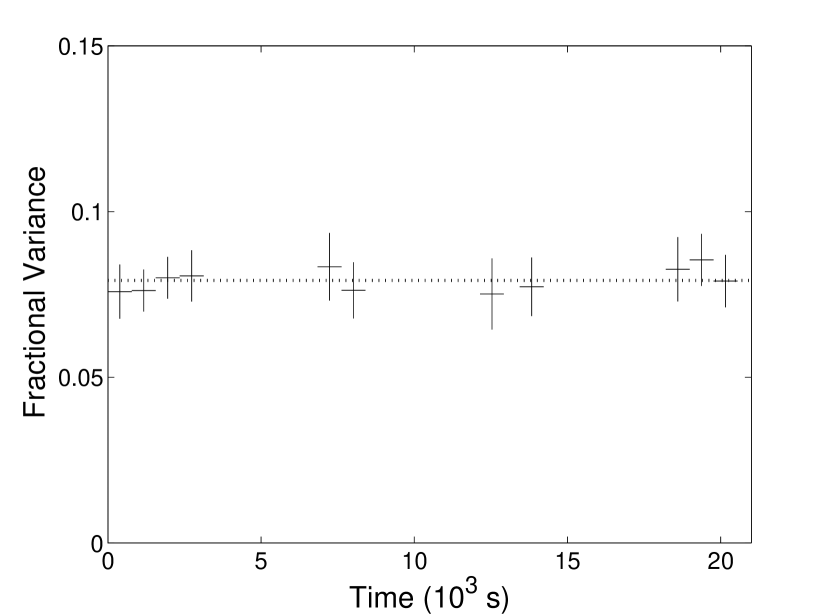
Figure 3: The fractional variances (variance/flux) in different segments of 10238b. The dashed line is the mean value.

The fractional power density on different timescales is obtained from each segment, and then they are averaged to reduce random fluctuations. The average is meaningful only when the intrinsic statistical properties do not depend on time or, in other words, the underlying variability processes are stationary so that the scatters of the power density are simply due to the random fluctuations. The duration of a pointed observation of RXTE is usually only several thousands seconds, but sometimes we have to combine different observations in order to have enough exposure to produce the power density. The time separation between observations could be from hours to days, in which case a test for stationarity is especially necessary. Vaughan et al. (2003) discussed two approaches for testing the stationarity of variability, by comparing PSDs and comparing variances. We performed similar tests to our data. We derived the power spectra of 10512 from 8 observation IDs of P10512 covering 3 days. The time domain power spectra from the first segment and the last segment are shown in Figure 2. No significant difference can be seen. Because it is the fractional power densities from different segments that are averaged, the variance divided by the mean flux (fractional variance) from each segment is compared. Error bars are assigned by measuring the deviation of multiple estimates (Vaughan et al., 2003). We show the example of 10238b in Figure 3, from which the fractional variance is consistent with a constant.

The background shows strong fluctuations on large time scales so that we need to check whether the time domain power spectra are influenced by it. Cyg X-1 is a very bright source and, even for the observation of 10238b in its LH state, the background calibration is only at a level of $\sim 1\%$. We derived the power densities of background on the timescales of tens of seconds without subtracting the poisson noise and found they are one order of magnitude smaller than the source power densities at the same timescale, both for the entire energy range and for a selected energy range. Furthermore, we tried subtracting the background light curve from the source light curve and calculating the time domain power spectrum from the net light curve. We found it to exhibit a difference generally about a few percents with the previous one. The role of background fluctuations is therefore not significant for Cyg X-1.

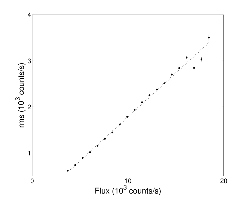
Figure 4: The rms-flux relation of 10512 in the channel region of 0–35, corresponding to 2–13 keV.

On the other hand, when the source in its HS state at high flux, we need to take care of a possible buffer overflow suffered by binned data mode. For the data configuration B_4ms_8A_0_35_H, 8-bit counters are used to form the binned spectrum during each 4 ms binning interval; that is, up to 256 counts can be accumulated per 4 ms without overflowing. The buffer overflow usually occurs in the low energy band, in which it will have a remarkable effect on timing properties such as rms (see e.g., Gleissner et al., 2004). According to the RXTE Technical Appendix, the maximum rate of events that can be supported without overflowing for the binned mode data used here is 256,000 counts s^-1, which is much larger than the mean count rate of $\sim 8,600$ and the maximum count rate of $\sim 42,000$ for 10512. We also derived the rms-flux relation with the method in Gleissner et al. (2004), which exhibits a rather good linear relation (Figure 4). If the data suffered buffer overflow, the rms-flux relation would display an arch-like shape. The conclusion is that our data are not effected by buffer overflow.

After checking the data for the possible systematic biases introduced by the long-term trends, the stationarity, the background fluctuations and buffer overflow, we ascertained the validity of the time domain power spectra. Making use of the the time domain power spectra for each energy channel and background-subtracted energy spectra, we obtained TRS in 10 timescale bins covering 0.02–60 s with approximately equal widths in logarithm axis. The uncertainties of TRS were propagated from the corresponding time domain power spectra and time-averaged energy spectra.

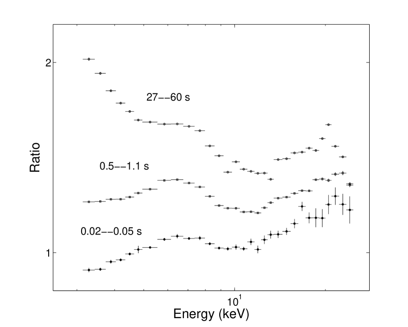
Figure 5: The ratio of TRS for the timescales of 0.05–0.1 s (dots), 0.5–1.1 s (squares) and 27–60 s (circles) of 10238b to a power law model with the photon index of 1.9. They are rescaled for clarity.

The ratios of TRS to a power law model with photon index of 1.9 are shown in Figure 5, which visibly exhibits the distinct characteristics of spectral shapes in different timescale ranges. In the long timescale range (27–60 s), the TRS has a “soft excess” below 4 keV, an broad line around 6–7 keV and a smeared edge above $\sim 7$ keV. In contrast, the TRS in the short timescale range (0.05–0.1 s) lacks of the above features below 10 keV, and exhibits a much more prominent hard component around 20 keV. The shape of the TRS in the medium timescale range (0.5–1.1 s) is between those in the long and short timescale ranges, indicating a continuous evolution of TRS shape with timescale. Therefore it seems that TRS turns softer and has more prominent feature of iron line, as the timescale increases.

TRS were fit in the energy range of 3–13 keV with XSPEC v12.3.1. We selected a simple model consisting of a power law and a Gaussian line to represent the iron fluorescent line. The low energy absorption was obtained from the HEASARC website (http://heasarc.gsfc.nasa.gov/cgi-bin/Tools/w3nh/w3nh.pl) and fixed at $N_{\rm{H}}=7\times 10^{21}$ cm^-2. Such a spectral model is obviously oversimplified, and the reasons we chose it are: 1) the TRS of 10512 (produced from B_4ms_8A_0_35_H configuration) has only 7 energy channels in 3–13 keV band, restricting the use of more sophisticated models; 2) the aim of the spectral fit is to quantitatively measure the observed spectral features, instead of determining the precise best-fitting model and reveal the true underlying physics; 3) this is the model used in the previous FRS analysis for the same data (Revnivtsev et al., 1999; Gilfanov et al., 2000) and the spectral parameters can be directly compared with those of FRS. The energy of iron fluorescent line was fixed at 6.4 keV, and its width was fixed at 0.6 and 0.8 keV for 10238b and 10512 respectively, which are the best-fitting values from the corresponding Standard 2 energy spectra. A uniform systematic error of $0.8\%$ was added to all the channels when fitting TRS. The free parameters include the normalization and the photon index of the power law, and the normalization of the Gaussian line.

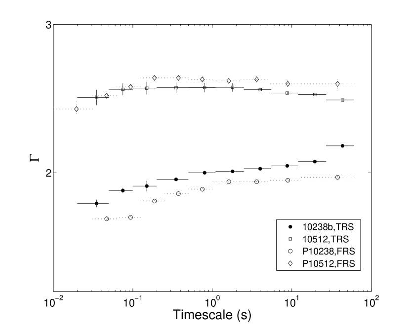
Figure 6: The dependence of the power law photon index ($\Gamma$) on timescale for 10238b (dots, solid line) and 10512 (squares, solid line). The results from FRS (Gilfanov et al., 2000) are also plotted for the observation P10238 (circles, dotted line) and P10512 (diamonds, dotted line).

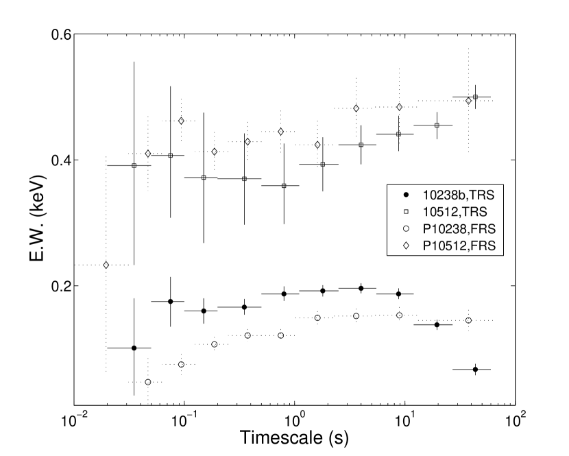
Figure 7: The dependence of the equivalent width (E.W.) of the iron fluorescent line on the timescale for 10238b (dots, solid line) and the 10512 state (squares, solid line). The results from FRS (Gilfanov et al., 2000) are also plotted for the observation P10238 (circles, dotted line) and P10512 (diamonds, dotted line).

We are interested in the best-fitting power law photon index ($\Gamma$) and the equivalent width (E.W.) of iron fluorescent line, as listed in Table 2. The dependence of the above two parameters on the timescale are plotted in Figure 6 and Figure 7 respectively. The relation of $\Gamma$ and timescale exhibits a positive correlation for 10238b. For 10512 it appears that as the timescale increases, $\Gamma$ increases first, then keeps stable and finally decreases. However, the relative amplitude of variation of $\Gamma$ is smaller than 10238b. The E.W. of 10238b increases with increasing timescale below $\sim$0.1 s, and stays almost constant in the range 0.1 s–10 s, then decreases above $\sim$10 s. For the E.W. of 10512, the relative variation amplitudes are smaller and the uncertainties are larger. The most prominent difference in comparison with 10238b is that the E.W. does not show the drop at short timescales, but exhibits a rising trend at long timescales (several tens of seconds). We also took the data of $\Gamma$ and E.W. from Gilfanov et al. (2000), translated frequency into timescale and plotted the result in the same figures. The similarities are clear. See the discussion section for a specific comparison between TRS and FRS for the observations around the 1996 state transition.

3.2 Application to Other Observations of Cyg X-1

We have applied TRS to the data of P10238 and P10512, and compared it with the FRS results from the same data. We discovered that the two methods do reveal the similar phenomena, which supports the feasibility of the novel technique of TRS. RXTE has been operated for more than a decade and a large amount of observational data have been accumulated. We tried to extend the application of TRS to a larger data set.

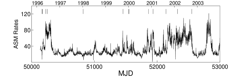
Figure 8: The ASM light curve covering the observations in our study. The small, solid vertical lines in the top indicate the times of observations listed in Table 1.

To take full advantage of TRS, we require the data with high time resolution (higher than 1/64 s), good energy resolution (no less than 8 energy bins covering the channel range 0–35), and enough exposure time. We searched the RXTE archive for suitable observations of Cyg X-1 and found the Generic Binned configurations B_16ms_64M_0_249, B_16ms_46M_0_49_H and B_4ms_8A_0_35_H fulfil our demands. The first two configurations have only one proposal, which are P10238 and P30157 respectively. The proposals containing the configuration B_4ms_8A_0_35_H are P10214, P10412, P10512, P40101, P40102, P50109, P60089, P70104. Another very common configuration B_2ms_8B_0_35_Q has only two energy bins between $\sim$ 5–8 keV and is not a best choice for detecting on iron line. We have produced 11 TRS with the data from the above proposals in addition to 10238b and 10512 studied in the last section. Table 1 displays the observation IDs used, as well as the observation dates and exposure times for each TRS. Figure 8 marks their locations on the overall ASM light curve. The data analysis followed the same procedures outlined before.

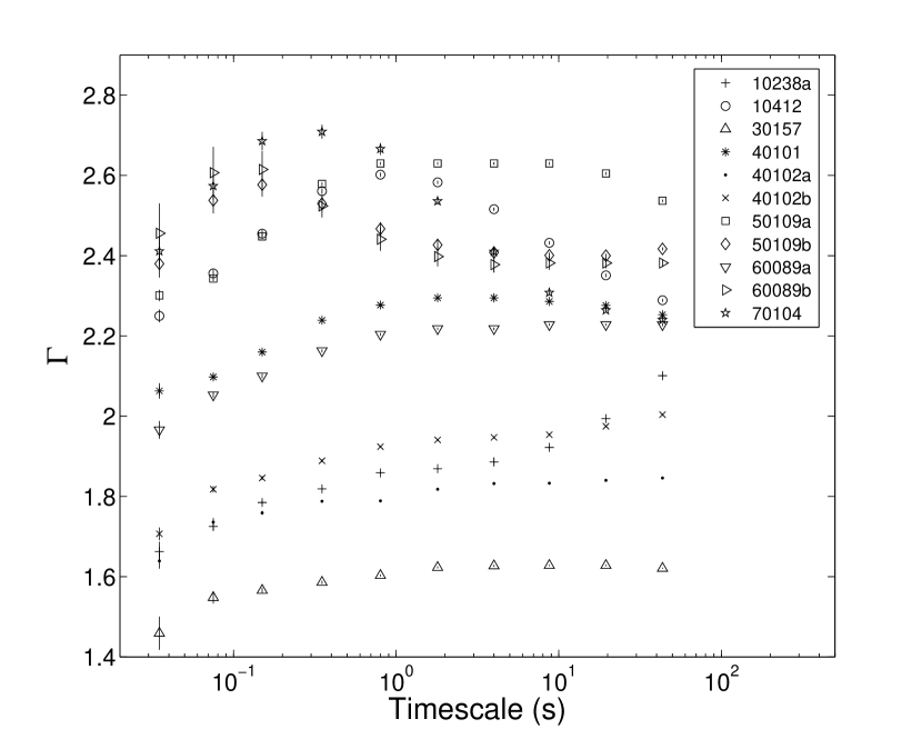
Figure 9: The best-fitting power law photon index ($\Gamma$) as a function of timescale.

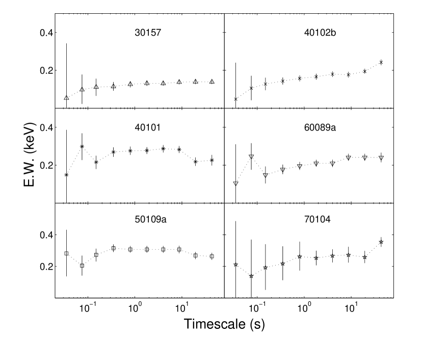
Figure 10: The equivalent width (E.W.) of the iron fluorescent line as a function of timescale for six of the observations.

We plotted the power law photon indices for different timescales in Figure 9. The behaviors of different observations corresponding to different average $\Gamma$ are different: in the lower part of Figure 9 (or quantitatively for the observations with maximum $\Gamma<\sim 2.2$) $\Gamma$ increases with timescale until $\sim 1$ s, and then remains almost constant (except 10238a which shows a strong rise at timescales $>\sim 10$ s, similar to 10238b); for the observations with maximum $\Gamma>\sim 2.2$, $\Gamma$ first rises with timescale, then drops down at larger timescales. This evolution of $\Gamma$ with timescale is similar to 10512, but the latter is much smoother. The equivalent widths of iron line on different timescales were also studied and the representive cases are plotted in Figure 10. The shape of the relation between E.W. and timescale can be roughly divided into three types, each corresponding to one row of Figure 10. The observations with the E.W. evolution shown in the top row of Figure 10 locate in the lower part of Figure 9. 40101 and 60089a, which have a similar evolution of E.W. (the middle row in Figure 10), are also very close to each other in the middle section of Figure 9. The observations in the upper part of Figure 9, characterized by the drop of $\Gamma$ at large timescale, corresponds to the bottom row of Figure 10. Taking the previous observations, 10238b and 10512 into consideration, we found 10512 obviously consistent with the performance of the last type of observations. However, 10238b is more complex and will be discussed below.

4 DISCUSSION

4.1 Comparison with FRS

Comparing the results of TRS with FRS for Cyg X-1 (Revnivtsev et al., 1999; Gilfanov et al., 2000), we found that: 1) the shapes of the three TRS divided by a power law in Figure 5 are similar to FRS in the corresponding frequency ranges (see Figure 1 in Revnivtsev et al. 1999 for the ratios of FRS to a power law, in the frequency ranges of 0.03–0.05 Hz, 4.5–6.8 Hz and 23–32 Hz); 2) the dependencies of the power law photon index on timescale are consistent for TRS and FRS, $\Gamma$ increases with the timescale for both states when the timescale is below $\sim 0.1$ s, and exhibits a decreasing trend at timescales larger than $\sim 10$ s for the HS state (P10512); 3) the relation of equivalent width of iron fluorescent line versus timescale obtained from TRS, however, is inconsistent with that of FRS (see Figure 3 in Gilfanov et al. 2000). In the HS state (P10512), the E.W. drops dramatically at a timescale of 20–30 ms for FRS, which is absent in the case of TRS. However, this is probably because TRS does not extend to timescales as low as FRS (see Figure 7) and therefore misses the drop. In the LH state (P10238), the E.W. obtained from both FRS and TRS drop at timescales shorter than 0.5–1 s. But at longer timescales, between 10–100 s, the E.W. decreases significantly only for TRS.

The similar phenomena revealed by TRS and FRS prove that TRS is another useful tool capable of studying jointly the spectral and timing properties of X-ray source. It provides the amplitude of variability in a certain timescale range as a function of energy. The important practical property of TRS is that they receive the contributions only from the spectral components that are variable on the timescale sampled. Therefore by computing TRS we can investigate whether different spectral components in the average energy spectrum of the sources (e.g. disk blackbody, power law, iron fluorescent line) are variable in a given timescale range. Furthermore, the comparison of TRS with the average energy spectrum could be employed to study the relative variability amplitudes of various spectral components at a given timescale.

4.2 The Variation of 10238b at Large Timescales

The most remarkable difference between TRS and FRS is that for the former, the E.W. of 10238b decreases at long timescales ($>$10 s). What’s more, the behaviors of 10238b at long timescales are in fact unusual compared to other observations. Except 10238a, which belongs to the same proposal number, we can not find others that display the drop of E.W. and the rise of $\Gamma$ at timescales of tens of seconds.

The most straightforward explanation for the variation behavior of the iron line in the TRS is in terms of a finite light-crossing time to the distance of the reflector (Revnivtsev et al., 1999; Gilfanov et al., 2000). The high frequency at which the E.W. drops is considered to be the inverse of the light crossing time between the primary source (assumed as an isotropic point source above a flat disk in Gilfanov et al. 2000, and very likely the hard X-ray-emitting corona) and the reflector (or more specifically, the inner radius of the disk that can process the X-ray continuum radiation and produce the iron line). With this characteristic frequency, Gilfanov et al. (2000) estimated the inner radius of the disk to be $R_{\rm{in}}\sim 100~{}R_{\rm{g}}$ in the LH state and $R_{\rm{in}}\leq 10~{}R_{\rm{g}}$ in the HS state. In this context, the decreases of E.W. at both small and large timescales may reflect the finite spatial extend of the reflector, for example, the inner and outer radius of the reprocessing disk. The timescales at which the equivalent widths drop by a factor of $\geq 2$ are about 0.04 s and 40 s, corresponding to a distance of $1\times 10^{9}$ cm and $1\times 10^{12}$ cm respectively. For a 10 $M_{\odot}$ black hole, it might indicate an inner and outer disk radius of $300~{}R_{\rm{g}}$ and $3\times 10^{5}~{}R_{\rm{g}}$ respectively. The inner radius is consistent with the transition radius of $\geq 100~{}R_{\rm{g}}$ in the LH state predicted by Advection-Dominated Accretion Flow (ADAF) model (e.g., Esin et al., 1998). With a compact star mass of 10 $M_{\odot}$, a mass ratio of 3 (Gies et al., 2003) and an orbital period of 5.6 d (Gies & Bolton, 1982), we estimated the tidal radius of accretion disk as $3\times 10^{5}~{}R_{\rm{g}}$, also consistent with the outer disk radius obtained from the dependence of E.W. on the timescale.

The finite geometry extent of the reprocessing matter is not an unique way to interpret the variation behaviors of E.W. on different timescales. Actually it cannot explain why the decrease of the E.W. at large timescales is not present in other observations, considering that Cyg X-1 is a persistent source and therefore the size of its accretion disk should not have a violent change. The drop of E.W. at large timescales in 10238b is likely to be caused by other reasons. Taking notice of the poor goodness of fit for TRS at the timescale of 27–60 s, as well as the soft spectral shape for the same timescale in Figure 5, we believe that the simple model used before is not proper here any more and an additional soft disk component should be present. The TRS at 27–60 s was fitted again with a model consisting of a disk blackbody, a power law and a Gaussian line. The reduced $\chi^{2}$ improved from $331.79/16$ to $27.15/14$, while $\Gamma$ decreased from 2.18 to 2.09 and the E.W. increased from 0.067 keV to 0.138 keV. It means that after including the disk component in the model, the striking changes of $\Gamma$ and E.W. at large timescales disappear. Both parameters stay almost constant at least up to tens of seconds. Therefore the strange variation of 10238b is probably an artifact due to the presence of a strong soft component. We suggest that in this case the disk component is not variable on timescales shorter than $\sim$10 s, while $\Gamma$ and E.W. keep constant at the timescale larger than $\sim$10 s. Although the variability in the disk component was absent in the previous FRS study of Cyg X-1, it was indeed found in other sources. In the neutron star LMXB GX 340+0, the power density spectrum of the disk appears to follow a power law $P_{\rm{disk}}(f)\propto f^{-1}$, contributing to the overall variability at low frequency ($<\sim 0.5$ Hz) only (Gilfanov et al., 2003). The variation of the disk blackbody component is related to the viscous instability of the accretion disk and the variation of the power law spectral component is related to the thermal instability (Miyamoto et al., 1994). The absence of rapid variability for disk component is consistent with the amplitude of the viscous timescale (e.g., Reig et al., 2006).

10238a shows similar variations with 10238b at large timescales and can also be modified by introducing a soft disk component. The other observations with a much lower energy resolution and degrees of freedom can not be fitted with a model with an additional disk component. However $\chi^{2}$ usually increases at the largest timescale, which possibly implies the need for a reconsideration of the applied model. After this modification to the variation at large timescales, the $\Gamma$ and E.W. of 10238a and 10238b behave alike other observations.

4.3 The Classification of Observations

There exist good correspondences between the relations of $\Gamma$ with timescale and the relation of E.W. with timescale. Based on the correspondences, we are able to classify the observations analyzed in this paper into three types.

The first type includes observations 10238a, 10238b, 30157, 40102a, 40102b. The characteristics of this type of observations can be summarized as (for 10238a and 10238b, the modifications to the variations at large timescales discussed above have been considered): 1) $\Gamma$ has a positive correlation with timescale below $\sim 1$ s, and stays almost constant above $\sim 1$ s, with the maximum value of $<2.1$; 2) E.W. decreases when timescale is smaller than $\sim 0.1$ s, and keeps flat or evolves smoothly at larger timescale. This type can be readily connected with the LH state because of the low values of $\Gamma$ (e.g. McClintock & Remillard, 2006). Indeed all the observations were operated when Cyg X-1 in its LH state. 10238a and 10238b were before the state transition occurred at 1996 May 10 (Cui et al., 1997; Belloni et al., 1996), and 30157 was at the long “quiet” LH state starting from the end of the HS state in 1996 until 1998 July. Then Cyg X-1 entered a episode with several major flares. 40102a and 40102b were in the interval of these flares or “failed state transitions” (e.g. Pottschmidt et al., 2003).

The second type contains observations 10412, 10512, 50109a, 50109b, 60089b and 70104. Here: 1) $\Gamma$ increases with timescale below $\sim 0.5$ s, but shows a prominent decrease at timescales above $\sim 1$ s. The maximum values of $\Gamma$ is larger than 2.4; 2) the E.W. does not decrease significantly at the timescale of $\sim 0.1$ s, instead it may have some increasing trend at short timescales. This type of observations should be linked with the HS state according to the large value of $\Gamma$. As to their observation dates, 10412 and 10512 are observed in the HS state of 1996 (according to the detailed phase division in Cui et al. 1997, 10412 is located at the LH to HS transition phase, but the flux is at the same level as the following HS state). 50109a and 50109b are observed during a period of intense flaring, which started in 2000 October and lasted until 2001 March. Both the peak flux and the minimum hardness ratio reached by the flares are nearly identical to those of the 1996 state transition, and the source did enter a period that resembles a sustained HS state during the last outburst (Cui et al., 2002). 60089b and 70104 are observed during the long 2001/2002 HS state staring from 2001 November (e.g. Zdziarski et al., 2002; Wilms et al., 2006).

The third type includes observations 40101 and 60089a and is described as: 1) the behavior of $\Gamma$ is similar to the first type, but with a maximum value around 2.2, and sometimes exhibits a slight decreasing trend at large timescales, like the second type; 2) E.W. shows a complex behavior at short timescales, increases at $\sim 1$ s but decreases dramatically at smaller timescales. This type seems like between the first two types, and therefore could be related with the intermediate state between the LH state and the HS state. 40101 was observed on 1999 October, when Cyg X-1 was experiencing a major flare (Pottschmidt et al., 2003). 60089a is at the initial stage of 2001/2002 state transition. It is worth to notice that 10238b, although classified into the first type, indeed shows some similar features with this type, such as the values of $\Gamma$ and the E.W. at short timescales. 10238b was observed during a minor flare before the major HS state of 1996, and it is not surprising to see the similarities because it is not as “low” as the other observations in the first type. So that it appears that the three types of evolution with timescale have tight connections with the spectral states, and the translations from one to another are smooth.

4.4 Physical Interpretation

As discussed in the previous section, there exist good correspondences between the evolutions of $\Gamma$ and E.W. with timescale, and furthermore they can be connected with the conventional spectral states of Cyg X-1. The interpretation for this is not very clear, and up to now most models involving the X-ray production mechanism in the accretion process do not consider such constraints imposed by timescale (frequency) resolved spectral analysis.

The dependence of E.W. on timescale seems in favor of the finite geometry size of the reflector as mentioned above, if we focus on the short timescales. In this picture, the drop of E.W. at timescales $<\sim 0.1$ s in the LH state reflects the finite light-crossing time between the primary source and the reflector. However in the HS state E.W. keeps flat down to timescales $<\sim 0.1$ s, which indicates a much smaller distance between primary source and reflector. This can be explained by the different inner radius of accretion disk for the two spectral states, just as stated in Gilfanov et al. (2000).

The spectral slope generally decreases with decreasing timescale or increasing frequency, which has been proved prevalent in the FRS study on black-hole binaries, neutron star LMXBs and AGNs. But in our study it is only true for the timescales shorter than $\sim 0.1$ s to $\sim 1$ s depending on the spectral states. Papadakis et al. (2007) discussed two kinds of models that can qualitatively explain the fact based on FRS that the spectral shape becomes softer at larger timescales. One is the phenomenological model attributes the variable emission to multiple active regions moving towards the central compact object (Życki, 2003). This model assumes that the Comptonized spectrum evolves from softer to harder during the flare evolution towards the center with diminishing supply of seed photons. The other explanation is in the context of ADAF, where the Comptonization parameter increases with decreasing radius. A variation at short timescale originates at small radius with large Comptonization parameter, leading to a hard spectrum. But Życki (2002) predicted an opposite trend to FRS with the model of magnetic flare radially distributed above an accretion disk with hot ionized skin.

4.5 Application in Weak Sources

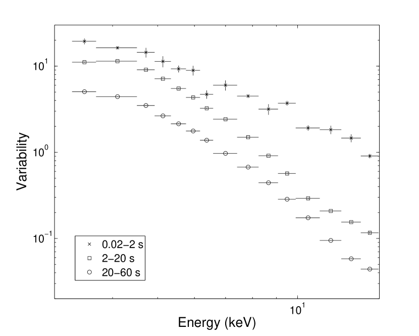
Figure 11: TRS of 4U 1543-47 in three timescale ranges. They are rescaled for clarity.

Cyg X-1 is a perfect target for timing studies because of the large amount of data with different kinds of configurations, its large flux, and its relatively persistent properties compared with transient sources. When the method is applied to some weak sources, there is one additional issue that should be considered. In a faint source, when power is small, the variability due to the source is small compared to the variance due to noise, so that subtracting the expected poisson noise level can sometimes lead to negative variances due to the fluctuation of the true noise level. This problem is also met in the study of FRS (e.g. Papadakis et al., 2005, 2007). The solution is to sacrifice the frequency (timescale) resolution or energy resolution to increase the statistical significance. Broad frequency ranges have to be considered so as to get positive value after accumulating the power densities in each band, therefore FRS is usually derived in only two or three frequency bands (see, e.g. Papadakis et al., 2005; Reig et al., 2006; Papadakis et al., 2007; Shrader et al., 2007; Arévalo et al., 2008). We show an example of TRS in 4U 1534-47 (observation ID 70133-01-04-00) in Figure 11, also studied with FRS in Reig et al. (2006).

In conclusion, TRS is a novel spectral-timing joint analysis technique, which follows FRS but is based on the time domain power spectrum. The aims of both TRS and FRS are to determine the characteristic timescale of the physical process, to probe the origin of the variability, and to reveal the link between physical mechanism and geometry arrangement around compact object. Our work is but a first step. We believe that the application of TRS to more samples, the study of TRS with higher-quality data, the specific comparison between TRS and FRS, and the development of theoretical models will offer a clearer picture and further insight on these issues.

Table 1: The list of RXTE observations used for the analysis.

Abbreviation	Obs. ID	Start Time	Exposure (s)	Configuration
10238a	10238-01-08-00	1996-03-26 10:11	23339	B_16ms_64M_0_249
10238b	10238-01-05-000	1996-03-30 19:47	13381	B_16ms_64M_0_249
10412	10412-01-01-00	1996-05-23 14:20	7791	B_4ms_8A_0_35_H
	10512-01-07-00	1996-06-16 00:01	808
	10512-01-07-02	1996-06-16 04:49	1287
	10512-01-08-01	1996-06-17 01:38	686
10512	10512-01-08-02	1996-06-17 04:50	1286	B_4ms_8A_0_35_H
	10512-01-08-00	1996-06-17 08:02	2126
	10512-01-09-02	1996-06-18 03:15	864
	10512-01-09-00	1996-06-18 06:28	1644
	10512-01-09-01	1996-06-18 09:40	2424
30157	30157-01-05-00	1998-01-08 04:37	4045	B_16ms_46M_0_49_H
	30157-01-06-00	1998-01-15 22:55	4364
40101	40101-01-08-00	1999-10-05 07:14	3587	B_4ms_8A_0_35_H
	40101-01-09-00	1999-10-05 18:33	2744
40102a	40102-01-02-00	2000-01-05 00:39	16386	B_4ms_8A_0_35_H
40102b	40102-01-01-16	2000-01-08 11:48	8786	B_4ms_8A_0_35_H
50109a	50109-03-10-00	2000-11-14 06:10	9781	B_4ms_8A_0_35_H
	50109-01-06-00	2001-01-26 00:00	1557
50109b	50109-01-06-01	2001-01-26 21:39	3145	B_4ms_8A_0_35_H
	50109-01-06-02	2001-01-27 20:11	1710
60089a	60089-01-02-00	2001-08-20 07:25	6084	B_4ms_8A_0_35_H
60089b	60089-03-07-00	2002-02-19 01:08	8033	B_4ms_8A_0_35_H
	60089-03-08-00	2002-02-19 06:08	2254
	70104-01-03-00	2002-10-03 18:56	3561
70104	70104-01-04-00	2002-10-04 18:36	2427	B_4ms_8A_0_35_H
	70104-01-04-01	2002-10-05 17:23	2950

Table 2: Best-fitting parameters of 10238b and 10512.

	LH state (10238b)				HS state (10512)
Timescale(s)	$\Gamma$	E.W.(keV)	$\chi^{2}$		$\Gamma$	E.W.(keV)	$\chi^{2}$
0.02-0.05	1.794$\pm$0.025	0.101(0.026-0.180)	9.39		2.508$\pm$0.051	0.391(0.233-0.556)	1.87
0.05-0.1	1.881$\pm$0.018	0.175(0.125-0.214)	21.14		2.563$\pm$0.040	0.407(0.308-0.517)	1.44
0.1-0.2	1.911$\pm$0.036	0.160(0.140-0.180)	30.30		2.571$\pm$0.043	0.372(0.268-0.475)	4.33
0.2-0.5	1.956$\pm$0.009	0.166(0.154-0.179)	23.57		2.574$\pm$0.034	0.370(0.297-0.442)	2.24
0.5-1.1	2.001$\pm$0.008	0.187(0.176-0.199)	27.44		2.575$\pm$0.031	0.359(0.298-0.426)	2.31
1.1-2.5	2.010$\pm$0.008	0.192(0.183-0.201)	23.31		2.576$\pm$0.029	0.393(0.350-0.436)	5.78
2.5-5.5	2.028$\pm$0.008	0.196(0.188-0.204)	20.02		2.561$\pm$0.006	0.424(0.393-0.455)	5.75
5.5-12	2.047$\pm$0.008	0.187(0.179-0.196)	22.51		2.538$\pm$0.005	0.441(0.414-0.470)	13.58
12-27	2.076$\pm$0.011	0.138(0.130-0.146)	58.17		2.528$\pm$0.004	0.455(0.433-0.476)	17.54
27-60	2.182$\pm$0.002	0.067(0.058-0.076)	331.79		2.491$\pm$0.003	0.500(0.481-0.519)	54.49

Note. — ‘$\Gamma$’–the power law photon index and its uncertainty corresponding to 90% confidence interval; ‘E.W.’–the equivalent width of the iron fluorescent line, with its 90% confidence interval indicated in the brackets. The degrees of freedom are 16 and 4 for 10238b and 10512 respectively.

References

- Arévalo et al. (2008) Arévalo, P., McHardy, I. M., Markowitz, A., Papadakis, I. E., Turner, T. J., Miller, L., & Reeves, J. 2008, MNRAS, 387, 279
- Belloni et al. (1996) Belloni, T., Mendez, M., van der Klis, M., Hasinger, G., Lewin, W. H. G., & van Paradijs, J. 1996, ApJ, 472, L107
- Cui et al. (1997) Cui, W., Zhang, S. N., Focke, W., & Swank, J. H. 1997, ApJ, 484, 383
- Cui et al. (2002) Cui, W., Feng, Y.-X., & Ertmer, M. 2002, ApJ, 564, L77
- Esin et al. (1998) Esin, A. A., Narayan, R., Cui, W., Grove, J. E., & Zhang, S.-N. 1998, ApJ, 505, 854
- Gies et al. (2003) Gies, D. R., et al. 2003, ApJ, 583, 424
- Gies & Bolton (1982) Gies, D. R., & Bolton, C. T. 1982, ApJ, 260, 240
- Gilfanov et al. (2000) Gilfanov, M., Churazov, E., & Revnivtsev, M. 2000, MNRAS, 316, 923
- Gilfanov et al. (2003) Gilfanov, M., Revnivtsev, M., & Molkov, S. 2003, A&A, 410, 217
- Gleissner et al. (2004) Gleissner, T., et al. 2004, A&A, 425, 1061
- Li (2001) Li, T. P. 2001, Chin. J. Astron. Astrophys., 1, 313
- Li & Muraki (2002) Li, T. P., & Muraki, Y. 2002, ApJ, 578, 374
- Markoff et al. (2005) Markoff, S., Nowak, M. A., & Wilms, J. 2005, ApJ, 635, 1203
- McClintock & Remillard (2006) McClintock, J. E., & Remillard, R. A. 2006, Compact stellar X-ray sources, 157
- Miyamoto et al. (1994) Miyamoto, S., Kitamoto, S., Iga, S., Hayashida, K., & Terada, K. 1994, ApJ, 435, 398
- Papadakis et al. (2005) Papadakis, I. E., Kazanas, D., & Akylas, A. 2005, ApJ, 631, 727
- Papadakis et al. (2007) Papadakis, I. E., Ioannou, Z., & Kazanas, D. 2007, ApJ, 661, 38
- Pottschmidt et al. (2003) Pottschmidt, K., et al. 2003, A&A, 407, 1039
- Reig et al. (2006) Reig, P., Papadakis, I. E., Shrader, C. R., & Kazanas, D. 2006, ApJ, 644, 424
- Revnivtsev et al. (1999) Revnivtsev, M., Gilfanov, M., & Churazov, E. 1999, A&A, 347, L23
- Revnivtsev et al. (2001) Revnivtsev, M., Gilfanov, M., & Churazov, E. 2001, A&A, 380, 520
- Revnivtsev & Gilfanov (2006) Revnivtsev, M. G., & Gilfanov, M. R. 2006, A&A, 453, 253
- Shrader et al. (2007) Shrader, C. R., Reig, P., & Kazanas, D. 2007, ApJ, 667, 1063
- Tomsick et al. (2008) Tomsick, J. A., et al. 2008, ApJ, 680, 593
- Vaughan et al. (2003) Vaughan, S., Edelson, R., Warwick, R. S., & Uttley, P. 2003, MNRAS, 345, 1271
- Wilms et al. (2006) Wilms, J., Nowak, M. A., Pottschmidt, K., Pooley, G. G., & Fritz, S. 2006, A&A, 447, 245
- Zdziarski et al. (2002) Zdziarski, A. A., Poutanen, J., Paciesas, W. S., & Wen, L. 2002, ApJ, 578, 357
- Życki (2002) Życki, P. T. 2002, MNRAS, 333, 800
- Życki (2003) Życki, P. T. 2003, MNRAS, 340, 639