Tidal dissipation in rotating fluid bodies: a simplified model

Abstract

We study the tidal forcing, propagation and dissipation of linear inertial waves in a rotating fluid body. The intentionally simplified model involves a perfectly rigid core surrounded by a deep ocean consisting of a homogeneous incompressible fluid. Centrifugal effects are neglected, but the Coriolis force is considered in full, and dissipation occurs through viscous or frictional forces. The dissipation rate exhibits a complicated dependence on the tidal frequency and generally increases with the size of the core. In certain intervals of frequency, efficient dissipation is found to occur even for very small values of the coefficient of viscosity or friction. We discuss the results with reference to wave attractors, critical latitudes and other features of the propagation of inertial waves within the fluid, and comment on their relevance for tidal dissipation in planets and stars.

1 Introduction

Tidal interactions determine the fate of short-period extrasolar planets. They affect their spin and orbital parameters, and in extreme cases may lead to the destruction of planets as a result of orbital decay or intense tidal heating. Tidal evolution is also important in close binary stars and in the satellite systems of the planets of the solar system.

The efficiency of these processes is often parametrized by the tidal quality factor $Q$, which is a dimensionless inverse measure of the dissipative properties of the body considered as a forced oscillator (e.g. Goldreich & Soter, 1966). The tidal $Q$ of fluid bodies such as stars and giant planets is difficult to calculate from first principles, even in linear theory. The tidal disturbance generally consists of two parts. One (the ‘equilibrium tide’) is a quasi-hydrostatic bulge that is carried around the body by a smooth velocity field, while the other (the ‘dynamical tide’) consists of internal waves that are excited by the low-frequency tidal forcing and may have a short wavelength. Dissipation of the equilibrium tide can occur through its interaction with turbulent convection, but the damping rate is uncertain, especially when the tidal period is short compared to the convective timescale (Zahn, 1966b, 1977; Goldreich & Keeley, 1977; Goldreich & Nicholson, 1977; Goodman & Oh, 1997; Penev et al., 2007). This approach has perhaps been most successful in application to the circularization of binaries containing a giant star (Verbunt & Phinney, 1995), in which case the tidal period exceeds the convective timescale. To study dynamical tides one should consider the excitation, propagation and dissipation of low-frequency internal waves in rotating, stratified fluids. Calculations have been made for a variety of objects, using different simplifications and approximations, by Zahn (1970, 1975, 1977), Savonije & Papaloizou (1983, 1984), Savonije, Papaloizou & Alberts (1995), Savonije & Papaloizou (1997), Papaloizou & Savonije (1997), Lubow, Tout & Livio (1997), Terquem et al. (1998), Goodman & Dickson (1998), Witte & Savonije (1999), Savonije & Witte (2002), Ogilvie & Lin (2004, 2007), Wu (2005a, b), Papaloizou & Ivanov (2005) and Ivanov & Papaloizou (2007). This approach has perhaps been most successful for early-type stars, in which gravity (or inertia-gravity) waves are excited near the base of the radiative envelope and propagate outwards until they are dissipated by radiative damping; in this case estimates can be made rather simply for the dissipation rate (or tidal torque) that are independent of the details of the wave damping mechanism (Goldreich & Nicholson, 1989).

In recent work on dynamical tides in rotating giant planets and stars (Ogilvie & Lin, 2004, 2007) we have emphasized the role of inertial waves in convective regions, which are nearly adiabatically stratified and do not support gravity waves (see also Wu, 2005a, b; Papaloizou & Ivanov, 2005; Ivanov & Papaloizou, 2007). Inertial waves (Greenspan, 1968) propagate in a uniformly rotating fluid at frequencies $\omega$ smaller in magnitude than twice the spin frequency $\Omega$, as seen in a frame rotating with the fluid. The group velocity of an inertial wave is proportional to its wavelength and is inclined at an angle $\lambda=\arcsin|\omega/2\Omega|$ to the rotation axis. The behaviour of rays propagating within a spherical annulus (a thick spherical shell) is very complicated and sensitive to the value of $\lambda$ (Rieutord, Georgeot & Valdettaro, 2001). It generally involves the focusing of rays towards limit cycles known as wave attractors. Another important feature is the existence of a critical latitude (equal to $\lambda$) at which the rays are tangent to the core and a singularity is introduced into solutions of the inviscid wave equations. Numerical investigations indicate that the tidally forced disturbances in this frequency range are concentrated in narrow beams whose width diminishes as the viscosity $\nu$ is reduced (Ogilvie & Lin, 2004). In certain intervals of $\omega/\Omega$, a dissipation rate that appears to be asymptotically independent of $\nu$ may be achieved. However, the dissipation rate varies in a complicated way with the tidal frequency; presumably this occurs because of the sensitivity of the ray propagation to the value of $\lambda$, and depends on the waves being reflected from the inner and outer boundaries.

In an attempt to understand aspects of this behaviour, we have investigated a variety of reduced models. Using a prototypical partial differential equation for internal waves (Ogilvie, 2005), we studied the response to periodic forcing in a two-dimensional domain in which the rays are focused towards a single wave attractor, as occurs in the experiments of Maas et al. (1997) and Manders & Maas (2003). We constructed an asymptotic analytical solution and showed that a non-zero dissipation rate is achieved in the astrophysically relevant limit of small viscosity (i.e. small Ekman number). This limiting dissipation rate is independent of the magnitude and even of the form of the small-scale damping mechanism for the waves, which is very promising for astrophysical applications. We confirmed the analytical solution in detail using numerical methods.

The method used by Ogilvie (2005) cannot be applied directly to the problem of tidal forcing when the fluid occupies a spherical annulus. One technical complication is that the hyperbolic equation describing the structure of inviscid inertial waves in the meridional plane of a spherical system does not possess Riemann invariants, which makes it difficult to describe the propagation of the solution along the characteristics (which are also the ray paths described above). More importantly, the spherical annulus has a concave inner boundary with a critical latitude singularity. Although such a feature could be introduced into the problem considered by Ogilvie (2005) by choosing a domain of an appropriate shape, separate consideration would have to be given to the waves generated by the singularity.

In the present paper we consider a different idealized model that displays the essential features of inertial waves propagating within a spherical annulus and allows a detailed numerical investigation. It involves a perfectly rigid core surrounded by a deep ocean consisting of a homogeneous incompressible fluid. Centrifugal effects are neglected, but the Coriolis force is considered in full, and dissipation occurs through viscous or frictional forces. Although the assumption of a homogeneous incompressible fluid is made for maximal simplicity, the model may be more or less directly applicable to planets or moons involving a deep ocean. We formulate the problem of tidal forcing in Section 2, introduce a further simplification in Section 3 and present numerical solutions in Section 4. The results are discussed in Section 5 and a conclusion follows in Section 6.

2 The tidal problem

2.1 Basic equations

We consider a simplified model of a planet in uniform rotation with angular velocity ${\mn@boldsymbol{\Omega}}=\Omega\,{\mn@boldsymbol{e}}_{z}$. Let $(r,\theta,\phi)$ be spherical polar coordinates in the rotating frame. A perfectly rigid core occupies the region $0<r<\alpha R$ and is surrounded by a homogeneous incompressible fluid with a free surface at $r=R$. We neglect the centrifugal distortion, which is of second order in $\Omega$. Let the mean density of the system be $\bar{\rho}$ and that of the fluid $\rho=\beta\bar{\rho}$. The surface gravity is then

$$g=\frac{4}{3}\pi G\bar{\rho}R.$$ (1)

We consider the long-term response of the system to a tidal gravitational potential $\mathrm{Re}[\Psi(r,\theta,\phi)\,\mathrm{e}^{-\mathrm{i}\omega t}]$, where $\omega$ is the (real) tidal frequency in the rotating frame. The linearized equations within the fluid are

$$-\mathrm{i}\omega{\mn@boldsymbol{u}}+2{\mn@boldsymbol{\Omega}}\times{\mn@boldsymbol{u}}=-{\mn@boldsymbol{\nabla}}W+{\mn@boldsymbol{f}},$$ (2)

$$W=\frac{p^{\prime}}{\rho}+\Phi^{\prime}+\Psi,$$ (3)

$${\mn@boldsymbol{\nabla}}\cdot{\mn@boldsymbol{u}}=0,$$ (4)

$$\nabla^{2}\Phi^{\prime}=4\pi G\rho^{\prime}=-4\pi G\rho\frac{u_{r}}{\mathrm{i}\omega}\delta(r-R),$$ (5)

where ${\mn@boldsymbol{u}}$, $\rho^{\prime}$, $p^{\prime}$ and $\Phi^{\prime}$ are the Eulerian perturbations of velocity, density, pressure and gravitational potential, assumed to have the same form of time-dependence as the tidal potential, and $\delta$ is the Dirac delta function. We include a dissipative force (per unit mass) ${\mn@boldsymbol{f}}$, in the form of either a Navier–Stokes viscous force

$${\mn@boldsymbol{f}}_{\mathrm{v}}=\nu\nabla^{2}{\mn@boldsymbol{u}},$$ (6)

where $\nu$ is the kinematic viscosity, or a frictional damping force

$${\mn@boldsymbol{f}}_{\mathrm{f}}=-\gamma{\mn@boldsymbol{u}},$$ (7)

where $\gamma$ is the frictional damping coefficient. The latter case is artificial but is mathematically and computationally more convenient. In Ogilvie (2005) we found that the asymptotic dissipation rate in a wave attractor is identical for viscous and frictional forces. We set ${\mn@boldsymbol{f}}={\mn@boldsymbol{f}}_{\mathrm{v}}+{\mn@boldsymbol{f}}_{\mathrm{f}}$ in this section, although in the numerical analysis below we consider each type of dissipative force separately.

The time-averaged energy dissipation rate is

$$D=-\frac{1}{2}\,\mathrm{Re}\int_{V}\rho{\mn@boldsymbol{u}}^{*}\cdot{\mn@boldsymbol{f}}\,\mathrm{d}V=-\frac{1}{2}\,\mathrm{Re}\int_{S}\rho W{\mn@boldsymbol{u}}^{*}\cdot\mathrm{d}{\mn@boldsymbol{S}},$$ (8)

where $S$ is the bounding surface of the volume $V$ occupied by the fluid. The last equality follows from the linearized equations and the divergence theorem. For viscous and frictional damping we have

$$D_{\mathrm{v}}=\int_{V}\rho\nu e_{ij}^{*}e_{ij}\,\mathrm{d}V,$$ (9)

$$D_{\mathrm{f}}=\frac{1}{2}\int_{V}\rho\gamma|{\mn@boldsymbol{u}}|^{2}\,\mathrm{d}V,$$ (10)

where $e_{ij}={\textstyle\frac{1}{2}}(\partial_{i}u_{j}+\partial_{j}u_{i})$ is the rate-of-strain tensor in Cartesian coordinates. In the viscous case, either no-slip or stress-free boundary conditions are required to ensure that there is no viscous flux of energy out of the fluid volume.

2.2 Projection on to spherical harmonics

To solve the linearized equations, we introduce a spheroidal–toroidal decomposition and a projection on to spherical harmonics (Zahn, 1966a). Thus

$$u_{r}=\sum a_{n}(r)Y_{n}^{m}(\theta,\phi),$$ (11)

$$u_{\theta}=r\sum\left[b_{n}(r)\frac{\partial}{\partial\theta}+\frac{c_{n}(r)}{\sin\theta}\frac{\partial}{\partial\phi}\right]Y_{n}^{m}(\theta,\phi),$$ (12)

$$u_{\phi}=r\sum\left[\frac{b_{n}(r)}{\sin\theta}\frac{\partial}{\partial\phi}-c_{n}(r)\frac{\partial}{\partial\theta}\right]Y_{n}^{m}(\theta,\phi),$$ (13)

$$W=\sum W_{n}(r)Y_{n}^{m}(\theta,\phi),$$ (14)

$$\Phi^{\prime}=\sum\Phi^{\prime}_{n}(r)Y_{n}^{m}(\theta,\phi),$$ (15)

where the sums are carried out over integers $n\geq m\geq 0$, and

$$Y_{n}^{m}(\theta,\phi)=\left[\frac{(2n+1)(n-m)!}{4\pi(n+m)!}\right]^{1/2}P_{n}^{m}(\cos\theta)\,\mathrm{e}^{\mathrm{i}m\phi}$$ (16)

is a spherical harmonic, satisfying the orthonormality relation

$$\int_{0}^{2\pi}\!\int_{0}^{\pi}[Y_{n}^{m}(\theta,\phi)]^{*}Y_{n^{\prime}}^{m^{\prime}}(\theta,\phi)\sin\theta\,\mathrm{d}\theta\,\mathrm{d}\phi=\delta_{mm^{\prime}}\,\delta_{nn^{\prime}}.$$ (17)

Bearing in mind the linearity of the problem, we consider a forcing potential in the form of a single solid spherical harmonic,

$$\Psi=\Psi_{\ell}(r)Y_{\ell}^{m}(\theta,\phi),$$ (18)

for some $\ell\geq m$. (Although $\Psi_{\ell}\propto r^{\ell}$, only the value $\Psi_{\ell}(R)$ of the potential at the free surface is significant in the case of an incompressible fluid.) The dominant tidal potentials are the quadrupole components with $\ell=2$, and of these the case $m=2$ is usually the most important. The linearized equations couple together different values of $n$ through the Coriolis force, while different values of $m$ are decoupled.

Projecting the equations on to spherical harmonics, we obtain

$$(-\mathrm{i}\omega+\gamma)a_{n}-2\mathrm{i}m\Omega rb_{n}$$ (19)

$$+2\Omega r[(n-1)q_{n}c_{n-1}-(n+2)q_{n+1}c_{n+1}]$$

$$=-\frac{\mathrm{d}W_{n}}{\mathrm{d}r}-n(n+1)\frac{\nu}{r^{2}}\left[a_{n}-\frac{\mathrm{d}}{\mathrm{d}r}(r^{2}b_{n})\right],$$

$$-\mathrm{i}\omega_{n}r^{2}b_{n}-\frac{2\mathrm{i}m\Omega ra_{n}}{n(n+1)}$$ (20)

$$+2\Omega r^{2}[(n-1)\tilde{q}_{n}c_{n-1}+(n+2)\tilde{q}_{n+1}c_{n+1}]=-W_{n}$$

$$+\nu\left[\frac{2a_{n}}{r}+\frac{1}{r^{2}}\frac{\mathrm{d}}{\mathrm{d}r}\left(r^{4}\frac{\mathrm{d}b_{n}}{\mathrm{d}r}\right)-(n-1)(n+2)b_{n}\right],$$

$$-\mathrm{i}\omega_{n}r^{2}c_{n}+2\Omega r(\tilde{q}_{n}a_{n-1}-\tilde{q}_{n+1}a_{n+1})$$ (21)

$$-2\Omega r^{2}[(n-1)\tilde{q}_{n}b_{n-1}+(n+2)\tilde{q}_{n+1}b_{n+1}]$$

$$=\nu\left[\frac{1}{r^{2}}\frac{\mathrm{d}}{\mathrm{d}r}\left(r^{4}\frac{\mathrm{d}c_{n}}{\mathrm{d}r}\right)-(n-1)(n+2)c_{n}\right],$$

$$\frac{1}{r^{2}}\frac{\mathrm{d}}{\mathrm{d}r}(r^{2}a_{n})-n(n+1)b_{n}=0,$$ (22)

where

$$\omega_{n}=\omega+\frac{2m\Omega}{n(n+1)}+\mathrm{i}\gamma,$$ (23)

$$q_{n}=\left(\frac{n^{2}-m^{2}}{4n^{2}-1}\right)^{1/2},\qquad\tilde{q}_{n}=\frac{q_{n}}{n}.$$ (24)

These equations agree with those of Rieutord & Valdettaro (1997) and Ogilvie & Lin (2004) in the appropriate limits. They are to be solved for integers $n\geq m$, but in practice the system must be truncated.

The potential perturbation satisfies

$$\frac{1}{r^{2}}\frac{\mathrm{d}}{\mathrm{d}r}\left(r^{2}\frac{\mathrm{d}\Phi_{n}^{\prime}}{\mathrm{d}r}\right)-\frac{n(n+1)}{r^{2}}{\Phi_{n}^{\prime}}=-4\pi G\rho\frac{a_{n}}{\mathrm{i}\omega}\delta(r-R),$$ (25)

and the solution that is well behaved as $r\to 0$ and as $r\to\infty$ is

$$\Phi_{n}^{\prime}=\frac{4\pi G\rho R}{2n+1}\frac{a_{n}(R)}{\mathrm{i}\omega}\times\cases{(r/R)^{n},&$0<r<R$,\cr(r/R)^{-(n+1)},&$r>R$.}$$ (26)

2.3 Boundary conditions

Since the inner boundary is impermeable, $a_{n}=0$ at $r=\alpha R$. At the outer boundary, the normal stress at the perturbed free surface vanishes. Thus $-p_{n}^{\prime}-\rho g(a_{n}/\mathrm{i}\omega)+2\rho\nu(\mathrm{d}a_{n}/\mathrm{d}r)=0$, i.e.

$$W_{n}-2\nu\frac{\mathrm{d}a_{n}}{\mathrm{d}r}+\left[1-\left(\frac{3\beta}{2n+1}\right)\right]\frac{g}{\mathrm{i}\omega}a_{n}=\Psi_{\ell}\delta_{n\ell}$$ (27)

at $r=R$. In the limits of low frequency and low viscosity, $\omega^{2}\ll g\ell/R$ and $\nu\ll gR/\omega$, the first two terms are negligible, and this equation amounts to specifying the radial velocity at the surface. Indeed, it amounts to saying that the radial displacement of the surface is equal to the simple equilibrium tide $-\Psi/g$, with a correction (the term involving $\beta$) due to the self-gravity of the fluid.

When viscosity is included, additional boundary conditions are required. We assume that the tangential stresses vanish at the inner and outer boundaries, so

$$\frac{a_{n}}{r^{2}}+\frac{\mathrm{d}b_{n}}{\mathrm{d}r}=\frac{\mathrm{d}c_{n}}{\mathrm{d}r}=0$$ (28)

at $r=\alpha R$ and $r=R$. The inner boundary could alternatively be treated using the no-slip conditions $b_{n}=c_{n}=0$, which would result in a prominent Ekman or oscillatory boundary layer.

2.4 Dissipation

The time-averaged energy equation for this system has the form

$$\frac{\mathrm{d}F}{\mathrm{d}r}=-d_{\mathrm{v}}-d_{\mathrm{f}},$$ (29)

where

$$F=\frac{1}{2}r^{2}\rho\,\mathrm{Re}\sum_{n}a_{n}^{*}\left(W_{n}-2\nu\frac{\mathrm{d}a_{n}}{\mathrm{d}r}\right)$$ (30)

$$-n(n+1)\nu\left[b_{n}^{*}\left(a_{n}+r^{2}\frac{\mathrm{d}b_{n}}{\mathrm{d}r}\right)+r^{2}c_{n}^{*}\frac{\mathrm{d}c_{n}}{\mathrm{d}r}\right]$$

is the radial energy flux and

$$d_{\mathrm{v}}=\frac{1}{2}r^{2}\rho\nu\sum_{n}n(n+1)\left(\left|\frac{a_{n}}{r}+r\frac{\mathrm{d}b_{n}}{\mathrm{d}r}\right|^{2}+\left|r\frac{\mathrm{d}c_{n}}{\mathrm{d}r}\right|^{2}\right)$$ (31)

$$+3\left|\frac{\mathrm{d}a_{n}}{\mathrm{d}r}\right|^{2}+(n-1)n(n+1)(n+2)(|b_{n}|^{2}+|c_{n}|^{2}),$$

$$d_{\mathrm{f}}=\frac{1}{2}r^{2}\rho\gamma\sum_{n}|a_{n}|^{2}+n(n+1)r^{2}(|b_{n}|^{2}+|c_{n}|^{2})$$ (32)

are the viscous and frictional dissipation rates per unit radius. The integrated energy equation, together with the boundary conditions, relates the total dissipation rate to the surface forcing:

$$D = D_{\mathrm{v}}+D_{\mathrm{f}}$$ (33)

$$= \int_{\alpha R}^{R}(d_{\mathrm{v}}+d_{\mathrm{f}})\,\mathrm{d}r$$

$$= -\frac{1}{2}\rho R^{2}\,\mathrm{Re}\left[a_{\ell}(R)^{*}\Psi_{\ell}(R)\right].$$ (34)

2.5 Frictional non-rotating problem

In the absence of rotation the different spherical harmonics are decoupled. When only a frictional force is present, the solution satisfying the inner boundary condition is

$$a_{\ell}=A\left[\left(\frac{r}{R}\right)^{\ell-1}-\alpha^{2\ell+1}\left(\frac{R}{r}\right)^{\ell+2}\right],$$ (35)

$$b_{\ell}=\frac{A}{r}\left[\frac{1}{\ell}\left(\frac{r}{R}\right)^{\ell-1}+\frac{\alpha^{2\ell+1}}{\ell+1}\left(\frac{R}{r}\right)^{\ell+2}\right],$$ (36)

$$W_{\ell}=(\mathrm{i}\omega-\gamma)Ar\left[\frac{1}{\ell}\left(\frac{r}{R}\right)^{\ell-1}+\frac{\alpha^{2\ell+1}}{\ell+1}\left(\frac{R}{r}\right)^{\ell+2}\right],$$ (37)

where $A$ is a complex coefficient, and all other components vanish. The outer boundary condition determines the value of $A$ according to

$$(\mathrm{i}\omega-\gamma)AR\left(\frac{1}{\ell}+\frac{\alpha^{2\ell+1}}{\ell+1}\right)$$ (38)

$$+\left[1-\left(\frac{3\beta}{2\ell+1}\right)\right]\frac{g}{\mathrm{i}\omega}A\left(1-\alpha^{2\ell+1}\right)=\Psi_{\ell}(R),$$

and the dissipation rate is

$$D = \frac{1}{2}\rho\gamma|A|^{2}R^{3}\left(1-\alpha^{2\ell+1}\right)\left(\frac{1}{\ell}+\frac{\alpha^{2\ell+1}}{\ell+1}\right)$$ (39)

$$= -\frac{1}{2}\rho R^{2}\left(1-\alpha^{2\ell+1}\right)\,\mathrm{Re}[A^{*}\Psi_{\ell}(R)].$$

We specialize to the case of a quadrupolar tide ($\ell=2$). The dissipation rate can then be converted into a tidal quality factor $Q$ using the relation

$$D=\frac{15}{8Q^{\prime}}\frac{R|\omega||\Psi_{2}(R)|^{2}}{2\pi G}.$$ (40)

(Here $Q^{\prime}=3Q/2k_{2}$ is the modified tidal quality factor, $k_{2}$ being the second-order potential Love number. For a homogeneous fluid body $k_{2}=3/2$ and $Q^{\prime}=Q$.) The solution of equation (38) is

$$A=\frac{\mathrm{i}\omega\Psi_{2}(R)}{g}B,$$ (41)

where $B$ is given by

$$B^{-1}=(1-\alpha^{5})(1-{\textstyle\frac{3}{5}}\beta)-(1+{\textstyle\frac{2}{3}}\alpha^{5})\frac{\omega(\omega+\mathrm{i}\gamma)}{2g/R}$$ (42)

and embodies various corrections (due to the self-gravity of the fluid and the non-zero tidal frequency) to the simple equilibrium tide. Then

$$\frac{1}{Q^{\prime}}=\frac{|B|^{2}}{5}(1-\alpha^{5})(1+{\textstyle\frac{2}{3}}\alpha^{5})\beta\frac{\gamma|\omega|}{g/R}.$$ (43)

Note that a resonance occurs with the $\ell=2$ surface gravity mode (f mode) as the tidal frequency is increased into the vicinity of the dynamical frequency $(g/R)^{1/2}$; in the coreless case ($\alpha=0$, $\beta=1$) this occurs at $\omega^{2}=4g/5R$.

2.6 Viscous non-rotating problem

When the fluid is non-rotating and has only viscous dissipation, the general solution of the linearized equations in the case $\ell=2$ is

$$a_{2}=\frac{6}{r^{4}}\left[A_{1}r^{5}+A_{2}+A_{3}(3-3\mathrm{i}kr-k^{2}r^{2})\,\mathrm{e}^{\mathrm{i}kr}\right.$$ (44)

$$\left.+A_{4}(3+3\mathrm{i}kr-k^{2}r^{2})\,\mathrm{e}^{-\mathrm{i}kr}\right],$$

$$b_{2}=\frac{1}{r^{5}}\left[3A_{1}r^{5}-2A_{2}-A_{3}(6-6\mathrm{i}kr-3k^{2}r^{2}+\mathrm{i}k^{3}r^{3})\,\mathrm{e}^{\mathrm{i}kr}\right.$$ (45)

$$\left.-A_{4}(6+6\mathrm{i}kr-3k^{2}r^{2}-\mathrm{i}k^{3}r^{3})\,\mathrm{e}^{-\mathrm{i}kr}\right],$$

$$W_{2}=\frac{\mathrm{i}\omega}{r^{3}}(3A_{1}r^{5}-2A_{2}),$$ (46)

where $A_{1}$, $A_{2}$, $A_{3}$ and $A_{4}$ are complex coefficients and

$$k=\left(\frac{\mathrm{i}\omega}{\nu}\right)^{1/2}.$$ (47)

Note that the terms involving an exponential correspond to viscous boundary-layer solutions, while the other terms are solutions of the inviscid problem (cf. Rieutord, 1991).

With stress-free inner and outer boundary conditions, the solution for the velocity in the limit of small $\nu$ is everywhere close to the inviscid one. The boundary-layer solutions, which decay rapidly with distance, intervene near the boundaries to adjust the shear rate to match the stress-free conditions. Viscous dissipation is dominated by the region away from the boundaries, for which the shear rate is essentially that of the inviscid solution. We then find

$$D\approx\frac{5}{6}(3+5\alpha^{3}-8\alpha^{10})\rho\nu R|A|^{2},$$ (48)

with $A$ as given by equations (41) and (42) (with $\gamma=0$). Thus

$$\frac{1}{Q^{\prime}}\approx 2|B|^{2}(1+{\textstyle\frac{5}{3}}\alpha^{3}-{\textstyle\frac{8}{3}}\alpha^{10})\beta\frac{\nu|\omega|}{gR}.$$ (49)

With a no-slip inner boundary condition, viscous dissipation would be dominated by the shear layer on the inner boundary. In this case the dissipation rate would be approximately proportional to $\nu^{1/2}$, rather than $\nu$, in the limit of small viscosity.

2.7 Tidally forced inertial waves

When rotation is included, the linearized equations support inertial waves for frequencies in the range $-2<\omega/\Omega<2$. This can be seen by setting the dissipative force ${\mn@boldsymbol{f}}$ to zero and deducing the Poincaré equation

$$\omega^{2}\nabla^{2}W-(2{\mn@boldsymbol{\Omega}}\cdot{\mn@boldsymbol{\nabla}})^{2}W=0$$ (50)

for the modified pressure perturbation (Greenspan, 1968). When rendered in cylindrical or spherical polar coordinates for solutions with the azimuthal dependence $\mathrm{e}^{\mathrm{i}m\phi}$, this becomes a second-order partial differential equation that is of hyperbolic type for $0<\omega^{2}<4\Omega^{2}$. The characteristics are straight lines in the meridional plane inclined at an angle $\lambda=\arcsin|\omega/2\Omega|$ to the rotation axis.

Although the Poincaré equation is homogeneous, the waves are forced through the inhomogeneous outer boundary condition. Since a hyperbolic equation is generally ill posed when supplied with boundary conditions on a closed surface, the inviscid problem generally has no solution. Either viscosity or friction formally removes the hyperbolic character of the equation and leads to a well posed problem. The initial-value problem for an inviscid fluid is also well posed.

3 Radially forced oscillations

3.1 Radial forcing

We have seen that, in the limits of low frequency and low viscosity, the outer boundary condition amounts to specifying the radial velocity at the surface. We therefore consider a slightly simpler problem in which the free outer surface is replaced by a boundary (having zero tangential viscous stress) on which the radial velocity $u_{r}$ is prescribed and is in the form of a single spherical harmonic, i.e.

$$a_{n}=U\delta_{n\ell}$$ (51)

at $r=R$, where $U$ is an arbitrary (real) amplitude. The dissipation rate is then

$$D=-\frac{1}{2}\rho R^{2}U\,\mathrm{Re}\left[W_{\ell}(R)\right].$$ (52)

3.2 Frictional problem

When only a frictional force is present, we can eliminate variables in favour of the radial velocity to obtain

$$\left[\left(\frac{n-1}{n}\right)\frac{\tilde{q}_{n}^{2}}{\omega_{n-1}}+\left(\frac{n+2}{n+1}\right)\frac{\tilde{q}_{n+1}^{2}}{\omega_{n+1}}-\frac{\omega_{n}}{4n(n+1)\Omega^{2}}\right]$$ (53)

$$\qquad\times(\partial_{y}-n+1)(\partial_{y}+n+2)a_{n}$$

$$+\frac{\tilde{q}_{n}\tilde{q}_{n-1}}{\omega_{n-1}}(\partial_{y}-n+1)(\partial_{y}-n+3)a_{n-2}$$

$$+\frac{\tilde{q}_{n+1}\tilde{q}_{n+2}}{\omega_{n+1}}(\partial_{y}+n+2)(\partial_{y}+n+4)a_{n+2}=0,$$

where $y=\ln(r/R)$.

We truncate the system at spherical harmonic degree $L$ by setting $a_{n}=0$ for $n>L$. The truncated problem consists of a finite system of homogeneous linear ordinary differential equations (ODEs) with constant coefficients. This possesses a basis of exponential solutions with $a_{n}\propto\exp[(k-1)y]\propto r^{k-1}$ for suitable values of $k$, in which the values of $a_{n}$ are related by a three-term recurrence relation of the form

$$X_{n}a_{n-2}+Y_{n}a_{n}+Z_{n}a_{n+2}=0.$$ (54)

In the case $\ell=m=2$, for example, the permitted velocity components are $n=2,4,6,\dots,L$ and the coefficients of the recurrence relation satisfy $X_{2}=Z_{L}=0$. The system of ODEs is of order $L$ and its exponential solutions are of the following form:

1. Solutions with $k=2,4,6,\dots,L$. These can be normalized by setting $a_{2}=1$, and iteration of the recurrence relation yields $a_{4},a_{6},\dots,a_{k}$. Beyond this point, $a_{k+2}=0$ because $X_{k}=Y_{k}=0$. (These are exact solutions of the untruncated problem.)

2. Solutions with $k=-L-1,-L+1,-L+3,\dots,-3$. With the normalization $a_{L}=1$, the recurrence relation yields $a_{L-2},a_{L-4},\dots,a_{-k-1}$. Then $a_{-k-3}=0$ because $Y_{-k-1}=Z_{-k-1}=0$. (These solutions are exact only in the truncated problem.)

In a related approach, Rieutord (1991) obtained analytical solutions of the viscous problem in terms of Bessel functions and polynomials in $r$.

It is possible to solve the problem of forced inertial waves by writing the solution as a linear combination of the exponential solutions and applying the boundary conditions to determine the unknown coefficients. However, the solutions with large values of $|k|$ vary by many orders of magnitude between the inner and outer boundaries, except possibly in the case of a thin shell, and this gives rise to a highly ill conditioned problem. It would be interesting to investigate whether this problem can nevertheless be solved numerically for large values of $L$. In this paper, however, we mainly solve the ODEs using the Chebyshev collocation method, as discussed in Section 4.1 below.

3.3 Normal modes of the inviscid problem

Do there exist normal modes for inertial waves in a spherical annulus? Since we are now considering a radially forced problem, normal modes would be solutions of the same problem but with the homogeneous outer boundary condition $a_{n}=0$. These are free oscillations within rigid boundaries, and should agree with the oscillation modes of a fluid with a free outer surface in the limit of frequencies much lower than those of surface gravity waves. We consider a fluid without dissipative forces; if it possesses a normal mode then the frictional problem admits the same mode but with an additional damping rate of $\gamma$. (Viscous fluids certainly do possess normal modes, but they tend to be localized around wave attractors; Rieutord & Valdettaro 1997.)

There do exist special, purely toroidal modes, for which

$$\omega=-\frac{2\Omega}{m+1},$$ (55)

$$c_{m}=r^{m-1},$$ (56)

$$W_{m+1}=-2m\Omega\tilde{q}_{m+1}r^{m+1},$$ (57)

while all other components vanish (Rieutord & Valdettaro, 1997). These solutions exist independent of the radial extent of the annulus. Note that there is only one such mode for each azimuthal wavenumber $m$.

Normal modes involving some radial motion can be sought by expressing them in the basis of exponential solutions described above. Setting the determinant of the matrix of coefficients to zero yields (in the case $m=2$) a polynomial equation of degree $L(L-2)/2$ in $\omega/\Omega$. Numerical investigation suggests that the roots are all real and lie in the interval $(-2,2)$. These solutions presumably give rise to a complete set of normal modes for the truncated problem. However, the frequencies and eigenfunctions of the modes do not appear to converge as $L$ is increased, which suggests that the spherical annulus does not possess normal modes other than the purely toroidal ones.

In the special case of a coreless planet ($\alpha=0$) normal modes do exist (Greenspan, 1968). The simplest symmetric modes for $m=2$, for example, are

$$a_{n}=r(r^{2}-R^{2})\delta_{n2},$$ (58)

$$\frac{\omega}{\Omega}=-\frac{1}{2}\left(1\pm\sqrt{\frac{15}{7}}\right)=-1.2319,\,0.2319.$$ (59)

It might be though that such modes could be excited resonantly by tidal forcing. However, the exact solution of the radially forced problem for $\ell=m=2$ in a coreless planet is

$$a_{n}=\frac{r}{R}\,\delta_{n2}$$ (60)

and does not allow for any such resonances. (In cylindrical polar coordinates $(s,\phi,z)$ this solution is $u_{s}=s/R$, $u_{\phi}=\mathrm{i}s/R$, $u_{z}=0$.) This is also a solution of the nonlinear problem, because ${\mn@boldsymbol{u}}\cdot{\mn@boldsymbol{\nabla}}{\mn@boldsymbol{u}}={\bf 0}$. In a similar way, the Roche–Riemann ellipsoids provide the nonlinear solutions of certain problems of tidal forcing in the case of a homogeneous incompressible planet without a core (Goodman & Lackner, 2008).

4 Numerical analysis

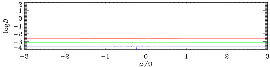
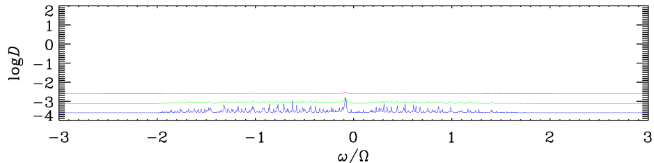
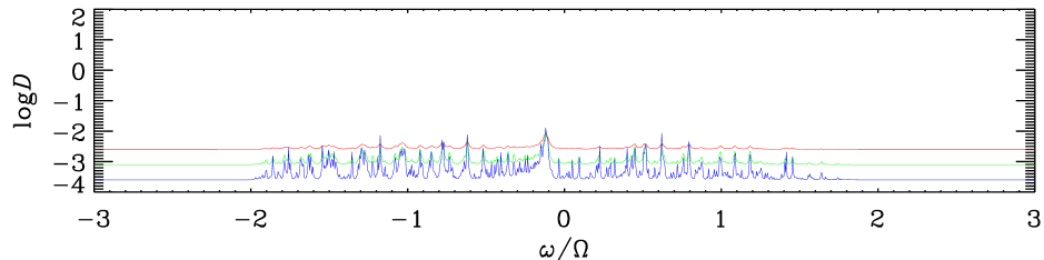
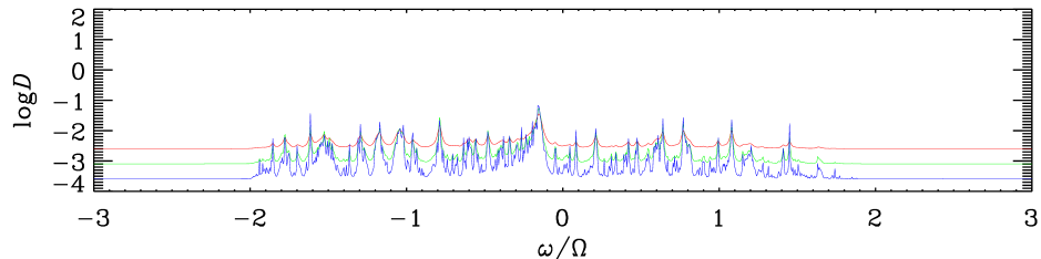
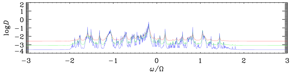
Figure 1: Variation of the total dissipation rate (in units of $\rho R^{3}U^{2}\Omega$) with tidal frequency, for a fluid with a frictional force. The radial velocity is forced at the outer boundary in the form of an $\ell=m=2$ spherical harmonic of amplitude $U$. The fractional core radius is $\alpha=0.1$, $0.2$, $0.3$, $0.4$ and $0.5$ (panels from top to bottom). The frictional damping coefficient $\gamma$ is given by $\gamma/\Omega=10^{-2}$, $10^{-2.5}$ and $10^{-3}$ (red, green and blue curves, from top to bottom for the most part). In all figures, ‘log’ denotes a base-10 logarithm.

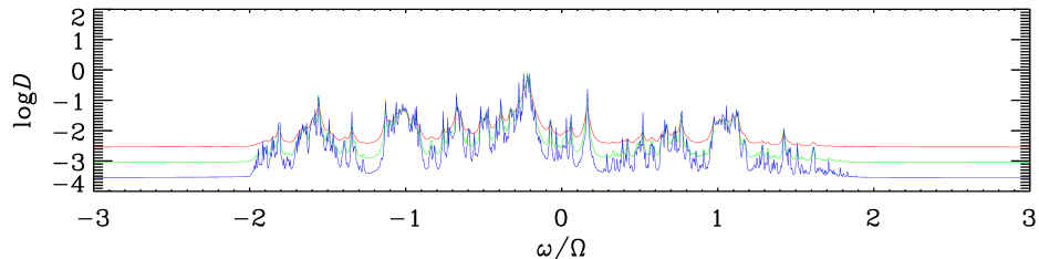
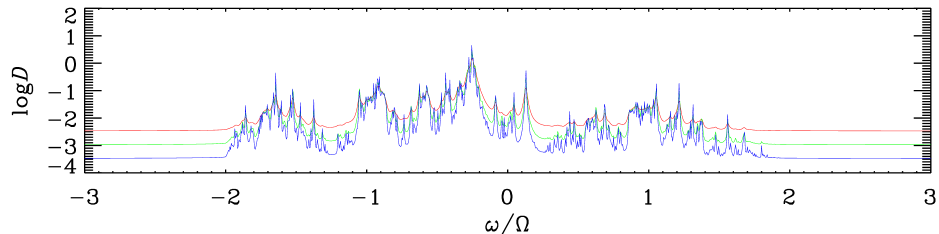
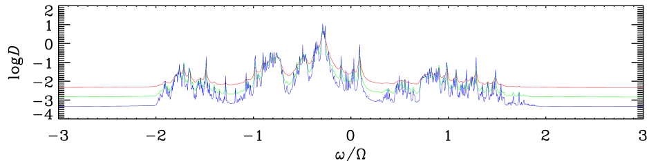
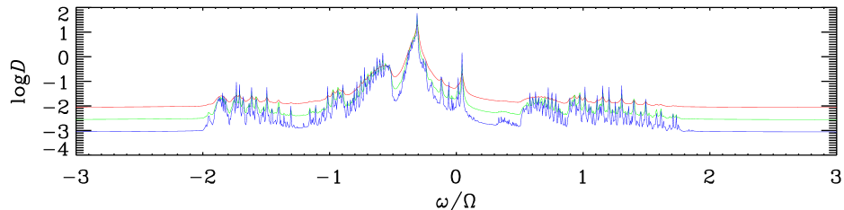
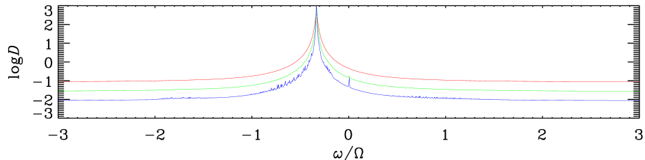
Figure 2: Continuation of Fig. 1 for fractional core radii $\alpha=0.6$, $0.7$, $0.8$, $0.9$ and $0.99$ (panels from top to bottom). Note the different vertical scale in the last case.

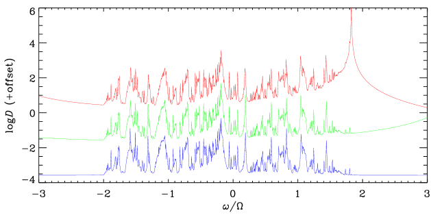
Figure 3: Comparison of tidal and radially forced problems. The bottom (blue) curve shows the total dissipation rate (in units of $\rho R^{3}U^{2}\Omega$) for $\alpha=0.5$ and $\gamma/\Omega=10^{-3}$, as in the bottom panel of Fig. 1. The middle (green) and top (red) curves show the dissipation rate for the tidally forced problem in a planet with dynamical frequency $(g/R)^{1/2}=5\,\Omega$ and $3\,\Omega$, respectively, and with mean density equal to the fluid density. The latter curves are vertically offset by 2 and 4 units, respectively, for clarity. The comparison is made by equating the forced radial velocity amplitude $U$ with $\omega(5/2)(\Psi/g)$.

4.1 Method of solution

We focus on the $\ell=m=2$ type of quadrupolar forcing that is of greatest importance in applications. For the viscous problem, we solve equations (19)–(22) and the appropriate boundary conditions by the pseudospectral method as described in Ogilvie & Lin (2004). This makes use of Chebyshev collocation on a grid of $N+1$ points in $r$ (the Gauss–Lobatto nodes). The system of equations is also truncated at spherical harmonic degree $L$. The problem involves a large block-tridiagonal matrix and the solution is obtained by a standard direct method. The total dissipation rate is computed by two independent methods: from the direct dissipation integral (equation 33) using a Chebyshev quadrature formula, and from the rate of working at the surface (equation 34 or 52 as appropriate).

For the frictional problem, we apply Chebyshev collocation to equation (53) and the appropriate boundary conditions. This has the advantage that the blocks of the tridiagonal matrix are smaller because the other variables have been eliminated in favour of the radial velocity, and therefore a higher resolution can be reached. (In this case the Chebyshev variable is taken to be linearly related to $y$ rather than $r$.)

To validate these methods, we checked that the solutions found by the exponential technique described in Section 3.2, which works very well for modest values of $L$, agree with those obtained by the pseudospectral method. We verified numerically the analytical expressions obtained in Sections 2.5 and 2.6 for the dissipation rate in the non-rotating tidal problem. We also confirmed that the dissipation rates calculated by the integral and surface formulae agree well in all cases.

4.2 Overview of results

In Figs 1 and 2 we present an overview of the behaviour of the dissipation rate with tidal frequency in the radially forced problem with a frictional force, for different values of the fractional core radius $\alpha$ and the frictional damping coefficient $\gamma$. These results were obtained with numerical resolutions of $L=N=200$ or $300$, which is adequate for this kind of overview. A higher resolution is generally required for smaller values of $\gamma$.

Outside the range $-2<\omega/\Omega<2$ the dissipation rate is essentially independent of $\omega$ and proportional to $\gamma$. No inertial waves are excited and the response is smooth and uninteresting. The dissipation rate is greater in a thin shell because of the larger value of the parameter $B$.

Within the range $-2<\omega/\Omega<2$ the dissipation rate is enhanced through the excitation of inertial waves, as found by Ogilvie & Lin (2004). There is a complicated dependence on frequency. In the frequency intervals in which the dissipation rate is most enhanced, it appears to be roughly independent of the frictional damping coefficient.

This enhancement of the dissipation rate increases systematically with the size of the core. In the case of a very thin shell ($\alpha=0.99$), we observe instead a strong resonance with a Rossby wave or r mode at $\omega=-\Omega/3$, as described below.

4.3 Resonance with a Rossby wave or r mode in a thin shell

The limit of a thin shell, $1-\alpha=\epsilon\ll 1$, is of some interest and can be related to problems studied by Laplace (see Lamb, 1932, and references therein). In the absence of viscosity, motions are possible in which, to a first approximation, $a_{n}$ varies linearly with $r$, vanishing at the inner radius, and is much smaller than $rb_{n}$ or $rc_{n}$. Under these circumstances the ‘traditional approximation’ and Laplace’s tidal equations are applicable. In this limit the shell possesses free modes of oscillation which depend on the dimensionless parameter $4\Omega^{2}R^{2}/gh$, where $h=\epsilon R$ is the depth of the ocean (Longuet-Higgins, 1968). When this parameter is much less than unity, simple analytical solutions emerge with frequency $\omega=-2m\Omega/n(n+1)$ for integers $n\geq m$. These are the planetary or Rossby waves, which are well separated from surface gravity waves in the limit under consideration. Related solutions can be identified in stably stratified stellar atmospheres, where they are known as r modes (Papaloizou & Pringle, 1978).

The resonance described above occurs with the $(m=2,n=3)$ Rossby wave or r mode at $\omega=-\Omega/3$. (Note that this is not equivalent to the special, purely toroidal mode discussed in Section 3.3, which has a frequency of $\omega=-2\Omega/3$ and involves no radial motion.) The appropriate balance in equations (21) and (22) is then

$$-\mathrm{i}\omega_{n}c_{n}-2\Omega[(n-1)\tilde{q}_{n}b_{n-1}+(n+2)\tilde{q}_{n+1}b_{n+1}]\approx 0,$$ (61)

$$\frac{\mathrm{d}a_{n}}{\mathrm{d}r}-n(n+1)b_{n}\approx 0.$$ (62)

The boundary conditions determine that $\mathrm{d}a_{n}/\mathrm{d}r=(U/\epsilon R)\delta_{n\ell}$ and we easily obtain $b_{n}$ and $c_{n}$ from the above equations. In the case $\ell=m=2$ investigated here, the toroidal velocity component $c_{3}$ is excited and becomes large when $\omega_{3}$ is small, which occurs close to $\omega/\Omega=-1/3$. The resulting dissipation rate is

$$D\approx\frac{\rho\gamma R^{3}U^{2}}{12\epsilon}\left(1+\frac{32\Omega^{2}}{63|\omega_{3}|^{2}}\right).$$ (63)

This expression provides an excellent fit to the numerically determined dissipation rate in the frictional problem for $\alpha=0.99$. Note that $D$ is inversely proportional to the thickness of the shell. This result occurs because the fast barotropic flow (i.e. horizontal motion independent of depth) excited in a thin shell is efficiently damped by the artificial frictional force in this model; a different behaviour would occur in a viscous fluid. Nevertheless, it is well known from the case of the Earth that highly efficient tidal dissipation can occur in a shallow ocean. The case of the Earth’s ocean is of course enormously complicated by its irregular shape and depth. Mode conversion and turbulence provide channels for dissipation.

4.4 Comparison of tidal and radially forced problems

The original tidal problem, described in Section 2, gives results very similar to those of the simplified, radially forced problem. Some additional parameters are required to set up the tidal problem: the ratio of the dynamical frequency $(g/R)^{1/2}$ to the spin frequency $\Omega$, and the ratio $\beta$ of the fluid density to the mean density of the planet. In Fig. 3 we compare the dissipation rates in the tidal and radially forced problems, with $\alpha=0.5$, $\beta=1$ and $\gamma/\Omega=10^{-3}$. In order to make the comparison we assume that the radial velocity at the surface is determined by equation (27) in the low-frequency limit in which the $W_{n}$ term (and also the viscous term) is neglected. This is equivalent to saying that the radial displacement of the surface is $-(5/2)\Psi/g$, where the factor of $5/2$ comes from the self-gravity of the fluid.

When the planet is slowly rotating, in the sense that $\Omega\ll(g/R)^{1/2}$, the agreement is excellent and shows that the excitation of inertial waves is not affected by the freedom of the outer boundary. For more rapidly rotating planets the influence of surface gravity waves becomes apparent in this range of frequencies. For such rapidly rotating planets the centrifugal distortion of the fluid ought to be taken into account.

4.5 Investigation of a restricted frequency interval

In order to investigate the response in greater detail, we restrict our attention to the case of a fractional core radius $\alpha=0.5$ and to a certain range of frequencies, $1<\omega/\Omega<1.2$. This interval is chosen partly because, as described below, it contains two relatively simple wave attractors. Fig. 4 shows an expanded view of the bottom panel of Fig. 1, using a higher frequency resolution. A higher numerical resolution (up to $L=N=800$) is also used in order to ensure that the results are adequately converged for the appearance of this figure.

Fig. 5 shows equivalent results obtained for a viscous fluid. In this case a smaller numerical resolution (up to $L=N=400$) is achieved and the results are adequately converged except possibly in some cases for the lowest viscosities.

We also show the variation of the dissipation rate with the coefficient of friction or viscosity for three frequencies in this interval, $\omega/\Omega=1.05$, $1.10$ and $1.15$, in Figs 6 and 7. To obtain adequately converged results for the lowest values of $\gamma$ or $\nu$, a very high resolution (up to $L=N=1600$) is required.

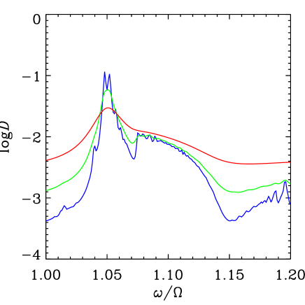
Figure 4: Expanded view of the bottom panel of Fig. 1, i.e. for $\alpha=0.5$ and $\gamma/\Omega=10^{-2}$, $10^{-2.5}$ and $10^{-3}$.

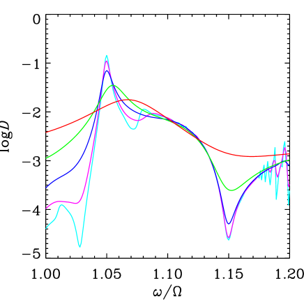
Figure 5: Equivalent of Fig. 4 for a viscous fluid with $\nu/R^{2}\Omega=10^{-4}$, $10^{-5}$, $10^{-6}$, $10^{-7}$ and $10^{-8}$ (red, green, blue, magenta and cyan curves).

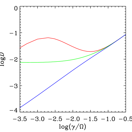
Figure 6: Frictional dissipation versus frictional damping coefficient for $\alpha=0.5$ and $\omega/\Omega=1.05$, $1.10$ and $1.15$ (red, green and blue curves, from top to bottom).

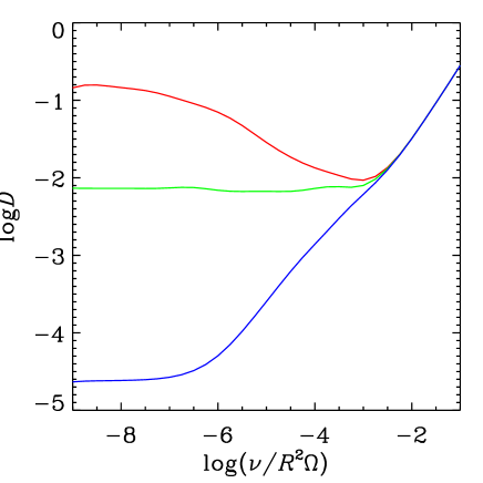
Figure 7: Viscous dissipation versus viscosity for $\alpha=0.5$ and $\omega/\Omega=1.05$, $1.10$ and $1.15$ (red, green and blue curves, from top to bottom).

Perhaps the simplest behaviour occurs close to $\omega/\Omega=1.10$. Here the dissipation rate converges to a non-negligible value as either $\gamma\to 0$ or $\nu\to 0$. The same limiting value is obtained in the frictional and viscous problems and depends smoothly on $\omega$ within a certain interval. This behaviour is closely reminiscent of that found in the analysis of a simple wave attractor (Ogilvie, 2005). We will see below that two distinct types of wave attractor are active in this range of frequencies.

The maximum dissipation rate occurs close to $\omega/\Omega=1.05$. In the frictional problem $D$ does not appear to converge as $\gamma\to 0$, although the ultimate behaviour is not clear from the limited range of parameters that can be investigated numerically. In the viscous problem the dissipation rate gives the appearance of convergence as $\nu\to 0$ but it may decrease below $\nu/R^{2}\Omega=10^{-9}$.

A much lower dissipation rate is found close to $\omega/\Omega=1.15$. Here $D$ appears to converge to a very small value as $\nu\to 0$. It may do so in the frictional problem at lower values of $\gamma$ than are achieved here.

4.6 Spatial structure of the response

We now examine the spatial structure of the response in the meridional plane. Figs 8–10 show the magnitude of the velocity perturbation, $|{\mn@boldsymbol{u}}|$, for frequencies $\omega/\Omega=1.05$, $1.10$ and $1.15$, in the frictional problem with $\gamma/\Omega=10^{-3}$. In each case the disturbance is concentrated near selected inertial-wave rays, which are characteristics of the Poincaré equation.

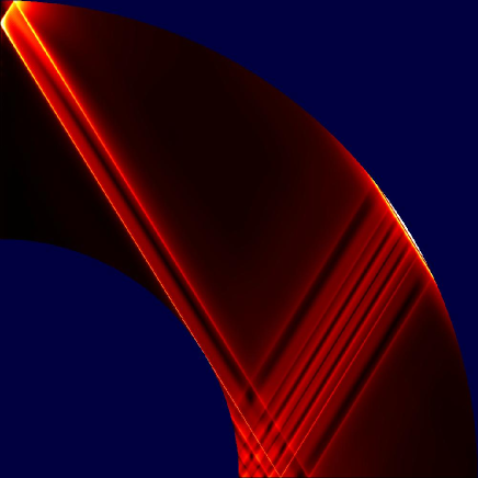
Figure 8: Structure of the velocity perturbation $|{\mn@boldsymbol{u}}|$ in a meridional quarter-plane for the case $\alpha=0.5$, $\omega/\Omega=1.05$, $\gamma/\Omega=10^{-3}$, $L=N=1600$. A linear colour table is used.

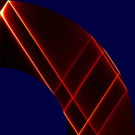
Figure 9: As Fig. 8 but for $\omega/\Omega=1.10$.

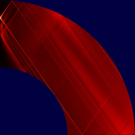
Figure 10: As Fig. 8 but for $\omega/\Omega=1.15$.

Relatively simple wave attractors exist in this range of frequencies. The symmetrical pair of attractors involving four reflections on the outer boundary, illustrated in the upper part of Fig. 11, exists for $1.076<\omega/\Omega<1.148$; a second pair of attractors, involving six outer reflections, exists for $1.091<\omega/\Omega<1.165$. The focusing power of an attractor depends on frequency in a systematic way within the bandwidth of the attractor, as its shape is adapted (Rieutord, Georgeot & Valdettaro, 2001). The first one is strongest at the right-hand end of its bandwidth, while the second is strongest at the left-hand end.

Figure 11: Wave attractors in a spherical annulus with $\alpha=0.5$ at frequency $\omega/\Omega=1.10$.

The response at frequency $1.10$ (Fig. 9) shows that the two types of attractor that exist at this frequency are both activated. The wave energy is concentrated around the attractors in a region whose width is proportional to $\gamma$. This behaviour, and the convergence of the dissipation rate as $\gamma\to 0$ or $\nu\to 0$, are entirely analogous to that found by Ogilvie (2005).

Also seen in this case, however, is a ray emerging from the critical latitude on the inner boundary. This ray is indeed the dominant feature apparent at frequency $1.15$ (Fig. 10) where the dissipation is relatively weak. The attractor with six outer reflections is present in the solution at frequency $1.15$ but is weakly focusing and is not powerfully activated. The dissipation rate in the viscous problem appears to converge to a very low value as $\nu\to 0$ at this frequency.

The behaviour at frequency $1.05$ (Fig. 8), where the dissipation is strongest, is harder to explain. The ray dynamics in the vicinity of this frequency is very complicated. Although extremely long attractors may exist (e.g. one at frequency $1.05$ involving 584 outer reflections) they are of no practical significance. However, there is a tendency for rays to be concentrated temporarily into the region between the equator of the inner boundary and the critical latitude on the outer boundary, where the wave energy is seen to be prominent. The rays escape from this region and reenter it repeatedly. It is difficult to identify features of the ray dynamics that lead to a preference for the frequency $1.05$.

The prominence of rays emerging from the critical latitude on the inner boundary has been noticed before (e.g. Tilgner, 1999; Ogilvie & Lin, 2004).

4.7 Frequency-averaged dissipation rate

There is a strong systematic dependence of the dissipation rate on the size of the core. This effect is examined in Fig. 12, where we plot an average dissipation rate versus $\alpha$. The average is obtained from the data for Figs 1 and 2, by taking the arithmetic mean of the dissipation rates evaluated at 800 equally spaced frequencies in the range $-2<\omega/\Omega<2$. The ‘baseline’ dissipation rate, which occurs for frequencies outside this range, is subtracted from the average, in order to isolate the contribution due to waves. There may be a systematic error in this procedure owing to the inadequate sampling of narrow peaks in the curve.

The resulting values are approximately independent of $\gamma$ and increase approximately as the fifth power of the core radius. Interestingly, this dependence is predicted by the recent analysis of Goodman & Lackner (2008), who consider the scattering of the equilibrium tide off the core, although they do not predict the intricate variation with frequency. A departure from this behaviour occurs as $\alpha$ approaches $1$, owing to the toroidal-mode resonance in a thin shell.

Figure 12: Estimates of the frequency-averaged dissipation rate over the interval $-2<\omega/\Omega<2$, minus the ‘baseline’ dissipation outside this range, versus fractional core radius, for the frictional problem with $10^{-3}\leq\gamma/\Omega\leq 10^{-2}$. The dotted line represents $0.11\alpha^{5}$.

5 Discussion

5.1 Interpretation of enhanced dissipation

The dynamics of inertial waves in a spherical annulus is very rich and a great deal remains to be explained. In earlier work (Ogilvie, 2005) we considered a simpler type of domain in which all wave energy is focused towards a single wave attractor and a dissipation rate is obtained that is asymptotically independent of the viscosity or other small-scale damping mechanism for the waves. In a spherical annulus, the closest parallel to this behaviour occurs in situations such as that illustrated in Fig. 9, although in fact more than one attractor is activated there. The spherical annulus is more complicated because simple attractors occupy only a limited range of frequencies, and also because of the existence of a critical latitude at which rays are tangent to the inner boundary. In fact these features are related to each other, because the range of frequencies in which an attractor exists is bounded by situations in which its rays approach the critical latitude on the inner and outer boundaries (Rieutord, Georgeot & Valdettaro, 2001).

Both attractors and critical latitudes concentrate wave energy and promote enhanced dissipation. A smooth beam of waves reflecting from the inner boundary generates a singularity in an inviscid fluid, as illustrated in Fig. 13. This effect depends smoothly on frequency in the range $-2<\omega/\Omega<2$. When the singular beam emanating from the critical latitude is resolved by viscosity, enhanced dissipation occurs but this alone does not account for the behaviour seen close to $\omega/\Omega=1.05$ in Fig. 5; it is more suitable as an explanation of the behaviour close to $\omega/\Omega=1.00$, where $D$ scales approximately with $\nu^{1/2}$.

Figure 13: Formation of a singularity at the critical latitude through the reflection of rays (equally spaced lines incident from the top right) from the inner boundary.

The behaviour of rays alone is not sufficient to explain the shape of the dissipation curve. This can be seen from the fact that $D$ depends on the sign of $\omega/\Omega$ and on the value of $m$ (not shown here), whereas the rays are insensitive to these properties. Even in the case of a simple wave attractor, the full calculation of the asymptotic dissipation rate depends on a detailed analysis of the forcing accumulated around each ray circuit (Ogilvie, 2005).

Some time after the calculations described in this paper were completed, we received a preprint from Goodman & Lackner (2008). They treat the equilibrium tide as a large-scale inertial wave that reflects from the inner boundary. The intense beam emanating from the neighbourhood of the critical latitude produces enhanced dissipation, occurring in their analysis through nonlinearity. This theory has an attractive simplicity to it and appears to predict the correct scaling of the frequency-averaged dissipation rate on the size of the core. It does not predict a complicated frequency-dependence because further reflections are not considered. Indeed, as is mentioned below, the various physical circumstances in planets and stars may not always permit the multiple reflections that occur in the simple model considered in the present paper.

After this paper was submitted, we also received a manuscript from M. Rieutord and L. Valdettaro, who have considered a similar problem and have been able to relate some aspects of the frequency-dependence of the dissipation rate to the properties of wave attractors, viscous normal modes and critical latitudes.

5.2 Astrophysical and planetary applications

The dissipation rates $D$ (expressed in units of $\rho R^{3}U^{2}\Omega$) plotted in various figures in this paper can be converted into modified tidal quality factors $Q^{\prime}$ according to the relation

$$\frac{1}{Q^{\prime}}=\frac{4}{5}\beta(1-{\textstyle\frac{3}{5}}\beta)^{-2}\frac{\Omega|\omega|}{g/R}\left(\frac{D}{\rho R^{3}U^{2}\Omega}\right).$$

For a fixed value of $\omega/\Omega$ in the range of inertial waves, the efficiency of tidal dissipation through this mechanism therefore scales with the square of the ratio of the spin frequency to the dynamical frequency of the body (Ogilvie & Lin, 2004). This fact should always be borne in mind when comparing solar system planets with hot Jupiters and hot Neptunes, which are expected to rotate more slowly as a result of tidal evolution. The wide variation in $D$ indicates that a very broad range of $Q^{\prime}$ values can occur through this mechanism. The strong frequency-dependence of $Q^{\prime}$ can have important consequences for tidal evolution, for example in shaping the satellite systems of the giant planets.

We note that the tidal quality factor provides only a conventional and, for some purposes, convenient parametrization of the efficiency of tidal dissipation, which can involve complicated processes of wave excitation, propagation and damping. It depends as much on the capacity of the system to respond to oscillatory forcing as on its ability to dissipate the response.

5.3 Topics for further investigation

The problem studied in this paper is intentionally simplified in order to try to isolate an already complicated physical process. We mention here some of the topics that require further investigation.

The quality of wave reflection from the boundaries of the fluid region supporting inertial waves should be analysed. Depending on the type of planet or star being considered, these boundaries may be free surfaces, interfaces with solid or denser fluid material, or borders between convective and radiative zones. Internal reflection of inertial waves from discontinuities such as a putative first-order phase transition in giant planets are also potentially of importance.

The propagation of inertial waves could be affected by differential rotation, magnetic fields, buoyancy effects and the centrifugal distortion of the body. It would also be of interest to study an initial-value problem rather than assuming a response that is harmonic in time.

Dissipation mechanisms for inertial waves at small scales include viscous damping, interaction with turbulent convection, Ohmic dissipation through coupling with magnetic fields, and nonlinear dissipation through wave breaking or parametric instability. While the analysis of a simple wave attractor indicated a total dissipation rate that is asymptotically independent of the small-scale processes, a more complicated picture arises from the present paper and it may be necessary to understand the damping mechanisms in greater detail.

The dependence of the dissipation rate on the size of the core should be investigated in more realistic models where the fluid is compressible and the core is deformable. The role of resonances with global normal modes (if they exist) in compressible models needs to be clarified. The relevance of boundary layers on the surface of the core, obviated here through the use of stress-free boundary conditions, is worthy of consideration. Dissipation within the core itself is yet another area of uncertainty.

5.4 Elliptical instability

A quite different paradigm for tidal dissipation in rotating planets and stars could emerge through a consideration of elliptical instabilities (Kerswell, 2002, and references therein). If the linear tidal response is considered to provide merely an elliptical distortion of the streamlines of the rotating fluid, as is true in the case of a full sphere of incompressible fluid, then the secondary instabilities of the elliptical flow can produce turbulence and enhanced tidal dissipation. Analytical, numerical and experimental investigations have been motivated mainly by the case of the Earth’s core but also by Io (Kerswell & Malkus, 1998) and by accretion discs in binary stars (Goodman, 1993; Lubow, Pringle & Kerswell, 1993; Ryu & Goodman, 1994). This nonlinear mechanism may be more relevant for tides in extrasolar planets, while the much weaker tides in solar-system planets may depend on linear mechanisms such as those described in this paper. Since the linear response in a spherical annulus departs significantly from a simple elliptical distortion, it would be of interest to understand the nonlinear outcome in the presence of a core.

6 Conclusion

In this paper we have studied the tidal forcing, propagation and dissipation of linear inertial waves in a rotating fluid body. The intentionally simplified model involves a perfectly rigid core surrounded by a deep ocean consisting of a homogeneous incompressible fluid. Centrifugal effects are neglected, but the Coriolis force is considered in full, and dissipation occurs through viscous or frictional forces. We introduced a further simplification by replacing the free outer surface with a boundary on which the radial velocity is specified, which closely mimics the effects of tidal forcing at low frequencies. Various analytical results provide tests of the numerical methods for calculating forced linear waves.

The dissipation rate exhibits a complicated dependence on the tidal frequency and generally increases strongly with the size of the core. In certain intervals of frequency, efficient dissipation is found to occur even for very small values of the coefficient of viscosity or friction, which is promising for astrophysical and planetary applications. In restricted intervals, the wave energy is focused towards relatively simple wave attractors and a well defined asymptotic dissipation rate is achieved. However, a more typical behaviour is that the inertial waves propagate in a very complicated way around the fluid annulus. The critical latitude on the inner boundary plays an important role in the solutions. While the dissipation rate is enhanced in a strongly frequency-dependent manner, it may not converge in the limit of small viscosity in the same way as for a wave attractor. In the limit of a thin fluid shell, the dissipation rate can be greatly enhanced through a traditional type of resonance with a toroidal mode (r mode or Rossby wave).

The model adopted in this paper is deliberately oversimplified, although it may be more or less applicable to planets or moons involving a deep ocean. We have pointed out numerous avenues for further investigation, including aspects of internal wave propagation, reflection and dissipation, and nonlinear behaviour such as the elliptical instability.

acknoweldgments

I thank Jeremy Goodman and the referee, Leo Maas, for helpful comments.

References

- Goldreich & Keeley (1977) Goldreich P., Keeley D. A., 1977, ApJ, 211, 934
- Goldreich & Nicholson (1977) Goldreich P., Nicholson P. D., 1977, Icarus, 30, 301
- Goldreich & Nicholson (1989) Goldreich P., Nicholson P. D., 1989, ApJ, 342, 1079
- Goldreich & Soter (1966) Goldreich P., Soter S., 1966, Icarus, 5, 375
- Goodman (1993) Goodman J., 1993, ApJ, 406, 596
- Goodman & Dickson (1998) Goodman J., Dickson E. S., 1998, ApJ, 507, 938
- Goodman & Lackner (2008) Goodman J., Lackner C., 2008, arXiv, arXiv:0812.1028
- Goodman & Oh (1997) Goodman J., Oh S. P., 1997, ApJ, 486, 403
- Greenspan (1968) Greenspan H. P., 1968, The Theory of Rotating Fluids, Cambridge Univ. Press, Cambridge
- Ivanov & Papaloizou (2007) Ivanov P. B., Papaloizou J. C. B., 2007, MNRAS, 376, 682
- Kerswell (2002) Kerswell R. R., 2002, Ann. Rev. Fluid Mech., 34, 83
- Kerswell & Malkus (1998) Kerswell R. R., Malkus W. V. R., 1998, Geophys. Res. Lett., 25, 603
- Lamb (1932) Lamb H., 1932, Hydrodynamics, 6th edn, Cambridge Univ. Press, Cambridge, §213
- Longuet-Higgins (1968) Longuet-Higgins M. S., 1968, RSPTA, 262, 511
- Lubow, Pringle & Kerswell (1993) Lubow S. H., Pringle J. E., Kerswell R. R., 1993, ApJ, 419, 758
- Lubow, Tout & Livio (1997) Lubow S. H., Tout C. A., Livio M., 1997, ApJ, 484, 866
- Maas et al. (1997) Maas L. R. M., Benielli D., Sommeria J., Lam F.-P. A., 1997, Nature, 388, 557
- Manders & Maas (2003) Manders A. M. M., Maas L. R. M., 2003, J. Fluid Mech., 493, 59
- Ogilvie (2005) Ogilvie G. I., 2005, J. Fluid Mech., 543, 19
- Ogilvie & Lin (2004) Ogilvie G. I., Lin D. N. C., 2004, ApJ, 610, 477
- Ogilvie & Lin (2007) Ogilvie G. I., Lin D. N. C., 2007, ApJ, 661, 1180
- Papaloizou & Ivanov (2005) Papaloizou J. C. B., Ivanov P. B., 2005, MNRAS, 364, L66
- Papaloizou & Pringle (1978) Papaloizou J., Pringle J. E., 1978, MNRAS, 182, 423
- Papaloizou & Savonije (1997) Papaloizou J. C. B., Savonije G. J., 1997, MNRAS, 291, 651
- Penev et al. (2007) Penev K., Sasselov D., Robinson F., Demarque P., 2007, ApJ, 655, 1166
- Rieutord (1991) Rieutord M., 1991, Geophys. Astrophys. Fluid Dyn., 59, 185
- Rieutord, Georgeot & Valdettaro (2001) Rieutord M., Georgeot B., Valdettaro L., 2001, J. Fluid Mech., 435, 103
- Rieutord & Valdettaro (1997) Rieutord M., Valdettaro L., 1997, J. Fluid Mech., 341, 77
- Ryu & Goodman (1994) Ryu D., Goodman J., 1994, ApJ, 422, 269
- Savonije & Papaloizou (1983) Savonije G. J., Papaloizou J. C. B., 1983, MNRAS, 203, 581
- Savonije & Papaloizou (1984) Savonije G. J., Papaloizou J. C. B., 1984, MNRAS, 207, 685
- Savonije & Papaloizou (1997) Savonije G. J., Papaloizou J. C. B., 1997, MNRAS, 291, 633
- Savonije, Papaloizou & Alberts (1995) Savonije G. J., Papaloizou J. C. B., Alberts F., 1995, MNRAS, 277, 471
- Savonije & Witte (2002) Savonije G. J., Witte M. G., 2002, A&A, 386, 211
- Terquem et al. (1998) Terquem C., Papaloizou J. C. B., Nelson R. P., Lin D. N. C., 1998, ApJ, 502, 788
- Tilgner (1999) Tilgner A., 1999, PhRvE, 59, 1789
- Verbunt & Phinney (1995) Verbunt F., Phinney E. S., 1995, A&A, 296, 709
- Witte & Savonije (1999) Witte M. G., Savonije G. J., 1999, A&A, 341, 842
- Wu (2005a) Wu Y., 2005a, ApJ, 635, 674
- Wu (2005b) Wu Y., 2005b, ApJ, 635, 688
- Zahn (1966a) Zahn J. P., 1966a, AnAp, 29, 313
- Zahn (1966b) Zahn J. P., 1966b, AnAp, 29, 489
- Zahn (1970) Zahn J. P., 1970, A&A, 4, 452
- Zahn (1975) Zahn J.-P., 1975, A&A, 41, 329
- Zahn (1977) Zahn J.-P., 1977, A&A, 57, 383