A tensor theory of space-time as a strained material continuum

Abstract

The classical theory of strain in material continua is reviewed and generalized to space-time. Strain is attributed to "external" (matter/energy fields) and intrinsic sources fixing the global symmetry of the universe (defects in the continuum). A Lagrangian for space-time is worked out, adding to the usual Hilbert term an "elastic" contribution from intrinsic strain. This approach is equivalent to a peculiar tensor field, which is indeed part of the metric tensor. The theory gives a configuration of space-time accounting both for the initial inflation and for the late acceleration. Considering also the contribution from matter the theory is used to fit the luminosity data of type Ia supernovae, giving satisfactory results. Finally the Newtonian limit of the theory is obtained.

1 Introduction

There are in cosmology a limited but important number of facts which do not fit in the classical general relativistic (GR) frame of the standard theory. Among others we recall the current accelerated expansion of the universe, as discovered at the end of 1998 observing the redshift dependence of the luminosity of type Ia supernovae [1, 2], the extreme uniformity of the temperature of the Cosmic Microwave Background (CMB) [3, 4, 5], the anomalous rotation curves of spiral galaxies [6, 7], the anomalous mass-luminosity relation in galaxy clusters [8] and the galaxy power spectra [9]. If, on one side, the number of facts to be accounted for is limited, on the other, the number of theories put forth to explain them is extremely high. All these theories may however be grouped under a limited number of headings. One is GR plus appropriate fields. We may include in this category the inflaton, accounting for the homogeneity of the CMB [10, 11, 12], as well as quintom [13, 14], k-essence [15, 16] and vector inflation [17]. Then we find dark energy in a number of variants: cosmological constant [18, 19, 20, 21], quintessence[22, 23], phantom energy [24, 25], holographic dark energy [26, 27, 28], triads [29] and k-essence again [30]. Together with the idea of dark energy we may quote an, in principle, different ingredient of the universe which is dark matter[31]; now the competition opens among many possible types of non-baryonic matter and specific candidates: Hot Dark Matter [32], which actually seems not to be the right stuff since it does not allow for structure formation; Cold Dark Matter [33]; Warm Dark Matter [34]; neutrinos, gravitinos, photinos, axions, sterile neutrinos, Weakly Interacting Massive Particles (WIMPS), Lightest Supersymmetric Particles (LSP). By the way the most successful cosmological theory of the moment is the so called Lambda-Cold Dark Matter theory ($\Lambda CDM$) [35]

Another compartment is the one of extended, alternative, modified theories of gravity (all changes are with respect to standard GR). In this group we find both metric and Palatini versions of $f\left(R\right)$ theories [36, 37] and Modified Newtonian Dynamics (MOND) [38, 39, 40] and its covariant formulation [41].

All these possibilities remain within the realm of classical theories, but of course we have also a host of attempts to introduce quantum aspects in a more or less fundamental way. So we find various string cosmologies [42], brane world [43], Loop Quantum Cosmology [44, 45], and similar approaches.

Everything can be good or not according to the capability of one or another idea to account for a consistent enough number of facts, which, as said, are rather few. The impression one has, however, is that most theories rely much more on the mathematics of the model rather than on physics. In some cases we have more or less explicit tricks introduced in order to produce the right equations. The wording is in any case physical, but the entities that are called in often have rather exotic properties, in the sense that they are completely unusual, i.e. not corresponding to anything else we know. So, considering the various entities that are introduced in the universe in order to account for the accelerated expansion we have "fluids" which do not dilute even though the available room is increasing (cosmological constant), violating the strong energy condition (quintessence), such that when compressed they expand (phantom energy). Mathematically everything is OK but someone may feel uneasy with all that belonging to the actual world.

In order to find a route in the wild forest of conjectures one needs a criterion and one could be to stick, as far as possible, to the physical properties one already knows and has learned to describe. Of course there is no reason why the universe on the largest scale should possess properties that look like the ones we are used to at everyday’s scale, but we have some hints telling us that this approach could be not completely absurd. On one side we know that the world becomes richer at the tiniest scales than at our usual scale: wave functions and the whole machinery of quantum mechanics are not needed to describe the world at the human scale. On another side we know that some properties of complex systems are scale invariant. On this more or less inspiring basis we have tried to draw on a known methodology and a known theory in order to describe space-time as such. In GR space-time is indeed described as a real continuum which interacts with something else, being this "something else" what we call matter/energy; the interaction is expressed by the non-linear Einstein equations whereby the non-linearity implies that space-time, in a sense, interacts also with itself. Following on we easily see that many techniques used for space-time in GR are very similar to the ones applied to describe material continua in the theory of elasticity: in the end, in both cases, everything is dominated by geometry. How far this analogy can go? How the basic tools of the elasticity theory need be modified in order to fit the behaviour of a four-dimensional manifold with Lorentzian signature? The idea is not at all new and in a sense has distant roots even in the old investigations on the nature of the "luminiferous ether" that haunted physics until the beginning of the XXth century. Of course the "ether" was thought of as something filling space and moving or vibrating in an absolute time, the mathematical tools and concepts were the ones of the XIX century and the aim of the research was the explanation of the propagation of light. However, as we know, after getting rid of the name "ether" Einstein remarked (1920) that "…space is endowed with physical qualities; in this sense, therefore, there exists an ether…" [46], and in today’s quantum field theories the ether is named "the vacuum" and has indeed important physical properties. So what we are about to do is to explore the idea of space-time as a material continuum using the formalism and general framework of GR and the leading idea of the material continua we know. The central concept will be the strain of the four-dimensional manifold which is related to the metric tensor and is in turn produced by some cause. The origin of the strain can be either "external" or internal and in our case, according to the universally adopted dualistic approach, "external" will mean matter/energy. The possibility of internal or spontaneous strain states is well known in the theory of elasticity and plasticity and is connected with the presence of structural defects in the "texture" of the manifold. So the other concept we shall use in our theory will be the one of space-time defect or Cosmic Defect (CD) which we use also to name the theory.

We have already applied this approach heuristically to the interpretation of the late acceleration of the universe, obtaining encouraging results [47, 48]. Here we are giving a new formulation of the theory, casting it in a systematic and general way.

2 Review and reformulation of the metric properties of elastic continua

For our purposes we shall consider an $N-$dimensional material continuum and assume that in its reference state it is perfectly homogeneous and isotropic so that we may identify it with an $N-$dimensional Euclidean manifold (reference manifold) [49, 50].

If we now imagine to apply some action (in three dimensions we would speak of forces) either localized or diffused, we expect the continuum to be brought to a deformed (strained) state, where in general it, as a manifold, will acquire curvature: this will be our "natural" manifold [50].

Let us then imagine we have two copies of the system, one in the reference state, the other in the natural one, and that they are both embedded in an $N+1$ - dimensional simply-connected flat Minkowskian manifold ; the additional dimension will be time-like. We consider a situation in which it is possible to put in one to one correspondence points on the two manifolds. This operation may be formally thought of as a type II gauge transformation [52, 53].

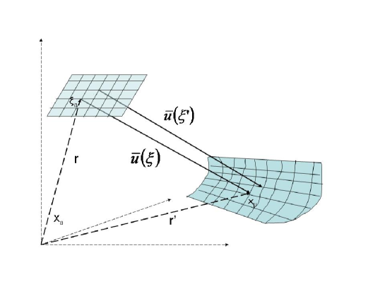
Figure 1: Embedding of the reference and the natural manifolds in an $N+1$ - dimensional flat manifold. $X_{a}$ are the Cartesian coordinates in the embedding manifold; $\xi_{\mu}$ are the coordinates on the reference (sub)-manifold ($N$ - dimensional), $x_{\nu}$ are the coordinates in the natural (generally curved) (sub)-manifold. $u$ represents the displacement vector from points of the reference manifold to points of the natural manifold.

Considering the embedding $N+1$ - manifold we may introduce a "displacement vector field" $u$ which connects pairs of points in the two embedded $N$ -dimensional manifolds. If $r$ is the $N+1$- vector localizing a point in the reference manifold, the $u$ vector runs from that position to a different one $r^{\prime}$ in the natural manifold. The situation is shown on fig.( 1). $X$’s are the (Cartesian) coordinates of the embedding manifold; the coordinates on the reference manifold are $\xi$’s; the ones of the natural manifold are $x$’s. We assume that the functional dependences leading from one coordinate system to the other are all sufficiently smooth for the rest of our reasoning to be valid. Of course the different dimensionality implies the existence of at least one constraint for each of the two sub-manifolds allowing for the dimensional reduction. In general we assume $\xi_{\mu}=f_{\mu}\left(X_{1},...,X_{N+n}\right)$ and (on the reference sub-manifold) $X_{i}=h_{i}\left(X_{1},...,X_{N}\right)$ for $i=N+1,...,N+n$ ; the same holds for the natural manifold: $x_{\alpha}=w_{\alpha}\left(X_{1},...,X_{N+n}\right)$ and $X_{i}=q_{i}\left(X_{1},...,X_{N}\right)$ for $i=N+1,...,N+n$. If all functions are differentiable and invertible one can also write:

$$x_{\mu}=m_{\mu}\left(\xi_{1},...,\xi_{N}\right)$$ (1)

On these bases we may write, with reference to the embedding manifold:

$$r^{\prime}\left(X\right)=r\left(X\right)+u\left(X\right)$$ (2)

The functions $f$ and $w$ together with the constraints allow to cast (2) in terms of the reference $\{\xi\}$ or natural $\{x\}$ coordinates. A choice one can always do is to numerically identify $\xi$’s and $x$’s for corresponding places in the two manifolds, not forgetting that this choice can be practically useful but has per se no physical meaning.

Everything is non-trivial only in the case of $u$ being a non-trivial field: rigid translations are uninteresting and amount to a simple coordinate change in the same manifold.

The next step we may think to do is to compare the distances between pairs of corresponding points in the unstretched and stretched situations. This comparison is meaningful only if made in one and a single manifold, i.e. the embedding one. Using unprimed symbols for the reference manifold and primed symbols for the natural one we may write

$$\begin{array}[]{l}dl^{2}=\eta_{ab}dX^{a}dX^{b}\\ dl^{\prime 2}=\eta_{ab}dX^{\prime a}dX^{\prime b}\end{array}\quad\quad a,b=1,...,N+n$$

In both cases the metric tensor is the one pertaining to the flat embedding manifold. Introducing the constraints defining the two sub-manifolds of interest and using the coordinates adopted for each of them, the equations above become

$$\begin{array}[]{lll}dl^{2}=&\eta_{ab}\frac{\partial X^{a}}{\partial\xi^{\mu}}\frac{\partial X^{b}}{\partial\xi^{\nu}}d\xi^{\mu}d\xi^{\nu}=&\eta_{\alpha\beta}d\xi^{\alpha}d\xi^{\beta}=\mathsf{\eta}_{\mu\nu}dx^{\mu}dx^{\nu}\\ dl^{\prime 2}=&\eta_{ab}\frac{\partial X^{\prime a}}{\partial x^{\mu}}\frac{dX^{\prime b}}{\partial x^{\nu}}dx^{\mu}dx^{\nu}=&g_{\mu\nu}dx^{\mu}dx^{\nu}\\ \end{array}\qquad\quad\mu,\nu=1,...,N$$

Saturation of the Latin indices leads, on the first row, to the $N$ -dimensional flat metric tensor of the reference manifold (either Euclidean or Minkowskian); however it is important to stress that the additional factors $\partial\xi^{\alpha}/\partial x^{\mu}$ do not correspond to a coordinate change on the same manifold, so that the final $\mathsf{\eta}_{\mu\nu}$ tensor is not in general a metric tensor on the natural manifold. Viceversa on the second line, the constraint to stay on the natural manifold leads in general to a curved $N$ - dimensional metric (with Lorentzian signature). Using (2) and (1) we see that it is:

$$g_{\mu\nu}\left(x\right)=\mathsf{\eta}_{\mu\nu}+2\varepsilon_{\mu\nu}\left(x\right)$$ (3)

where $\varepsilon_{\mu\nu}$ is the strain tensor of the natural manifold, given by

$$\varepsilon_{\mu\nu}=\frac{1}{2}\left(\eta_{a\mu}\frac{\partial u^{a}}{\partial x^{\nu}}+\eta_{\nu b}\frac{\partial u^{b}}{\partial x^{\mu}}+\eta_{ab}\frac{\partial u^{a}}{\partial x^{\mu}}\frac{\partial u^{b}}{\partial x^{\nu}}\right)$$ (4)

Looking at (4) we easily see that the strain we have defined transforms as a genuine tensor on the natural four-dimensional manifold.
If one could find a coordinate transformation such that (3) could be written as

$$g_{\mu\nu}=\eta_{\alpha\beta}\frac{\partial\xi^{\alpha}}{\partial x^{\mu}}\frac{\partial\xi^{\beta}}{\partial x^{\nu}},$$ (5)

then the strained and the unstrained situations would be diffeomorphic to each other ($\mathsf{\eta}_{\mu\nu}$ would coincide with $g_{\mu\nu}$) and it would be impossible to perceive the deformation from within the manifold: no intrinsic curvature. In fact the integrability condition for (5) is De Saint Venant’s:

$$R_{\beta\gamma\delta}^{\alpha}=0,$$ (6)

where $R_{\beta\gamma\delta}^{\alpha}$ are the components of the Riemann tensor. This is indeed the case of elastic deformations, which have an exogenous origin: they are due to the application of external forces and the strain is brought to zero whenever those forces are removed (absence of plastic deformations). In practice a smooth and continuous $u$ field leads to an integrable (5). If we are interested in intrinsic deformations (the ones that can be sensed from within) we must study singular $u$ (and $\varepsilon$) fields, the singularity being represented by some discontinuity in $u$ and/or its derivatives. Now, a singular displacement field in a continuum means that the medium contains what is formally defined as one defect (or more), according to the definition given by Volterra in 1907, while studying elastic and plastic deformations [54].

The singularity in $u$ reflects of course also in the strain tensor and in general we shall write [55, 56, 57] the elementary deformation (from (2) in the reference frame) as a non integrable one form:

$$dr^{\prime\mu}=\omega_{\nu}^{\mu}dr^{\nu},$$

so that the deformed line element will be

$$ds^{2}=g_{\mu\nu}\left(x\right)dx^{\mu}dx^{\nu}=\eta_{\alpha\beta}\omega_{\lambda}^{\alpha}\omega_{\rho}^{\beta}d\xi^{\lambda}d\xi^{\rho}$$

Now, our target is space-time and we know that interesting situations there imply condition (6) to be violated so that we are led to the conclusion that any non-trivial space-time should contain at least one defect in the sense recalled above. This is a different way to the singularity theorems by Hawking and Penrose [58]. A warning that is appropriate to issue at this point is that the defect we are considering here should not be confused with the topological ones often appearing in cosmology. There the topological defects are the residual of the phase transition which gave origin to matter during inflation. Of course "our" defects also have topological properties, however their nature is completely different, as we have seen.

3 Lagrangians for space-time

After the geometric considerations developed in the previous section we are left with the problem of finding the functional dependence of $u$ (or to say better, $\varepsilon$) on the coordinates. In practice this means that we need to introduce an appropriate Lagrangian for our space-time manifold.

Let us start from the typical Einstein-Hilbert Lagrangian for a defectless manifold

$$L_{EH}=R\sqrt{-g},$$ (7)

which is build from the simplest scalar obtainable from the curvature tensor. We of course expect that the Lagrangian we are looking for reduces to (7) when the defect disappears. An apparently reasonable approach is to add to (7) an "elastic" potential term: this would be consistent with the description given so far.

A typical expression for the elastic potential energy is:

$$W_{e}=\frac{1}{2}\sigma_{\mu\nu}\varepsilon^{\mu\nu}$$ (8)

where the usual meaning of $\sigma_{\mu\nu}$ is to be the components of the stress tensor of the material. The stress is naturally dependent on the strain and viceversa. In the standard elasticity theory this dependence is mostly dealt with assuming a linear relation (Hooke’s law) [49]. In the case of space-time we have a priori no reason to say that it is so also, but we shall assume linearity and see what happens. We write:

$$\sigma_{\mu\nu}=C_{\mu\nu\alpha\beta}\varepsilon^{\alpha\beta}$$

where $C_{\alpha\beta\mu\nu}$ are the components of the elastic modulus tensor and are supposed to be independent from the $\varepsilon$’s. As a consequence (8) becomes:

$$W_{e}=\frac{1}{2}C_{\mu\nu\alpha\beta}\varepsilon^{\alpha\beta}\varepsilon^{\mu\nu}$$ (9)

We have of course to do with a scalar density and we may study the situation in a locally flat manifold (tangent space). Assuming that the medium, at least in the unperturbed condition, is perfectly homogeneous and isotropic the form assumed by the elastic modulus tensor depends on two parameters only [49] and is

$$C_{\alpha\beta\gamma\delta}=\lambda\eta_{\alpha\beta}\eta_{\gamma\delta}+\mu\left(\eta_{\alpha\gamma}\eta_{\beta\delta}+\eta_{\alpha\delta}\eta_{\beta\gamma}\right)$$ (10)

The parameters $\lambda$ and $\mu$ are known as the Lamé coefficients; their value is a property of the continuum under consideration. In the standard elasticity theory instead of the $\eta$’s one has Kronecker deltas (at least for Cartesian coordinates), i.e. the Euclides metric tensor; here we introduce the Minkowski tensor, because we are dealing with space-time. In the case of space-time the global isotropy condition in four dimensions has to be taken with caution, because of the light cones, however we shall assume it holds. Considering (10) and (9) we arrive at

$$W_{e}=\left(\frac{1}{2}\lambda\varepsilon^{2}+\mu\varepsilon_{\alpha\beta}\varepsilon^{\alpha\beta}\right)$$

being $\varepsilon=\varepsilon_{\alpha}^{\alpha}$ the trace of the strain tensor. In the globally curved manifold the corresponding Lagrangian density is:

$$L_{e}=\left(\frac{1}{2}\lambda\varepsilon^{2}+\mu\varepsilon_{\alpha\beta}\varepsilon^{\alpha\beta}\right)\sqrt{\left|g\right|}$$ (11)

Of course indices are raised and lowered by means of the global metric tensor.

The complete action integral for the natural manifold (no external forces: in practice no matter, in our case) will be:

$$\int\left(R+\frac{1}{2}\lambda\varepsilon^{2}+\mu\varepsilon_{\alpha\beta}\varepsilon^{\alpha\beta}\right)\sqrt{\left|g\right|}dx^{N}$$ (12)

The structure of (12) recalls the classical form where a kinetic and a potential terms appear. Here the role of kinetic term is played by $R$ which contains derivatives of the strain tensor.

3.1 "Elastic" Einstein equations

The treatment we have given of the behaviour of the "elastic-style" space-time is not different in the form from the introduction of some "material" contribution to the Lagrangian. Now this contribution is expressed by (11) with

$$\varepsilon_{\mu\nu}=\frac{1}{2}\left(g_{\mu\nu}-\mathsf{\eta}_{\mu\nu}\right).$$ (13)

One has to be careful in dealing with $\mathsf{\eta}_{\mu\nu}$. As already said, this is a tensor on the natural manifold, but is no metric at all for that manifold. The $\mathsf{\eta}_{\mu\nu}$ tensor can in practice be identified with the metric of the local tangent four-dimensional frame, comoving with the cosmic flow of the given universe. At different cosmic times the various local $\mathsf{\eta}_{\mu\nu}$ tensors are related to each other via boosts based on the expansion rate.

In principle from (11) and using (13), varying the action integral with respect to $g_{\mu\nu}$ (or equivalently $\varepsilon_{\mu\nu}$ which is proportional to the non trivial part of the metric tensor), we may obtain generalized Einstein equations in the form:

$$G_{\mu\nu}=T_{e\mu\nu}+\kappa T_{\mu\nu}$$ (14)

where all that is neither in the Einstein tensor nor in the matter energy-momentum tensor can be interpreted as an effective "elastic" energy momentum tensor $T_{e\mu\nu}$. Since $T_{e\mu\nu}$, as well as $T_{\mu\nu}$, is obtained varying a true scalar (the integrand of (12)) with respect to a true tensor, it is also a good tensor, retaining all properties of tensors. In particular no coordinate choice can bring $T_{e\mu\nu}$ to zero, unless it is identically zero.

In vacuo the final matter term is absent, however now it is in general $R\neq 0$, provided some internal cause, like a defect, is there. The tensor $T_{e\mu\nu}$, though being partially built from the metric itself, plays the role of an additional source together with the proper matter term. In vacuo, for instance, we see that the Bianchi identities applied to the Einstein tensor, imply that the "elastic" energy-momentum tensor is conserved. When matter is also present, the conservation condition applies to the sum $T_{e\mu\nu}+\kappa T_{\mu\nu}$ and, in general, the possibility of a transfer of energy between the matter and the strain term is given; this is not different from the mechanisms which can subtract energy from material systems pumping it into gravitational waves in GR, but for the fact that now the energy of the wave has a new gauge independent interpretation. To the whole source ($T_{\mu\nu}$ and $T_{e\mu\nu}$ together) we may apply the energy conditions often considered in GR; if the matter source is thought to be an ordinary one the conditions are separately satisfied for it, so that we obtain constraints for the Lamé coefficients of space-time.

Our procedure starts from an assumption of homogeneity and isotropy for space-time. The latter constraint does not come from the specific type of universe one wishes to implement, but from the properties of the reference unstrained manifold. In fact, in an unstrained manifold, where neither defects nor material sources are present, no event and no direction is better of any other, so the system is unavoidably homogeneous and isotropic. When considering a peculiar global configuration, induced by a defect or an arbitrary matter distribution, the corresponding locally anisotropic strain of the real manifold can of course induce in turn some anisotropy (and inhomogeneity) in the elastic parameters, however, as it is the case for ordinary three-dimensional continua, the induced anisotropy in the properties of the "stuff" may usually be considered as second order with respect to the strain. So, as far as the theory is assumed to be linear, the homogeneity and isotropy of the elastic modulus tensor can be held.

4 Specific symmetries: a Robertson Walker space-time

The purpose of the previous section was to find out an appropriate Lagrangian for space-time and it explicitly depends on the strain tensor which, in turn, depends on the symmetry. In the present work we are interested in describing the universe as a whole so we now focus on Robertson Walker (RW) symmetry and derive the strain tensor in such a symmetry by means of eq. (13). Willing to use the displacement vector field (cfr. eq.(4) we need an embedding flat manifold. From a geometrical point of view the RW symmetry may be interpreted as a point symmetry so that a natural choice is to have polar coordinates around the center of symmetry. Even though the system is four-dimensional, it is instructive, as a first step, to describe it in two dimensions: one radial distance, which for us will be cosmic time, and an "angle". So, in the spirit of the previous sections, our reference manifold is a plane (with Lorentzian signature) and the natural manifold is a curved bi-dimensional surface (again with Lorentzian signature). Both surfaces are embedded in a flat three-dimensional manifold and the natural choice of coordinates for it will be the cylindrical ones. With no loss of generality we may assume that the reference axis passes through the center of symmetry of the natural manifold. The global configuration is reproduced in fig.2.

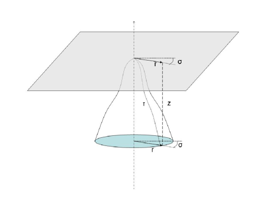
Figure 2: A curved surface with a central symmetry is embedded in a three-dimensional manifold. The reference frame is a plane and the global coordinates are cylindrical.

The $\tau$ coordinate is the radial coordinate in the natural manifold. The reference manifold is localized by means of the constraint $z=$ constant; the constraint for the natural frame is $z=f\left(r\right)$ being $f$ a non-linear function, otherwise one would have a cone, i.e. a flat sub-manifold. The global coordinates are $r,\sigma,z$; in the reference frame they are $r,\sigma$ coinciding with the first pair of global coordinates; in the natural frame the coordinates are $\tau$ and $\sigma$, with $\sigma$ coinciding with the corresponding global coordinate. Using the flatness of the embedding manifold we see that

$$d\tau^{2}=dr^{2}+dz^{2}=\left(1+f^{\prime 2}\right)dr^{2}$$ (15)

Of course $f^{\prime}$ is a shorthand notation for $df/dr$. If $f$ is a regular function (with the possible exception of the origin) from (15) we can work out $r\left(\tau\right)$.

It is easy to write down the distance between two nearby points on the reference frame directly adopting the appropriate signature:

$$ds^{2}=dr^{2}-r^{2}d\sigma^{2}+dz^{2}=dr^{2}-r^{2}d\sigma^{2}$$ (16)

The distance between the corresponding points in the natural frame is

$$ds^{\prime 2}=d\tau^{2}-r^{2}d\sigma^{2}=\left(1+f^{\prime 2}\right)dr^{2}-r^{2}d\sigma^{2}$$ (17)

We can read out the metric tensor on the curved manifold from (17 ), both in the $r,\sigma$ and the $\tau,\sigma$ coordinates, and, just to recover the formal correspondence with the RW notation, we may identify $r$ with $a\left(\tau\right)$.

The natural coordinates for our curved manifold are $\tau$ and $\sigma$, so, in order to proceed, we also need to cast (16) in terms of these coordinates; then:

$$ds^{2}=\frac{d\tau^{2}}{1+f^{\prime 2}}-a^{2}d\sigma^{2}$$ (18)

The difference between (17) and (18) is

$$ds^{\prime 2}-ds^{2}=f^{\prime 2}dr^{2}=\frac{f^{\prime 2}}{1+f^{\prime 2}}d\tau^{2}$$ (19)

Interpreting (19) on the light of sect. (2) we read out the only non-zero element of the strain tensor of the natural frame and using the coordinates thereupon (use (15))

$$\varepsilon_{\tau\tau}=\frac{f^{\prime 2}}{2\left(1+f^{\prime 2}\right)}=\frac{1-\dot{a}^{2}}{2}$$

With a little change in the notation we put $\dot{a}=dr/d\tau$; the reason is to conform to the standard notation for a RW universe.

4.1 $4+1$-dimensional embedding

The above treatment, when applied to the full four-dimensional manifold we use to describe the universe, actually corresponds to a negatively curved space (space curvature constant $k=-1$), as can be seen by noting that the choice $z=constant$ gives a flat Lorentzian manifold only if $d\sigma^{2}=d\chi^{2}+\sinh^{2}\chi\left(d\theta^{2}+\sin^{2}\theta d\phi^{2}\right)$, which corresponds to a three-dimensional negatively curved space. Of course we would like to analyze the null space curvature case since cosmological observations point in that direction. Let us then look a little more in detail to the geometry of our manifolds and to the meaning of the $\sigma$ variable we used in the previous section. Actually various embedding strategies have been adopted for similar purposes [59, 51]. We shall stay with our "cylindrical" symmetry approach and write a five-dimensional flat line element in the form:

$$ds_{5}^{2}=d\tau^{2}-d\sigma_{0}^{2}+dz^{2}$$ (20)

Here $d\sigma_{0}$ is the three-dimensional space line element in the null space curvature case:

$$d\sigma_{0}^{2}=dr^{2}+r^{2}\left(d\theta^{2}+\sin^{2}\theta d\phi^{2}\right);$$

$z$ is the fifth coordinate of the embedding space-time. With this coordinate choice, if we put $z=constant$ we recover a 4-dimensional flat sub-manifold, while RW symmetry with $k=0$ is obtained with the following transformation, as shown in [59, 51]:

$$\left\{\begin{array}[]{rl}r&\rightarrow a(\tau)\ r\\ \tau&\rightarrow\tau(r,\tau)\\ z&\rightarrow z(r,\tau),\end{array}\right.$$

Here $a(t)$ is the scale factor in the four-dimensional RW metric, and the explicit transformation for $\tau$ and $z$ are

$$dt = \left(\dot{a}+\frac{1}{\dot{a}}+\dot{a}r^{2}\right)d\tau/2+a(\tau)rdr$$

$$dz = \left(\dot{a}-\frac{1}{\dot{a}}-\dot{a}r^{2}\right)d\tau/2-a(\tau)rdr.$$

The final purpose is to work out the strain tensor that, using (13), turns out to only have spatial components:

$$\varepsilon_{\mu\nu}=\left\{\begin{array}[]{cll}0&if&\mu=\nu=1\\ \frac{1}{2}\left(1-a^{2}\right)&if&\mu=\nu=2,3,4\\ 0&if&\mu\neq\nu.\end{array}\right.$$

We can now compute the trace and the second order scalar that appear in the elastic Lagrangian (11):

$$\varepsilon_{\alpha\beta}g^{\alpha\beta}=\varepsilon=\frac{3}{2}\frac{\left(a^{2}-1\right)}{a^{2}}\quad\quad\varepsilon_{\alpha\beta}\varepsilon^{\alpha\beta}=\frac{1}{3}\varepsilon^{2}.$$

In the case of non-null spatial curvature the dependence of the strain tensor on the scale factor is different according to the sign of the curvature parameter. In practice the embedding strategy requires different coordinates and different transformations for each $k$ value. Recalling sec. (4), we see that the strain tensor both for positive and negative spatial curvatures has only one component different from zero, namely the time-time component:

$$\varepsilon_{\tau\tau}=\frac{1}{2}(1+k\dot{a}^{2}),\quad\quad k=\pm 1.$$

In the case of a negative space curvature this has been explicitly worked out in our 2+1-dimensional example. For the $k=1$ case, however, the reference four-dimensional flat manifold has to be Euclidean, even though the natural manifold has a Lorentzian signature. This is due to the fact that the 3-dimensional spatial sub-manifold is a 2-sphere.

4.2 The space-time behaviour

Let us now maintain a RW symmetry and study the case of an empty space-time in which space is also flat ($k=0$) as apparently it is for the actual universe. The action integral (12) becomes

$$S=\int\left[-6\left(a\ddot{a}+\dot{a}^{2}\right)a+L_{e}\right]d\tau,$$ (21)

with

$$L_{e}=\frac{1}{2}\left(\lambda+\frac{2}{3}\mu\right)\varepsilon^{2}\sqrt{\left|g\right|}=\frac{9}{8}B\frac{\left(1-a^{2}\right)^{2}}{a},$$

where $B=\lambda+\frac{2}{3}\mu$ is the bulk modulus of the continuum. Here we are using a point Lagrangian and we shall derive the equations of motion varying the action in eq.(21). We can remark that, in the absence of a defect, a RW space-time would in general not be a solution of the Lagrange equations obtained from (12): the symmetry (and the defect) are a priori conditions thus forcing the action integral (21).

Since second order derivatives in the Lagrangian appear linearly we can get rid of them by means of an integration by parts so that the effective Lagrangian density becomes

$$L=6a\dot{a}^{2}+L_{e}$$ (22)

We can work out the energy function, $W=\frac{\partial L}{\partial\dot{a}}\dot{a}-L$, which is, by construction, a conserved quantity:

$$W=6a\dot{a}^{2}-\frac{9}{8}B\frac{\left(1-a^{2}\right)^{2}}{a}.$$ (23)

Solving (23) for $\dot{a}$ we have

$$\dot{a}^{2}=\frac{W}{6a}+\frac{3}{16}B\frac{\left(1-a^{2}\right)^{2}}{a^{2}}$$ (24)

We see that for $a\rightarrow 0$ one has $\dot{a}\rightarrow\infty$. For $a\rightarrow\infty$ $\dot{a}$ diverges also.

The expansion rate in (24) has a minimum, which means that at the beginning the expansion is decelerated, then it becomes accelerated.
The trend of (24) appears in fig.(3) for arbitrary positive values of both parameters.
In order to recover General Relativity in the absence of defects, the energy function must be set to zero so that from now on we assume $W=0$.

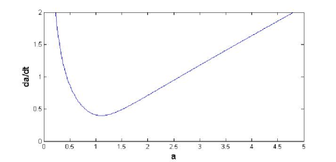
Figure 3: Expansion rate of a Robertson Walker space-time versus the scale factor, according to the theory. The space is assumed to be flat. Arbitrary positive values of the parameters have been used.

5 Expansion of the universe

The main fact we want to account for is the accelerated expansion of the universe, so in the present section we will deal with the data evidencing this phenomenon. We of course shall proceed according to our approach, but in the following we would also like to show how the same formulae can be read and interpreted in more traditional ways.

5.1
Dark fluid interpretation

Let us put together the first integral in (24) and the second order evolution equation, deduced from the point-Lagrangian in (22):

$$H^{2}= \frac{3}{16}B\frac{(a^{2}-1)^{2}}{a^{4}}$$ (25)

$$-2\ddot{a}a- \dot{a}^{2}= -\frac{3}{16}B\frac{(a^{2}-1)}{a^{2}}(3a^{2}+1),$$ (26)

$H$ is the Hubble parameter. Interpreting the r.h.s. of the equations as representing a fluid component, we may read out the corresponding density and pressure:

$$\rho = \frac{9}{16}B\frac{(a^{2}-1)^{2}}{a^{4}}$$ (27)

$$p = -\frac{3}{16}B\frac{(a^{2}-1)}{a^{4}}(3a^{2}+1)$$ (28)

The state parameter, i.e. $w=p/\rho$, would clearly depend on time. Since we are interested here in late cosmology, let us derive the condition for the acceleration to occur. An accelerating phase, $\ddot{a}>0$, requires $\rho+3p<0$. In our model it turns out to be

$$\rho+3p=-\frac{9B}{8}\frac{a^{4}-1}{a^{4}},$$ (29)

so acceleration sets in when $a^{4}>1$, or, in terms of the redshift $z=a_{0}/a-1$, when $z<a_{0}-1$. The parameter $a_{0}$ is the present scale factor and its value depends on the model and the observation.
In particular, if we write down the equation for the "elastic" state parameter

$$w=\frac{p}{\rho}=-\frac{1}{3}\frac{3a^{2}+1}{a^{2}-1}$$

we can easily see that the behaviour of the elastic potential tracks radiation, curvature and cosmological constant as $a$ increases, passing from $w=1/3$ in the $a\rightarrow 0$ limit to $w=-1$ for $a\rightarrow\infty$. In a 3+1 view we may think that, close to the cosmic defect, a release of "elastic" energy in form of radiation (primordial gravitational waves) dominates; afterwards this radiation is progressively converted into the equivalent of a "dark energy" driving an accelerated expansion, just as a cosmological constant would do.

5.2 Type Ia supernovae luminosity

The most direct evidence for the acceleration of the expansion comes from the luminosity data from the type Ia supernovae. In order to test the theory on the SnIa data we must include in our analysis the presence of matter. This will be done as usual introducing in the Lagrangian a matter term minimally coupled to geometry. It is

$$H^{2}=\frac{3}{16}B\frac{\left(1-a^{2}\right)^{2}}{a^{4}}+\kappa\sum\limits_{i}\rho_{i0}\frac{a_{0}^{3\left(1+w_{i}\right)}}{a^{3\left(1+w_{i}\right)}}$$ (30)

The coupling constant $\kappa$ is $16\pi G/c^{2}$ and $w_{i}$ is determined by the equation of state of the $i_{th}$ component; $\rho_{i0}$ is the mass/energy density of the $i_{th}$ component in the comoving frame, the index $0$ refers to present day values. The luminosity is commonly expressed in terms of the distance modulus and the redshift parameter appearing in the scale factor through $a=a_{0}/\left(1+z\right)$. It is [60]

$$m-M=25+5\log\left(\left(1+z\right)\int_{0}^{z}\frac{dz^{\prime}}{H(z^{\prime})}\right)$$ (31)

For (31) to hold, distances have to be measured in Mpc.

The simplest is to restrict to dust and radiation, for which $w$ is respectively $0$ and $1/3$; re-organizing the constants, the Hubble parameter is

$$H=\sqrt{\frac{B}{16}}\sqrt{3\left(1-\frac{(1+z)^{2}}{a_{0}^{2}}\right)^{2}+\frac{8\kappa}{3B}(1+z)^{3}\left[\rho_{m0}+\rho_{r0}(1+z)\right]}$$ (32)

Using (32), eq.(31) gives the explicit form of the distance modulus.

5.3 Fitting the data

Once (32) has been introduced into (31) we may use an optimization procedure in order to fit the luminosity data from type Ia supernovae. The implied range of values of $z$ ($\leq\sim 2$) is sufficiently small to assume that the radiation contribution is negligible ($\rho_{r0}\simeq 0$).

The distance modulus (31) can be written in terms of three optimization parameters and the new integration variable $\zeta=\left(1+z\right)/a_{0}$ , as in the following

$$m-M=\mathfrak{m}+5\log\left(\left(1+z\right)\int_{1/a_{0}}^{\zeta}\frac{d\zeta^{\prime}}{\sqrt{3\left(\zeta^{\prime 2}-1\right)^{2}+\psi\zeta^{\prime 3}}}\right)$$ (33)

where

$$\left\{\begin{array}[]{c}\mathfrak{m}=25+\frac{5}{2}\log 16-\frac{5}{2}\log B+5\log a_{0}\\ \psi=\frac{8\kappa\rho_{0}}{3B}a_{0}^{3}\end{array}\right.$$ (34)

We have compared the results in (33) with the data of 307 SnIa’s from the Supernova Cosmology Project union survey [61]. The best fit is shown on fig.4.

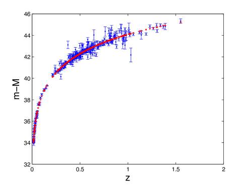
Figure 4: Fit of the luminosity data from 307 type Ia supernovae obtained applying the CD theory. Three optimization parameters have been used. The reduced $\chi^{2}$ of the fit is $1.017$.

The optimal parameters values are:

$$\left\{\begin{array}[]{c}\mathfrak{m}=46\pm 1\\ a_{0}=1.97\pm 0.04\\ \psi=10.1\pm 0.3\end{array}\right.$$ (35)

Considering the different sensitivity with respect to changes in $\mathfrak{m}$, which is outside the logarithm in (33), and in $a_{0}$ and $\psi$ , which are in the logarithm, the optimization has been performed in two steps. In the first step the optimization routine [62] has been run with all three parameters giving the actual value for $\mathfrak{m}$ and a first estimate of $a_{0}$ and $\psi$ (actually $1.98$ and $10.18$) with a big uncertainty (up to $100\%$ in the case of $\psi$). In the second step $\mathfrak{m}$ has been fixed to its already found value and the routine has been used again with the two remaining free parameters, thus yielding a far better uncertainty. The final reduced $\chi^{2}$ of the fit is $1.017$.

We compare our result with what can be obtained using the $\Lambda CDM$ theory. In this case the distance modulus, expressed in terms of two free parameters, is [48]

$$m-M=\mu+5\log\left(1+z\right)+5\log\int_{0}^{z}\frac{dz^{\prime}}{\sqrt{\Omega_{m}\left(1+z^{\prime}\right)^{3}+1-\Omega_{m}}}$$ (36)

Using the same two-steps optimization process the final $\chi^{2}$ is $1.019$, so we see that the $CD$ fit is better.

Let us now deduce some cosmological parameters from our best fit values by using (34) and (35). Eliminating $B$ between the first and the second equation of (34) we find a relation among all parameters we have used for the fit, and $\rho_{0}$:

$$\mathfrak{m}=25+\frac{5}{2}\log\frac{6\psi}{\kappa\rho_{0}a_{0}}.$$ (37)

The actual value of the mass/energy density in the universe is not easy to assess, but is usually thought to be somewhere between $10^{-27}$ and $10^{-28}$ kg/m³.
By using eq.(37) we can derive the estimated mass density from our fit, and it is $\rho_{0}\sim 3.4\times 10^{-27}kg/m^{3}$. This is but a rough estimate because the SnIa data do not allow for more accurate results. Actually the uncertainty domain for $\rho_{0}$ is in the order of $100\%$. Another estimate we can do concerns the value of the Hubble constant $H_{0}$. From (32), neglecting the contribution from radiation, we have:

$$H_{0}=c\sqrt{\kappa\rho_{0}}\sqrt{\frac{1}{2\psi}\frac{\left(1-a_{0}^{2}\right)^{2}}{a_{0}}+\frac{1}{6}}$$ (38)

Introducing the numerical values we found for the parameters, we have

$$H_{0}=64\pm 35\ \frac{km}{s\times Mpc}.$$

Once more the big uncertainty comes mainly from the uncertainties in the luminosity data of SnIa’s.

Until now we have avoided the explicit use of the $B$ parameter, however this parameter, in our theory, has the simple physical meaning of bulk modulus of space-time, so let us compute it. From the first equation of the (34) we obtain:

$$B=\left(3\pm 2\right)\times 10^{-7}Mpc^{-2}=\left(3\pm 2\right)\times 10^{-52}m^{-2}.$$ (39)

Looking back at equation (24) we find for B the constraint $B>0$, which is indeed satisfied by (39).

6 Newtonian limit of the theory

After having found a good correspondence between theory and data at the level of the SnIa luminosity dependence on redshift we should also verify that a correct weak energy (Newtonian) limit exists. To that purpose we start with some general remarks. Since in practice our theory simply additively introduces a peculiar source term into the Lagrangian of space time, whenever this new term is sent to zero we of course recover plain GR with all its features and local limits. It would not be so only if the additional term (11) were somehow singular, which is not the case. In fact, excluding the very cosmic defect, $L_{e}$ can continuously go to zero at any place, together with the local strain.

We think this could be enough, however let us explicitly verify what the weak field limit is. In order to make this check, let us consider a spherically symmetric, stationary physical system. We know that the general line element for this problem is

$$ds^{2}=f\left(r\right)d\tau^{2}-h\left(r\right)dr^{2}-r^{2}d\theta^{2}-r^{2}\sin^{2}\theta d\varphi^{2}$$ (40)

where Schwarzschild coordinates are used.

It is easy to read our strain tensor (its non-zero elements) out of the metric in (40) comparing it with a Minkowski line element in spherical coordinates. We get:

$$\begin{array}[]{cc}\varepsilon_{00}&=\frac{f-1}{2}\\ \varepsilon_{rr}&=\frac{1-h}{2}\end{array}$$ (41)

Equipped with (41) we are able to explicitly work out (11) for our problem, then we write the corresponding Lagrangian for empty space-time (no matter, except at the source of the local spherical symmetry). Modulo an unessential $\sin\theta$ factor and after eliminating a second order derivative of $f$ by a by part integration, the explicit formula is (primes mean derivatives with respect to $r$):

$$\begin{array}[]{cc}L&=-\frac{2fh^{\prime}r+2fh^{2}-2fh}{h\sqrt{fh}}+\frac{\lambda}{4}\frac{\left(f-1\right)\left(h-1\right)}{\sqrt{fh}}r^{2}\\ &+\frac{1}{4}\left(\mu+\frac{\lambda}{2}\right)\left(\frac{\left(f-1\right)^{2}}{f^{2}}+\frac{\left(h-1\right)^{2}}{h^{2}}\right)\sqrt{fh}r^{2}\end{array}$$ (42)

From (42) we obtain the Euler-Lagrange equations for $f$ and $h$:

$$fh-rf^{\prime}-f = \frac{r^{2}}{16fh}\left\{\lambda\left[\left(\left(2h+1\right)^{2}-5\right)f^{2}-4fh^{2}+\left(f-h\right)^{2}\right]\right..$$ (43)

$$\left.+2\mu\left[\left(2h^{2}+2h-3\right)f^{2}+\left(1-2f\right)h^{2}\right]\right\}$$

$$rh^{\prime}+h^{2}-h = \frac{r^{2}}{16f^{2}}\left\{\lambda\left[\left(4f-3\right)h^{2}+\left(2h-1\right)^{2}f^{2}-2fh\right]\right.$$ (44)

$$\left.+2\mu\left[\left(2f+f^{2}-3\right)h^{2}+f^{2}\left(1-h\right)^{2}\right]\right\}$$

The left hand side of eq.s (43-44) corresponds to the equations for the Schwarzschild problem, whilst the right hand side can be considered to be "small" as far as it is

$$r^{2}\mu,r^{2}\lambda<<1$$ (45)

Under the latter assumption we may look for solutions like:

$$\left\{\begin{array}[]{c}f=f_{0}+f_{1}\\ h=h_{0}+h_{1}\end{array}\right.$$ (46)

where

$$\left\{\begin{array}[]{c}f_{0}=1-2\frac{m}{r}\\ h_{0}=\frac{1}{f_{0}}\end{array}\right.$$

is the Schwarzschild solution ($m=GM/c^{2}$) and

$$f_{1},h_{1}\sim\lambda,\mu$$ (47)

Under the ansatz (46) and condition (47) eq.s (43-44) may be solved to first order in $\lambda$, $\mu$. The result is:

$$\left\{\begin{array}[]{c}f_{1}=\frac{C}{r}+\left(3m^{2}\mu-A\right)\left(1-2\frac{m}{r}\right)+\lambda\left(\frac{6m^{3}+4m^{3}\ln\left(r-2m\right)}{r}-\frac{m^{4}}{r^{2}\left(1-2\frac{m}{r}\right)}\right)\\ +\mu\left(\frac{20m^{3}}{r}-\frac{2m^{4}}{r^{2}\left(1-2\frac{m}{r}\right)}+\left(\allowbreak 22\frac{m^{3}}{r}-6m^{2}\right)\ln\left(r-2m\right)-\frac{3}{2}mr\left(1-2\frac{m}{r}\right)\right)\\ h_{1}=\frac{C}{r\left(1-2\frac{m}{r}\right)^{2}}+\frac{\lambda}{r\left(1-2\frac{m}{r}\right)^{2}}\left(\frac{3m^{4}}{r\left(1-2\frac{m}{r}\right)}-m^{2}r-4m^{3}\ln\left(r-2m\right)\right)\\ +\frac{\mu}{r\left(1-2\frac{m}{r}\right)^{2}}\left(\frac{6m^{4}}{r\left(1-2\frac{m}{r}\right)}-3m^{2}r-\frac{m}{2}r^{2}-10m^{3}\ln\left(r-2m\right)\right)\end{array}\right.$$ (48)

Here $A$ and $C$ are integration constants. $A$ is used to remove constant contributions from $f_{1}$.

Up to this moment we have not used the assumption that the gravitational field is weak. Let us introduce this condition now, linearizing the results in $m/r$. The result is

$$\left\{\begin{array}[]{c}f_{1}\simeq\frac{C}{r}-\frac{3}{2}\mu mr\\ h_{1}\simeq\frac{C}{r}+4\frac{Cm}{r^{2}}-\frac{1}{2}\mu mr\end{array}\right.$$

As for the integration constant $C$, it contributes a redefinition of the mass of the spherical source and a short range contribution to $h_{1}$; fixing $C=0$ we finally have:

$$\left\{\begin{array}[]{c}f=1-2\frac{m}{r}-\frac{3}{2}\mu mr\\ h=1+2\frac{m}{r}-\frac{1}{2}\mu mr\end{array}\right.$$ (49)

The solutions (49) are acceptable, as already said, as far as condition (45) holds. Now condition (45) can be updated to

$$r<<\frac{1}{m\mu}$$

If we consider the example of a Sun-like star, where it is $m\sim 10^{3}$ m, and use the result found for $B$ in the previous section (reasonably it is also $\mu\sim B$) we obtain

$$r<<10^{49}m\sim 10^{27}Mpc\sim 10^{33}lightyears$$

As we see all deviations of our theory from the standard GR, at the Solar System or galaxy clusters level, are absolutely negligible. The only effect is at the cosmic level.

7 Conclusion

We have exploited the existing analogy between the theory of elasticity and GR and this approach has given good fruits, however, recalling the open questions we posed in the Introduction, we remark here that an analogy is not an identity; we are not allowed to mechanically transpose one theory on top of the other. In GR one properly looks for "static" solutions in four dimensions: various possible configurations of the full four-dimensional universe are studied, but there is no evolution because there is no evolution parameter out of the manifold. Time is part of the manifold and the dynamic term in the Lagrangian is the scalar curvature which contains second order derivatives of the Lagrangian coordinates, i.e. of the elements of the metric tensor, with respect to an arbitrary set of Gaussian coordinates. In the case of elasticity the three-dimensional manifold has Euclidean signature and time is the absolute Newtonian time; the dynamics is expressed by time derivatives. The difference is paramount.

The role of the defect(s) in our theory deserves also some additional comments. There are indeed, in the three-dimensional theory of continua, situations where one has to do with continuous distributions of (micro)defects, rather than with localized defects. This happens mainly as a consequence of a plastic deformation: an initial stress in the material is eased (for instance by reheating) and produces a distributed defects field. The final result of this process is indeed the disappearance of the internal strain and a permanent plastic deformation of the manifold. This situation does not correspond to what we want to describe, since for us the strain represents the gravitational field, or the non-trivial part of the metric tensor, and we want it to stay there and disappear only when its causes are removed (no plastic shear). This is the reason why our attention is focused on a localized defect responsible for a global spontaneous strain state and for the related symmetry. An appealing possibility could be to have a plurality of localized defects which would give rise to some more complicated strain pattern; one could be tempted to identify these defects with matter. We have not dared, for the moment, to pursue this idea, so in our theory, at present, matter is treated as usually it is, appearing in the Lagrangian as an additional independent term coupled with the (strained) geometry via the metric tensor.

In the above conceptual background we have combined the classical GR approach with the description of space-time by means of the linear theory of elasticity, preserving general covariance and all the features of GR. The expansion of the universe is consequently described in terms of a strained four-dimensional continuum (space-time), whose strain has partly an intrinsic origin due to the presence of a cosmic defect, partly depends on extrinsic sources, i.e. matter fields. The cosmic defect fixes the global symmetry of the universe, then the general features of what, in our ($3+1$)-split view, is the cosmic expansion. This approach can be applied to any kind of universe with any global symmetry depending on the possible defects, just as it happens in three dimensional solid materials. We have then assumed the basic "stuff", i.e. space-time, to be locally homogeneous and isotropic, as a consequence of the global homogeneity and isotropy of the flat unstrained reference manifold and of the linearity of the theory. Working out the global configuration of space-time for a RW symmetry (the typical symmetry assumed to hold, on a cosmic scale, for our universe) we have found that it naturally includes an initial extremely rapid expansion with a steeply decreasing expansion rate, followed by acceleration. We have also verified that the inclusion of matter in the form of fluid(s) preserving the global symmetry does not modify the general structure of the expansion. The theory depends on three parameters, which are the present scale factor of the universe $a_{0}$, the bulk modulus of space-time $B$, and the present day matter/energy density of the universe $\rho_{0}$. Using these three quantities as optimization parameters we have fitted the luminosity data of type Ia supernovae. The result has been good, and the value obtained for $\rho_{0}$ is consistent with the current estimates for barionic matter without a need for more matter, but the uncertainty due to the accuracy of the luminosity data is very high. According to the theory no further dark energy is needed; however, if we wish, we may read our elastic contribution as a dark energy fluid, whose density and pressure have been explicitly written, it would however be rather difficult to find a reasonable physical interpretation for the properties of this peculiar fluid.

A final remark concerns the signature of our manifolds. It always is Lorentzian in the natural manifold which we want to represent the actual universe. As for the reference manifold it can either be Euclidean or Minkowskian and the embedding strategy can easily produce one or the other of them. It is sufficient to assume the embedding flat higher dimensional manifold to be Minkowskian. Whenever then the reference submanifold is a space-like hyperplane (time-like normal vector) its geometry is naturally Euclidean; viceversa, choosing as a reference submanifold a time-like hyperplane, it will turn out to be Minkowskian.

Although the theory has been applied to the cosmic scale, we have also verified that it has a correct Newtonian limit and, with the value of the parameters obtained from the SnIa’s fit, it is indistinguishable from GR at the Solar system as well as at the galaxy clusters scale.

References

References

- [1] Perlmutter S et al 1999 Astrophys. J. 517 565–586
- [2] Riess A G et al. 1998 Astron. J. 116 1009–1038
- [3] De Bernardis P et al 200 Nature 404 955–959
- [4] Hanany S et al. 2000 Astrophys. J. 545 L5.
- [5] Spergel D N 2007 et al. 2007 Astrophys. J. Suppl. 170 377–408
- [6] Zwicky F 1933 Helv. Phys. Acta 6 110–127
- [7] Zwicky F 1937 Astrophys. J. 86 217
- [8] Stanek R. et al. 2006 Astrophys. J. 648 956–968
- [9] Tegmark M et al. 2003 Astrophys. J.606 702–740
- [10] Guth A.H. Phys. Rev.D 1981 23 347–356
- [11] Linde A D 1982 Phys. Lett.B 108 389–393
- [12] Lemoine M, Martin J and Peter P 2008 Inflationary cosmology, volume 738 of Lect. Notes Phys., Springer, Heidelberg
- [13] Linde A D 1994Phys. Rev.D 49 748
- [14] Cai Y F, Li H, Piao Y S and Zhang X2007 Phys. Lett.B 646 141–144
- [15] Armendáriz-Picon C, Damour T and Mukhanov V 1999 Phys. Lett.B 458 209–218
- [16] Garriga J and Mukhanov V 1999 Phys. Lett.B 458 219–225
- [17] Golovnev A, Mukhanov V and Vanchurin V 2008 JCAP 06 009
- [18] Einstein A 1917 Konigl. Preuss. Akad. Wiss. 142–152
- [19] Einstein A 1931 Sitz. der Preuss. Akad.Wiss. 235–237
- [20] Sahni V and Starobinski A 2000 Int. J. Mod. Phys. D. 9 373–443
-
[21]
Carroll S M 2001 Living Rev. Rel. 4
1 Cited on July 2009.
Online article: http://relativity.livingreviews.org/Articles/lrr-2004-4. - [22] Zlatev I, Wang L and Steinhardt P J 1999 Phys. Rev. Lett.82 896–899
- [23] Carroll S M 1998 Phys. Rev. Lett.81 3067
- [24] Caldwell R R 2002 Phys. Lett.B 545 23–29
- [25] Vikman A 2005 Phys. Rev.D 71 023515
- [26] Zhang X and Wu F Q 2005 Phys. Rev.D 72043524
- [27] Li M 2004 Phys. Lett.B 603 1
- [28] Pavon D and Zimdahl W 2005Phys. Lett.B 628 206–210
- [29] Armendariz-Picon C 2004 JCAP 07 007
- [30] Armendariz-Picon C, Mukhanov V and Steinhardt P J 2000 Phys. Rev. Lett.85 4438
- [31] Del Popolo A 2007 Astron. Rep. 51169–196
- [32] Hannestad S, Mirizzi A, Raffelt G C and Wong. Y Y Y 2008 JCAP 04 019
- [33] Dubovsky S L, TInyakov P G and Tkachev. I I 2005 Phys. Rev. Lett.94 181102
- [34] Palazzo A, Cumbercatch D, Slosar A and Silk 2007 Phys. Rev.D 76 013511
- [35] Hinshaw G et al. 2009 Astrophys. J. Suppl. 180 225–245
- [36] Capozziello S and Francaviglia M 2008 Gen.Rel. Grav. 40 357–420
- [37] Sotiriou T and Faraoni V 2008 o appear on Rev. Mod. Phys.http://arxiv.org/abs/0805.1726
- [38] Milgrom M 1983 Astrophys.J. 270 365–370
- [39] Milgrom M 1983 Astrophys.J. 270 371–383
- [40] Milgrom M 1983 Astrophys.J. 270 384–389
- [41] Bekenstein J D 2004 Phys. Rev.D 70
- [42] Mavromatos N E2002 Lect. Notes Phys.592 392–457
-
[43]
Maartens R 2004 Living Rev. Rel. 7
7 Cited on July 2009.
Online article: http://www.livingreviews.org/lrr-2004-7. - [44] Bojowald M 2001 Phys. Rev. Lett.86 5227
-
[45]
Bojowald M 2008 Living Rev. Rel. 11
4, Cited on March 2009.
Online article: http://relativity.livingreviews.org/Articles/lrr-2008-4. -
[46]
Einstein A 2007 In The Collected Papers of
Albert Einstein, volume 7. Princeton University Press, Princeton, 2007.
Archives Online, http://alberteinstein.org/, Call. Nr.[1-41.00]. - [47] Tartaglia A and Capone M 2008 Int. J. Mod. Phys. D 17 275–299
- [48] Tartaglia A Capone M Cardone V and Radicella N 2008 Int. J. Mod. Phys. D 19 1453
- [49] Landau L and Lifshitz E 1986 Theory of elasticity. Pergamon Press, Oxford, third edition
- [50] Eshelby J D 1956 Solid state physics Academy Press, New York, 1956.
- [51] Rosen J 1965 Rev. Mod. Phys.37 204–214
- [52] Sachs R K 1964 In Relativity, Groups and Topology. Gordon and Breach, New York
- [53] Valsakumar M C and Sahoo D 1988 Bull. Mater. Sci. 10 3–44
- [54] Volterra V 1904 Ann. Sci. de l’ É.N.S. 24 401–517
- [55] Puntigam R A and Soleng H H 1997 Class. Quantum Grav.14 1129–1149
- [56] Nabarro F R 1979 Dislocations in solids. North Holland, Amsterdam
- [57] Hirth J P and Lothe J 1982 Theory of dislocations. John Wiley and Sons, New York, second edition
- [58] Hawking S and Ellis GFR 1973 The Large Scale Structure of Space-Time. Cambridge University Press, Cambridge
- [59] Lachieze-Rey M 2000 Astronomy and Astrophysics 364 894–900
- [60] Weinberg. 1972Gravitation and Cosmology: Principles and Applications of the general theory of Relativity John Wiley and Sons, New York,
- [61] Kowalski M et al. Astrophys. J. 686 749–778
- [62] Allodi. http://www.fis.unipr.it/giuseppe.allodi/Fminuit/ Fminuit-download.html.