A numerical investigation of the steady states
of the spherically symmetric Einstein-Vlasov-Maxwell system

Abstract

We construct, by numerical means, static solutions of the spherically symmetric Einstein-Vlasov-Maxwell system and investigate various features of the solutions. This extends a previous investigation [5] of the chargeless case. We study the possible shapes of the energy density profile as a function of the area radius when the electric charge of an individual particle is varied as a parameter. We find profiles which are multi-peaked, where the peaks are separated either by vacuum or a thin atmosphere, and we find that for a sufficiently large charge parameter there are no physically meaningful solutions. Furthermore, we investigate if the inequality

$$\sqrt{M}\leq\frac{\sqrt{R}}{3}+\sqrt{\frac{R}{9}+\frac{Q^{2}}{3R}},$$

derived in [2], is sharp within the class of solutions to the Einstein-Vlasov-Maxwell system. Here $M$ is the ADM mass, $Q$ the charge, and $R$ the area radius of the boundary of the static object. We find two classes of solutions with this property, while there is only one in the chargeless case. In particular we find numerical evidence for the existence of arbitrarily thin shell solutions to the Einstein-Vlasov-Maxwell system. Finally, we consider one parameter families of steady states, and we find spirals in the mass-radius diagram for all examples of the microscopic equation of state which we consider.

1 Introduction

In this work matter is described as a large ensemble of charged particles which interact via the gravitational and electromagnetic fields created by the particles themselves. All the particles have the same rest mass, normalized to $1$, and the same charge $q_{0}\geq 0$. The distribution of the particles on phase space is given by a density function $f$. The particle ensemble is assumed to be collisionless which implies that $f$ satisfies the Vlasov equation. Macroscopic quantities such as mass-energy density, pressure, and charge current, which act as source terms in the field equations, are obtained by integrating $f$ with respect to specific weight functions. The resulting system is called the Einstein-Vlasov-Maxwell system and is stated in Section 2. In the present work we construct, by numerical means, static solutions of the asymptotically flat, spherically symmetric Einstein-Vlasov-Maxwell system, and we investigate three different features of the solutions. In the chargeless case, i.e., for the spherically symmetric Einstein-Vlasov system, a similar study has been carried out in [5]. There is an essential difference between these two systems concerning known mathematical results of existence of static solutions and their properties. In the chargeless case it is known that a wide variety of static solutions with finite extent and finite ADM mass exist, cf. [4, 14], and the references therein, whereas the problem of existence of static solutions in the charged case has not yet been studied. The mathematical construction of steady states in the chargeless case is based on a certain ansatz for the density function $f.$ Here this ansatz is modified to handle the charged situation, cf. Section 3. We believe that this constitutes a natural starting point for showing existence of static solutions of the Einstein-Vlasov-Maxwell system, but we do not include such an analysis here since the purpose of the present paper is to investigate numerically three features of static solutions which we now describe in some detail.

In Section 4 an analysis of the behavior of the energy density as a function of area radius is carried out for different values of the charge parameter $q_{0}$. Qualitatively we find a similar structure as in the chargeless case [5], e.g. there are solutions with an arbitrary number of peaks, and these peaks are separated either by vacuum or by a thin atmosphere. The choice of charge parameter affects in some cases the number of peaks. If the charge parameter reaches a certain critical value the solutions break down before the energy density vanishes. It is natural to compare this with the Newtonian Vlasov-Poisson system for which there is no difference in the form of the equations whether one models a mono-charged plasma or a gravitating system, except for the sign in front of the force field. If one studies a charged gravitating system this sign is positive or negative depending on whether $q_{0}<1$ or $q_{0}>1$. Steady states with finite extent only exists in the former case where the effective force field is attractive. This is in accordance with what we find in the relativistic situation.

In Section 5 we investigate if there are static solutions of the Einstein-Vlasov-Maxwell system such that the inequality

$$\sqrt{M}\leq\frac{\sqrt{R}}{3}+\sqrt{\frac{R}{9}+\frac{Q^{2}}{3R}},$$ (1.1)

which was derived in [2], can be saturated in the sense that the quotient of the left and right hand side in (1.1) is arbitrarily close to one. If there are such solutions we say that the inequality (1.1) is sharp within this class of solutions. Here $M$ is the ADM mass, $Q$ the total charge, and $R$ the area radius of the boundary of the static object. It was shown in [2] that (1.1) holds for any static solution of the Einstein-Maxwell-matter system which satisfies the energy condition

$$p+p_{T}\leq\rho,$$ (1.2)

where $p\geq 0$ and $p_{T}\geq 0$ are the radial and tangential pressures respectively and $\rho\geq 0$ is the energy density. This condition is satisfied by Vlasov matter. A suitable extension of the inequality (1.1) also holds inside the static object, cf. [2] and Section 5. Moreover, it was shown in [2] that the inequality is sharp, and in particular that equality is attained by infinitely thin shell solutions. The method of proof in [2] is quite general and applies to any matter model for which (1.2) holds. However, the solution constructed in the analysis leading to sharpness has features which solutions of the Einstein-Vlasov-Maxwell system do not have. Hence, one motivation for the present study is to investigate if sharpness of the inequality can be attained by solutions when a real matter model is chosen so that the system of equations includes a matter field equation, in the case at hand the Vlasov equation. In contrast to the chargeless case it is not known if there are solutions other than infinitely thin shells which saturate (1.1), and it is not known if arbitrarily thin shell solutions do exist for the Einstein-Vlasov-Maxwell system.

In the uncharged case more is known. It follows from [3] that infinitely thin shell solutions are unique in saturating the inequality (1.1) for $Q=0$, i.e., the inequality

$$M\leq\frac{4R}{9}.$$

Since an infinitely thin shell solution is not a regular solution of the Einstein-matter system this statement should be interpreted in the sense that a sequence of regular solutions tending to an infinitely thin shell will in the limit give equality. Moreover, it is known [4] that regular arbitrarily thin shell solutions of the Einstein-Vlasov system do exist, which then in particular implies that there are steady states to this system such that $M/R$ is arbitrarily close to $4/9.$

In the present work we find numerical evidence for answering the issues raised above. Indeed, we construct arbitrarily thin shell solutions to the Einstein-Vlasov-Maxwell system, which saturate the inequality (1.1) in the limit. Moreover, in contrast to the uncharged case we also find another type of solutions which saturate the inequality. These solutions have the feature that $M,Q$, and $R$ are all equal; they represent an extremal object. The latter property may be of interest in fundamental black hole physics, cf. [6, 10, 9].

In Section 6 the third and final property is investigated, namely the relation between the ADM mass and the outer area radius of a one parameter family of steady states to the Einstein-Vlasov-Maxwell system. The one parameter family is obtained by prescribing the way in which $f$ depends on the local energy and the angular momentum, which we call the microscopic equation of state. We find numerical support for mass-radius spirals for all examples of the microscopic equation of state which we investigate. This agrees with the result in [5] in the chargeless case, but on the other hand it differs from the Newtonian situation where the presence of such spirals heavily depends on the microscopic equation of state. In [11, 13] the question of which equations of state in the fluid case give rise to spirals is investigated.

To conclude this introduction we mention [6, 8, 10] where numerical investigations of solutions to the Einstein-Maxwell system are carried out using other conditions on the matter model. These studies focus on the issue of bounding $M$ in terms of $Q$ and $R.$

2 The spherically symmetric Einstein-Maxwell-Vlasov system

We choose general local coordinates $x^{\alpha}$ on the spacetime manifold and we denote by $p^{\alpha}$ the corresponding canonical momenta; Greek indices always run from $0$ to $3$ and Latin ones from $1$ to $3$. We assume that $x^{0}=t$ is a timelike coordinate and that $p^{0}$ can be expressed by $p^{i}$ through the condition that all the particles have rest mass normalized to $1$: $g_{\alpha\beta}p^{\alpha}p^{\beta}=-1$. Then the Einstein-Vlasov-Maxwell system takes the following form:

$$F^{\leavevmode{\alpha\beta}\mathchoice{\makebox[7.589pt][c]{$\displaystyle$}}{\makebox[7.589pt][c]{$\textstyle$}}{\makebox[4.49565pt][c]{$\scriptstyle$}}{\makebox[3.21117pt][c]{$\scriptscriptstyle$}}}_{\mathchoice{\makebox[8.43729pt][c]{$\displaystyle$}}{\makebox[8.43729pt][c]{$\textstyle$}}{\makebox[5.9061pt][c]{$\scriptstyle$}}{\makebox[4.21864pt][c]{$\scriptscriptstyle$}}\leavevmode{;\alpha}}=4\pi\,J^{\beta},$$ (2.1)

$$F^{\mathchoice{\makebox[15.1725pt][c]{$\displaystyle$}}{\makebox[15.1725pt][c]{$\textstyle$}}{\makebox[9.80408pt][c]{$\scriptstyle$}}{\makebox[7.00291pt][c]{$\scriptscriptstyle$}}}_{\leavevmode{\beta\gamma;\alpha}}+F^{\mathchoice{\makebox[15.1725pt][c]{$\displaystyle$}}{\makebox[15.1725pt][c]{$\textstyle$}}{\makebox[9.80408pt][c]{$\scriptstyle$}}{\makebox[7.00291pt][c]{$\scriptscriptstyle$}}}_{\leavevmode{\gamma\alpha;\beta}}+F^{\mathchoice{\makebox[15.1725pt][c]{$\displaystyle$}}{\makebox[15.1725pt][c]{$\textstyle$}}{\makebox[9.80408pt][c]{$\scriptstyle$}}{\makebox[7.00291pt][c]{$\scriptscriptstyle$}}}_{\leavevmode{\alpha\beta;\gamma}}=0,$$ (2.2)

$$R_{\alpha\beta}-\dfrac{1}{2}g_{\alpha\beta}R=8\pi(T_{\alpha\beta}+\tau_{\alpha\beta}),$$ (2.3)

$$\partial_{t}f+\dfrac{p^{i}}{p^{0}}\partial_{x^{i}}f-\dfrac{1}{p^{0}}(\Gamma_{\alpha\beta}^{i}p^{\alpha}p^{\beta}+q_{0}p^{\alpha}F^{\mathchoice{\makebox[4.4779pt][c]{$\displaystyle$}}{\makebox[4.4779pt][c]{$\textstyle$}}{\makebox[3.13454pt][c]{$\scriptstyle$}}{\makebox[2.23895pt][c]{$\scriptscriptstyle$}}\leavevmode{i}}_{\leavevmode{\alpha}\mathchoice{\makebox[2.41159pt][c]{$\displaystyle$}}{\makebox[2.41159pt][c]{$\textstyle$}}{\makebox[1.68811pt][c]{$\scriptstyle$}}{\makebox[1.2058pt][c]{$\scriptscriptstyle$}}})\partial_{p^{i}}f=0,$$ (2.4)

where

$$T_{\alpha\beta}=-\int_{\mathbb{R}^{3}}p_{\alpha}p_{\beta}\sqrt{|g|}\dfrac{d^{3}p}{p_{0}},$$ (2.5)

$$\tau_{\alpha\beta}=\frac{1}{4\pi}\left(F^{\mathchoice{\makebox[4.4779pt][c]{$\displaystyle$}}{\makebox[4.4779pt][c]{$\textstyle$}}{\makebox[3.13454pt][c]{$\scriptstyle$}}{\makebox[2.23895pt][c]{$\scriptscriptstyle$}}\leavevmode{\gamma}}_{\leavevmode{\alpha}\mathchoice{\makebox[3.62411pt][c]{$\displaystyle$}}{\makebox[3.62411pt][c]{$\textstyle$}}{\makebox[2.53687pt][c]{$\scriptstyle$}}{\makebox[1.81206pt][c]{$\scriptscriptstyle$}}}F_{\beta\gamma}-\dfrac{g_{\alpha\beta}}{4}F_{\gamma\nu}F^{\gamma\nu}\right),$$ (2.6)

$$J^{\beta}=q_{0}\int_{\mathbb{R}^{3}}p^{\beta}f\sqrt{|g|}\dfrac{d^{3}p}{p_{0}}.$$ (2.7)

Here (2.1) and (2.2) are the Maxwell equations, (2.3) are the Einstein equations, (2.4) is the Vlasov equation, and $F_{;\alpha}$ denotes the covariant derivative.

We consider this system under the assumption of spherical symmetry. Hence the metric, expressed in Schwarzschild coordinates, takes the form

$$ds^{2}=-e^{2\mu(t,r)}dt^{2}+e^{2\lambda(t,r)}dr^{2}+r^{2}(d\theta^{2}+\sin^{2}\theta d\varphi^{2}),$$ (2.8)

where

$$t\geq 0,\ r\geq 0,\ \theta\in[0,\pi],\ \varphi\in[0,2\pi].$$ (2.9)

For the metric to approach that of Minkowski space as $r$ goes to infinity, the boundary conditions

$$\lim_{r\to\infty}\lambda(t,r)=\lim_{r\to\infty}\mu(t,r)=0$$ (2.10)

are imposed. Furthermore, the condition

$$\lambda(t,0)=0$$ (2.11)

ensures a regular center. We introduce the corresponding Cartesian coordinates $x=(x^{1},x^{2},x^{3})=r(\sin\theta\cos\varphi,\sin\theta\sin\varphi,\cos\theta)$ and find that

$$p_{0}=-e^{\mu}\sqrt{1+|p|^{2}+(e^{2\lambda}-1)\left(\frac{x\cdot p}{r}\right)^{2}}.$$

Here $x\cdot p$ denotes the Euclidean scalar product of the vectors $x=(x^{1},x^{2},x^{3}),\ p=(p^{1},p^{2},p^{3})$, and $|\cdot|$ denotes the Euclidean norm on $\mathbb{R}^{3}$. For a spherically symmetric electric field of the form

$$E^{i}=\varepsilon\dfrac{x^{i}}{r}$$

the non-zero components of the electromagnetic field-strength tensor are

$$F^{0i}=e^{-\mu}\varepsilon\dfrac{x^{i}}{r}.$$

Let

$$w=\frac{x\cdot v}{r},\qquad L=|x\times v|^{2}=r^{2}(|v|^{2}-w^{2}),$$

where

$$v^{i}=p^{i}+(e^{\lambda}-1)\dfrac{x\cdot p}{r}\dfrac{x^{i}}{r};$$

the variables $w$ and $L$ can be viewed as the momentum in the radial direction and the square of the angular momentum, respectively, expressed in a suitable frame. The system now reads

$$q^{\prime}=4\pi r^{2}\rho_{q},$$ (2.12)

$$e^{-2\lambda}(2r\lambda^{\prime}-1)+1=8\pi r^{2}\rho+\dfrac{q^{2}}{r^{2}},$$ (2.13)

$$e^{-2\lambda}(2r\mu^{\prime}+1)-1=8\pi r^{2}p-\dfrac{q^{2}}{r^{2}},$$ (2.14)

$$\partial_{t}f+e^{\mu-\lambda}\dfrac{w}{\sqrt{1+w^{2}+L/r^{2}}}\partial_{r}f-\biggl{(}e^{\mu-\lambda}\mu^{\prime}\sqrt{1+w^{2}+L/r^{2}}+\dot{\lambda}w$$

$$\qquad\qquad\qquad-e^{\mu}\dfrac{q_{0}q}{r^{2}}-e^{\mu-\lambda}\dfrac{L}{r^{3}\sqrt{1+w^{2}+L/r^{2}}}\biggr{)}\partial_{w}f=0,$$ (2.15)

where

$$\rho=\dfrac{\pi}{r^{2}}\int_{-\infty}^{\infty}\int_{0}^{\infty}\sqrt{1+w^{2}+L/r^{2}}\,f\,dL\,dw,$$ (2.16)

$$p=\dfrac{\pi}{r^{2}}\int_{-\infty}^{\infty}\int_{0}^{\infty}\dfrac{w^{2}}{\sqrt{1+w^{2}+L/r^{2}}}\,f\,dL\,dw,$$ (2.17)

$$\rho_{q}=q_{0}e^{\lambda}\dfrac{\pi}{r^{2}}\int_{-\infty}^{\infty}\int_{0}^{\infty}\,f\,dL\,dw.$$ (2.18)

Here a prime or dot denotes the derivative with respect to $r$ or $t$, respectively, $\rho_{q}=\rho_{q}(t,r)$ is the charge density, $q=q(t,r)$ is the charge contained in the ball with area radius $r$ about the origin, $\rho=\rho(t,r)$ is the energy density as defined when no charge is present, $p=p(t,r)$ is the radial pressure, and the modulus of the electric field is given by

$$\varepsilon=e^{-\lambda}\frac{q}{r^{2}}.$$

3 Constructing static solutions to the spherically symmetric Einstein-Vlasov-Maxwell system

In this paper we are interested in static solutions, so (2) reduces to

$$w\partial_{r}f+\left(e^{\lambda}\dfrac{q_{0}q}{r^{2}}\sqrt{1+w^{2}+L/r^{2}}+\dfrac{L}{r^{3}}-\mu^{\prime}(1+w^{2}+L/r^{2})\right)\partial_{w}f=0,$$ (3.1)

where $f=f(r,w,L)$, $\mu=\mu(r)$ and $\lambda=\lambda(r)$. Due to spherical symmetry the quantity $L$ is conserved along characteristics of the Vlasov equation, and so is the particle energy $E$ defined as

$$E=e^{\mu}\sqrt{1+w^{2}+L/r^{2}}-q_{0}\int_{0}^{r}e^{2\lambda(\eta)+\mu(\eta)}\varepsilon(\eta)d\eta.$$ (3.2)

Hence any density function of the form

$$f(r,w,L)=\Phi(E,L)$$ (3.3)

satisfies the static Vlasov equation (3.1). In order to motivate (3.2) we combine the electric potential $\phi_{E}$ and the magnetic vector potential $A$ into a four-vector

$$\kappa^{0}=\phi_{E},\ \kappa^{i}=A^{i}.$$

The electromagnetic field-strength tensor can be derived as

$$F_{\alpha\beta}=\kappa_{\alpha;\beta}-\kappa_{\beta;\alpha}=\partial_{\beta}\kappa_{\alpha}-\partial_{\alpha}\kappa_{\beta}.$$

In particular,

$$F_{0r}=-e^{2\lambda+\mu}\varepsilon=-\partial_{r}\kappa_{0},$$

i.e., with the electric potential taken to be zero at $r=0$,

$$\kappa_{0}=\int_{0}^{r}e^{2\lambda(\eta)+\mu(\eta)}\varepsilon(\eta)d\eta.$$

From this we get the particle energy $E=-(p_{0}+q_{0}\kappa_{0})$ as defined in (3.2).

The ansatz (3.3) is a generalization to the charged case of the standard ansatz for the Einstein-Vlasov system which is obtained for $q_{0}=0$, and to the best of our knowledge it has not appeared in the literature. Equations (2.12)–(2.14) can be rewritten as the system of ODE’s

$$\frac{d}{dr}q=4\pi r^{2}\rho_{q}$$ (3.4)

$$\frac{d}{dr}\left(re^{-2\lambda}\right)=1-8\pi r^{2}\rho-\dfrac{q^{2}}{r^{2}}$$ (3.5)

$$\frac{d}{dr}\left(re^{2\mu}\right)=e^{2(\mu+\lambda)}\left(1+8\pi r^{2}p-\dfrac{q^{2}}{r^{2}}\right),$$ (3.6)

where the quantities $\rho_{q},\rho$, and $p$ are now functionals of $q,\lambda$, and $\mu$. In order to obtain a steady state with finite ADM mass and finite extension we prescribe some cut-off energy $E_{0}>0$ and assume that $\Phi(E,L)=0$ for $E>E_{0}$. Taking this into account,

$$\rho=\dfrac{2\pi}{r^{2}}\int_{0}^{w_{\mathrm{max}}}\int_{0}^{L_{\mathrm{max}}}\sqrt{1+w^{2}+L/r^{2}}\Phi\,dL\,dw,$$

$$p=\dfrac{2\pi}{r^{2}}\int_{0}^{w_{\mathrm{max}}}\int_{0}^{L_{\mathrm{max}}}\dfrac{w^{2}}{\sqrt{1+w^{2}+L/r^{2}}}\Phi\,dL\,dw,$$

$$\rho_{q}=q_{0}e^{\lambda}\dfrac{2\pi}{r^{2}}\int_{0}^{w_{\mathrm{max}}}\int_{0}^{L_{\mathrm{max}}}\Phi\,dL\,dw,$$

where the upper limits

$$w_{\mathrm{max}}=\left(e^{-2\mu}\left(E_{0}+q_{0}\int_{0}^{r}e^{2\lambda(\eta)+\mu(\eta)}\varepsilon(\eta)d\eta\right)^{2}-1\right)^{\frac{1}{2}}\\$$

and

$$L_{\mathrm{max}}=r^{2}\left(e^{-2\mu}\left(E_{0}+q_{0}\int_{0}^{r}e^{2\lambda(\eta)+\mu(\eta)}\varepsilon(\eta)d\eta\right)^{2}-w^{2}-1\right)$$

follow from the condition $E<E_{0}$. Since $\varepsilon(0)=\lambda(0)=0$, (3.4)–(3.6) can be solved if $\mu(0)$, $q_{0}$, and $E_{0}$ are specified. In order to continue we introduce

$$y_{1}=e^{\lambda}\varepsilon=\dfrac{q}{r^{2}},\ y_{2}=e^{2\lambda},\ y_{3}=\frac{e^{2\mu}}{E_{0}^{2}}.$$ (3.7)

By making the ansatz $\Phi(E,L)=\phi(E/E_{0},L)$, (3.4)–(3.6) turn into

$$\frac{d}{dr}\left(r^{2}y_{1}\right)=4\pi r^{2}\rho_{q},$$ (3.8)

$$\frac{d}{dr}\left(\frac{r}{y_{2}}\right)=1-r^{2}\left(8\pi\rho+y_{1}^{2}\right),$$ (3.9)

$$\frac{d}{dr}\left(ry_{3}\right)=y_{2}y_{3}\left(1+r^{2}\left(8\pi p-y_{1}^{2}\right)\right),$$ (3.10)

where

$$\rho=\dfrac{2\pi}{r^{2}}\int_{0}^{w_{\mathrm{max}}}\int_{0}^{L_{\mathrm{max}}}\sqrt{1+w^{2}+L/r^{2}}\phi\,dL\,dw,$$ (3.11)

$$p=\dfrac{2\pi}{r^{2}}\int_{0}^{w_{\mathrm{max}}}\int_{0}^{L_{\mathrm{max}}}\dfrac{w^{2}}{\sqrt{1+w^{2}+L/r^{2}}}\phi\,dL\,dw,$$ (3.12)

$$\rho_{q}=q_{0}\sqrt{y_{2}}\dfrac{2\pi}{r^{2}}\int_{0}^{w_{\mathrm{max}}}\int_{0}^{L_{\mathrm{max}}}\phi\,dL\,dw,$$ (3.13)

with upper limits for the integrals given by

$$w_{\mathrm{max}}=\left(\frac{1}{y_{3}}\left(1+q_{0}\int_{0}^{r}\sqrt{y_{2}(\eta)y_{3}(\eta)}y_{1}(\eta)d\eta\right)^{2}-1\right)^{\frac{1}{2}},$$

$$L_{\mathrm{max}}=r^{2}\left(\frac{1}{y_{3}}\left(1+q_{0}\int_{0}^{r}\sqrt{y_{2}(\eta)y_{3}(\eta)}y_{1}(\eta)d\eta\right)^{2}-w^{2}-1\right).$$

Thus, since

$$\frac{E}{E_{0}}=\sqrt{y_{3}}\sqrt{1+w^{2}+\dfrac{L}{r^{2}}}-q_{0}\int_{0}^{r}\sqrt{y_{2}(\eta)y_{3}(\eta)}y_{1}(\eta)d\eta$$

the dependence on $E_{0}$ is eliminated from the system of ODE’s (3.8)–(3.10), and the equations can be solved after specifying merely $y_{3}(0)$ and $q_{0}$. Notice that from the boundary conditions (2.10) we require that $e^{2\mu(r)}\to 1$ as $r\to\infty$ so that the limit of $y_{3}$ at infinity and (3.7) determine $E_{0}$.

For almost all numerical solutions presented below an ansatz of the form

$$\phi(\eta,L)=(1-\eta)_{+}^{k}(L-L_{0})_{+}^{l},$$ (3.14)

where $k\geq 0,\ l>-1/2,\ k<3l+7/2,\ L_{0}\geq 0$, has been used. Here $x_{+}=\max\{x,0\}$. Our code does allow for a wide variety of ansatz functions, but the qualitative behavior is similar in all cases we have tried, cf. the end of Section 6. When using an ansatz with a cut-off $L_{0}>0$ for the square of the angular momentum as in (3.14), then at any point with

$$r<\sqrt{L_{0}\left(\dfrac{\left(1+q_{0}\int_{0}^{r}\sqrt{y_{2}(\eta)y_{3}(\eta)}y_{1}(\eta)d\eta\right)^{2}}{y_{3}}-1\right)^{-1}}$$

the matter quantities (3.11)–(3.13) are zero. In particular the matter quantities will be zero and the functions $y_{1},y_{2},y_{3}$ will be constant for $r<R_{0}$ with

$$R_{0}=\sqrt{\dfrac{L_{0}}{y_{3}(0)^{-1}-1}}.$$

The integrals in the matter quantities are calculated using the piecewise Simpson’s rule, and the differential equations are solved, from $r=R_{0}$ radially outwards, using the Euler method with a variable step length $h_{n}$, given at a point $r_{n}$ as

$$h_{n}=\dfrac{h_{\mathrm{max}}}{\ln{(e+|\rho^{\prime\prime}_{n}|)}},$$

where $\rho^{\prime\prime}_{n}$ denotes the second derivative with respect to $r$ at $r=r_{n}$, $h_{\mathrm{max}}$ is an appropriately chosen maximum step length, and $e$ is Euler’s number. This implies that the code resolves those regions more finely where $\rho$ varies rapidly. In the chargeless case the integrals in (3.11) and (3.12) can be carried out explicitly for suitable ansatz functions $\phi$, cf. [5], and we used the corresponding code to test the present one where these integrals are evaluated numerically.

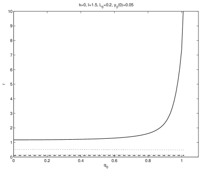
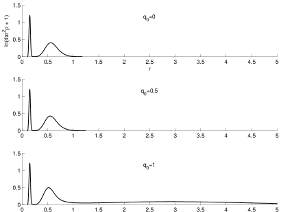
Figure 1: Shell configurations, strictly increasing $R$

4 Characterization of steady states

In this section we study the behavior of the uncharged energy density $\rho$ as a function of the area radius when the parameter for electric charge is varied. We find profiles which are multi-peaked, where the peaks are separated either by vacuum or a thin atmosphere. In this respect our results are qualitatively similar to the chargeless case, but the value of the charge parameter $q_{0}$ does affect the number of peaks in some cases. On the other hand, we find that for a sufficiently large value of the charge parameter there are no physically meaningful solutions. This is intuitively clear in view of the Newtonian case where no steady states of finite mass exist when the effective force is repulsive.

The steady states for charged matter largely follow the same basic structures as noted in [5] for the non-charged case, i.e., we get steady states with support for $\rho$ in $[R_{0},R]$, $R_{0}>0$, called shell configurations, and states where $R_{0}=0$, called ball configurations.

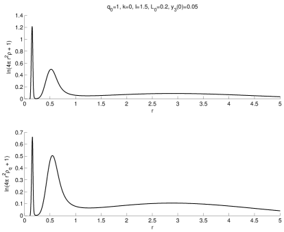
Figure 2: $\ln{(4\pi r^{2}\rho+1)}$ and $\ln{(4\pi r^{2}\rho_{q}+1)}$ for a shell configuration

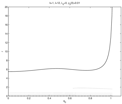
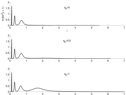
Figure 3: Ball configurations, decreasing $R$

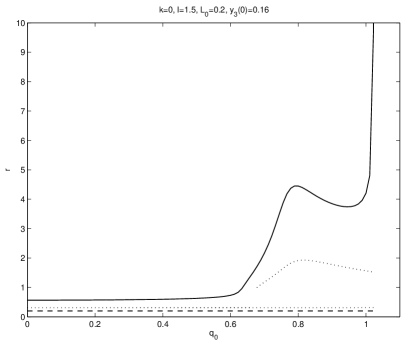
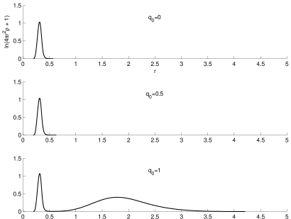
Figure 4: Shell configurations, decreasing $R$

To visualize the steady states, for each quadruple $(k,l,L_{0},y_{3}(0))$ a figure containing two subfigures is presented. Subfigure (a) shows starting points, stopping points, i.e., the inner and outer boundaries of the matter shells, as well as maxima of $\rho$ for $q_{0}\in[0,q_{0,c}[$, while subfigure (b) shows individual solutions for three values of $q_{0}$, namely $q_{0}=0,0.5,1.0$. The starting points in subfigure (a) are shown as dashed lines, the stopping points as solid lines and peaks are represented by dotted lines. The plots complement each other, the plot for the starting and stopping points contains little information on the shape of the steady states, while vacuum regions can be difficult to notice in the plots for individual solutions. To remedy the fact that peaks for $\rho$ closer to $r=0$ are in general much larger in magnitude than peaks farther out, $\ln(4\pi r^{2}\rho+1)$ rather than $\rho$ has been plotted against $r$ for the individual solutions. It should be borne in mind that this has the effect that the positions of (and in one case also number of) maxima in subfigures (a) and (b) differ.

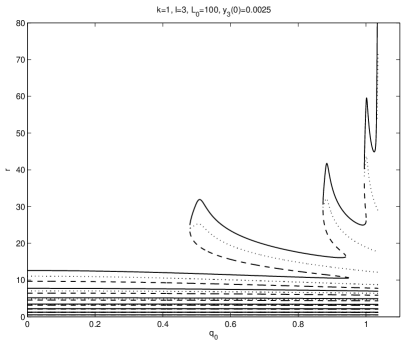
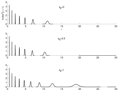
Figure 5: Multi-shell configurations, extra shells appears

The most noticeable effect of changing the particle charge $q_{0}$ is that as $q_{0}$ approaches a critical value $q_{0,c}$, the outer radius $R$ of the support for $\rho$ increases dramatically, as can be seen in Figures 1 and 3–5. Intuitively, this is expected, since for some value of $q_{0}$, the repulsive forces between individual particles from electric charge balances the attractive forces of gravity. For values of $q_{0}$ larger than $q_{0,c}$, the numerical solution breaks down since at some point $y_{2}(r)$ approaches infinity. Thus we cannot have arbitrarily large particle charge and still obtain a solution. In Figure 2 the behaviour of $\ln{(4\pi r^{2}\rho+1)}$ and $\ln{(4\pi r^{2}\rho_{q}+1)}$ is displayed. Recall here the definition of $\rho_{q}$ in (2.18). As can be seen the profiles of these quantities are similar. This observation applies to other cases in this paper as well which is the reason why we only focus on $\ln{(4\pi r^{2}\rho+1)}.$

The value of $q_{0,c}$ for fixed values of $k,l$ and $L_{0}$ varies with $y_{3}(0)$ as can be seen in Figure 6.

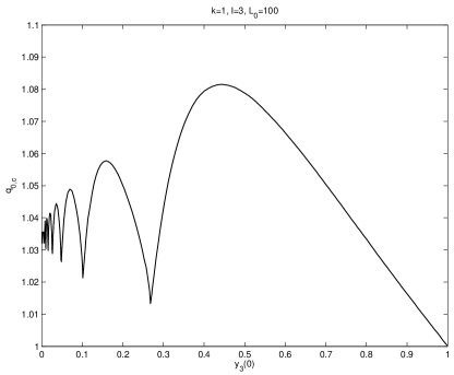
Figure 6: $q_{0,c}$ as a function of $y_{3}(0)$

We see that $q_{0,c}(y_{3}(0))$ has an undulating quality with increasing amplitude and decreasing frequency of oscillation for larger $y_{3}(0)$. As $y_{3}(0)\to 1$, we do always have that $q_{0,c}\to 1$. This is easily understood, since in the Newtonian case the critical particle charge is exactly $1$, and in the limit $y_{3}(0)\to 1$ the solutions become essentially Newtonian; notice that $1/y_{3}(0)-1$ is the central redshift factor [5, Eqn. (2.20)] which is a measure for how relativistic the system is. At any point where $\rho$ equals zero, a Reissner-Nordström solution with appropriate initial values can be joined to form a steady state with finite support. The above limit for $q_{0}$ thus only applies to situations where the distribution function is given by a single expression on the entire domain interval $r\in[0,\infty[$.

Figure 1 shows a double-peaked, single-shelled shell configuration ($k=0,l=1.5,L_{0}=0.2,y_{3}(0)=0.05$). The positions and magnitudes of peaks are virtually unaffected by the value of $q_{0}$ and the only effect that can be seen is that the tail grows in length and magnitude. The outer radius $R$ increases strictly monotonically. In Figure 3 a double-peaked ball configuration with parameters ($y_{3}(0)=0.01,k=1,l=12,L_{0}=0$) is displayed. Here we see that as $q_{0}$ increases, an extra maximum of $\rho$ appears. In this case $R$ does not increase strictly monotonically, as a decrease can be seen before the outer radius finally blows up as $q_{0}$ approaches $q_{0,c}$. Solutions in which a new shell appears and with strictly increasing $R$ can however be constructed. Although barely noticable in Figure 3, the radial position of the new maximum that appears for larger $q_{0}$ will increase at first and then decrease. This effect is more pronounced in Figure 4, however. The aforemensioned case is displaying the same behavior as in Figure 3, this time for a single-peaked shell configuration ($y_{3}(0)=0.16,k=0,l=1.5,L_{0}=0.2$). For higher values of $L_{0}$ multi-shelled configurations (i.e., configurations with multiple peaks, separated by vacuum regions), can be obtained. The effect on these is that as $q_{0}$ increases, one or more additional shells appear as can be seen in Figure 5 ($y_{3}(0)=0.0025,k=1,l=3,L_{0}=100$). These newly appearing shells mimic the behavior of the newly appearing peak in Figure 4. In Figure 5 it can be seen clearly that all peaks, except the innermost one, that are present at $q_{0}=0$ are showing an inclination to move towards $r=0$. This behavior is also present in all cases with more than one peak, although not noticable in the plots. The innermost peak, on the other hand, has a contrary tendency to move outwards.

5 Sharpness issues of the main inequality

The purpose of this section is to investigate aspects concerning sharpness of the inequality

$$\sqrt{m_{g}(r)}\leq\dfrac{\sqrt{r}}{3}+\sqrt{\dfrac{r}{9}+\dfrac{q^{2}(r)}{3r}}$$ (5.1)

where $m_{g}$ is the total gravitational mass given by

$$m_{g}(r)=4\pi\int_{0}^{r}\eta^{2}\rho(\eta)d\eta+\left(\int_{0}^{r}\dfrac{q^{2}(\eta)}{2\eta^{2}}d\eta+\dfrac{q^{2}(r)}{2r}\right)=:m_{i}+m_{q}.$$ (5.2)

This inequality was derived in [2] and it was shown to hold for any static solution of the Einstein-Maxwell-matter system which satisfies (1.2). In addition it was assumed that the solutions satisfy

$$q\leq m_{g},\;m_{g}+\sqrt{m_{g}^{2}-q^{2}}<r.$$ (5.3)

The latter conditions are imposed to ensure that the solutions are physically meaningful, cf. [10]. To better understand the motivation for our study we recall the results in the uncharged case.

If $Q=0$ the inequality (5.1) reduces to the Buchdahl inequality

$$\frac{m(r)}{r}\leq\frac{4}{9},$$ (5.4)

which was first proved in [7] under the Buchdahl assumptions that the pressure is isotropic and the energy density is non-increasing outwards. The inequality was then shown to hold independently of the Buchdahl assumptions [3] for solutions which satisfy the energy condition $p+2p_{T}\leq\rho.$ A different proof was later given in [12]. The advantage of the latter method is that the proof is shorter and more flexible since it allows for other energy conditions than (1.2). The disadvantage lies in the issues of sharpness and construction of the saturating solution. Firstly, the method does not imply that the class of saturating solutions is unique, and secondly, it is not clear that a solution to a coupled Einstein-matter system can have the properties of the saturating solution constructed in [12]. In particular solutions to the Einstein-Vlasov system are ruled out. These issues have however affirmative answers. Uniqueness is obtained in [3] where it is proved that a saturating solution must be an infinitely thin shell solution. In [4] it is shown that regular, arbitrarily thin shell solutions of the Einstein-Vlasov system exist, which implies that there are steady states to this system with $M/R$ arbitrarily close to $4/9.$

Let us now return to the charged case and discuss the latter two issues. The proof of (5.1) in [2] is based on the method in [12] and the method in [3] does not apply. A proof based on the latter method would imply uniqueness of the saturating solution, and it is thus natural to ask if there is another class than infinitely thin shell solutions with this property. Also, although the result in [2] shows that infinitely thin shell solutions saturate the inequality there is no analogous result to [4] in the charged case, i.e., the question whether or not the Einstein-Vlasov-Maxwell system admits arbitrarily thin shell solutions is open. Below we will present numerical evidence that the system does admit arbitrary thin shell solutions and in addition that another class of saturating solutions does exist.

We introduce the quantity

$$\Gamma:=\sup_{r\geq 0}\dfrac{\sqrt{m_{g}(r)}}{\dfrac{\sqrt{r}}{3}+\sqrt{\dfrac{r}{9}+\dfrac{q^{2}(r)}{3r}}},$$

which in terms of the functions introduced in (3.7) reads

$$\Gamma=\sup_{r\geq 0}\dfrac{3\sqrt{2}}{2}\dfrac{\sqrt{1-y_{2}^{-1}(r)+4\pi r^{2}y_{1}^{2}(r)}}{1+\sqrt{1+12\pi r^{2}y_{1}^{2}(r)}}.$$

By (5.1), $\Gamma$ is subject to the inequality

$$\Gamma\leq 1.$$ (5.5)

In Figure 7 the numerical results for a shell configuration with $(k=1,l=1,L_{0}=10)$ are displayed as follows. $\Gamma$ as a function of $y_{3}(0)$ is displayed in ascending order for

$$q_{0}\in\{0,0.25,0.5,0.75,0.999,1.001,1.25,1.5\},$$

the bottom-most curve being that for $q_{0}=0$, the next to bottom-most being that for $q_{0}=0.25$ and so on. In all cases tested for other parameter values, $\Gamma(y_{3}(0))$ falls within the first shell of the solution.

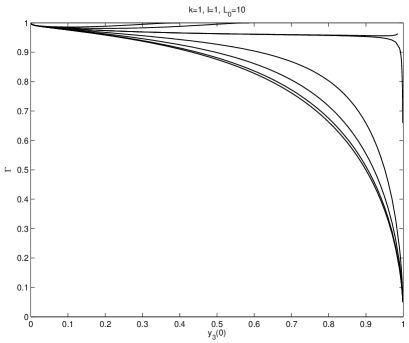
Figure 7: $\Gamma$ as a function of $y_{3}(0)$ for a shell configuration

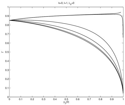
Figure 8: $\Gamma$ as a function of $y_{3}(0)$ for a ball configuration

We see that as $y_{3}(0)$ approaches zero (5.5) approaches equality for all values of $q_{0}$. By letting $R_{11}$ be the outer radius of the first shell and plotting the ratio $R_{11}/R_{0}$ in Figure 9,

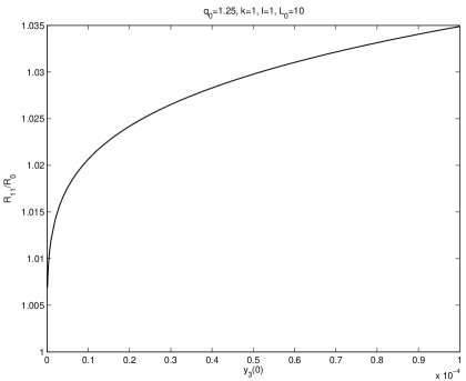
Figure 9: $R_{11}/R_{0}$ as a function of $y_{3}(0)$

we see that in the limit $y_{3}(0)\to 0$, $R_{11}/R_{0}\to 1$, i.e., we find numerical support that the Einstein-Vlasov-Maxwell system admits arbitrarily thin shell solutions. For values of $q_{0}\leq 1$, we see that $\Gamma(y_{3}(0))$ is monotonically decreasing, and as $y_{3}(0)$ approaches unity, $\Gamma$ approaches zero. This, however, is not the case for $q_{0}>1$ where $\Gamma(y_{3}(0))$ will at some point start increasing. For values of $q_{0}$ slightly larger than $1,$ $\Gamma$ will not increase rapidly enough for (5.5) to once again be saturated. For larger values of $q_{0}$, (5.5) will however be saturated a second time, cf. Figure 10 where the graph for the case with $q_{0}=1.25$ is depicted using a different scale on the $\Gamma-$axis. From Figure 11 it is clear that this occurs when $Q=M=R$. Hence, in the charged case the class of saturating solutions is not unique. Figure 12 displays the graph of $\rho$ for a solution which nearly saturates the inequality and such that $M,Q$ and $R$ are almost equal, and we see that it is indeed not a thin shell solution. In equation (5.2) the quantities $m_{i}$ and $m_{q}$ were defined, and roughly they represent the parts of the gravitational mass induced by $\rho$ and $q$ respectively. However, it should be noted that the nonlinearity of the equations make it impossible to completely separate the influences of these quantities. In figure 13 these quantities are plotted in three different cases. Note in particular that in the third case, which corresponds to the saturating solution for which $M=Q=R,$ $m_{i}$ and $m_{q}$ are almost equal at the outer boundary of the solution.

Figure 8 shows $\Gamma(y_{3}(0))$ for the family of ball configurations with $(k=0,l=1,L_{0}=0)$, for $q_{0}=\{0,0.25,0.50,0.75,0.999,1.001\}$.

Although no longer monotonically decreasing, $\Gamma(y_{3}(0))$ approaches zero as $y_{3}(0)$ approaches unity for $q_{0}<1$, as in the case for the above shell configurations.

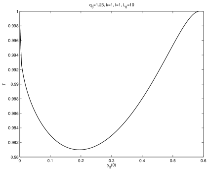
Figure 10: $\Gamma$

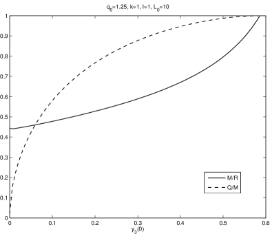
Figure 11: $Q/M$ and $M/R$ as functions of $y_{3}(0)$

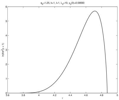
Figure 12: The profile of a saturating solution which is not a thin shell

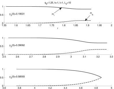
Figure 13: The relation between $m_{i}$ and $m_{q}$

6 Spirals in the mass radius diagram

In this section we study the behavior of the total gravitational mass $M$ and outer radius of the support $R$ for one parameter families of steady states. The parameter is $y_{3}(0)$ while $k,l,L_{0}$ and $q_{0}$ are kept constant. In [5] it has been shown that in the isotropic (i.e., $l=L_{0}=0$) and chargeless case, $(R,M)$ forms a spiral. Furthermore, numerical evidence is given that this is also the case for non-isotropic solutions. Charged matter, as studied in this paper, displays the same behavior and changing $q_{0}$ merely deforms the spirals. This can be seen in Figures 14 and 15 showing the $(R,M)$-spirals for $q_{0}=0$ and $q_{0}=0.5$ with ($k=1,l=5,L_{0}=2$).

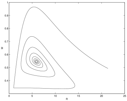
Figure 14: $(R,M)$-spiral, $q_{0}=0$

We see that increasing $q_{0}$ from $0$ to $0.5$ does not change the shape significantly. These characteristics are displayed for all combinations of $k,l$ and $L_{0}$.

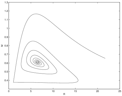
Figure 15: $(R,M)$-spiral, $q_{0}=0.5$

The sharp corner in these mass-radius spirals is a genuine feature, since for $L_{0}>0$ the radius of the support as $y_{3}(0)$ varies can change discontinuosly due to new shells which appear, cf. [5, p. 1829].

So far in this paper we have only used the ansatz (3.14)for the distribution function. Only the analogous ansatz is used in [5], so it might be interesting to see if the $(R,M)$-spirals are also a feature of other ansatz functions of the form $f(r,w,L)=\phi(E/E_{0},L)$. For instance, with $\phi(E/E_{0},L)=\sin^{2}\left(k(1-E/E_{0})_{+}\right)\sin^{2}\left(l(L-L_{0})_{+}\right)$, and ($k=2,l=3,L_{0}=1$, $q_{0}=0.5$), we get the spiral in Figure 16. For all cases tested, we do in fact get $(R,M)$-spirals. We conclude that $(R,M)$-spirals are a general feature of the Einstein-Vlasov-Maxwell system with the ansatz $f(r,w,L)=\phi(E/E_{0},L)$.

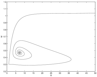
Figure 16: ($R,M)$-spiral, $q_{0}=0.5$, alternative ansatz

References

- [1] H. Andréasson, The Einstein-Vlasov system/Kinetic theory, Liv. Rev. Relativity 8 (2005).
- [2] H. Andréasson, Sharp bounds on the critical stability radius for relativistic charged spheres. To appear in Commun. Math. Phys. arXiv:0804.1882.
- [3] H. Andréasson, Sharp bounds on of general spherically symmetric static objects. J. Diff. Equations 245, 2243-2266 (2008).
- [4] H. Andréasson, On static shells and the Buchdahl inequality for the spherically symmetric Einstein-Vlasov system. Commun. Math. Phys. 274, 409–425 (2007).
- [5] H. Andréasson, G. Rein, On the steady states of the spherically symmetric Einstein-Vlasov system. Class. Quantum Grav. 24, 1809-1832 (2007).
- [6] P. Anninos, T. Rothman, Instability of extremal relativistic charged spheres. Phys. Rev. D, 62 024003 (2001).
- [7] H. A. Buchdahl, General relativistic fluid spheres. Phys. Rev. 116, 1027–1034 (1959).
- [8] F. de Felice, L. Siming, and Y. Yunqiang, Relativistic charged spheres: II. Regularity and stability. Class. Quantum Grav. 16, 2669-2680 (1999).
- [9] C. J. Farrugia, P. Hajicek, The third law of black hole mechanics: A counterexample. Commun. Math. Phys. 68, 291-299 (1979).
- [10] A. Giuliani, T. Rothman, Absolute stability limit for relativistic charged spheres, Gen. Rel. Gravitation DOI 10.1007/s10714-007-0539-7 (2007).
- [11] M. Heinzle, N. Röhr and C. Uggla, Dynamical systems approach to relativistic spherically symmetric static perfect fluid models. Class. Quantum Grav. 20, 4567-4586 (2003).
- [12] P. Karageorgis, J. Stalker, Sharp bounds on for static spherical objects. Class. Quantum Grav. 25, 195021 (2008).
- [13] T. Makino, On the spiral structure of the -diagram for a stellar model of the Tolman-Oppenheimer-Volkoff equation. Kunkcialaj Ekvacioj 43, 471–489 (2000)
- [14] G. Rein, A. D. Rendall, Compact support of spherically symmetric equilibria in non-relativistic and relativistic galactic dynamics. Math. Proc. Camb. Phil. Soc. 128, 363–380 (2000).