Collision statistics in sheared inelastic hard spheres

Abstract

The dynamics of sheared inelastic-hard-sphere systems are studied using non-equilibrium molecular dynamics simulations and direct simulation Monte Carlo. In the molecular dynamics simulations Lees-Edwards boundary conditions are used to impose the shear. The dimensions of the simulation box are chosen to ensure that the systems are homogeneous and that the shear is applied uniformly. Various system properties are monitored, including the one-particle velocity distribution, granular temperature, stress tensor, collision rates, and time between collisions. The one-particle velocity distribution is found to agree reasonably well with an anisotropic Gaussian distribution, with only a slight overpopulation of the high velocity tails. The velocity distribution is strongly anisotropic, especially at lower densities and lower values of the coefficient of restitution, with the largest variance in the direction of shear. The density dependence of the compressibility factor of the sheared inelastic hard sphere system is quite similar to that of elastic hard sphere fluids. As the systems become more inelastic, the glancing collisions begin to dominate more direct, head-on collisions. Examination of the distribution of the time between collisions indicates that the collisions experienced by the particles are strongly correlated in the highly inelastic systems. A comparison of the simulation data is made with DSMC simulation of the Enskog equation. Results of the kinetic model of Montanero et al. [Montanero et al., J. Fluid Mech. 389, 391 (1999)] based on the Enskog equation are also included. In general, good agreement is found for high density, weakly inelastic systems.

I Introduction

In rapid granular flows Campbell (1990); Goldhirsch (2003), the mean flight time of the particles in the granular material may be large compared to the contact time between particles. Inter-particle interactions are modelled as “collisions,” which play a key role in transferring momentum and other properties through the system. Granular materials in this flow regime can then be represented by a collection of inelastic hard spheres Campbell and Brennen (1985); Lutsko (2004a).

The simplicity of the inelastic hard sphere model lends itself well to theoretical analysis. In particular, the methods developed for the kinetic theory of equilibrium gases have been applied to rapidly sheared inelastic hard sphere systems. The seminal paper by Lun et al. Lun et al. (1984) marked the start of “complete” kinetic theories capable of predicting both the kinetic and collisional properties. The Boltzmann equation has featured predominantly in the theory of granular gases due to its simpler form (e.g., see Ref. Santos and Astillero (2005)); however, the most successful molecular kinetic theory to date is the revised Enskog theory van Beijeren and Ernst (1973), an extension to the Boltzmann equation for dense systems. Enskog theory assumes uncorrelated particle velocities and currently relies on a static structrual correlation factor from elastic fluids Carnahan and Starling (1969). Approximate theories beyond the Enskog theory, such as ring theory van Noije et al. (1998), have been developed and applied to granular systems, however, due to their complexity, their use has been limited (e.g., cooling, rare granular gases).

Common to most kinetic theory solutions is the assumption of a steady state, spatially uniform distribution function. Provided scale separation exists, as is the case for elastic fluids, fluctuations from this steady state can be accounted for using the Chapman-Enskog expansion Sela and Goldhirsch (1998). To solve the Enskog equation, approximations typically begin by taking moments of the kinetic equation with respect to the density, velocity, and products of the velocity. These moment equations are used to solve for the parameters of an expansion or model. Typically, only terms up to the granular “temperature”, or isotropic stress and rotation terms Lun (1991), are included as field variables. Anisotropic stresses can still be predicted from such a theory Goldhirsch (2008); indeed, attempts have been made to include the full second order velocity moment Jenkins and Richman (1988) as a hydrodynamic variable to improve theoretical predictions.

Grad’s method Jenkins and Richman (1985) solves Enskog theory using an expansion of the distribution function about a reference state. This has been applied to poly-disperse granular systems Lutsko (2004a) and, unlike perturbative solutions, does not require assumptions on the strength of the shear. Kinetic models are a powerful method of generating simplified kinetic equations which retain key features of the original. Montanero et al. Montanero et al. (1999) solved an improved Bhatnagar-Gross-Krook (BGK) kinetic model Santos et al. (1998); Brey et al. (1999) for inelastic systems. The improved BGK model approximates the collisional term of the kinetic equation using the first two velocity moments, which correspond to the collisional stress and energy loss, and a general relaxation term. This leads to a simplified kinetic equation. The solution in the low dissipation limit is particularly attractive, as it provides estimates for the system properties without requiring numerical solution and compares favourably to Direct Simulation Monte Carlo (DSMC) results.

DSMC Bird (1994) is a numerical simulation technique to directly solve the Boltzmann equation without requiring further approximations. This can then be used to rapidly test solutions of the kinetic equation. The method has already been extended to the Enskog equation for homogeneously sheared inelastic systems Hopkins and Shen (1992); Montanero and Santos (1997); Montanero et al. (1999).

While kinetic theories do offer insight into the behavior of granular materials, they are necessarily approximate. The Boltzmann and Enskog kinetic theories do not include velocity or dynamic structural correlations. Ring theory van Noije et al. (1998) is capable of including particle correlations; however, further approximations are required to make the resulting theory tractable. These correlations are present in moderately dense to dense systems of elastic particles, but they are enhanced by the clustering in inelastic systems Alam and Luding (2003); M. and S. (2005). The failure of Boltzmann and Enskog theories at high densities is therefore expected, even for elastic hard sphere systems. On the other hand, non-equilibrium molecular dynamics (NEMD) simulations Campbell (1989); Campbell and Brennen (1985) can, in principle, give “exact” results for driven inelastic-hard-sphere systems Herbst et al. (2004); Herrmann et al. (2001). These simulations can be used to validate kinetic theories against the underlying model. Initial studies of sheared granular systems used moving boundaries Campbell and Brennen (1985); Conway and Glasser (2004), such as rough walls, to introduce energy into the system. Due to the computational limitations, the wall separation is typically of the order of a few particle diameters, and wall effects dominate the simulation results. For large system sizes, shear instability is observed Alam et al. (2005). Consequently, the results for wall driven simulations are strongly dependent on system size.

Another manner to introduce shear in non-equilibrium molecular dynamics is the Lees-Edwards Lees and Edwards (1972) or “sliding brick” boundary conditions. Simulations of inelastic hard-sphere systems using Lees-Edwards boundary conditions Walton and Braun (1986); Campbell (1989); Hopkins and Louge (1991); Goldhirsch and Tan (1996); Tan and Goldhirsch (1997) lessen the influence of wall effects, by elimination of the surface of the system, but these simulations still introduce shear in an inhomogenous manner, which leads to clustering instabilities Lutsko (2004b) for larger systems.

While there are many interesting similarities between elastic hard-sphere fluids and driven inelastic hard-sphere systems, there are key differences. One is the tendency of inelastic hard spheres to form clusters and patterns, while elastic hard sphere fluids tend to remain isotropic. Another example is the velocity distribution. The velocity of elastic hard spheres is governed by the Maxwell distribution, which is isotropic and Gaussian. The velocity distribution of flowing inelastic hard spheres is, in general anisotropic Losert et al. (1999), and can show significant deviations from the Gaussian distribution, especially when there is clustering.

In this work, we examine the properties of sheared inelastic-hard-sphere systems using non-equilibrium event-driven molecular dynamics simulations with the SLLOD algorithm combined with Lees-Edwards boundary conditions. Part of the purpose of this work is to investigate, at a particle level, the differences between the behavior of inelastic and elastic (equilibrium) hard sphere systems. Another purpose of this work is to provide simulation data which can be used to test kinetic theory predictions for the properties of these systems. A previous study by Montanero et al. Montanero et al. (2006) has already compared 2D and 3D simulations of binary inelastic hard spheres against DSMC simulations of Enskog theory. They find good agreement over the range of mass ratio, size ratio and inelasticity studied; however, the clustering instability present in systems of large numbers of highly inelastic particles appears to limit the range of inelasticity studied. As mentioned previously, kinetic theories for sheared granular materials are typically developed for the case where the system is spatially uniform and homogeneously sheared. One of the difficulties with comparing the predictions of the kinetic theory with the simulation data for sheared granular materials is the formation of clusters, which makes comparison between the two problematic. As a consequence, care is taken in this work to ensure that the systems remain homogeneous and strongly inelastic systems can be accessed. In these simulations, we investigate the collision statistics, such as velocity distributions, collision angles, time between collisions and mean free paths, of sheared inelastic hard spheres. In addition, we examine the variation of various bulk properties of the system, such as the viscosity, mean kinetic energy, and stress, with the packing fraction and coefficient of restitution of the particles. We also investigate the correlations between the collisions, which are neglected in most kinetic theory approaches. The remainder of this paper is organized as follows. In Section II, we describe the details of the granular dynamics simulations. In Section III, we describe the details of the DSMC simulations. In Section IV, we present the results of our simulation work, including a comparison with the predictions of Enskog theory. Finally, a summary of the main findings is provided in Section V.

II Simulation details

Non-equilibrium granular dynamics simulations were performed on systems of inelastic hard spheres of diameter $\sigma$ and mass $m$. The system is sheared in the $y$-plane in the $x$-direction with a constant strain rate of $\dot{\gamma}$ using the SLLOD algorithm Evans and Morris (1990). In this method, shear is applied through the use of the Lees-Edwards sliding brick boundary conditions Lees and Edwards (1972); Evans and Morris (1990) and the velocity is transformed relative to a linear velocity profile. The equations of motion are

$$\frac{d{\bf r}_{i}}{dt}= \bar{\bf v}_{i}+y_{i}\dot{\gamma}\hat{\bf e}_{x}$$ (1)

$$\frac{d\bar{\bf v}_{i}}{dt}= \frac{{\bf F}_{i}}{m}-\bar{v}_{y,i}\dot{\gamma}\hat{\bf e}_{x}$$ (2)

where ${\bf F}_{i}$ is the force acting on particle $i$, ${\bf r}_{i}$ is the position of particle $i$, $\bar{\bf v}_{i}$ is the so called peculiar velocity of particle $i$, $y_{i}$ is the $y$-coordinate of particle $i$, $\bar{v}_{y,i}$ is the $y$-component of the peculiar velocity of particle $i$, $\hat{\bf e}_{x}$ is a unit vector pointing in the positive $x$-direction, and $\dot{\gamma}$ is the strain rate.

The peculiar velocity of a particle $i$ is defined as the difference between its lab velocity ${\bf v}_{i}$ and the local streaming velocity (the velocity of the local streamline). For simple shear, it is given by the linear transformation

$$\bar{\bf v}_{i}={\bf v}_{i}-y_{i}\dot{\gamma}_{i}\hat{\bf e}_{x}$$

The peculiar velocity is related to the dispersion of the particles from the average streamlines of the flow. The SLLOD equations of motion are particularly convenient as the peculiar velocity is naturally recovered without the need for a separate co-ordinate transformation. They allow the possibility of thermostatting the system Petravic and Jepps (2003) and the study of time dependent shear flows.

In a hard-sphere system, the spheres do not experience any force between collisions. The equations of motion can then be solved analytically for the trajectories of the spheres between collisions. The evolution of the position and peculiar velocity of particle $i$ in the system between collisions is

$${\bf r}_{i}(t)= {\bf r}_{i}(t_{0})+[\bar{\bf v}_{i}(t_{0})+y_{i}(t_{0})\dot{\gamma}\hat{\bf e}_{x}](t-t_{0})$$

$$= {\bf r}_{i}(t_{0})+{\bf v}_{i}(t_{0})(t-t_{0})$$

$$\bar{\bf v}_{i}(t)= \bar{\bf v}_{i}(t_{0})-\bar{v}_{y,i}(t_{0})\dot{\gamma}(t-t_{0})\hat{\bf e}_{x}$$ (3)

When a particle undergoes a collision, it experiences an impulse which alters its velocity. These collisions are instantaneous and only occur between pairs of spheres (i.e., there are no three or higher body collisions). The inelasticity of the hard spheres is characterized by the coefficient of restitution $\alpha$. This is defined through the amount of kinetic energy $\Delta{E}$ lost on collision

$$\Delta{E}=\frac{m}{4}(1-\alpha^{2})\left(\hat{\bf r}_{ij}\cdot{\bf v}_{ij}\right)^{2}$$ (4)

where ${\bf v}_{i}$ is the velocity of particle $i$ immediately before collision, ${\bf v}_{ij}={\bf v}_{i}-{\bf v}_{j}$, and $\hat{\bf r}_{ij}={\bf r}_{ij}/|{\bf r}_{ij}|$ is the unit vector pointing from the center of particle $j$ to the center of particle $i$.

Each collision preserves the total momentum of the particles involved; therefore, the change of velocities for a colliding pair of spheres $i$ and $j$ is given by

$${\bf v}_{i}^{\prime}= {\bf v}_{i}-\frac{1}{2}(1+\alpha)\left(\hat{\bf r}_{ij}\cdot{\bf v}_{ij}\right)\hat{\bf r}_{ij}$$

$${\bf v}_{j}^{\prime}= {\bf v}_{j}+\frac{1}{2}(1+\alpha)\left(\hat{\bf r}_{ij}\cdot{\bf v}_{ij}\right)\hat{\bf r}_{ij}$$ (5)

where the primes denote post collision values of the particle velocities.

The coefficient of restitution $\alpha$ is, in general, a function of the relative velocity on collision. Viscoelastic models that incorporate this have been very successful in describing real systems such as steel spheres McNamara and Falcon (2003). A common approximation in kinetic theory is to assume a constant coefficient of inelasticity, as this greatly simplifies the collision integrals while the basic physics is not significantly altered. A constant coefficient of restitution is used in this work to facilitate comparison against kinetic theory results.

One concern for a system with a constant coefficient of restitution is the phenomenon of inelastic collapse, where an infinite number of collisions occur between several spheres in a finite interval of time. Event-driven simulations will fail in the event of a single collapse event. In two dimensional, freely cooling, inelastic hard sphere systems undergo McNamara and Young (1996) inelastic collapse with coefficient of restitution as high as 0.59.

Inelastic collapse is rare in sheared systems Alam and Hrenya (2001) and is increasingly rare in higher dimensions; however, a near collapse situation can still cause a simulation to break down if the machine precision is not sufficiently high to resolve a rapid series of successive collisions. In the simulations performed in this work, no partial or full collapse events were found, even for dense and highly inelastic systems.

The simulation algorithm that we employ is a generalization of the standard event-driven molecular dynamics algorithm for hard spheres Alder and Wainwright (1959) (see Ref. Bannerman and Lue (2008)). The main modifications are the use of the sliding brick boundary conditions Lees and Edwards (1972) and the SLLOD equations of motion.

Unlike the elastic hard sphere system, the inelastic hard-sphere system has no intrinsic time scale. The applied strain rate $\dot{\gamma}$ sets the time scale of the system. Therefore, there are only two relevant dimensionless parameters: the density $\rho\sigma^{3}$ and the coefficient of restitution $\alpha$. In this work, the density is varied from $\rho\sigma^{3}=0.4$ to $0.9$, and the coefficient of restitution is varied from $\alpha=0.4$ to $0.9$.

Because the shear is imposed through the boundary conditions, the strain rate is only fixed at two points, separated by the entire height of the simulation box. In low density systems with large numbers of particles, clustering occurs Alam et al. (2005). This leads to a local variation of the strain rate in the system, and, consequently, the system will not be homogeneously sheared. At the onset of clustering, the size dependence of the system properties changes from the typical $N^{-1}$ scaling to a different behavior. To illustrate this, the mean free time of sheared inelastic-hard-spheres with $\alpha=0.4$ is shown in Fig. 1. These simulations were performed in a cubic simulation box where the system size was varied while holding the density constant. The “break” in the curves for the lower densities indicates the presence of cluster formation in the larger systems. The same general behavior manifests in all system properties and is relatively easy to detect.

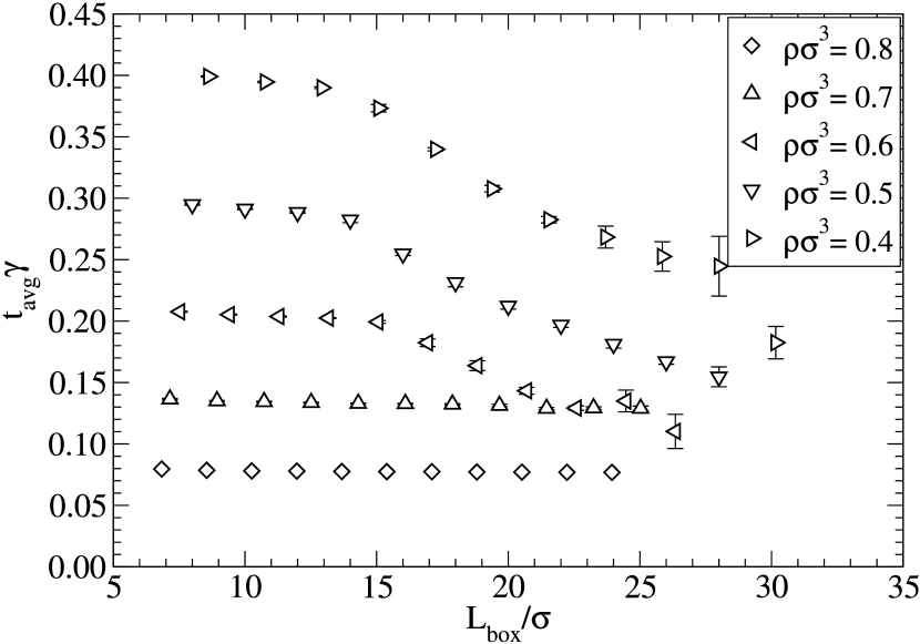
Figure 1: The system size dependence of the mean free time between collisions ${\rm t}_{\rm avg}$ for simulations of a sheared, inelastic hard sphere system with $\alpha=0.4$ in a cubic box with sides of length $L_{\rm box}$. The number of particles is $N=256$ in the smallest system and $N=10,976$ in the largest.

Kinetic theory studies of sheared inelastic systems typically assume that the system is homogeneous and uniformly sheared, with a linear velocity profile. This makes the comparison between granular dynamics simulations and the kinetic theory problematic. To allow comparison with these theories, we ensure that the systems remain homogeneous during the course of the simulations. In order to avoid the clustering regime while still maintaining a large system size to provide proper statistics, the $x$-, $y$-, and $z$-dimensions of the simulation box are set to the ratio $14.4:1:1$ and there are a total $N=7200$ spheres. This ensured that the systems remained homogeneous for all conditions (i.e. number of particles, coefficient of restitution, and density) that were examined in this work.

At the beginning of the simulations for each set of conditions, the spheres are arranged in a face centered cubic lattice at the appropriate density. The velocities of the spheres are initially assigned from a Maxwell-Boltzmann distribution. The simulations are then run for an “equilibration” period of $10^{7}$ collisions. Afterwards, system property data are collected over at least $10$ production runs, each lasting $10^{7}$ collisions. The uncertainties of the data are estimated from the standard deviations of the results from these separate runs. In the next section, we describe the DSMC simulations performed.

III DSMC Simulations

The DSMC method was used to numerically solve the Enskog equation. This technique has been described in detail previously Hopkins and Shen (1992); Montanero et al. (1999) and is only covered briefly here. The peculiar velocity distribution function $f$ is represented by using a collection of $N$ sample velocities or “simulated” particles:

$$f(\bar{\bf v},t)={N}^{-1}\sum_{i=1}^{{N}}\delta^{3}\left(\bar{\bf v}-\bar{\bf v}_{i}(t)\right),$$ (6)

where $\bar{\bf v}_{i}(t)$ is the peculiar velocity of sample $i$ at time $t$. At each time step $\Delta t$, the samples are evolved according to the SLLOD dynamics (see Eq. (2)). The samples are then tested for collisional updates. At each time step, $\frac{1}{2}{N}P_{\rm max}^{(c)}$ pairs of samples in the collection are selected, where $P_{\rm max}^{(c)}$ is a parameter of the DSMC simulation. The probability that a collision between a pair of samples $i$ and $j$ will be executed is proportional to

$$P_{ij}^{(c)}=4\pi\sigma^{2}\chi\rho\left(\hat{\bf k}\cdot{\bf v}_{ij}\right)\Theta\left(\hat{\bf k}\cdot{\bf v}_{ij}\right)\Delta t$$ (7)

where $\hat{\bf k}$ is a randomly generated unit vector, ${\bf{}v}_{ij}=\bar{\bf{}v}_{i}-\bar{\bf{}v}_{i}-\sigma\dot{\gamma}\hat{k}_{y}\hat{\bf{}e}_{x}$ is the relative lab velocity, $\Theta$ is the Heaviside step function, and $\chi$ is the radial distribution function at contact. In this work, the value of $\chi$ is taken from the Carnahan-Starling Carnahan and Starling (1969) equation of state for elastic hard spheres, which is given by

$$\chi=\frac{1-\nu/2}{\left(1-\nu\right)^{3}}$$ (8)

where $\nu=\rho\pi\sigma^{3}/6$ is the solid fraction.

To optimize the simulation, the quantity $P_{\rm max}^{(c)}$ is chosen to be the maximum observed value of $P_{ij}^{(c)}$. This is estimated and updated during a simulation if $P_{ij}^{(c)}$ exceeds $P_{max}^{(c)}$. The probability that a collision between samples $i$ and $j$ is executed is $P_{ij}^{(c)}/P_{\rm max}^{(c)}$, and, if the collision is accepted, the velocities are updated using Eq. (5) with ${\bf r}_{ij}=-\sigma\hat{\bf k}$.

For the results presented here, ${N}=1372$ and $\Delta t$ is selected such that $\frac{1}{2}{N}P_{\rm max}^{(c)}<5$. The distribution functions are equilibrated for $10^{6}$ collisions, and then results are collected and averaged over $10$ runs of $10^{7}$ collisions.

IV Results and discussion

In this section, we present our simulation results for the properties of homogeneously sheared inelastic hard sphere systems. These results are compared against DSMC simulation of the Enskog equation to test the Enskog approximation. We also include the results from the kinetic model solved by Montanero et al. Dufty et al. (1997); Montanero et al. (1999). This theory is particularly interesting as it provides analytical results in the limit of small strain rates, along with simple expressions that approximate DSMC results. Without the small strain rate approximation, a more accurate numerical solution of the model is available Montanero et al. (1999); however, the DSMC simulations already provide accurate Enskog theory results without further approximation.

IV.1 Velocity distribution

The kinetic energy of the system is defined through the fluctuations of the velocity of the particles from their respective local streaming velocity

$${E}=\frac{1}{2}\sum_{k=1}^{N}m\bar{v}_{k}^{2}.$$ (9)

The mean kinetic energy is therefore a measure of the velocity dispersion present in the system. In analogy with elastic (equilibrium) hard sphere fluids, a kinetic (or “granular”) temperature $T$ is typically introduced through the relation

$$\frac{3}{2}Nk_{B}T\equiv\langle{E}\rangle,$$ (10)

where $N$ is the number of particles in the system, and $k_{B}$ is the Boltzmann constant. Although the physical significance of the “granular temperature” has been a subject of some controversy Goldhirsch (2008), the concept has proved effective in the theoretical modelling of the properties of granular materials.

The granular temperature of the sheared inelastic hard sphere system at steady state is plotted in Fig. 2. The symbols are the results of our molecular dynamics simulations, the dotted lines are the suggested expressions of Montanero et al. Montanero et al. (1999), and the solid lines are the DSMC simulation results. From the figure, it can be seen that the granular temperature of the system decreases with decreasing values of the coefficient of restitution. The particles in a strongly inelastic system rebound less from collisions; therefore, collisions in the direction of shear can quickly settle a particle to the velocity of the streamline. In addition, the motion of the particles off the streamline (in the $y$- and $z$-directions) are more quickly dissipated by collisions with particles on neighboring streamlines. Consequently, strongly inelastic systems have a greater tendency to follow the streamlines of a flow.

At low densities, the granular temperature increases with decreasing particle densities. The collisions between particles transmit information regarding the mean velocity of the flow. For very low density systems, the collisions are relatively rare events, and between collisions a particle will generally travel on trajectories that deviate from the streamlines, thus contributing to the granular temperature. With increasing density, a particle will become increasingly “caged” by surrounding particles, experiencing more collisions that will keep it on a particular streamline. Therefore, one expects that the temperature should generally decrease with increasing particle density. However, the simulation data indicate that the temperature of the system does not depend monotonically with the density, and a minimum is observed at a relatively high density for all the systems considered. The minimum becomes more pronounced as the coefficient of restitution decreases.

We note that in dense experimental granular systems, particles mainly remain in contact with each other and interact by rolling or sliding past one another, rather than through collisions. In this regime, soft sphere models Campbell (2002), as opposed to hard sphere models, are more representative. Consequently, the applicability of the simulation results for the inelastic hard sphere system at high densities to experimental granular systems should be considered with care.

In general, Enskog theory and the solution of Montanero et al. provides a fairly accurate description of the simulation results; however, there is a large discrepancy for high values of the inelasticity and density. In addition, Enskog theory does not capture the presence of the minimum in the temperature with respect to the density.

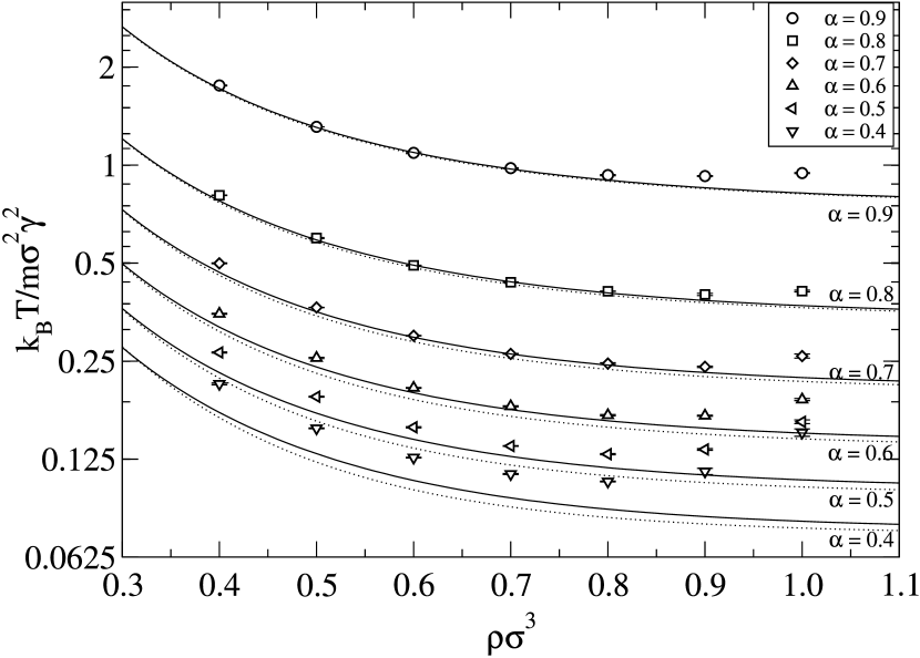
Figure 2: Variation of the mean kinetic energy per particle with density for (i) $\alpha=0.4$ (circles), (ii) $\alpha=0.5$ (squares), (iii) $\alpha=0.6$ (diamonds), (iv) $\alpha=0.7$ (triangles-up), (v) $\alpha=0.8$ (triangles-left), and (vi) $\alpha=0.9$ (triangles-down). The dotted lines are the suggested expressions of Ref. Montanero et al. (1999) and the solid lines are DSMC results.

Equilibrium fluids obey the equipartition theorem: energy is, on average, distributed evenly between all degrees of freedom. In driven granular systems, however, this has been shown to not be the case Knight and Woodcock (1996). Figure 3a shows the variation of $\langle\bar{v}_{y}^{2}\rangle/\langle\bar{v}_{x}^{2}\rangle$ with density, and Fig. 3b shows the variation of $\langle{\bar{v}_{z}^{2}\rangle/\langle\bar{v}_{y}^{2}}\rangle$. The symbols are the results of our molecular dynamics simulations, the dotted lines are the predictions of the theory of Montanero et al. Montanero et al. (1999), and the solid lines are the DSMC simulation results. If the system obeyed the equipartition function, then both these ratios would be equal to one. The dispersion of the velocity parallel to the direction of shear (i.e. the $x$-direction) is consistently larger than that perpendicular to the shear, which is unsurprising as this is the direction in which energy is inputted to the system. The asymmetry increases with decreasing density and with decreasing values of the coefficient of restitution. It is interesting to note, however, that the fluctuations in the velocity in the $y$- and $z$-directions are nearly equal.

The low dissipation theory of Montanero et al. strongly under predicts the anisotropy in the velocity dispersion. DSMC results provide a better description but still deviate significantly from the simulation results at low values of the elasticity.

Montanero et al.’s theory truncates terms within the second velocity moment of the collision integral and all higher terms. The full second moment could be included to improve predictions; however, as this is primarily a collision term it is unlikely to improve the predictions of the velocity anisotropy.

The kinetic model could be expanded by relaxing to a generalized Gaussian distribution, as in the ellipsoidal statistical model. The extra degrees of freedom in the model would then be solved for by the inclusion of a full second velocity moment balance. This might still prove tractable and improve the predictions for the velocity dispersion anisotropy.

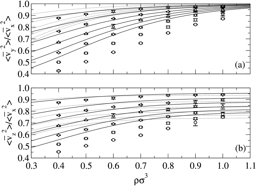
Figure 3: The ratio of the mean-squared-velocity (a) in the $y$- and $x$-directions and (b) in the $z$- and $x$-directions for sheared inelastic hard sphere sytems with (i) $\alpha=0.4$ (circles), (ii) $\alpha=0.5$ (squares), (iii) $\alpha=0.6$ (diamonds), (iv) $\alpha=0.7$ (triangles-up), (v) $\alpha=0.8$ (triangles-left), and (vi) $\alpha=0.9$ (triangles-down). The dotted lines are the suggested expressions of Ref. Montanero et al. (1999), and the solid lines are the DSMC results.

For equilibrium systems, such as elastic-hard-sphere fluids, the velocity distribution is exactly given by the Maxwell-Boltzmann distribution; however, granular materials have been shown to deviate from this distribution Olafsen and Urbach (1999); Losert et al. (1999); Rouyer and Menon (2000). The simulation data for the distributions of the single particle $x$-, $y$-, and $z$-component of the peculiar velocity are shown in Fig. 4. The peculiar velocities are reduced by their mean squared values ($v_{i}^{*}=\bar{v}_{i}/\left\langle\bar{v}_{i}^{2}\right\rangle^{1/2}$, for $i=x$, $y$, and $z$). The distributions are, in general, well described by an anisotropic Gaussian distribution. For the highly inelastic systems, the distributions display a slightly enhanced high velocity tail. This is most evident in the direction of shear (i.e. the $x$-direction).

For simulations in a cubic box at the onset of clustering in the system, the peculiar velocity distributions in the $y$- and $z$-directions can be shown to develop strong high velocity tails. In this case, the bulk of the particles are within a dense low strain rate zone, while the remainder reside in a rare, high strain rate and granular temperature region. The particles in the high strain rate region lead to a high velocity tail. Further studies on clustering effects are currently underway.

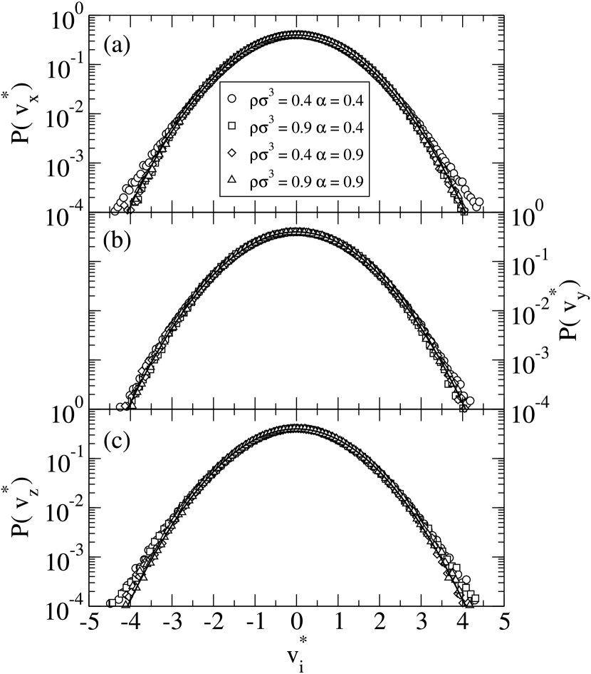
Figure 4: The peculiar velocity distribution in the (a) $x$-direction, (b) $y$-direction, and (c) $z$-direction in sheared inelastic hard sphere systems with (i) $\rho\sigma^{3}=0.4$ and $\alpha=0.4$ (circles), (ii) $\rho\sigma^{3}=0.9$ and $\alpha=0.4$ (squares), (iii) $\rho\sigma^{3}=0.4$ and $\alpha=0.9$ (diamonds), and (iv) $\rho\sigma^{3}=0.9$ and $\alpha=0.9$ (triangles). The solid line is a Gaussian distribution.

IV.2 Stress tensor

In this section, we examine the stress tensor. The time averaged value of the stress tensor $\langle{\bf P}\rangle$ for a hard-sphere system is given by Alder et al. (1970)

$$\langle{\bf P}\rangle=\frac{1}{V\tau}\sum_{{\rm collisions}}^{\tau}\left[\Delta t_{c}\sum_{k=1}^{N}m\bar{\bf v}_{k}\bar{\bf v}_{k}+\sigma\hat{\bf r}_{ij}m\Delta{\bf v}_{i}\right]$$ (11)

where $\Delta t_{c}$ is the time interval between two consecutive collisions, $\Delta{\bf v}_{i}$ is the change of velocity of sphere $i$ on collision, $\tau$ is the time over which the stress tensor is averaged, and $V$ is the total volume of the system. The first summation runs over all collisions that occur during the time $\tau$, and the indexes $i$ and $j$ refer to the spheres undergoing the collision; the index $k$ runs over all particles in the system.

The pressure $p$ of the system, which is defined as

$$p\equiv\frac{1}{3}\left(\langle P_{xx}\rangle+\langle P_{yy}\rangle+\langle P_{zz}\rangle\right),$$

is plotted in Fig. 5a. As expected, the pressure increases as the density of the system increases. It also increases with increasing coefficient of restitution due to the rise in granular temperature. The Enskog theory requires, as input, the collision rate between particles as a function of the density. This is typically given by the equation of state for elastic hard sphere fluids through the compressibility factor. The compressibility factor $Z$, defined as

$$Z\equiv\frac{p}{\rho k_{B}T},$$

is plotted for the shear inelastic-hard-sphere system in Fig. 5b. The symbols represent the results of the simulations, and the line is the Carnahan-Starling equation of state Carnahan and Starling (1969) for the elastic hard sphere fluid. With the exception of the highest density, the compressibility factor for homogeneously sheared inelastic spheres is quite similar to that for elastic hard spheres. The predictions of Enskog theory and Montanero et al. for the pressure (see Fig. 5a) agree fairly well with the simulation data. The main source of the discrepancy is due to the mis-prediction of the kinetic contribution to the pressure.

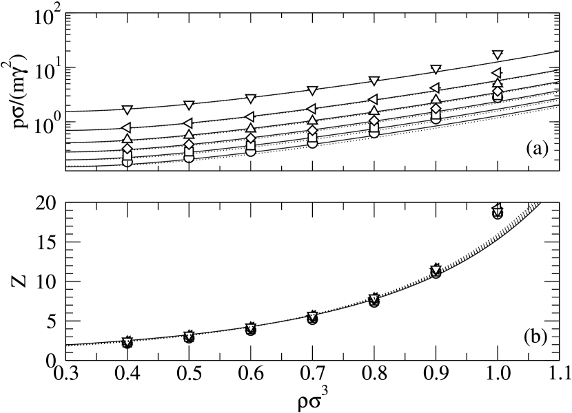
Figure 5: The (a) dimensionless pressure $p\sigma/(m\dot{\gamma}^{2})$ and (b) the compressibility factor $Z$ for inelastic hard-sphere systems with (i) $\alpha=0.4$ (circles), (ii) $\alpha=0.5$ (squares), (iii) $\alpha=0.6$ (diamonds), (iv) $\alpha=0.7$ (triangles-up), (v) $\alpha=0.8$ (triangles-left), and (vi) $\alpha=0.9$ (triangles-down). The uncertainty is smaller than the symbol size. The dotted lines are the suggested expressions of Ref. Montanero et al. (1999), and the solid lines are DSMC results. The solid line in (b) is the Carnahan-Starling equation of state for elastic hard sphere fluids, and the dotted lines are DSMC results for various $\alpha$.

The shear viscosity of a granular material is perhaps the most important design parameter in fast flows, quantifying the power lost per unit volume. The shear viscosity of the inelastic hard-sphere system was computed by two means. The first method is via the definition of the shear viscosity $\eta$ for simple Couette flow

$$\eta\equiv-\frac{\langle P_{xy}\rangle}{\dot{\gamma}}$$ (12)

An alternative method is to perform an energy balance. The work of shearing inputs energy into the system. Collisions between the inelastic spheres continuously dissipate kinetic energy. At steady-state, the average rate of energy input is equal to the average rate of energy dissipation Turner and Woodcock (1990):

$$\eta{\dot{\gamma}}^{2}V=-\langle\dot{E}\rangle$$ (13)

where $\langle\dot{E}\rangle$ is the average rate of kinetic energy dissipation. The rate of energy dissipation is directly related to the mean time between collisions $t_{\rm avg}$ for a sphere by

$$\langle\dot{E}\rangle=\frac{N}{2t_{\rm avg}}\langle\Delta{E}\rangle$$

where $N$ is the total number of spheres in the system, and $\langle\Delta{E}\rangle$ is the average amount of kinetic energy lost per collision.

The simulation results for the viscosity of sheared inelastic hard-sphere systems are summarized in Table 1. The upper entries are the values obtained from the stress tensor (see Eq. (11)), and the lower entries are the values obtained from the dissipation of kinetic energy (see Eq. (13)). For all the simulation runs, the two agree within the statistical uncertainties of the simulations. Figure 6a shows the dependence of the shear viscosity on the reduced density of the system, for various values of the coefficient of restitution. The viscosity increases with packing fraction and coefficient of restitution (remembering that the shear rate is equal to one). The theory of Montanero et al. captures the full Enskog behaviour and predicts the viscosity well. Enskog theory deviates at low values of $\alpha$ and high densities where the predictions for the temperature begin to deviate from the simulation results (see Fig. 2).

In addition to the shear viscosity, we also monitor the in-plane normal stress coefficient $\eta_{-}$ and the out-of-plane normal stress coefficient $\eta_{0}$, which are defined as Evans and Morris (1990)

$$\eta_{-} =-\frac{1}{2\dot{\gamma}}(\langle P_{xx}\rangle-\langle P_{yy}\rangle)$$

$$\eta_{0} =-\frac{1}{2\dot{\gamma}}\left[\langle P_{zz}\rangle-\frac{1}{2}(\langle P_{xx}\rangle+\langle P_{yy}\rangle)\right]$$

The in-plane normal stress coefficient is plotted in Fig. 6b, and the out-of-plane normal stress coefficient is plotted in Fig. 6c. The simulation values deviate significantly from the predictions of Enskog theory; however, this is unsurprising as the velocity dispersion predictions deviate significantly from the simulation results (see Fig. 3).

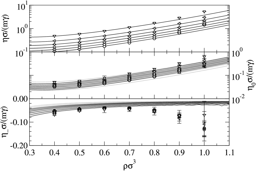
Figure 6: The viscosity for a homogeneously sheared inelastic-hard-sphere system with (i) $\alpha=0.4$ (circles), (ii) $\alpha=0.5$ (squares), (iii) $\alpha=0.6$ (diamonds), (iv) $\alpha=0.7$ (triangles-up), (v) $\alpha=0.8$ (triangles-left), and (vi) $\alpha=0.9$ (triangles-down). The dotted lines are the suggested expressions of Ref. Montanero et al. (1999), and the solid lines are DSMC results.

IV.3 Collision statistics

In this section, we examine the statistics of the collisions experienced by the spheres. The mean time between collision $t_{\rm{}avg}$ provides a characteristic time scale for the sheared inelastic hard sphere system. Figure 7 shows the variation of the mean time between collisions with the density of the system at various values of the coefficient of restitution. The time between collision decreases with a increasing density, which is expected; increasing the coefficient of restitution decreases the mean time between collision. The variation of $t_{\rm avg}$ with the coefficient of restitution is given in the inset of Fig. 7. At densities roughly below $\rho\sigma^{3}=0.6$, the mean time between collision decreases monotonically with increasing values of the coefficient of resitution. However, at higher densities, there is a maximum in $t_{\rm avg}$. The Enskog theory results describe the results qualitatively well for low density systems but fail at high densities.

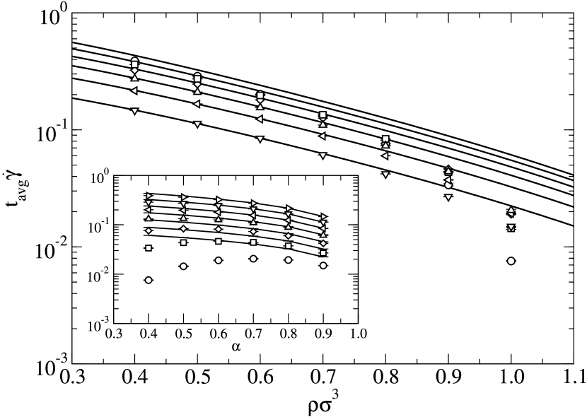
Figure 7: Mean time between collisions for sheared inelastic hard spheres with: (i) $\alpha=0.4$ (circles), (ii) $\alpha=0.5$ (squares), (iii) $\alpha=0.6$ (diamonds), (iv) $\alpha=0.7$ (triangles-up), (v) $\alpha=0.8$ (triangles-left), and (vi) $\alpha=0.9$ (triangles-down). Inset: variation of the mean time between collisions with the coefficient of restitution for (i) $\rho\sigma^{3}=1.0$ (circles), (ii) $\rho\sigma^{3}=0.9$ (squares), (iii) $\rho\sigma^{3}=0.8$ (diamonds), (iv) $\rho\sigma^{3}=0.7$ (triangles-up), (v) $\rho\sigma^{3}=0.6$ (triangles-left), (vi) $\rho\sigma^{3}=0.5$ (triangles-down), and (vii) $\rho\sigma^{3}=0.4$ (triangles-right). The solid lines are the DSMC simulation results.

For an elastic fluid, the velocities of different particles are, in general, uncorrelated. Consequently, the velocity statistics of the individual collisions can be determined exactly. On the other hand, the particle velocities in a driven granular system can be strongly correlated, and their on-collision statistics are not exactly known.

The distribution of the angle $\theta$ between the relative velocity and the relative position of two spheres on collision ($\cos\theta={\bf{}r}_{ij}\cdot{\bf{}v}_{ij}\,/\left|{\bf{}r}_{ij}\right|\left|{\bf{}v}_{ij}\right|$) is given in Fig. 8. The solid line denotes an isotropic collision distribution (as is the case for elastic, elastic-hard-sphere systems). The symbols are the simulation data for sheared inelastic hard spheres, and the solid line is the DSMC result for $\rho\sigma^{3}=0.9$ and $\alpha=0.4$. For weakly inelastic systems, the distribution of the collisional angle is close to that for the elastic hard-sphere system. As the inelasticity and density of the particles increases, however, there is a gradual increase of the frequency of “glancing” collisions (where $\cos\theta$ is near $0$) at the expense of more “head-on” collisions (where $\cos\theta$ is close to $-1$). This is in agreement with the two-dimensional shearing simulation of Tan and Goldhirsch Tan and Goldhirsch (1997) and Campbell and Brennen Campbell and Brennen (1985). The Enskog theory does not capture this effect, as the DSMC simulations only display a small increased bias towards glancing collisions even in the dense, highly inelastic system.

The increase in glancing collisions for strongly inelastic systems (see Fig. 8) results primarily from collisions between pairs of particles orientated in the $x$-$y$ plane. This occurs when the change of the streaming velocity over the diameter of a particle becomes significant in comparison to the average relative peculiar velocity Alam and Luding (2003). Particles separated in the $y$-plane then have a significantly increased relative velocity which increases their probability of collision. Both the DSMC and granular dynamics simulation results support this; however, DSMC does not exhibit the large increase in collisions with a very large collision angle.

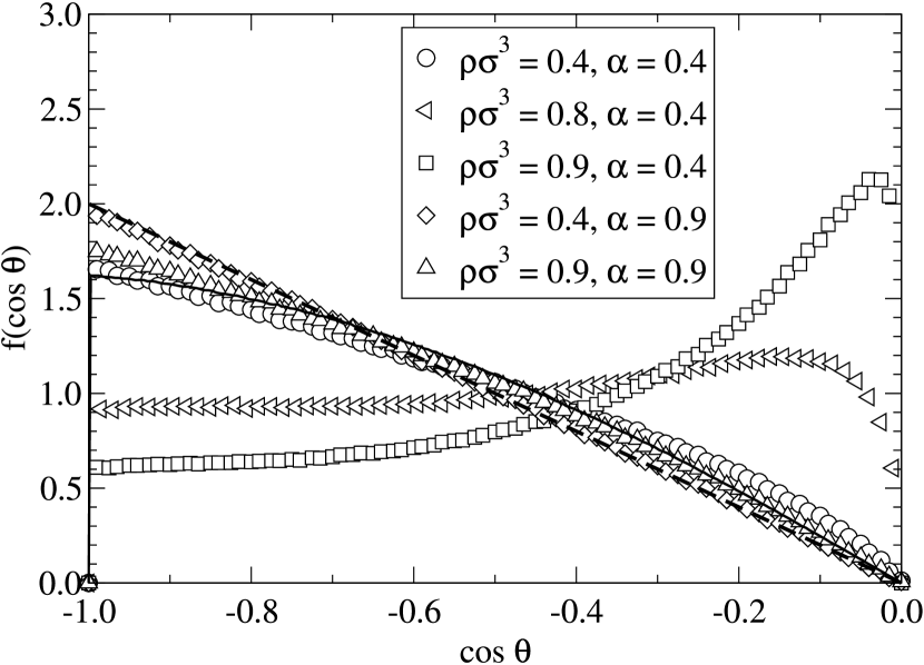
Figure 8: The distribution of collisional angles for (i) $\rho\sigma^{3}=0.4$ and $\alpha=0.4$ (circles), (ii) $\rho\sigma^{3}=0.8$ and $\alpha=0.4$ (triangles-left), (ii) $\rho\sigma^{3}=0.9$ and $\alpha=0.4$ (squares), (iii) $\rho\sigma^{3}=0.4$ and $\alpha=0.9$ (diamonds), and (iv) $\rho\sigma^{3}=0.9$ and $\alpha=0.9$ (triangles-up). The dashed line is for elastic hard spheres and the solid line is from a DSMC simulation of $\rho\sigma^{3}=0.9$ and $\alpha=0.4$.

In the inelastic hard sphere system, every collision results in a loss of kinetic energy. The simulation results for the distribution of the loss of kinetic energy on collision is given in Fig. 9. If the velocity distribution of the spheres were Gaussian (e.g., Maxwell-Boltzmann distribution), then the kinetic energy loss on collision would be distributed according to a Poisson distribution:

$$f(\Delta{E})=\frac{1}{\langle\Delta{E}\rangle}\exp\left(-\frac{\Delta{E}}{\langle\Delta{E}\rangle}\right)$$

This is given by the solid line in Fig. 9. At high values of $\alpha$, the distribution of the change of kinetic energy on collision is nearly exponential; for these systems, density does not significantly affect the results.

As $\alpha$ decreases, there is a greater frequency of collisions that result in a very slight loss of kinetic energy (i.e. the initial peak in Fig. 9). This corresponds to the increase in the glancing collisions in the systems. This enhancement of relatively elastic collisions is accompanied by an increase in collisions that result in large losses of kinetic energy (i.e. the long tail in Fig. 9). These result from “head-on” collisions, which occur between particles oriented primarily in the $x$-direction where the velocity dispersion is the greatest. While these “head-on” collisions occur less frequently than glancing collisions in the highly inelastic systems, they are more violent. Increasing the density enhances these effects.

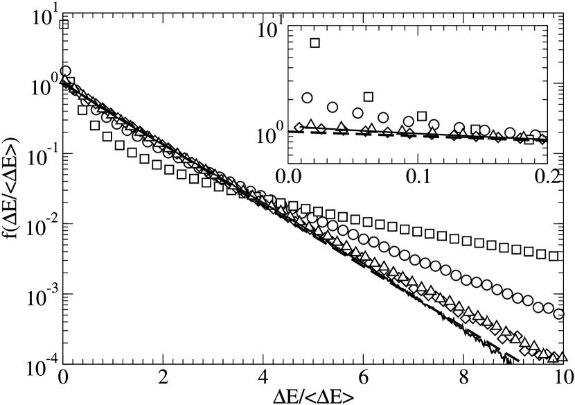
Figure 9: The change of kinetic energy on collision for sheared inelastic hard sphere systems with (i) $\rho\sigma^{3}=0.4$ and $\alpha=0.4$ (circles), (ii) $\rho\sigma^{3}=0.9$ and $\alpha=0.4$ (squares), (iii) $\rho\sigma^{3}=0.4$ and $\alpha=0.9$ (diamonds), and (iv) $\rho\sigma^{3}=0.9$ and $\alpha=0.9$ (triangles). The dashed line represents the kinetic energy loss on collision if the velocity were given by the Maxwell-Boltzmann distribution, and the solid line is from a DSMC simulation at $\rho\sigma^{3}=0.9$ and $\alpha=0.4$. The inset highlights the frequency of collisions that result in low energy losses.

Thus far, we have only studied the statistics of single collisions. One common assumption in many kinetic theories is that the individual collisions experienced by a particle are statistically independent. We now study the correlation between collisions by examining the time required for a particle to undergo a number of collisions. If the various collisions experienced by a particle can be considered to arrive at random times in an independent manner, then the time $t$ required for a particle to undergo $n$ collisions is given by a Poisson process. The probability density function $p_{n}(t)$ that a particle experiences $n$ collisions in a period of time $t$ is

$$p_{n}(t)=\frac{(t/t_{\rm avg})^{n-1}}{t_{\rm avg}\Gamma(n)}\exp\left(-\frac{t}{t_{\rm avg}}\right)$$ (14)

where $\Gamma(n)$ is the Gamma function. Deviations from this distribution are an indication of correlations between collisions. For elastic hard-sphere fluids, the Poisson process describes the collision time distribution fairly well, however, there are noticeable deviations, even at low densities, which increase with increasing density Lue (2005); Visco et al. (2008a, b)..

The collision time distributions for homogeneously sheared inelastic hard sphere systems are shown in Fig. 10. The solid lines denote the Poisson distribution, given by Eq. (14). At high values of the coefficient of restitution, the distributions are similar to those of elastic hard spheres and are fairly well described by a Poisson process. As the coefficient of restitution decreases, however, the simulation data deviate significantly from the Poisson process, indicating very strong correlations between collisions. Qualitatively, the deviations are similar to that observed for elastic hard sphere systems: there is an enhancement of very short and very long wait-times between collisions. However, these differences are much more pronounced for the inelastic hard sphere systems.

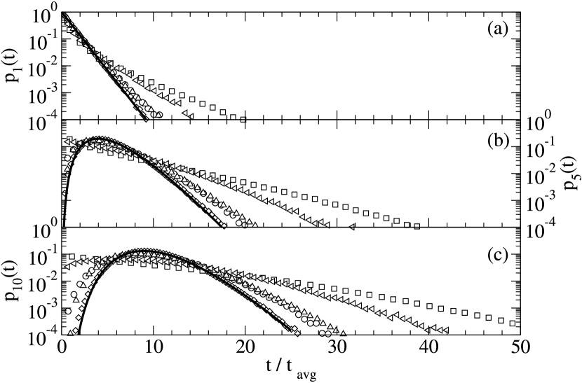
Figure 10: Distribution of time between (a) one collision, (b) five collisions, and (c) ten collisions in sheared inelastic hard spheres with (i) $\rho\sigma^{3}=0.4$ and $\alpha=0.4$ (circles), (ii) $\rho\sigma^{3}=0.9$ and $\alpha=0.4$ (squares), (iii) $\rho\sigma^{3}=0.4$ and $\alpha=0.9$ (diamonds), and (iv) $\rho\sigma^{3}=0.9$ and $\alpha=0.9$ (triangles). The solid line is for a Poisson process.

V Conclusions

We have performed non-equilibrium molecular dynamics simulations of sheared inelastic-hard-systems using the SLLOD algorithm combined with Lees-Edwards boundary conditions. In these simulations, care was taken to ensure that the systems remain homogeneous and the shear was uniform across the system. As a consequence, these simulations may prove a useful reference to compare with the predictions of kinetic theory.

DSMC simulations of the Enskog equation were performed to provide a solution to the kinetic theory without further approximation. These compared favorably with the simulation results except for dense, strongly inelastic systems. The velocity anisotropy effect can be very strong even in homogeneous systems, and kinetic theory solutions must take this into account in their approximations.

Results were presented for the velocity statistics of individual particles in the system. The velocity distributions were, in general, well described by an anisotropic Gaussian. Theories based on the anisotropic Gaussian and the full second moment balance (e.g., see Ref. Chou and Richman (1998)) are well suited to these systems. Sheared, inelastic-hard-sphere systems do not obey the equipartition theorem. Fluctuations of the velocity in the $x$-direction (the direction of shear) were greater than those in the $y$- and $z$-directions, which were both similar to each other. In addition, the granular temperature, which characterizes the overall fluctuation of the velocity, was observed to possess a minimum with respect to the density. This minimum becomes more pronounced as the coefficient of restitution of the spheres decreases.

The variation of the stress in the system was also examined. The compressibility factor of the sheared inelastic-hard-sphere system was quite similar to that of elastic hard spheres, as estimated by the Carnahan-Starling equation of state. The shear viscosity of the systems was computed in two different manners: from the average of the stress tensor and from the rate of dissipation of kinetic energy. The value of the viscosity from both these methods agree to within the statistical uncertainty of the simulations. The predictions of the Enskog equation and the kinetic theory of Montanero et al. Montanero et al. (1999) were in fairly good agreement with the simulation data. The in-plane and out-of-plane stress coefficients were also computed, but the kinetic theory predictions for these quantities were not as accurate.

Finally, the collision statistics of particles in the sheared inelastic hard sphere system were studied. The mean time between collision was found to decrease monotonically with increasing density; however, at fixed density, it displays a maximum at intermediate values of the coefficient of restitution. Examination of the collision time distributions indicated the presence of strong correlations between collisions. Including these correlations within a kinetic theory will be important in developing an accurate description of high density, sheared inelastic-hard-sphere systems.

Table 1: Dimensionless viscosity $\eta\sigma/(m\dot{\gamma})$ of sheared inelastic hard-sphere systems at various densities $\rho$ and coefficients of restitution $\alpha$. The upper value is determined from the stress tensor (see Eq. (11)), and the lower value is determined from the kinetic energy dissipation rate (see Eq. (13)). The value in brackets is the standard deviation over all of the runs.

	0.4	0.5	0.6	0.7	0.8	0.9
0.4	0.1054(0.0003)	0.1294(0.0004)	0.1625(0.0006)	0.2134(0.0005)	0.2970(0.0004)	0.480(0.002)
	0.1054(0.0003)	0.1294(0.0004)	0.1625(0.0006)	0.2134(0.0005)	0.2969(0.0004)	0.480(0.002)
0.5	0.1300(0.0003)	0.1582(0.0002)	0.1979(0.0007)	0.2585(0.0003)	0.361(0.001)	0.583(0.002)
	0.1300(0.0003)	0.1582(0.0002)	0.1979(0.0007)	0.2585(0.0003)	0.361(0.001)	0.583(0.001)
0.6	0.1722(0.0005)	0.2078(0.0003)	0.2606(0.0007)	0.3416(0.0009)	0.4785(0.0005)	0.779(0.006)
	0.1722(0.0005)	0.2078(0.0003)	0.2606(0.0007)	0.3417(0.0009)	0.4785(0.0007)	0.779(0.007)
0.7	0.2445(0.0004)	0.2909(0.0008)	0.364(0.001)	0.4801(0.0008)	0.677(0.002)	1.117(0.005)
	0.2446(0.0003)	0.2909(0.0008)	0.364(0.001)	0.4801(0.0009)	0.677(0.002)	1.117(0.005)
0.8	0.371(0.001)	0.4375(0.0002)	0.545(0.001)	0.716(0.003)	1.020(0.002)	1.722(0.008)
	0.371(0.001)	0.4375(0.0002)	0.545(0.001)	0.716(0.003)	1.020(0.002)	1.722(0.008)
0.9	0.643(0.007)	0.731(0.001)	0.885(0.002)	1.141(0.004)	1.64(0.01)	2.86(0.01)
	0.643(0.008)	0.731(0.002)	0.885(0.002)	1.141(0.004)	1.64(0.01)	2.856(0.010)
1.0	1.42(0.01)	1.52(0.02)	1.73(0.02)	2.15(0.03)	3.01(0.03)	5.30(0.04)
	1.42(0.01)	1.52(0.02)	1.73(0.02)	2.15(0.03)	3.01(0.04)	5.30(0.03)

References

- Campbell (1990) C. S. Campbell, Ann. Rev. Fluid Mech. 22, 57 (1990).
- Goldhirsch (2003) I. Goldhirsch, Annu. Rev. Fluid Mech. 35, 267 (2003).
- Campbell and Brennen (1985) C. S. Campbell and C. E. Brennen, J. Fluid Mech. 151, 167 (1985).
- Lutsko (2004a) J. F. Lutsko, Phys. Rev. E 70, 061101 (2004a).
- Lun et al. (1984) C. K. K. Lun, S. B. Savage, D. J. Jeffrey, and N. Chepurniy, J. Fluid Mech. 140, 223 (1984).
- Santos and Astillero (2005) A. Santos and A. Astillero, Phys. Rev E 72, 031308 (2005).
- van Beijeren and Ernst (1973) H. van Beijeren and M. H. Ernst, Physica 68, 437 (1973).
- Carnahan and Starling (1969) N. F. Carnahan and K. E. Starling, J. Chem. Phys. 51, 635 (1969).
- van Noije et al. (1998) T. P. C. van Noije, M. H. Ernst, and R. Brito, Physica A 251, 266 (1998).
- Sela and Goldhirsch (1998) N. Sela and I. Goldhirsch, J. Fluid Mech. 361, 41 (1998), URL http://journals.cambridge.org/action/displayAbstract?aid=1486%5.
- Lun (1991) C. K. K. Lun, J. Fluid Mech. 233, 539 (1991).
- Goldhirsch (2008) I. Goldhirsch, Powder Tech. 182, 130 (2008).
- Jenkins and Richman (1988) J. T. Jenkins and M. W. Richman, J. Fluid Mech. 192, 313 (1988), URL http://journals.cambridge.org/production/action/cjoGetFulltex%t?fulltextid=394683.
- Jenkins and Richman (1985) J. T. Jenkins and M. W. Richman, Physics Of Fluids 28, 3485 (1985).
- Montanero et al. (1999) J. M. Montanero, V. Garzo, A. Santos, and J. J. Brey, J. Fluid Mech. 389, 391 (1999), URL http://journals.cambridge.org/action/displayAbstract?aid=1525%3.
- Santos et al. (1998) A. Santos, J. M. Montanero, J. W. Dufty, and J. J. Brey, Phys. Rev. E 57, 1644 (1998).
- Brey et al. (1999) J. J. Brey, J. W. Dufty, and A. Santos, J. Stat. Phys. 97, 281 (1999).
- Bird (1994) G. A. Bird, Molecular gas dynamics and the direct simulation of gas flows (Oxford Science, 1994).
- Hopkins and Shen (1992) M. A. Hopkins and H. H. Shen, J. Fluid Mech. 244, 477 (1992).
- Montanero and Santos (1997) J. M. Montanero and A. Santos, Phys. Fluids 9, 2057 (1997).
- Alam and Luding (2003) M. Alam and S. Luding, Phys. Fluids 15, 2298 (2003).
- M. and S. (2005) A. M. and L. S., Phys. Fluids 17, 063303 (2005).
- Campbell (1989) C. Campbell, J. Fluid Mech. 203, 449 (1989).
- Herbst et al. (2004) O. Herbst, P. Müller, M. Otto, and A. Zippelius, Phys. Rev. E 70, 051313 (2004).
- Herrmann et al. (2001) H. J. Herrmann, S. Luding, and R. Cafiero, Physica A 295, 93 (2001).
- Conway and Glasser (2004) S. L. Conway and B. J. Glasser, Phys. Fluids 16, 509 (2004).
- Alam et al. (2005) M. Alam, V. H. Arakeri, P. R. Nott, J. D. Goddard, and H. J. Herrman, J. Fluid. Mech. 523, 277 (2005).
- Lees and Edwards (1972) A. W. Lees and S. F. Edwards, J. Phys. C 5, 1921 (1972).
- Walton and Braun (1986) O. R. Walton and R. L. Braun, J. Rheol. 30, 949 (1986).
- Hopkins and Louge (1991) M. A. Hopkins and M. Y. Louge, Phys. Fluids A 3, 47 (1991).
- Goldhirsch and Tan (1996) I. Goldhirsch and M.-L. Tan, Phys. Fluids 8, 1752 (1996).
- Tan and Goldhirsch (1997) M.-L. Tan and I. Goldhirsch, Phys. Fluids 9, 856 (1997).
- Lutsko (2004b) J. F. Lutsko (2004b), eprint arXiv:cond-mat/0403551v1, URL http://arxiv.org/abs/cond-mat/0403551.
- Losert et al. (1999) W. Losert, D. Cooper, J. Delour, A. Kudrolli, and J. Gollub, Chaos 9, 682 (1999), URL http://link.aip.org/link/?CHAOEH/9/682/1.
- Montanero et al. (2006) J. M. Montanero, V. Garzó, M. Alam, and S. Luding, Gran. Matt. 8, 103 (2006).
- Evans and Morris (1990) D. J. Evans and G. P. Morris, Statistical Mechanics of Nonequilibrium Liquids (Academic Press, London, 1990).
- Petravic and Jepps (2003) J. Petravic and O. G. Jepps, Phys. Rev. E 67, 021105 (2003).
- McNamara and Falcon (2003) S. McNamara and E. Falcon, in Granular Gas Dynamics (Springer, 2003), pp. 347–366.
- McNamara and Young (1996) S. McNamara and W. R. Young, Phys. Rev. E 53, 5089 (1996).
- Alam and Hrenya (2001) M. Alam and C. Hrenya, Phys. Rev. E 63, 061308 (2001).
- Alder and Wainwright (1959) B. J. Alder and T. E. Wainwright, J. Chem. Phys. 31, 459 (1959).
- Bannerman and Lue (2008) M. Bannerman and L. Lue, Dynamics of discrete objects (dynamo), World Wide Web (2008), URL http://www.marcusbannerman.co.uk/dynamo.
- Dufty et al. (1997) J. W. Dufty, J. J. Brey, and A. Santos, Physica A 240, 212 (1997).
- Campbell (2002) C. S. Campbell, J. Fluid Mech. 465, 261 (2002).
- Knight and Woodcock (1996) T. A. Knight and L. V. Woodcock, J. Phys. A 29, 4365 (1996).
- Olafsen and Urbach (1999) J. S. Olafsen and J. S. Urbach, Phys. Rev. E 60, R2468 (1999).
- Rouyer and Menon (2000) F. Rouyer and N. Menon, Phys. Rev. Lett. 85, 3676 (2000).
- Alder et al. (1970) B. J. Alder, D. M. Gass, and T. E. Wainwright, J. Chem. Phys. 53, 3813 (1970).
- Turner and Woodcock (1990) M. Turner and L. Woodcock, Powder Technology 60, 47 (1990).
- Lue (2005) L. Lue, J. Chem. Phys. 122, 044513 (2005).
- Visco et al. (2008a) P. Visco, F. van Wijland, and E. Trizac, J. Phys. Chem. B 112, 5412 (2008a).
- Visco et al. (2008b) P. Visco, F. van Wijland, and E. Trizac, Phys. Rev. E 77, 041117 (2008b).
- Chou and Richman (1998) C.-S. Chou and M. W. Richman, Physica A: Statistical and Theoretical Physics 259, 430 (1998), ISSN 0378-4371.