Analysis of the electric field gradient in the perovskites SrTiO₃ and BaTiO₃: density functional and model calculations

Abstract

We analyze recent measurements [R. Blinc, V. V. Laguta, B. Zalar, M. Itoh and H. Krakauer, J. Phys. : Condens. Matter 20, 085204 (2008)] of the electric field gradient on the oxygen site in the perovskites SrTiO₃ and BaTiO₃, which revealed, in agreement with calculations, a large difference in the EFG for these two compounds. In order to analyze the origin of this difference, we have performed density functional electronic structure calculations within the local-orbital scheme FPLO. Our analysis yields the counter-intuitive behavior that the EFG increases upon lattice expansion. Applying the standard model for perovskites, the effective two-level $p$-$d$ Hamiltonian, can not explain the observed behavior. In order to describe the EFG dependence correctly, a model beyond this usually sufficient $p$-$d$ Hamiltonian is needed. We demonstrate that the counter-intuitive increase of the EFG upon lattice expansion can be explained by a $s$-$p$-$d$ model, containing the contribution of the oxygen 2$s$ states to the crystal field on the Ti site. The proposed model extension is of general relevance for all related transition metal oxides with similar crystal structure.

I Introduction

Perovskite compounds $AB$O₃, with $A$ being an alkali, alkaline earth or rare earth metal and $B$ a transition metal element, attract much attention because of their importance both for fundamental science and for technological applications LinesGlass . Although the high-temperature cubic phase has a very simple crystal structure, this does not prevent these compounds to exhibit a large variety of physical properties rendering the perovskites to model compounds for studies of a large variety of different physical phenomena. Within the perovskite family, we find superconductivity, e.g. in K_xBa_1-xBiO₃ Matth88 , giant magnetoresistance, e.g. in LaMnO₃ Moritomo96 , orbital ordering, e.g. in YTiO₃ Ishihara02 and ferroelectricity, e.g. in BaTiO₃ Cohen92 . The latter phenomena are of large interest because of technological applications.

The compounds SrTiO₃ (STO) and BaTiO₃ (BTO) are usually considered to be isovalent. The valence and conduction bands of the two perovskites are formed by $p$-states of oxygen and $d$-states of titanium. In the high-temperature cubic phase, the Ti and O sub-lattices have the identical geometry for STO and BTO, the lattice parameters being $a$=3.8996 Å STO and $a$=4.009 Å LinesGlass respectively. As the temperature lowers, both compounds experience a softening of an optical phonon mode, which corresponds to Ti motion towards the oxygen LinesGlass . BTO exhibits a succession of phase transitions, from the high-temperature cubic perovskite phase to ferroelectric structures with tetragonal, orthorhombic and rhombohedral symmetry LinesGlass . In contrast, STO behaves as an incipient ferroelectric in the sense that it remains paraelectric down to the lowest temperatures, exhibiting nevertheless a very large static dielectric response. It undergoes an antiferrodistortive phase transition at 105 K to a tetragonal ($I4/mcm$) phase, but this transition is of non-polar character and has little influence on the dielectric propertiesSai2000 .

The first determination of the ¹⁷O electric field gradient (EFG) on the oxygen site in perovskites was recently reported for STO and BTO Blinc08 together with first-principle calculations using the linearized augmented plane wave (LAPW) method was used. The most striking feature in the experimental and theoretical data is the large difference of the EFGs between the two compounds. The calculational investigation of Blinc et al. concluded, that the magnitude of the EFG of ¹⁷O in BTO is larger than the EFG of ¹⁷O in STO due to two effects: $(i)$ larger lattice parameters in BTO compared to STO and $(ii)$ a larger ionic radius of Ba compared to Sr. While the experimental determination (NMR) can not provide the sign of the EFG, the LAPW calculation yielded a negative EFG. A negative EFG corresponds to a prolate electron density, which implies the importance of covalence effects.

In order to elucidate the origin of the sign of and the different contributions to the EFG, we have performed first-principle calculations using a local orbital code (FPLO FPLO ) that is especially suited to address these questions due to its representation of the potential and the density allowing easy decomposition. The calculational details of our investigation are given in Sec. II, and the obtained results are presented in Sec. III. These results can not be explained by intuitive models, which are also described in this section. Therefore, a more complex microscopic model Hamiltonian is introduced in Sec. IV. Using the properties of this $p$-$d$ like Hamiltonian, an agreement with the obtained experimental and theoretical results and a deeper, microscopically based understanding is obtained.

II Calculation methods

The electronic band structure calculations were performed with the full-potential local-orbital minimum basis code FPLO (version 5.00-19) FPLO within the local density approximation. In the scalar relativistic calculations the exchange and correlation potential of Perdew and Wang PW was employed. As basis sets Ba (4d5s5p/6s6p5d+4f7s7p), Sr (4s4p/5s5p4d+6s6p), Ti (3s3p3d/4s4p4d+5s5p) and O (2s2p3d+3s3p) were chosen for semicore/valence+polarization states. The high lying states improve the completeness of the basis which is especially important for accurate EFG calculations. The lower lying states were treated fully relativistic as core states. A well converged $k$-mesh of 455 $k$-points was used in the irreducible part of the Brillouin zone.

III FPLO analysis results

	SrTiO3	BaTiO3	Ref.
$|V_{zz}^{exp}|$	1.62	2.46	Ref. Blinc08,
$V_{zz}^{cal}$	-1.00	-2.35	Ref. Blinc08,
$V_{zz}^{cal}$	1.00	2.44	Eq. (29)
$V_{zz}^{on}$	-0.21	1.39	Eq. (30)
$V_{zz}^{off}$	1.21	1.05	Eq. (31)
$V_{zz,pp}^{on,net}$	96%	107%	Eq. (34)

Table 1: The experimental and calculated values of the EFG (in 10²¹ V/m²) on the oxygen site in the cubic phase of the two perovskites. The last four lines refer to equations given in the appendix.

In FPLO, the EFG on a nucleus at a given lattice site may be represented as the sum of two contributions: An on-site contribution $V_{zz}^{on}$ (see Eq.(30)), which comes from the on-site contribution of the electron density of the given lattice site, and a second term, the off-site contribution $V_{zz}^{off}$ (see Eq.(31)), which results from the potential of all other atoms (see App. A). The on-site contribution $V_{zz}^{on}$ can be analyzed further. It can be split up in $p$-$p$, $s$-$d$ and $d$-$d$ contributions (see App. B).

The on- and off-site contributions as well as their sum and the dominating $p$-$p$ contribution (see Eq. (34)) are shown in Tab. 1. Whereas the total EFG for ¹⁷O in BTO agrees well with the experiment (1 % deviation), the total EFG for ¹⁷O in STO is in discrepancy with the experiment (38 % deviation), see Tab. 1. Compared to the EFGs calculated with the LAPW code in Ref. Blinc08, , we obtain almost the same absolute value of $V_{zz}$ but the opposite sign, see Tab. 1. Our calculated EFGs as a function of the lattice parameter $a$ for both compounds reveal the same tendency as observed in Ref. Blinc08, : The absolute value of the EFG increases under the lattice expansion (see Fig. 1). From Fig. 1 we also conclude that the EFG of BTO is not only larger than the EFG of STO due to larger lattice parameters (“lattice effect”), but also due to an “cation effect”, which is responsible for the remaining difference. This lattice effect is demonstrated by the shift between the two EFG curves in Fig. 1.

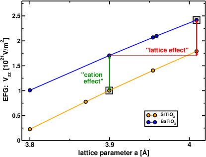
Figure 1: Calculated $V_{zz}$ in dependence of the lattice parameter $a$. $V_{zz}$ for the experimental lattice parameter is marked by a shaded square. The “cation” and “lattice effect”, which are responsible for the difference in $V_{zz}$ for these two compounds are indicated by the red and black arrow, respectively. Inset: The anisotropy count $\Delta p$ (see text) in dependence of the lattice parameter $a$.

The increase of the (absolute value of the) EFG upon lattice expansion is rather counter-intuitive. In the traditional approach, the spherically symmetric electronic shell of an ion is perturbed by the potential of the external (point) charges of the solid. As a result, the total EFG on the ion nucleus is caused by the EFG of the external potential, and is roughly proportional to it. It is clear that this approach predicts the opposite tendency: The strength of the external potential is inversely proportional to the lattice constant and thus the (absolute value of the) EFG should diminish under the lattice expansion. The failure of this approach to describe the observed behavior of the EFG indicates that a fully ionic description of the perovskites is inappropriate.

In an alternative approach, the electronic shell of the atom is disturbed by the hybridization of the wave functions with the states of the surrounding atoms. The hybridization results in the asymmetry of the electronic cloud of the atom and the EFG on its nucleus. Apparently, this covalent approach predicts the same tendency as the ionic one: It is usually believed that the hybridization diminishes with the increase of the bond length. In both approaches we may say: When expanding the lattice, we diminish its influence on the atom, and the electronic shell should become closer to that of the free atom. Hence, we come to the conclusion: The (absolute value of the) EFG should diminish under the lattice expansion, which is opposite to the experimental observation and the results of both first-principle calculations. We will tackle this problem in detail in Sec. IV.

Another problem it the different sign of the EFG obtained from the two different band structure codes. If the sign of the EFG is taken into account, the slope in our graph (Fig. 1) is opposite to the slope in the graph obtained with the LAPW code (Fig. 5 in Ref. Blinc08, ). Since the NMR experiment is not sensitive to the sign of the EFG, we will investigate the influence of the lattice expansion on the different contributions to the EFG to get more insight in this issue.

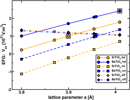
Figure 2: The on-site $V_{zz}^{on}$, off-site $V_{zz}^{off}$ and total EFG as a function of the lattice parameter $a$. The grey shaded squares mark the experimental lattice parameter for $V_{zz}$.

Our calculations show that both the on-site and the off-site contribution to the EFG have comparable values for the perovskite lattice, see Tab. 1 and Fig. 2. In Fig. 2, the two contributions, $V_{zz}^{on}$ (dashed line) and $V_{zz}^{off}$ (dash-point line) and the total EFG (full line) are shown. Whereas the off-site EFG decreases only slightly upon lattice expansion, the on-site EFG increases strongly with increasing lattice parameters, resulting in the significant increase of the total EFG. We also observe that the off-site EFG is almost identical for these two structures, which is in line with the observed weak dependence of $V_{zz}^{off}$ on the lattice parameters.

The on-site EFG is mainly caused by electrons with $p$ character, see table 1. Therefore, we will investigate the corresponding anisotropy count $\Delta p$ Blaha88 . In the perovskite structure $AB$O₃, the oxygen site has axial symmetry, and the $z$-axis is directed along the $B$-O bond. Thus, the anisotropy count is the difference between the population of the oxygen 2$p$ $\sigma$- (corresponds to $p_{z})$ and $\pi$- (corresponds to $p_{x,y})$ orbitals. In the inset of Fig. 1 we see that the anisotropy count $\Delta p$ increases with the lattice expansion. This is in agreement with the increasing on-site EFG. If we focus on BTO, where the experimental and calculated (for the experimental lattice parameter $a=4.009$ Å) value for the EFG agree very well, we see that this positive $V_{zz}$ corresponds to a positive $\Delta p$. That means the $p$ electron density (responsible for the EFG) has an oblate shape, since more electrons are occupying the $p_{x,y}$-orbitals than the $p_{z}$-orbital, which is in agreement with the positive sign of the EFG.

After concluding that the sign of $V_{zz}$ for ¹⁷O for both STO and BTO should be positive, we come back to the counter intuitive behavior of the increasing EFG upon lattice expansion. Fig. 3 reveals that the increase of $\Delta p$ under lattice expansion, which is responsible for the increasing EFG upon lattice expansion, is due to an increasing occupation of $pi$- (corresponds to $p_{x,y})$ and an decreasing population of $\sigma$- (corresponds to $p_{z})$ orbitals.

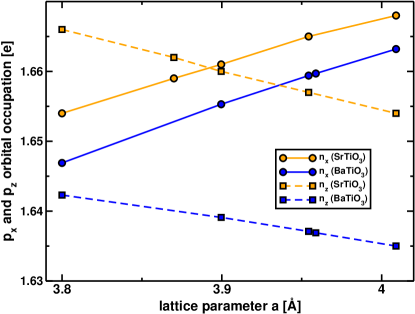
Figure 3: Occupation of $p_{x}$ and $p_{z}$ states in dependence of the lattice parameter $a$.

IV Discussion

In order to understand this anomalous behavior of the $\sigma$-orbital, we will analyze the main features of the electronic structure of perovskites. Detailed band structure studies of perovskite compounds were performed by Mattheiss Matth69 ; Matth72 ; Matth70 , who also proposed a first tight-binding fit for the band dispersions. Wolfram et al. Wolfram72 ; Wolfram73 ; Wolfram82 (cf. also Ref. Pros87, ) developed a very simple model (Wolfram and Ellialtioglu, WE) for the valence and conduction bands, which reflects their basic properties. The WE model includes the $d$-orbitals of the $B$ ion and the $p$-orbitals of the oxygen. Wolfram et al. pointed a quasi-two-dimensional character of the bands out, which is due to the symmetry of the orbitals. If one retains only nearest neighbor hoppings, the total $14\times 14$ Hamiltonian matrix (five $d$-orbitals and 9 $p$-orbitals) acquires block-diagonal form at every value of the momentum. The three $3\times 3$ matrices describe the $\pi_{ij}$-bands ($ij=xy,yz,xz$). Every $d_{ij}$-orbital of the $t_{2g}$ symmetry couples with its own combination of oxygen $2p$ $\pi$-orbitals, which lie in the same plane perpendicular to the bond direction. They form a pair of bonding and anti-bonding states. The remaining combination of the $2p$ $\pi$-orbitals in the same plane forms the non-bonding band. Wolfram et al. call this group of bands $\pi$-bands. The states described by the $5\times 5$ block matrix are called $\sigma$-bands, since they are formed by oxygen $2p$ $\sigma$-orbitals, which are coupled with the $e_{g}$ ($d_{x^{2}-y^{2}}$ and $d_{z^{2}}$) orbitals of the B ion. This matrix decouples into one non-bonding band and two pairs of bonding and anti-bonding bands.

Fig. 4 shows the calculated band structure for STO for two different lattice parameters $a$. The features mentioned above are clearly seen (cf. Fig. 2 of Ref. Wolfram82, ). The anti-bonding $\pi_{ij}$-bands are situated between 2 and 4 eV, where the $\pi_{yz}$-band is almost dispersionless in the direction $\Gamma\rightarrow X$. This manifests the quasi-two-dimensional character of the bands. The bands originating from the $d$ $e_{g}$-orbitals are in the range from 4 to 8 eV, where the band expressing $d_{z^{2}}$ character is dispersionless along the $\Gamma\rightarrow X$ direction. The valence band has a more complex character due to additional mixing from the direct $p-p$ hopping. This is neglected in the simple version of the WE model. Nevertheless, we see that the non-bonding bands lie on top of the valence band and have a much smaller dispersion than the bonding bands, which lie below $-1$ eV ($\pi_{ij}$) and below $-3$ eV ($\sigma$-bands). The latter have a larger dispersion due to much larger $d-p$ hoppings.

Although the Kohn Sham theory is not good for excitation spectra, or obtaining the correct energy gap, it yields reliable occupation numbers, on-site energies and transfer integrals, especially in the absence of strong correlations. Therefore, we can use our LDA band structure to obtain reliable parameters as input for further treatment using model Hamiltonians.

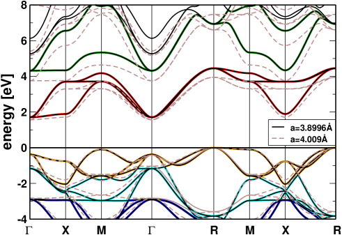
Figure 4: SrTiO₃: band structure for two different lattice parameters $a=3.8996$ Å (black/colored full lines) and $a=4.009$ Å (brown dashed lines). The different band characters are given by different colors: blue (bonding, $\sigma$), cyan (bonding, $\pi$), orange (non-bonding), red (anti-bonding, $\pi_{ij}$) and green (anti-bonding, $d_{eg}$), see text. Since it is not easy to interpret the valence band, the colors in the valence band are only approximate.

In the following, we explore within the WE model how the occupation numbers and the resulting anisotropy count for the $p$-orbitals depend on the lattice parameters. In dielectric compounds like STO and BTO, the bonding and non-bonding states are fully occupied. Contrary to the non-bonding bands, which have almost pure $p$-character, the bonding and anti-bonding bands are mixed $p$-$d$-bands. The population of the $p$-orbitals is given by the sum of the occupation numbers of the non-bonding and the bonding bands, whereof the latter are lattice parameter dependent.

Every pair of bonding and anti-bonding states is described by an effective two-level model Wolfram73

$$\hat{H}_{m} = \Delta_{m}\left(\left|d,\mathbf{k}\right\rangle\left\langle d,\mathbf{k}\right|-\left|p,\mathbf{k}\right\rangle\left\langle p,\mathbf{k}\right|\right)$$ (1)

$$+V_{m}f_{m\mathbf{k}}\left(\left|d,\mathbf{k}\right\rangle\left\langle p,\mathbf{k}\right|+\left|p,\mathbf{k}\right\rangle\left\langle d,\mathbf{k}\right|\right).$$

Here, $m$ describes the character of the band $m=\pi,\sigma$ and $f_{m\mathbf{k}}$ is a dimensionless function, which depends on the dimensionless variable $\mathbf{k}a$ (note that $\mathbf{k}$ is measured in units of $\pi/a$, so neither $\mathbf{k}a$ nor $f_{m\mathbf{k}}$ depends on $a$). The state mixing is defined by the interplay of the on-site energy difference $\Delta_{m}$ and the transfer integral $V_{m}$, which determines the bandwidth of the corresponding band. The eigenstates of the Hamiltonian Eq. (1) have the form

$$\left|\mathbf{k},\nu\right\rangle=c_{d\mathbf{k}\nu}\left|d,\mathbf{k}\right\rangle+c_{p\mathbf{k}\nu}\left|p,\mathbf{k}\right\rangle,$$ (2)

and for the $p$-states, the following energies and occupation numbers are obtained

$$E_{\mathbf{k}m\nu} = \nu\sqrt{\Delta_{m}^{2}+V_{m}^{2}\left(f_{m\mathbf{k}}\right)^{2}},\ \nu=\pm 1$$ (3)

$$n_{p\mathbf{k}m\nu} \equiv 2\left|c_{p\mathbf{k}\nu}\right|^{2}=1-\Delta_{m}/E_{\mathbf{k}\nu}.$$ (4)

$$n_{d\mathbf{k}m\nu} \equiv 2\left|c_{d\mathbf{k}\nu}\right|^{2}=2\left(1-\left|c_{p\mathbf{k}\nu}\right|^{2}\right)=1+\frac{\Delta_{m}}{E_{\mathbf{k}\nu}}$$ (5)

Here, $\nu=+1$ describes the anti-bonding and $\nu=-1$ describes the bonding band. In this two-level system, two asymptotic behaviors are possible. First, $\Delta_{m}/V_{m}\rightarrow\infty$, which yields for the occupation numbers of the bonding bands $n_{p\mathbf{k}m,-1}\rightarrow 2$ and $n_{d\mathbf{k}m,-1}\rightarrow 0$. In this case, both electrons are in the $p$-state of the ligand ion and $d$-states are empty, called the ionic limit. Second, $\Delta_{m}/V_{m}\rightarrow 0$, which yields for the occupation numbers $n_{p\mathbf{k}m,-1}\rightarrow 1$ and $n_{d\mathbf{k}m,-1}\rightarrow 1$. In this case, the electrons are equally shared by the $p$-, and $d$-states. This is the covalent limit. From the trends in Fig. 3, we observe that while the population of the $p_{\pi}$-orbitals increases, the population of the $p_{\sigma}$-orbitals decreases. This means the Ti-O $\pi$-bond gets more ionic under lattice expansion (as expected) whereas the Ti-O $\sigma$-bond gets more covalent, which we will try to explain with this model.

The parameters of this model can be extracted from the band energies at symmetry points of the Brillouin zone in Fig. 4 (see the App. C for more details).

For example, the on-site energies $\Delta_{m}$ can be obtained from the $\Gamma$ point, since due to symmetry, the $d-p$ mixing vanishes at this point and the band states acquire a pure $d$ or $p$ character. For $a=3.8996$ Å we have for STO $E_{d_{t2g}}\approx 1.7$ eV, $E_{d_{eg}}\approx 4.3$ eV, $E_{p}\approx-1.2$ eV. This yields (using Eq. (45) and Eq. (44)) $2\Delta_{\pi}=E_{d_{t2g}}-E_{p}\approx 2.9$ eV and $2\Delta_{\sigma}=E_{d_{eg}}-E_{p}\approx 5.5$ eV.

From these values and the $f_{mk}$ as given in Refs. Wolfram73, ; Wolfram82, we obtain the Slater-Koster hopping parameters $V_{\sigma}\approx 2.1$ eV Eq. (47), $V_{\pi}=V_{pd\pi}\approx 1.6$ eV Eq. (46) and $V_{pd\sigma}\approx 2.7$ eV Eq. (49).

Since the occupation numbers of the non-bonding bands do not depend on the lattice and the anti-bonding bands ($\nu=+1$) are not occupied, we consider the bonding bands ($\nu=-1$) only. The contributions from the bonding bands to the population of the $p_{m}$ orbitals $n_{p_{m}}$ are obtained by a sum over the Brillouin zone. In order to analyze the occupation in dependence of the lattice expansion, we need the derivative of the occupation number with respect to the lattice parameter $a$. From Eq. (4) we obtain for the derivative (denoted by $\prime$)

$$n_{p\mathbf{k}m,-1}^{\prime}=\frac{V_{m}^{2}\left(f_{m\mathbf{k}}\right)^{2}\Delta_{m}}{\left(\sqrt{\Delta_{m}^{2}+V_{m}^{2}\left(f_{m\mathbf{k}}\right)^{2}}\right)^{3}}\left(\frac{\Delta_{m}^{\prime}}{\Delta_{m}}-\frac{V_{m}^{\prime}}{V_{m}}\right).$$ (6)

The derivative of $n_{p_{m}}$ is proportional to

$$n_{p_{m}}^{\prime}\propto\left(\frac{\Delta_{m}^{\prime}}{\Delta_{m}}-\frac{V_{m}^{\prime}}{V_{m}}\right).$$ (7)

Fig. 3 shows that $n_{p_{m}}^{\prime}$ has a different behavior for $m=\sigma$ ($n_{p_{\sigma}}^{\prime}$ is negative) and $m=\pi$ ($n_{p_{\pi}}^{\prime}$ is positive). Thus, within the WE model, the observed increase of the EFG, which is due to the decreasing occupation of the ${p_{\sigma}}$-orbitals would yield

$$-\frac{V_{\sigma}^{\prime}}{V_{\sigma}}<-\frac{\Delta_{\sigma}^{\prime}}{\Delta_{\sigma}}.$$ (8)

Both $\Delta_{\sigma}$ and $V_{\sigma}$ decrease upon lattice expansion: Fig. 4 shows that the energies at the $\Gamma$-point $E_{d_{eg}}$ and $E_{d_{t2g}}$ and the bandwidths are smaller for the larger lattice parameter $a=4.009$ Å, than for the smaller lattice parameter $a=3.8996$ Å. A commonly accepted estimate Harrison for the dependence of hopping integrals on $a$ is $V_{\sigma}\propto a^{-\alpha}$ with $\alpha$ between 3.5 and 4 (from the LDA band structure, we obtain $\alpha=3.5\pm 0.5$). This gives

$$-a\frac{V_{\sigma}^{\prime}}{V_{\sigma}}=\alpha\geq 3.$$ (9)

$\Delta_{\sigma}$ is the difference in energy of the atomic levels corrected by the crystal field (CF) $\Delta_{\sigma}=\varepsilon_{d}-\varepsilon_{p}+\delta_{CF,\sigma}$. The crystal field consists of two contributions crystalField : A (dominating) electrostatic contribution, which is the difference of the Madelung potentials of Ti and O, hence $\delta_{CF,el}\propto a^{-1}$, and a hybridization contribution, which, in our case (octahedral coordination), contains a large and strongly $a$-dependent contribution for $m=\sigma$ from the semi-core $s$-states of the ligand. Indeed, (cf. Fig. 4) the change due to the increasing lattice parameter $a$ is much larger for $\Delta_{\sigma}$ than for $\Delta_{\pi}$. The main electrostatic contribution, which implies $\delta_{CF,el}\propto a^{-1}$, leads to

$$-a\frac{\Delta_{\sigma}^{\prime}}{\Delta_{\sigma}}=\frac{\delta_{CF,el}}{\Delta_{\sigma}}.$$

Since $\varepsilon_{d}-\varepsilon_{p}+\delta_{CF,el}>\delta_{CF,el}$ is $\delta_{CF,el}/\Delta_{\sigma}<1$ and therefore

$$-a\frac{\Delta_{\sigma}^{\prime}}{\Delta_{\sigma}}<1.$$ (10)

Combining the estimates from Eq. (9) and Eq. (10), we get

$$-a\frac{\Delta_{\sigma}^{\prime}}{\Delta_{\sigma}}<1<3\leq-a\frac{V_{\sigma}^{\prime}}{V_{\sigma}}.$$ (11)

This is in contradiction to the inequality (8), leading to the conclusion that the WE model, though consistent with the intuitive expectations (see Sec. III) is unable to predict the observed behavior of the $\sigma$-orbital occupation in Fig. 3.

A possible reason for the failure of the WE model is that according to Ref. Matth70, , a large contribution to the CF comes from the oxygen 2$s$-orbitals, which lie almost 18 eV below the Ti 3$d$ level, $\Delta_{sd}=17.9$ eV, but have a large matrix element $V_{sd\sigma}=3.0$ eV with the $e_{g}$ orbitals. This suggests to extend the WE model taking into account the oxygen 2$s$-states in order to explain the increasing EFG upon lattice expansion. This is Harrison’s model, where $V_{sd\sigma}$ is obtained from Eq. (48)

$$\Gamma_{12}=\frac{\varepsilon_{s}+\varepsilon_{d}}{2}\pm\sqrt{(\frac{\varepsilon_{s}-\varepsilon_{d}}{2})^{2}+6V_{sd\sigma}^{2}},$$

with $\varepsilon_{s}=-16.2$ eV, $\varepsilon_{d}=1.7$ eV and $\Gamma_{12}=4.3$ taken from the band structure.

Taking the $s$-orbitals into account, $V_{\sigma}$ in the inequality (8) is replaced by $V_{sd\sigma}$. Harrison Harrison argues that the $a$ dependence of $V_{sd\sigma}$ is similar to the a dependence of $V_{pd\sigma}$. This suggestion is confirmed by our LDA calculations. Thus, we obtain

$$\frac{V_{sd\sigma}\prime}{V_{sd\sigma}}=-\frac{\alpha}{a}.$$ (12)

On the right hand side we have the on-site energy difference, which is given by $\Delta_{\sigma}\approx\Delta_{\pi}+3V_{sd\sigma}^{2}/\Delta_{sd}$, cf. Eq. (52). The derivative of this expression is

$$\Delta_{\sigma}^{\prime}\approx\frac{6}{\Delta_{sd}}V_{sd\sigma}V_{sd\sigma}^{\prime}.$$ (13)

Note, that here we assumed $\Delta_{\pi}^{\prime}=\Delta_{sd}^{\prime}=0$. Applying Eqs. (13) and (12) yields

$$-\frac{\Delta_{\sigma}^{\prime}}{\Delta_{\sigma}}=\frac{\alpha}{a}\frac{6V_{sd\sigma}^{2}}{\Delta_{sd}\Delta_{\pi}+3V_{sd\sigma}^{2}}.$$ (14)

Inserting Eq. (12) and Eq. (14) in the inequality (8), we obtain within the Harrison model the observed increase of the EFG, due to the decreasing occupation of the ${p_{\sigma}}$-orbitals, if the following inequality is fulfilled:

$$\frac{\alpha}{a}=-\frac{V_{sd\sigma}\prime}{V_{sd\sigma}} \stackrel{{\scriptstyle!}}{{<}} -\frac{\Delta_{\sigma}^{\prime}}{\Delta_{\sigma}}=\frac{\alpha}{a}\frac{6V_{sd\sigma}^{2}}{\Delta_{sd}\Delta_{\pi}+3V_{sd\sigma}^{2}}$$

$$\Leftrightarrow\quad\frac{1}{3}\Delta_{sd}\Delta_{\pi} \stackrel{{\scriptstyle!}}{{<}} V_{sd\sigma}^{2}.$$ (15)

Using the values obtained from the LDA band structure ($V_{sd\sigma}=3.0$ eV, $\Delta_{sd}=17.9$ eV and $\Delta_{\pi}=1.4$), we see that Eq. (15) is fulfilled. Thus, the inequality Eq. (8) holds for the STO $\sigma$-orbitals and the observed negative slope of $n_{z}$ in Fig. 3 can be understood.

After revealing the origin of the counter-intuitive behavior of the on-site EFG, we will discuss the unusually large value of the off-site EFG of the considered compounds. The dependence of this contribution with respect to the lattice parameter can be estimated in the following way: From the multipole expansion of a potential of a given ion, the sum of the monopole contributions to $v^{off}(\mathbf{r})$ Eq. (VI.1) has the slowest convergence. This contribution may be calculated within a point charge model (PCM). Therefore, we note that the $V_{zz}$ value created in the origin by a unit charge situated at the point $\mathbf{R}$ equals the value of the $z$-component of the electric field $E_{z}$, created in the origin by the unit dipole directed along $z$-axis and situated at the same point $\mathbf{R}$: $V_{zz}=(3Z^{2}-R^{2})/R^{5}$. That means, for the calculation of the EFG within the PCM, we need the electric field $S(\mathbf{r})$ of dipoles located at the sites $\mathbf{R}$, which are polarized along the $z$ direction and whose polarization is unity, at various points $\mathbf{r}$ through the cubic lattice: $S(\mathbf{r})=\sum_{\mathbf{R}}E_{z}(\mathbf{R}-\mathbf{r})$. Here, $\mathbf{r}=a(x,y,z)$ and $\mathbf{R}=a(l,m,n)$ with $a$ being the lattice parameter and $l,m,n=0,\pm 1,\pm 2$. Using Eq. (16) of Ref. Slater50, , we obtain for the EFG in the PCM at the oxygen site

$$V^{PCM}_{zz} = -\frac{e}{a^{3}}\left[n_{Ti}S(0,0,\frac{1}{2})+n_{A}S(\frac{1}{2},\frac{1}{2},0)\right.$$ (16)

$$\left.+2n_{O}S(0,\frac{1}{2},\frac{1}{2})\right]$$

$$= -\frac{e}{a^{3}}\left[30.080n_{Ti}-8.668\left(n_{A}-n_{O}\right)\right].$$

Here, $n_{Ti}$ is the monopole moment of the ionicity of Ti. If we insert the charges of the Ti ion $n_{\rm{Ti}}$, the O ion $n_{\rm O}$, and the A ion $n_{\rm A}=-(n_{\rm{Ti}}+3n_{\rm O})$ (with A=Sr, Ba) obtained from the FPLO calculations, we obtain e.g. for STO $V^{PCM}_{zz}=1.30\cdot 10^{21}$ V/m². This value is very close to $V_{zz}^{off}=1.19\cdot 10^{21}$ V/m², see Tab. 1. So, we obtain a good agreement for the EFGs obtained from the simple PCM model and the more complex calculation. This means, the FPLO code yields realistic relations of the charge distributions.

The prefactor ${e}/{a^{3}}$ in Eq. (16) is responsible for the observed decrease of the off-site contribution in case of lattice expansion, see Fig. 2. Also the charge redistribution may change the value of $V_{zz}^{off}$, but as we see in Fig. 2, it has a minor effect: The off-site EFG for BTO is smaller than for STO, but the distance between the two curves is smaller than the lattice parameter dependence of the two curves.

V Summary and Conclusion

In summary, we have performed first principle calculations of the electric field gradient on the oxygen site for BaTiO₃ and SrTiO₃ for different lattice parameters $a$. The values of our calculated EFGs agree well with the measured and, apart from the sign, with the calculated (LAPW) counterparts from Ref. Blinc08, .

Decomposition of the EFG yields a large on-site contribution originating from the oxygen 2$p$ shell. The on-site EFG reveals an anomalous dependence of the $p_{\sigma}$-orbital population with respect to the lattice parameter $a$: The population decreases under lattice expansion, i.e. the $p$-$d$ hybridization grows with increasing Ti-O distance. Simple ionic and covalent approaches lead to the conclusion that this behavior is counter-intuitive. Also the effective two-level Hamiltonian proposed by Wolfram and Ellialtioglu, which describes the relevant states of the valence region (oxygen $p$- and titanium $d$-states) fails to describe the observed behavior of the EFG upon lattice expansion. Only the inclusion of the O 2$s$ states to the crystal field results in a consistent picture: In fact, lattice expansion causes a charge transfer from the $p_{\sigma}$- to the $s$-orbitals of oxygen, whereas the population of the oxygen $\pi$-orbitals increases with $a$. This charge redistribution leads to the increase of the EFG, which is the main reason for the surprisingly large difference of the EFGs between BaTiO₃ and SrTiO₃.

We expect that the observed feature, the increase of the anisotropy count of the $p$-shell with the bond length, is common to all $d$-metal-oxygen bonds and should be taken into account accordingly in the interpretation of the relevant experiments.

The considered $A$TiO₃ systems are not strongly correlated, since the Ti 3$d$ shell is formally empty. For magnetic ions with partially filled $d$-shells, the influence of the O 2$s$ orbitals will be diminished because the charge transfer energy $\Delta_{sd}$ will include the on-site Coulomb repulsion within the $d$-shell.

As a side effect, our investigation sounds a a note of caution: When performing a mapping of a complex DFT band structure calculation onto a microscopically based minimal model in order to gain deeper physical understanding, care has to be taken that all relevant interactions are included.

VI Appendix

VI.1 EFG implementation in FPLO

The EFG is a local property. It is a traceless symmetric tensor of rank two, defined as the second partial derivative of the potential $v(\mathbf{r})$ evaluated at the position of the nucleus

$$V_{ij} \equiv \left(\frac{\partial^{2}v(\mathbf{r})}{\partial_{i}\,\partial_{j}}-\frac{1}{3}\delta_{ij}\Delta v(\mathbf{r})\right)\Bigg{|}_{\mathbf{r}=0}.$$ (17)

With the definition

$$V_{2m} \equiv \sqrt{\frac{15}{4\pi}}\lim_{r\rightarrow 0}\frac{1}{r^{2}}v_{2m}(r),$$ (18)

can the Cartesian EFG tensor Eq. (17) also be expressed in (real) spherical components ($l=2$, $m=\pm 2,\pm 1,0$)

$$V_{ij}=\left(\begin{array}[]{ccc}V_{22}-\frac{1}{\sqrt{3}}V_{20}&V_{2,-2}&V_{21}\\ V_{2,-2}&-V_{22}-\frac{1}{\sqrt{3}}V_{20}&V_{2,-1}\\ V_{21}&V_{2,-1}&\frac{2}{\sqrt{3}}V_{20}\end{array}\right).$$ (22)

In FPLO, the EFG on a nucleus at a given lattice site $\mathbf{s}_{0}$ may be represented as the sum of two contributions

$$V_{ij} \equiv \left(\frac{\partial^{2}}{\partial_{i}\partial_{j}}-\frac{1}{3}\delta_{ij}\Delta\right)\left[v^{on}(\mathbf{r}\mathbf{)}+v^{off}(\mathbf{r)}\right]$$ (23)

$$v^{on}(\mathbf{r}\mathbf{)} = \sum_{L}\int d^{3}\mathbf{r}^{\prime}\frac{n_{\mathbf{s_{0}},L}\left(\left|\mathbf{r}^{\prime}\right|\right)Y_{L}\left(\mathbf{r}^{\prime}\right)}{\left|\mathbf{r}-\mathbf{s}_{0}-\mathbf{r}^{\prime}\right|},$$ (24)

$$v^{off}(\mathbf{r)} = \sum_{\mathbf{R}+\mathbf{s}\neq\mathbf{s}_{0},L}\int d^{3}\mathbf{r}^{\prime}\frac{n_{\mathbf{s},L}\left(\left|\mathbf{r}^{\prime}\right|\right)Y_{L}\left(\mathbf{r}^{\prime}\right)}{\left|\mathbf{r}-\mathbf{R}-\mathbf{s}-\mathbf{r}^{\prime}\right|}$$

$$- \sum_{\mathbf{R}+\mathbf{s}\neq\mathbf{s}_{0}}\frac{Z_{\mathbf{s}}}{\left|\mathbf{r}-\mathbf{R}-\mathbf{s}\right|},$$

where $Y_{L}$ are the (real) spherical harmonics; $\mathbf{R}$ is a Bravais vector, and $\mathbf{s}$ is an atom position in the unit cell. The index $L=nlm$ also absorbs the spin and the principal quantum number. The first term in Eq. (23), the on-site contribution, comes from the on-site contribution of the electron density of the site $\mathbf{s}_{0}$, and the second term, the off-site contribution, comes from the potential of all other atoms.

Since the angular momentum components of the local charge density give rise to multipole moments, which determine the Coulomb potential for large distances, FPLO uses the Ewald method to handle the long-range interactions (see FPLO section D). The density is modified with a Gaussian auxiliary density $\tilde{n}_{l}(r)=n_{l}(r)-n_{l}^{Ew}(r)$. Inserting this modified density in the potentials Eq. (24) and Eq. (VI.1) yields

$$v(\mathbf{r})=\tilde{v}^{on}(\mathbf{r})+v^{Ew,on}(\mathbf{r})+\tilde{v}^{off}(\mathbf{r})+v^{Ew,off}(\mathbf{r}).$$ (26)

These contributions are calculated to get the total EFG.

The first contribution is $\tilde{v}^{on}(\mathbf{r})$ in Eq. (26). This potential is given by Eq. (24) using the modified density $\tilde{n}_{\mathbf{s_{0}},L}(r^{\prime})$. The corresponding $\tilde{v}_{\mathbf{s_{0}},2m}(r)$ components needed in Eq. (18) are obtained from the solution of the radial Poisson equation (see Ref. FPLO, Eq. (49))

$$\tilde{v}_{\mathbf{s_{0}},L}(r) = \frac{4\pi}{2l+1}\Big{[}\frac{1}{r^{l+1}}\int_{0}^{r}dxx^{l+2}\tilde{n}_{\mathbf{s_{0}},L}(x)$$

$$+r^{l}\int_{r}^{\infty}dxx^{-l+1}\tilde{n}_{\mathbf{s_{0}},L}(x)\Big{]}.$$

Using the rule of L’Hospital we obtain for the $\tilde{V}^{on}_{2m}$ component (from which $\tilde{V}^{on}_{ij}$ is obtained)

$$\tilde{V}^{on}_{2m}=2\sqrt{\frac{3\pi}{5}}\left[\frac{n_{\mathbf{s_{0}},2m}(0)}{5}+\int_{0}^{\infty}\!\!\!\!dxx^{-1}\tilde{n}_{\mathbf{s_{0}},2m}(x)\right]\$$ (27)

The first term in Eq. (27) is the $2m$ component of the electronic density at the nucleus $n_{\mathbf{s_{0}},2m}(0)\equiv\tilde{n}_{\mathbf{s_{0}},2m}(0)$. The $n_{2m}$ component of a spherical harmonic expansion of an analytic function around a given point behaves as $n_{2m}=\mathcal{O}(r^{2})$. The only non-analyticities of the electron density are caused by the spherical singularities of the nuclear potential and this can not be aspherical. Therefore $n_{2m}(0)=0$, which can be shown explicitly both in a non-relativistic and full relativistic theory.

The second contribution is $\tilde{v}^{off}(\mathbf{r})$ in Eq. (26). This potential is given by Eq. (VI.1) using the modified density $\tilde{n}_{\mathbf{s},L}(r^{\prime})$. Since the density $n_{\mathbf{s},2m}$ is not given at the site $\mathbf{s}_{0}$, where the atom under consideration is sitting, this equation has to be expanded. This can be done explicitly but the derivation as well as the result for $\tilde{V}_{ij}^{off}$ are very bulky KKphdthesis and therefore not given here.

The third contribution are $v^{Ew,on}(\mathbf{r})+v^{Ew,off}(\mathbf{r})$ in Eq. (26), which have to be calculated from the Ewald density alone. The auxiliary density $n_{l}^{Ew}(\mathbf{r})$ is given as a Fourier expansion, resulting in the Ewald potential in Fourier space $v_{\mathbf{G}}^{Ew}=\frac{4\pi}{|\mathbf{G}|^{2}}n_{\mathbf{G}}^{Ew}$, Eq. (52) in FPLO . $V_{ij}^{Ew}$ is obtained by differentiating $v^{Ew}(\mathbf{r})=\sum_{\mathbf{G}}e^{i\mathbf{G}\mathbf{s}}v_{\mathbf{G}}^{Ew}$

$$V_{ij}^{Ew}=-\sum_{\mathbf{G}}\left(G_{i}G_{j}-\frac{1}{3}\mathbf{G}^{2}\delta_{ij}\right)\Re(e^{i\mathbf{G}\mathbf{s}}v_{\mathbf{G}}^{Ew})$$ (28)

The total EFG tensor $V_{ij}$ is given by the sum of these three contributions

$$V_{ij}=\tilde{V}_{ij}^{on}+\tilde{V}_{ij}^{off}+V_{ij}^{Ew}.$$ (29)

In order to analyze the on-site and off-site contributions, we define the on-site EFG as being the first term in Eq. (23), but calculated from the unmodified density

$$V_{2m}^{on}=2\sqrt{\frac{3\pi}{5}}\int_{0}^{\infty}dxx^{-1}n_{\mathbf{s_{0}},2m}(x).\quad$$ (30)

The off-site EFG then is taken to be

$$V_{2m}^{off}=V_{2m}-V_{2m}^{on}.$$ (31)

VI.2 Orbital contributions to the EFG

In FPLO the electron density is separated into a net density and an overlap density (see Ref. FPLO, section B). The dominating net density is calculated from two orbitals at the same site $\mathbf{R}+\mathbf{s}=\mathbf{R}^{\prime}+\mathbf{s}^{\prime}=\mathbf{s}_{0}$

$$n^{net}_{\mathbf{s}_{0}}(\mathbf{r})=\!\!\!\!\sum_{\mathbf{k},n\newline L_{1},L_{2}}^{occ}\!\!\!\!c_{\mathbf{s_{0}}L_{1}}^{\mathbf{k},n}\varphi_{\mathbf{s_{0}},L_{1}}(\mathbf{r}-\mathbf{s_{0}})\cdot{c}_{\mathbf{s_{0}}L_{2}}^{\star\mathbf{k},n}\varphi_{\mathbf{s_{0}},L_{2}}(\mathbf{r}-\mathbf{s_{0}}).$$

The basis functions $\varphi_{\mathbf{s_{0}},L}$ are localized on the lattice sites

$$\varphi_{\mathbf{s_{0}},L}(\mathbf{r}-\mathbf{s_{0}})\equiv\phi_{\mathbf{s_{0}}}^{l}(\left|\mathbf{r}-\mathbf{s_{0}}\right|)Y_{L}\left(\mathbf{r}-\mathbf{s_{0}}\right).$$

The $2m$ component of the radial net density, needed for the contributions of the net EFG, can be calculated from

$$n^{net}_{\mathbf{s_{0}},2m}(r) = \int n^{net}_{\mathbf{s}_{0}}(\mathbf{r})Y_{2m}\left(\mathbf{r}-\mathbf{s_{0}}\right)d\Omega$$

$$= \!\!\!\!\sum_{L_{1},L_{2}}\!\!\!c_{L_{1}L_{2}}\phi_{\mathbf{s_{0}}}^{l_{1}}(\left|\mathbf{r}-\mathbf{s_{0}}\right|)\phi_{\mathbf{s_{0}}}^{l_{2}}(\left|\mathbf{r}-\mathbf{s_{0}}\right|)G_{l_{1},l_{2},2}^{m_{1},m_{2},m},$$

where $G_{l_{1},l_{2},2}^{m_{1},m_{2},m}$ are the Gaunt coefficients and $c_{L_{1}L_{2}}=\sum_{\mathbf{k},n}c_{\mathbf{s_{0}}L_{1}}^{\mathbf{k},n}{c}_{\mathbf{s_{0}}L_{2}}^{\star\mathbf{k},n}$. Due to the properties of the Gaunt coefficients, $n^{net}_{\mathbf{s_{0}},2m}$ consists only of $p$-$p$, $d$-$d$, and $s$-$d$ (and if present $p$-$f$ and $f$-$f$) contributions. These contributions to the on-site net EFG $V_{zz}^{on,net}$ are obtained by inserting Eq. (VI.2) into Eq. (30). E.g. the $p$-$p$ contribution $V_{2m,pp}^{on,net}$ is calculated from

$$V_{2m,pp}^{on,net} = 2\sqrt{\frac{3\pi}{5}}\int_{0}^{\infty}dxx^{-1}n^{net,pp}_{\mathbf{s_{0}},2m}(x)$$ (33)

$$n^{net,pp}_{\mathbf{s_{0}},2m}(x) = [\phi_{\mathbf{s_{0}}}^{1}(x)]^{2}\!\!\!\!\sum_{m_{1},m_{2}}\!\!\!\!\!\!c_{1,1}^{m_{1},m_{2}}G_{1,1,2}^{m_{1},m_{2},m}.$$

The main component $V_{zz,pp}^{on,net}=\frac{2}{\sqrt{3}}V_{20,pp}^{on,net}$ is calculated from

$$n^{net,pp}_{\mathbf{s_{0}},20}(x)=\sqrt{\frac{1}{5\pi}}[\phi_{\mathbf{s_{0}}}^{1}(x)]^{2}\!\sum_{\mathbf{k},n}\!\Bigg{(}c_{\mathbf{s_{0}},1,0}^{\mathbf{k},n}{c}_{\mathbf{s_{0}},1,0}^{\star\mathbf{k},n}$$ (34)

$$-\frac{1}{2}\left(c_{\mathbf{s_{0}},1,-1}^{\mathbf{k},n}{c}_{\mathbf{s_{0}},1,-1}^{\star\mathbf{k},n}+c_{\mathbf{s_{0}},1,1}^{\mathbf{k},n}{c}_{\mathbf{s_{0}},1,1}^{\star\mathbf{k},n}\right)\Bigg{)}.$$

We see, that this density is proportional to the difference of occupation in $p_{z}$ ($m=0$) and $p_{x,y}$ ($m=\pm 1$) states, which is the anisotropy count.

VI.3 Background for Sec. IV

$a$ [Å]	$\Gamma_{12}$	$\Gamma_{1}$	$\Gamma_{15}$	$\Gamma_{25}$	$\Gamma_{15}$	$\Gamma_{25}^{\prime}$	$\Gamma_{12}$	$X_{5}$	$X_{1}$
3.8996	-17.199	-16.177	-2.891	-1.166	-0.372	1.709	4.319	3.705	6.551
4.009	-16.923	-15.968	-2.828	-1.046	-0.408	1.579	3.800	3.332	5.798

Table 2: The energies at the $\Gamma$ and $X$ points in SrTiO3 given in eV. Here, $\Gamma_{1}\approx\varepsilon_{s}$, $\Gamma_{25}\approx\varepsilon_{p}$, $\Gamma_{25}^{\prime}=E_{d_{t2g}}\approx\varepsilon_{d}$ and $\Gamma_{12}=E_{d_{eg}}$

In order to extract the parameters from the band structure we need the total Hamiltonian

$$\hat{H}=\sum_{m}\left[\hat{H}_{m}+e_{m}\left(\left|d,\mathbf{k}\right\rangle\left\langle d,\mathbf{k}\right|+\left|p,\mathbf{k}\right\rangle\left\langle p,\mathbf{k}\right|\right)\right].$$ (35)

Here, $\hat{H}_{m}$ is the Hamiltonian given in Eq. (1) and $e_{m}$ is the mean energy of a pair of bands. The energies are therefore obtained from

$$E_{\mathbf{k}m\nu}+e_{m}=e_{m}+\nu\sqrt{\Delta_{m}^{2}+V_{m}^{2}\left(f_{m\mathbf{k}}\right)^{2}}.$$ (36)

For the three pairs of the $\pi_{ij}$ bands, $f_{m\mathbf{k}}$ is given by

$$f_{\pi_{ij}\mathbf{k}}^{2}=2\left(2-C_{i}-C_{j}\right)\quad,$$ (37)

with $C_{i}\equiv\cos(k_{i}a)$. The two $\sigma$-bands are distinguished by the index $\lambda=\pm 1$ and $f_{m\mathbf{k}}$ is

$$f_{\sigma_{\lambda}\mathbf{k}}^{2}=3-C_{x}-C_{y}-C_{z}\qquad\qquad\qquad\qquad\qquad\qquad$$

$$+\lambda\left(C_{x}^{2}+C_{y}^{2}+C_{z}^{2}-C_{x}C_{y}-C_{x}C_{z}-C_{y}C_{z}\right)^{1/2}.$$ (38)

Inserting these in Eq. (36) for the $\Gamma$ point ($\mathbf{k}a=0$), and the $X$ point, ($k_{x}a=\pi$, $k_{y}=k_{z}=0$) we obtain

$$\Gamma_{25} = e_{\pi}-\Delta_{\pi}=e_{\sigma}-\Delta_{\sigma},$$ (39)

$$\mbox{and}\quad\Gamma_{25} \equiv E_{p}\approx\varepsilon_{p}$$

$$\Gamma_{25}^{\prime} = e_{\pi}+\Delta_{\pi},$$ (40)

$$\mbox{and}\quad\Gamma_{25}^{\prime} \equiv E_{d_{t2g}}\approx\varepsilon_{d}$$

$$\Gamma_{12} = e_{\sigma}+\Delta_{\sigma},$$ (41)

$$\mbox{and}\quad\Gamma_{12} \equiv E_{d_{eg}}$$

$$X_{5} = e_{\pi}+\sqrt{\Delta_{\pi}^{2}+4V_{\pi}^{2}},$$ (42)

$$X_{1} = e_{\sigma}+\sqrt{\Delta_{\sigma}^{2}+4V_{\sigma}^{2}}.$$ (43)

Here, $\varepsilon$ denotes the energy of the atomic level, and $E$ denotes the energy level corrected by a ’crystal field’ $\delta_{CF}$, see below.

Now it is trivial to find the parameters $\Delta_{m},V_{m}$

$$2\Delta_{\pi} = \Gamma_{25}^{\prime}-\Gamma_{25}\equiv E_{d_{t2g}}-E_{p},$$ (44)

$$2\Delta_{\sigma} = \Gamma_{12}-\Gamma_{25}\equiv E_{d_{eg}}-E_{p}=\varepsilon_{d}-\varepsilon_{p}+\delta_{CF},$$ (45)

$$4V_{\pi}^{2} = \left(X_{5}-\Gamma_{25}^{\prime}\right)\left(X_{5}-\Gamma_{25}\right),$$ (46)

$$4V_{\sigma}^{2} = \left(X_{1}-\Gamma_{12}\right)\left(X_{1}-\Gamma_{25}\right).$$ (47)

The energy values at the different $\Gamma$ and $X$ points for SrTiO₃ are given Tab. 2.

So far, we have used the WE model, i.e. we have taken into account only the oxygen $p$ and the titanium $d$ states. Since this model is not sufficient to explain the observed behaviour of the oxygen $p_{\sigma}$-states, we have to expand the model. Harrison’s model Harrison includes also the oxygen $s$-states. The $s$-states change the dispersion in the $\sigma$ bands, so that we have two parameters $V_{pd\sigma}$, $V_{sd\sigma}$ instead of just one $V_{\sigma}$. Thus, the expressions become more complex, even in the symmetry points. In this model, the Eqs. (39), (40) and (42) remain the same and the parameters $\varepsilon_{p}$, $\varepsilon_{d}$ and $V_{\pi}$ are unchanged. For $\Gamma_{12}$ Eq. (41) and $X_{1}$ Eq. (43), Harrison obtains

$$\Gamma_{12} = \frac{\varepsilon_{d}+\varepsilon_{s}}{2}+\sqrt{\left(\frac{\varepsilon_{d}-\varepsilon_{s}}{2}\right)^{2}+6V_{sd\sigma}^{2}},$$ (48)

$$X_{1} \approx \frac{\varepsilon_{d\sigma}+\varepsilon_{p}}{2}+\sqrt{\left(\frac{\varepsilon_{d\sigma}-\varepsilon_{p}}{2}\right)^{2}+4V_{pd\sigma}^{2}},$$ (49)

where $\varepsilon_{d\sigma}=\varepsilon_{d}+2V_{sd\sigma}^{2}/\Delta_{sd}$. From these equations, the parameters $V_{pd\sigma}$ and $V_{sd\sigma}$ can be obtained. Besides, there is also an additional equation for $\Gamma_{1}$

$$\Gamma_{1}=\varepsilon_{s}.$$ (50)

Substituting $\Delta_{sd}\equiv\varepsilon_{d}-\varepsilon_{s}\gg V_{sd\sigma}$ in Eq. (48), we obtain

$$\Gamma_{12} = \frac{\varepsilon_{d}+\varepsilon_{s}}{2}+\left(\frac{\Delta_{sd}}{2}\right)\sqrt{1+\frac{24V_{sd\sigma}^{2}}{\Delta_{sd}^{2}}}$$

$$\approx \frac{\varepsilon_{d}+\varepsilon_{s}}{2}+\left(\frac{\Delta_{sd}}{2}\right)\left[1+\frac{12V_{sd\sigma}^{2}}{\Delta_{sd}^{2}}\right]$$

$$= \varepsilon_{d}+6\frac{V_{sd\sigma}^{2}}{\Delta_{sd}}$$

Hence,

$$E_{d_{eg}}\equiv\Gamma_{12}\approx\varepsilon_{d}+\frac{6V_{sd\sigma}^{2}}{\Delta_{sd}},$$ (51)

For the main text, we need an expression for $\Delta_{\sigma}$:

$$\Delta_{\sigma} = \left(\Gamma_{12}-\Gamma_{25}\right)/2$$ (52)

$$= \left(\Gamma_{12}-\varepsilon_{p}\right)/2$$

$$\approx \frac{1}{2}\left(\varepsilon_{d}+\frac{6V_{sd\sigma}^{2}}{\Delta_{sd}}-\varepsilon_{p}\right)$$

$$= \Delta_{\pi}+3V_{sd\sigma}^{2}/\Delta_{sd}.$$

Finally the hopping parameters of both models are given in the Table 3

$a$	$V_{sd\sigma}$	$V_{pd\sigma}$	$V_{\sigma}$	$V_{pd\pi}=V_{\pi}$
3.9	2.9855	2.7237	2.0754	1.5590
4.0	2.7054	2.4064	1.8486	1.3854

Table 3: parameters of WE and Harrison models

Remark:

In the WE model, we use $E_{m}$ as model parameter, hence $\Gamma\approx\varepsilon$, and in the Harrison model, we use $\varepsilon_{m}$ as model parameter, hence $\Gamma=\varepsilon$. However. there is some contribution of the CF acting on the e.g. $p$-states at the $\Gamma$ point: The interactions with Sr states, with core states, with Madelung potentials etc. Therefore, $\varepsilon_{p}$ is rather a model parameter than the true atomic energy, $E_{p}$, of a $2p$ state. If we speak about the model only, we may drop $E_{p}$ and $E_{t2g}$, and retain only $\varepsilon_{p}$, $\varepsilon_{d}$ and $E_{eg}$.

References

- (1) M. E. Lines, and A. M. Glass, Principles and Applications of Ferroelectrics and Related Materials (Oxford: Clarendon, 1977)
- (2) N. Sai, and D. Vanderbilt, Phys. Rev. B 62, 213 (2000)
- (3) R. Blinc, V. V. Laguta, B. Zalar, M. Itoh and H. Krakauer, J. Phys. : Condens. Matter 20, 085204 (2008)
- (4) L. F. Mattheiss, E. M. Gyorgy, and D. W. Johnson, Phys. Rev. B 37, 3745(1988)
- (5) Y. Moritomo, A. Asamitsu, H. Kuwahara, and Y. Tokura, Nature, 380, 6570 (1996)
- (6) S. Ishihara, T. Hatakeyama, and S. Maekawa, Phys. Rev. B 65, 064442 (2002)
- (7) Re Cohen, Nature 358, 136 (1992)
- (8) Y. A. Abramov, V. G. Tsirelson, V. E. Zavodnik, S. A. Ivanov and I. D. Brown Acta Crysallogr. B 51, 942 (1995)
- (9) K. Koepernik and H. Eschrig, Phys. Rev. B 59, 1743 (1999); http://www.FPLO.de.
- (10) J. P. Perdew and Y. Wang, Phys. Rev. B 45, 13244 (1992)
- (11) P. Blaha, K. Schwarz, and P. H. Dederichs, Phys. Rev. B 37, 2792 (1988)
- (12) L. F. Mattheiss, Phys. Rev., 181, 987 (1969)
- (13) L. F. Mattheiss, Phys. Rev. B 6, 4718 (1972)
- (14) L. F. Mattheiss, Phys. Rev. B 2, 3918(1970)
- (15) T. Wolfram, Phys. Rev. Lett., 29, 1383(1972)
- (16) T. Wolfram, E. A. Kraut, and F. J. Morin, Phys. Rev. B 7, 1677 (1973)
- (17) T. Wolfram and S. Ellialtioglu, Phys. Rev. B 25, 2697 (1982)
- (18) S. A. Prosandeev, A. V. Fisenko and N. M. Nebogatikov, Sov. Phys. Solid State 29, 2600 (1987)
- (19) W.A. Harrison, Electronic structure and the Properties of Solids, Freeman (San Francisco) (1980)
- (20) M. D. Kuzmin, A. I. Popov and A. K. Zvezdin, Phys. Stat. Sol. (B) textbf168, 201 (1991)
- (21) J. C. Slater, Phys. Rev. 78, 748 (1950)
- (22) L. W. McKeehan, Phys. Rev. 43, 913 (1933); 72, 78 (1947)
- (23) J. M. Luttinger, and L. Tisza, Phys. Rev. 70, 954 (1946); 72, 257 (1947)
- (24) K. Koch, phd thesis in progress (in english), TU Dresden, Germany, (2009)