Random graphs with clustering

Abstract

We offer a solution to a long-standing problem in the physics of networks, the creation of a plausible, solvable model of a network that displays clustering or transitivity—the propensity for two neighbors of a network node also to be neighbors of one another. We show how standard random graph models can be generalized to incorporate clustering and give exact solutions for various properties of the resulting networks, including sizes of network components, size of the giant component if there is one, position of the phase transition at which the giant component forms, and position of the phase transition for percolation on the network.

Many networks, perhaps most, show clustering or transitivity, the propensity for two neighbors of the same vertex also to be neighbors of one another, forming a triangle of connections in the network Rapoport68 ; WS98 ; SB06a . In a social network of friendships between individuals, for example, there is a high probability that two friends of a given individual will also be friends of one another. The network average of this probability is called the clustering coefficient for the network. Measured clustering coefficients for social networks are typically on the order of tens of percent and similar values are seen in many nonsocial networks as well, including technological and biological networks NP03b .

Although clustering in networks has been known and discussed for many years, it has proved difficult to model mathematically. Our continued inability to create a plausible analytic model of clustered networks has been a substantial impediment to the development of a comprehensive theory of networked systems and contrasts sharply with our successes in the modeling of other network properties such as degree distributions BA99b ; NSW01 and correlations PVV01 ; Newman02f . A few network models, such as the small-world model of Watts and Strogatz WS98 , do show clustering and are at least approximately solvable, but are also rather specialized and not suitable as models of most real networks. A large number of computational models of clustered networks have been proposed that are more general in scope, almost all based on some form of “triadic closure” process in which one searches an initially unclustered network for pairs of vertices with a common neighbor and then connects them to form triangles JGN01 ; HK02b ; KE02 ; SB05 ; BKM09 . Unfortunately, because of the nature of these models, the calculation of their properties is limited to numerical approaches note1 .

An ideal solution to these problems would be to generalize the standard random graphs that form the foundation for much of modern network theory to create an ensemble model of clustered networks for which one could calculate ensemble average properties exactly. It has long been felt, however, that such an approach is likely to be unworkable because our ability to calculate the properties of random graphs rests on the fact that they are “locally tree-like,” i.e., that they contain no short loops in their structure. The triangles of clustered networks violate this condition and hence one would expect their introduction into a random graph model to render the model intractable.

But in this paper we show that this is not the case. We show that it is in fact possible to generalize random graphs to incorporate clustering in a simple, sensible fashion and to derive exact formulas for a wide variety of properties of the resulting networks.

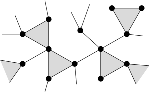
Figure 1: In the model proposed here, we separately specify the number of single edges and complete triangles (shaded) attached to each vertex.

The model we propose generalizes the standard “configuration model” of network theory, which is a model of a random graph with arbitrary degree distribution MR95 ; NSW01 . In that model one specifies the number of edges connected to each vertex. In our generalized model, pictured in Fig. 1, we specify both the number of edges and the number of triangles. For a network of $n$ vertices, we define $t_{i}$ to be the number of triangles in which vertex $i$ participates and $s_{i}$ to be the number of single edges other than those belonging to the triangles. That is, edges within triangles in this model are enumerated separately from edges that are placed singly note2 . We can think of a single edge as being a network element that joins together two vertices and a triangle as a different kind of element that joins three. In principle, one could generalize the model further to include higher-order elements of four or more vertices. The techniques described here can be extended in a straightforward fashion to such cases.

We can think of $s_{i}$ as specifying the number of ends or “stubs” of single edges that emerge from vertex $i$ and $t_{i}$ as specifying the number of corners of triangles. The complete joint degree sequence $\{s_{i},t_{i}\}$ specifies the numbers of such stubs and corners for every vertex. In simple cases the values of $s_{i}$ and $t_{i}$ may be uncorrelated, but correlated choices are also possible that allow us to reproduce more complex behaviors seen in some networks, such as variation of local clustering with degree Ravasz02 .

Given the degree sequence, we create our network by choosing pairs of stubs uniformly at random and joining them to make complete edges, and also choosing trios of corners at random and joining them to form complete triangles. The end result is a network drawn uniformly at random from the set of all possible matchings of stubs and corners. The only constraint is that, in order that there be no stubs or corners left over at the end of the process, the total number of stubs must be a multiple of 2 and the total number of corners a multiple of 3.

We define the joint degree distribution $p_{st}$ of our network to be the fraction of vertices connected to $s$ single edges and $t$ triangles—a quantity that can be easily measured for any observed network. Given this joint distribution, the conventional degree distribution of the network, the probability $p_{k}$ that a vertex has $k$ edges in total, both singly and in triangles, is

$$p_{k}=\sum_{s,t=0}^{\infty}p_{st}\delta_{k,s+2t},$$ (1)

since each triangle connected to a vertex contributes 2 to the degree and each single edge contributes 1. (Here $\delta_{ij}$ is the Kronecker delta.)

As with other random graph models, calculations for the model presented in this paper make use of probability generating functions. The generating function for the joint degree distribution of our network is a function of two variables thus:

$$g_{p}(x,y)=\sum_{s,t=0}^{\infty}p_{st}\,x^{s}y^{t}.$$ (2)

We can also write down a generating function for the total degree distribution $p_{k}$ thus:

$$f(z) =\sum_{k=0}^{\infty}p_{k}z^{k}=\sum_{k=0}^{\infty}\sum_{s,t=0}^{\infty}p_{st}\delta_{k,s+2t}z^{k}=\sum_{s,t=0}^{\infty}p_{st}z^{s+2t}$$

$$=g_{p}(z,z^{2}).$$ (3)

We can use these generating functions to calculate, for instance, the clustering coefficient $C$ of the network. The clustering coefficient can be defined as NSW01

$$C={3\times\mbox{(number of triangles in network)}\over\mbox{(number of connected triples)}}={3N_{\triangle}\over N_{3}},$$ (4)

where a connected triple means a single vertex connected by edges to two others. For the present model we have

$$3N_{\triangle} =n\sum_{st}tp_{st}=n\biggl{(}{\partial g_{p}\over\partial y}\biggr{)}_{x=y=1},$$ (5)

$$N_{3} =n\sum_{k}{k\choose 2}p_{k}=\mbox{$\frac{1}{2}$}n\biggl{(}{\partial^{2}f\over\partial z^{2}}\biggr{)}_{z=1},$$ (6)

and substituting into (4) then gives us the value of the clustering coefficient. Note that the factors of $n$ cancel out in the substitution, giving a value of $C$ that remains nonzero in the limit $n\to\infty$ so that the network always has clustering, by contrast with the configuration model and similar random graphs for which $C\to 0$.

A further quantity that will be important in the following calculations is the so-called excess degree distribution NSW01 . In the current model there are actually two different excess degree distributions:

$$q_{st}={(s+1)p_{s+1,t}\over\langle s\rangle},\qquad r_{st}={(t+1)p_{s,t+1}\over\langle t\rangle},$$ (7)

where $\langle s\rangle$ and $\langle t\rangle$ are the averages of $s$ and $t$ over all vertices. Here $q_{st}$ is the distribution of the number of edges and triangles attached to a vertex reached by traversing an edge, excluding the traversed edge, and $r_{st}$ is the corresponding distribution for a vertex reached by traversing a triangle. The generating functions for these distributions are

$$g_{q}(x,y) =\sum_{st}q_{st}x^{s}y^{t}={1\over\langle s\rangle}\sum_{st}sp_{st}x^{s-1}y^{t}={1\over\langle s\rangle}{\partial g_{p}\over\partial x},$$ (8)

$$g_{r}(x,y) =\sum_{st}r_{st}x^{s}y^{t}={1\over\langle t\rangle}\sum_{st}tp_{st}x^{s}y^{t-1}={1\over\langle t\rangle}{\partial g_{p}\over\partial y}.$$ (9)

One of the definitive features of any network is its giant component—the portion of the network that is connected into a single extensive group such that any vertex in the group can be reached from any other via the network. In a communication network, for example, the giant component corresponds to the fraction of vertices that can actually intercommunicate, the rest being isolated in disconnected small components. We can use our generating functions to calculate the size of the giant component in the clustered network.

Let $u$ be the mean probability that a vertex reached by traversing a single edge is not a member of the giant component and $v$ be the corresponding probability for a vertex reached by traversing a triangle. (Equivalently, $v^{2}$ is the probability that a triangle doesn’t lead to the giant component via either of the vertices at its other corners.) In order for a vertex at the end of a single edge not to belong to the giant component, all the other vertices to which it is connected, either by edges or by triangles, must also not be members of the giant component. If it is connected to $s$ other edges and $t$ triangles, then this happens with probability $u^{s}v^{2t}$. The generalized degrees $s$ and $t$ are distributed according to the excess degree distribution $q_{st}$ and, averaging over this distribution, we find

$$u=\sum_{st}q_{st}u^{s}v^{2t}=g_{q}(u,v^{2}).$$ (10)

By a similar argument we also find that

$$v=g_{r}(u,v^{2}).$$ (11)

Then the probability that a randomly chosen vertex is not in the giant component is $\sum_{st}p_{st}u^{s}v^{2t}=g_{p}(u,v^{2})$ and the expected size $S$ of the giant component as a fraction of the entire network is one minus this quantity:

$$S=1-g_{p}(u,v^{2}).$$ (12)

Between them, Eqs. (10)–(12) allow us to calculate the size of the giant component if there is one.

As an example, consider a network that has the doubly Poisson degree distribution

$$p_{st}=\mathrm{e}^{-\mu}{\mu^{s}\over s!}\,\mathrm{e}^{-\nu}{\nu^{t}\over t!},$$ (13)

where the parameters $\mu$ and $\nu$ are the average numbers of single edges and triangles per vertex respectively. Then

$$g_{p}(x,y)=g_{q}(x,y)=g_{r}(x,y)=\mathrm{e}^{\mu(x-1)}\mathrm{e}^{\nu(y-1)},$$ (14)

and $u=v=1-S$, leading to

$$S=1-\mathrm{e}^{-[\mu S+\nu S(2-S)]}.$$ (15)

This is a transcendental equation that has no closed-form solution (other than the trivial solution $S=0$) but it can easily be solved by numerical iteration starting from a suitable initial value. The right-hand panel of Fig. 2 shows the resulting giant component size as a function of clustering coefficient for a network with fixed average degree. As the figure shows, the size of the giant component falls off with increasing clustering coefficient, which happens because the triangles that give the network its clustering contain redundant edges that serve no purpose in connecting the giant component together. One edge out of every three in a triangle is redundant in this way. Thus for a given average degree, and hence a given total number of edges, fewer vertices can be connected together in a network of triangles than in a network of single edges.

Figure 2: Right panel: the size of the giant component in networks with the degree distribution of Eq. (13) and average degree $\mu+2\nu=2$, as a function of clustering coefficient. Left panel: the size of the giant cluster for percolation on the same networks for values of the clustering coefficient $C=0$, 0.1, 0.2, and 0.3, as a function of bond occupation probability $\phi$. Note that when $\phi=1$ the giant cluster and giant component have the same size, as indicated by the dotted lines.

We can also calculate the sizes of the small components in the network. Let $h_{q}(z)$ be the generating function for the distribution of number of vertices accessible, either directly or indirectly, via the vertex at the end of a single edge, and similarly for $h_{r}(z)$ and triangles. Then, by an argument analogous to that of NSW01 , we can show that

$$h_{q}(z)=zg_{q}(h_{q}(z),h_{r}^{2}(z)),\quad h_{r}(z)=zg_{r}(h_{q}(z),h_{r}^{2}(z)),$$ (16)

and the probability that a randomly chosen vertex anywhere in the network belongs to a component of a given size is generated by

$$h_{p}(z)=zg_{p}(h_{q}(z),h_{r}^{2}(z)).$$ (17)

Then, for example, the mean size of the component to which a vertex belongs is

$$h_{p}^{\prime}(1)=1+g_{p}^{(1,0)}(1,1)h_{q}^{\prime}(1)+2g_{p}^{(0,1)}(1,1)h_{r}^{\prime}(1),$$ (18)

where $g_{p}^{(m,n)}$ is $g_{p}$ differentiated $m$ times with respect to its first argument and $n$ times with respect to its second.

The derivatives $h_{q}^{\prime}(1)$ and $h_{r}^{\prime}(1)$ in Eq. (18) can be found from Eq. (16) by differentiating, setting $x=y=1$, and making use Eqs. (8) and (9), which gives

$$h_{q}^{\prime}(1) =1+{1\over\langle s\rangle}H_{xx}h_{q}^{\prime}(1)+{2\over\langle s\rangle}H_{xy}h_{r}^{\prime}(1),$$ (19)

$$h_{r}^{\prime}(1) =1+{1\over\langle t\rangle}H_{yx}h_{q}^{\prime}(1)+{2\over\langle t\rangle}H_{yy}h_{r}^{\prime}(1),$$ (20)

where the $H$ variables are the elements of the Hessian matrix $\mathbf{H}$ of second derivatives of $g_{p}$, evaluated at the point $x=y=1$:

$$H_{xx}=g_{p}^{(2,0)}(1,1),\qquad H_{xy}=g_{p}^{(1,1)}(1,1),$$ (21)

and so forth.

We can write Eqs. (19) and (20) in matrix form as $\mathbf{h}=\mathbf{1}+\boldsymbol{\alpha}^{-1}\mathbf{H}\boldsymbol{\beta}\cdot\mathbf{h}$, where the vectors $\mathbf{h}$ and $\mathbf{1}$ are $\mathbf{h}=(h_{q}^{\prime}(1),h_{r}^{\prime}(1))$ and $\mathbf{1}=(1,1)$ and the diagonal matrices $\boldsymbol{\alpha}$ and $\boldsymbol{\beta}$ are

$$\boldsymbol{\alpha}=\begin{pmatrix}\langle s\rangle&0\\ 0&\langle t\rangle\end{pmatrix},\qquad\boldsymbol{\beta}=\begin{pmatrix}1&0\\ 0&2\end{pmatrix}.$$ (22)

Rearranging yields $(\mathbf{I}-\boldsymbol{\alpha}^{-1}\mathbf{H}\boldsymbol{\beta})\cdot\mathbf{h}=\mathbf{1}$, where $\mathbf{I}$ is the identity matrix, and by inverting this equation and combining the result with Eq. (18) we can find the average component size.

The average will diverge at the point where $\det(\mathbf{I}-\boldsymbol{\alpha}^{-1}\mathbf{H}\boldsymbol{\beta})=0$ and, performing the derivatives in Eq. (21), we find the following condition for the point at which the giant component forms:

$$\biggl{[}{\langle s^{2}\rangle\over\langle s\rangle}-2\biggr{]}\biggl{[}2{\langle t^{2}\rangle\over\langle t\rangle}-3\biggr{]}=2{\langle st\rangle^{2}\over\langle s\rangle\langle t\rangle}.$$ (23)

In the case where there are no triangles in the network, this equation reduces to the well known criterion $\langle s^{2}\rangle/\langle s\rangle-2=0$ of Molloy and Reed MR95 for the phase transition in the ordinary configuration model. When triangles are present, Eq. (23) gives the appropriate generalization of that criterion.

We can calculate many other properties of our networks, including average path lengths and vertex connection probabilities. As our final example in this paper we demonstrate the calculation of percolation properties of random graphs with clustering. Both site and bond percolation processes on networks have important applications: site percolation is related to network resilience CEBH00 ; CNSW00 , while bond percolation is related to the dynamics of disease and other spreading processes Mollison77 ; Grassberger82 . Consider, for instance, a bond percolation process on our model network, with each edge in the network occupied independently with probability $\phi$. By analogy with our earlier calculations, let $u$ be the probability that a vertex is not connected to the percolating (giant) cluster of this percolation process via one of its single edges, and let $v^{2}$ be the corresponding probability for a triangle.

If a vertex is not connected to the giant cluster via a given single edge then one of two things must be true: either the edge is not occupied, which happens with probability $1-\phi$, or it is occupied but the vertex at its end is itself not connected to the giant cluster via any of its other edges or triangles of which, let us say, there are $s$ and $t$ respectively. This second process happens with probability $\phi u^{s}v^{2t}$. But $s$ and $t$ are by definition distributed according to the excess degree distribution $q_{st}$ and, averaging over this distribution, we then find that

$$u=1-\phi+\phi\sum_{st}q_{st}u^{s}v^{2t}=1-\phi[1-g_{q}(u,v^{2})].$$ (24)

The corresponding equation for triangles is more involved, but still essentially straightforward to derive:

$$v^{2}=1-2\phi(1-\phi^{2})[1-g_{r}(u,v^{2})]-\phi^{2}(3-2\phi)[1-g_{r}^{2}(u,v^{2})].$$ (25)

(Notice that Eqs. (24) and (25) reduce to Eqs. (10) and (11) for the giant component of the network, as they should, when $\phi=1$.)

Now the size $S$ of the giant cluster of the percolation process is given by $S=1-g_{p}(u,v^{2})$. The left-hand panel of Fig. 2 shows $S$ as a function of $\phi$ for the Poisson network of Eq. (13), for fixed average degree and several different values of the clustering coefficient. As the figure shows, higher clustering pushes the percolation transition toward lower values of $\phi$, which can be understood as an effect of the redundant paths introduced by the triangles in the network, which provide more opportunities to connect clusters together. At the same time, the ultimate size of the giant cluster as $\phi$ approaches 1 is smaller in more clustered networks and indeed becomes equal to the size of the giant component when $\phi=1$, as indicated by the dashed lines in the figure. Other properties of the percolation process can be calculated in a similar fashion, including the position of the percolation threshold, the mean size of small clusters, and the complete distribution of sizes of small clusters.

To conclude, we have proposed a random-graph model of a clustered network that is exactly solvable for many of its properties including component sizes, existence and size of a giant component, and percolation properties. The model answers a long-standing question in the study of networks by showing how to construct an unbiased ensemble of networks with clustering, and could form the basis for future investigations of the effects of clustering on many processes of interest, including epidemic processes, network resilience, and dynamical systems on networks.

The author thanks Brian Karrer and Lenka Zdeborova for useful conversations. This work was funded in part by the National Science Foundation under grant DMS–0804778.

References

- (1) A. Rapoport, Cycle distribution in random nets. Bulletin of Mathematical Biophysics 10, 145–157 (1968).
- (2) D. J. Watts and S. H. Strogatz, Collective dynamics of ‘small-world’ networks. Nature 393, 440–442 (1998).
- (3) M. A. Serrano and M. Boguñá, Clustering in complex networks: I. General formalism. Phys. Rev. E 74, 056114 (2006).
- (4) M. E. J. Newman and J. Park, Why social networks are different from other types of networks. Phys. Rev. E 68, 036122 (2003).
- (5) A.-L. Barabási and R. Albert, Emergence of scaling in random networks. Science 286, 509–512 (1999).
- (6) M. E. J. Newman, S. H. Strogatz, and D. J. Watts, Random graphs with arbitrary degree distributions and their applications. Phys. Rev. E 64, 026118 (2001).
- (7) R. Pastor-Satorras, A. Vázquez, and A. Vespignani, Dynamical and correlation properties of the Internet. Phys. Rev. Lett. 87, 258701 (2001).
- (8) M. E. J. Newman, Assortative mixing in networks. Phys. Rev. Lett. 89, 208701 (2002).
- (9) E. M. Jin, M. Girvan, and M. E. J. Newman, The structure of growing social networks. Phys. Rev. E 64, 046132 (2001).
- (10) P. Holme and B. J. Kim, Growing scale-free networks with tunable clustering. Phys. Rev. E 65, 026107 (2002).
- (11) K. Klemm and V. M. Eguiluz, Highly clustered scale-free networks. Phys. Rev. E 65, 036123 (2002).
- (12) M. A. Serrano and M. Boguñá, Tuning clustering in random networks with arbitrary degree distributions. Phys. Rev. E 72, 036133 (2005).
- (13) S. Bansal, S. Khandelwal, and L. A. Meyers, Evolving clustered random networks. Preprint arxiv:0808.0509 (2008).
- (14) A recent preprint of B. Bollobás, S. Janson, and O. Riordan [arxiv:0807.2040 (2008)] describes an interesting and general model capable of creating clustered networks among many other possibilities. Because of its complexity the model appears challenging to treat analytically and only a few results are known, but it is possible that for special cases calculations similar to those described in this paper could be carried out.
- (15) M. Molloy and B. Reed, A critical point for random graphs with a given degree sequence. Random Structures and Algorithms 6, 161–179 (1995).
- (16) It is possible for single edges by chance to form triangles themselves, but it is straightforward to show that, so long as mean degree remains constant as increases, the density of such triangles vanishes in the limit of large system size. Similarly the density of multiedges—of two vertices being connected by two or more different edges or triangles or a combination of the two—vanishes in the limit of large .
- (17) E. Ravasz, A. L. Somera, D. A. Mongru, Z. Oltvai, and A.-L. Barabási, Hierarchical organization of modularity in metabolic networks. Science 297, 1551–1555 (2002).
- (18) R. Cohen, K. Erez, D. ben-Avraham, and S. Havlin, Resilience of the Internet to random breakdowns. Phys. Rev. Lett. 85, 4626–4628 (2000).
- (19) D. S. Callaway, M. E. J. Newman, S. H. Strogatz, and D. J. Watts, Network robustness and fragility: Percolation on random graphs. Phys. Rev. Lett. 85, 5468–5471 (2000).
- (20) D. Mollison, Spatial contact models for ecological and epidemic spread. Journal of the Royal Statistical Society B 39, 283–326 (1977).
- (21) P. Grassberger, On the critical behavior of the general epidemic process and dynamical percolation. Math. Biosci. 63, 157–172 (1982).