Chaotic thermalization in Yang-Mills-Higgs theory on a spacial lattice

Abstract

We analyze the Hamiltonian time evolution of classical SU$\left(2\right)$ Yang-Mills-Higgs theory with a fundamental Higgs doublet on a spacial lattice. In particular, we study energy transfer and equilibration processes among the gauge and Higgs sectors, calculate the maximal Lyapunov exponents under randomized initial conditions in the weak-coupling regime, where one expects them to be related to the high-temperature plasmon damping rate, and investigate their energy and coupling dependence. We further examine finite-time and finite-size errors, study the impact of the Higgs fields on the instability of constant non-Abelian magnetic fields, and comment on the implications of our results for the thermalization properties of hot gauge fields in the presence of matter.

I Introduction

A variety of essential physical processes, ranging from ultrarelativistic heavy-ion collisions hei04 to the reheating period and phase transitions in the early Universe bas06 , proceed at least initially far from thermodynamic equilibrium and involve abundantly many nonperturbative degrees of freedom. The first-principle based theoretical treatment of such phenomena, which require a quantum field theoretic description but are inaccessible to Euclidean lattice simulations, is as a rule beyond present capabilities. Important exceptions to this rule arise, however, if the underlying amplitudes receive dominant contributions from classical fields. The latter may be provided, in particular, by bosonic long-wavelength modes at high temperature $T$ and with energies $E\ll T$ since the Bose-Einstein distribution supplies them with the large occupation numbers needed to ensure (semi-) classical behavior. In non-Abelian gauge theories, observables governed by such classical modes are typically of $O\left(g^{2}T\right)$ in the weak-coupling regime (where $g$ is the gauge coupling and $g^{2}T$ sets an inverse classical length scale) and have a finite classical limit. Prominent examples include the transport coefficients which control magnetic screening lin80 and color diffusion sel93 , and in particular the static plasmon damping rate bra90 . The latter has direct impact on the local energy and momentum equilibration processes among hot gauge-field quanta, which were found to occur over surprisingly short times of less than 1 fm/$c$ in the excited matter created by ultrarelativistic nuclear collisions at RHIC hei04 ; pis08 .

Essentially classical nonequilibrium observables of the above type may therefore be calculated by relating them to real-time evolution properties of classical long-wavelength gauge fields and by simulating those nonperturbatively on a spacial lattice mul92 ; bir294 . Along these lines, the plasmon damping rate was argued to be proportional to the classical gluon damping rate and, at least at weak coupling, further to the maximal Lyapunov exponent (MLE) which governs the exponential separation rate between initially neighboring random gauge-field configurations mul92 ; bir95 . The underlying reasoning is based on the expected ergodicity of the classical field trajectories and on the relation between exponential growth and damping rates provided by time reversal symmetry bir95 . In the weak-coupling region, furthermore, these relations can be tested quantitatively by comparison with results from partially resummed thermal perturbation theory or alternatively from kinetic theory bra90 ; bla02 .

Following up on the above arguments, the present paper will deal with the real-time evolution of classical SU$\left(2\right)$ Yang-Mills-Higgs (YMH) theory on spacial lattices of various sizes. A particular focus will be on the role of the scalar and hence classically treatable matter fields, provided by the fundamental Higgs doublet, in the chaotic dynamics. The center piece of the analysis is a systematic survey of the energy and coupling dependence of a set of maximal Lyapunov exponents designed to cover representative parts of the weakly coupled YMH phase space. Since our theory corresponds to the electroweak sector of the standard model with vanishing Weinberg angle, the resulting MLEs contain information which may be useful for understanding cosmological nonequilibrium processes during semiclassical evolution phases of the early Universe, including topological structure formation, baryogenesis pro97 and potentially cosmic string evolution hin95 .

Moreover, our results will be relevant for the analysis of local equilibration processes in the highly excited matter produced at the RHIC hei04 ; pis08 and soon the CERN LHC arm08 colliders. Indeed, the chaoticity of the gauge dynamics provides a natural mechanism for entropy production by soft fields (and the accompanying particle production in the quantum case), and its most unstable field modes contribute dominantly to equilibration processes. In particular, our results will give rise to new estimates for the energy and coupling dependence of the gauge-field damping rate in the presence of scalar matter. Furthermore, the MLEs should receive contributions from the non-Abelian plasma instabilities which were recently argued to accelerate the isotropization and thermalization processes in the aftermath of high-energy nuclear collisions mro06 . The underlying unstable modes could in principle be isolated by numerical techniques similar to ours. As in chaotic inflation scenarios, furthermore, such instabilities typically generate nonperturbatively large occupation numbers, which may extend the reliability of our classical treatment to larger couplings and lower temperatures. Some of our qualitative results may even be robust enough to provide guidance on the impact of fundamental quark fields.

Although our main focus will be on the evolution of random fields, we also study the impact of the Higgs fields on the instability of a constant non-Abelian magnetic field. The employed techniques may later be applied to more complex coherent fields, including classical solutions of YMH theory amb91 and gauge-invariant coherent soft modes for07 . Studies of this type could provide new insights into the corresponding quantum theories. Applied to multimonopole configurations of YMH theory with an adjoint Higgs field, whose chaotic interactions we have recently studied far05 , they may for example help to clarify the role of chaotic monopole ensembles in disordering the gauge-theory vacuum.

The paper is organized as follows: in Sec. II we summarize the formulation of SU$\left(2\right)$ YMH theory on a Hamiltonian lattice, derive the corresponding field equations and discuss suitable distance measures on the space of gauge and Higgs field configurations. Section III outlines the main ingredients of our numerical analysis, examines finite-time and finite-size effects, discusses the time evolution of the energy transfer between the various field sectors, and evaluates the rate of divergence between initially neighboring random field configurations at intermediate times. On this basis, we generate in Sec. IV a representative set of maximal Lyapunov exponents, discuss their energy dependence and relation to the plasmon damping rate, then extend the analysis by calculating a set of long-time Lyapunov histories, and finally evaluate the impact of the Higgs fields on the Savvidy instability of constant non-Abelian magnetic fields. Sec. V puts our results into context by discussing related nonequlibrium processes in the early Universe and in the aftermath of high-energy nuclear collisions, and Sec. VI summarizes our main findings and provides some conclusions.

II Yang-Mills-Higgs dynamics on a spacial lattice

In order to identify and measure chaotic properties of a dynamical system, one has to follow the evolution of its dynamical variables over sufficiently long periods of time. A numerical treatment of field theories further requires to approximate space by a discrete lattice. The analogous handling of the time variable (as typically implemented in Euclidean spacetime subject to periodic boundary conditions) is unsuitable for chaos investigations, however, since it would unacceptably restrict the accessible evolution times. Hence we resort to the Hamiltonian formulation of lattice field theory kog75 in Minkowski space where gauge fields are restricted to temporal gauge and time remains an unbounded and (in principle) continuous variable. A further benefit of this formulation is that residual gauge symmetries enforced by Gauss’ law can be accurately preserved during time evolution. In the following subsections we briefly summarize this approach as it applies to YMH theory and define the distance measures needed to determine the Lyapunov exponents. (More details can be found e.g. in Refs. kog75 ; chi85 .)

II.1 Hamiltonian lattice setup

In the following section we outline pertinent aspects of the Hamiltonian formulation of 3+1 dimensional SU$\left(2\right)$ Yang-Mills-Higgs theory on a spacial cubic lattice subject to periodic boundary conditions. Since the Higgs field $\phi$ is taken to transform in the fundamental representation of the gauge group, this theory is equivalent to the electroweak sector of the standard model in the limit of vanishing Weinberg angle. The gauge is fixed to $A_{0}^{a}=0$, i.e. to Weyl gauge. The unbroken phase corresponding to a gauge-matter plasma is selected by positive Higgs mass and interaction terms, which allows for comparison of the results with (hard-thermal-loop resummed) perturbative results at high temperature below.

The corresponding YMH Hamiltonian can thus be written as

$$H=a^{3}\sum_{x,i}\tfrac{1}{2}E_{x,i}^{a}E_{x,i}^{a}+\frac{4}{g^{2}a}\sum_{x}\sum_{1\leq i<j\leq 3}\!\left(1-\tfrac{1}{2}trU_{x,ij}\right)$$ (1)

$$+\,a^{3}\sum_{x}\tfrac{1}{2}tr\left(\dot{\phi}{}_{x}^{\dagger}\dot{\phi}{}_{x}\right)-a\sum_{x,i}tr\left(\phi_{x}^{\dagger}U_{x,i}\phi_{x+i}\right)$$

$$+a\sum_{x}\tfrac{1}{2}tr\left(\phi_{x}^{\dagger}\phi_{x}\right)\left[6+a^{2}\kappa\tfrac{1}{2}tr\left(\phi_{x}^{\dagger}\phi_{x}\right)\right]$$

where $g$ is the gauge coupling, $\kappa$ the Higgs self-coupling, $a$ the lattice spacing and dots denote time derivatives. The non-Abelian magnetic field is described by the spacial plaquette

$$U_{x,ij}\equiv U_{x,i\,}U_{x+i,j\,}U_{x+j,i\,}^{-1}U_{x,j}^{-1}\overset{a\rightarrow 0}{\longrightarrow}\exp\left(-iga^{2}F_{x,ij}+O\left(a^{3}\right)\right)$$ (2)

(with $i,j\in\left\{1,2,3\right\}$ and $i\neq j$), i.e. by the ordered minimal-circumference loop constructed from the link variables

$$U_{x,i}=\exp\left(-igaA_{x,i}\right)$$ (3)

where $A_{x,i}=A_{x,i}^{a}t^{a}$ is the gauge field and $\sigma^{a}=2t^{a}$ with $a\in\left\{1,2,3\right\}$ are the Pauli matrices. The $U_{x,i}$ are defined on the link which connects the site $x$ with its neighbor in the positive $i$ direction. Hence the spacial plaquettes contain the non-Abelian magnetic field strength components $F_{x,ij}=\frac{1}{a}\left(A_{x+i,j}-A_{x,j}-A_{x+j,i}+A_{x,i}\right)-ig\left[A_{x,i},A_{x,j}\right]$ while their electric counterparts $E_{x,i}^{a}=-\dot{A}_{x,i}^{a}$ are independent variables. The first term of the Hamiltonian (1) therefore describes the energy residing in the electric fields while the second term,

$$H_{\text{mag}}=\frac{4}{g^{2}a}\sum_{x}\sum_{1\leq i<j\leq 3}\!\left(1-\tfrac{1}{2}trU_{x,ij}\right)\overset{a\rightarrow 0}{\longrightarrow}a^{3}\sum_{x,i,j}\tfrac{1}{4}F_{x,ij}^{a}F_{x,ij}^{a}+O\left(a^{4}\right),$$ (4)

approaches the magnetic or potential energy of the gauge field in the naive continuum limit.

For the numerical implementation of the SU$\left(2\right)$ link variables we have adopted the quaternion representation

$$U=u^{0}-i\vec{u}\cdot\vec{\sigma}=\left(\begin{tabular}[]{ll}$u^{0}-iu^{3},$&$-u^{2}-iu^{1}$\\ $u^{2}-iu^{1},$&$u^{0}+iu^{3}$\end{tabular}\right)$$ (5)

(the indices $x,i$ are suppressed) whose real components $u^{\mu}=\left(u^{0},\vec{u}\right)\in R,$ $\mu\in\left\{0,1,2,3\right\}$ satisfy the constraint $\det U=u^{0}u^{0}+u^{a}u^{a}=1$ and thereby ensure unitarity $UU^{\dagger}=1$ as well. The $u^{\mu}$ are thus (four dimensional, cartesian) coordinates on the SU$\left(2\right)$ group manifold $S^{3}$. The representation (5) leads to simple field equations (cf. Sec. II.2) and requires the minimal number of floating point operations to calculate the product $UV=u^{0}v^{0}-u^{a}v^{a}-i\sigma^{a}\left(u^{0}v^{a}+v^{0}u^{a}+\varepsilon^{abc}u^{b}v^{c}\right)$ of two link variables. In order to state the initial conditions for the time evolution of the gauge field, however, we prefer the alternative representation of the link variable as a rotation of angle $\omega_{\text{G}}$ around the direction $\hat{n}\left(\vartheta,\varphi\right)$, i.e.

$$U=\exp\left(-igA^{a}\frac{\sigma^{a}}{2}\right)=\cos\left(\frac{\omega_{\text{G}}}{2}\right)-i\hat{n}\cdot\vec{\sigma}\sin\left(\frac{\omega_{\text{G}}}{2}\right)$$ (6)

(suppressing again the indices). In terms of the polar angles $0\leq\omega_{\text{G}}\leq 2\pi$, $0\leq\vartheta_{\text{G}}\leq\pi$ and $0\leq\varphi_{\text{G}}\leq 2\pi$ one then has $gA^{a}=\omega_{\text{G}}\hat{n}^{a}$ with $\hat{n}^{a}=\left(\sin\vartheta_{\text{G}}\cos\varphi_{\text{G}},\sin\vartheta_{\text{G}}\sin\varphi_{\text{G}},\cos\vartheta_{\text{G}}\right)$ and $u^{0}=\cos\left(\omega_{\text{G}}/2\right)$, $u^{a}=\hat{n}^{a}\sin\left(\omega_{\text{G}}/2\right)$. The Higgs field $\phi_{x}$ in the fundamental representation of the gauge group is written in an analogous quaternion representation,

$$\phi=\phi^{0}-i\vec{\phi}\cdot\vec{\sigma}=R\left[\cos\left(\frac{\omega_{\text{H}}}{2}\right)-i\hat{n}\cdot\vec{\sigma}\sin\left(\frac{\omega_{\text{H}}}{2}\right)\right],$$ (7)

where the polar decomposition again turns out to be more suitable for stating the initial conditions (cf. Sec. III.1). In contrast to the unitary link variables $U$, however, the (square) modulus

$$R^{2}=\frac{1}{2}tr\left(\phi^{\dagger}\phi\right)$$ (8)

of the Higgs field remains unconstrained.

Exploiting its (classical) scaling properties, the YMH Hamiltonian (1) can be reexpressed in terms of the dimensionless variables $\bar{H}=g^{2}aH$, $\bar{E}{}_{x,i}^{a}=ga^{2}E_{x,i}^{a}$, $\bar{\phi}{}_{x}=ga\phi_{x}$, $\bar{\kappa}=\kappa/g^{2}$ and $\bar{t}=t/a$ as

$$\bar{H}=\sum_{x}\left[\varepsilon_{\text{G,el}}\left(x\right)+\varepsilon_{\text{G,mag}}\left(x\right)+\varepsilon_{\text{H,kin}}\left(x\right)+\varepsilon_{\text{H,pot}}\left(x\right)+\varepsilon_{\text{G-H}}\left(x\right)\right]$$ (9)

with the dimensionless energy densities

$$\varepsilon_{\text{G,el}}\left(x\right) = \sum_{i}\tfrac{1}{2}\bar{E}{}_{x,i}^{a}\bar{E}{}_{x,i}^{a},\text{ \ \ \ \ }\varepsilon_{\text{G,mag}}\left(x\right)=4\sum_{1\leq i<j\leq 3}\!\left(1-\frac{1}{2}trU_{x,ij}\right),$$ (10)

$$\varepsilon_{\text{H,kin}}\left(x\right) = \frac{1}{2}tr\left(\dot{\bar{\phi}}{}_{x}^{\dagger}\dot{\bar{\phi}}{}_{x}\right),\text{ \ \ \ \ \ \ }\varepsilon_{\text{G-H}}\left(x\right)=-\sum_{i}tr\left(\bar{\phi}{}_{x}^{\dagger}U_{x,i}\bar{\phi}{}_{x+i}\right),$$ (11)

$$\varepsilon_{\text{H,pot}}\left(x\right) = 3tr\left(\bar{\phi}{}_{x}^{\dagger}\bar{\phi}{}_{x}\right)+\frac{\bar{\kappa}}{4}\left[tr\left(\bar{\phi}{}_{x}^{\dagger}\bar{\phi}{}_{x}\right)\right]^{2},$$ (12)

where the fields are now functions of $\bar{t}$ and dots represent $d/d\bar{t}$. The above form of the Hamiltonian renders the dependence on the total energy $\bar{H}$ and the Higgs self-coupling $\bar{\kappa}$, i.e. the two physical parameters of the YMH system, explicit (whereas the lattice spacing $a$ and the gauge coupling $g$ are absorbed into the dimensionless variables and fields).

II.2 Field equations

The YMH Hamiltonian (9) generates the classical time evolution of electric, magnetic and Higgs fields. This becomes explicit in the corresponding first-order Hamilton equations which we derive with the help of the Poisson brackets

$$\left\{X,\bar{H}\right\}\equiv\frac{\partial X}{\partial q_{s}}\,\frac{\partial\bar{H}}{\partial p_{s}}-\frac{\partial X}{\partial p_{s}}\,\frac{\partial\bar{H}}{\partial q_{s}}$$ (13)

of the dynamical variables $X$ with the Hamiltonian $\bar{H}$ (where $q_{s},p_{s}$ are the canonically conjugate variables and summation over $s$ is implied). According to the canonical formalism, the time dependence of $X$ is then determined by its Hamilton equation

$$\dot{X}=\frac{1}{g^{2}}\left\{X,\bar{H}\right\}.$$ (14)

Specializing Eq. (14) to the link variable $U_{x,i}$ and abbreviating $l\equiv\left\{x,i\right\}$ leads with

$$\left\{\bar{E}{}_{l}^{a},U_{m}\right\}=-ig^{2}t^{a}U_{m}\delta_{lm}$$ (15)

to the equation of motion

$$\dot{U}{}_{l}=\frac{1}{g^{2}}\left\{U_{l},\bar{H}\right\}=i\bar{E}{}_{l}U_{l}\quad$$ (16)

where $\bar{E}{}_{l}=\bar{E}{}_{l}^{a}t^{a}$. In the quaternion representation (5) this equation reads

$$\dot{u}{}_{l}^{0}=\frac{1}{2}\bar{E}{}_{l}^{a}u_{l}^{a},~{}\ \ \ \ \ \dot{u}{}_{l}^{a}=-\frac{1}{2}\left(\bar{E}{}_{l}^{a}u_{l}^{0}+\epsilon^{abc}\bar{E}{}_{l}^{b}u_{l}^{c}\right)$$ (17)

and maintains, in particular, the time-independence of the unitarity constraint, i.e.

$$\dot{u}{}_{l}^{0}u_{l}^{0}+\dot{u}{}_{l}^{a}u_{l}^{a}=0.$$ (18)

Hamilton’s equation for the non-Abelian electric field strengths $\bar{E}{}_{x,i}^{a}$, which are the canonically conjugate momenta of the link variables, similarly becomes

$$\dot{\bar{E}}{}_{x,i}^{a}=\frac{1}{g^{2}}\left\{\bar{E}{}_{x,i}^{a},\bar{H}\right\}=\frac{i}{2}\sum_{j}tr\left[\sigma^{a}\left(U_{x,ij}-U_{x,ij}^{-1}\right)\right]+\frac{i}{2}tr\left(\bar{\phi}{}_{x}^{\dagger}\sigma^{a}U_{x,i}\bar{\phi}{}_{x+i}\right)$$ (19)

where the sum goes over the four plaquettes which contain the link $\left\{x,i\right\}$.

The Hamilton equations for the Higgs field, its canonical momentum $\pi$ and their Hermitian conjugates are analogously found to be

$$\dot{\bar{\phi}}_{x} = \frac{1}{g^{2}}\left\{\bar{\phi}_{x},\bar{H}\right\}=\frac{g}{a}\pi_{x}^{\dagger}=\tfrac{1}{2}tr\left(\dot{\bar{\phi}}_{x}\right)$$ (20)

$$\dot{\bar{\phi}}{}_{x}^{\dagger} = \frac{1}{g^{2}}\left\{\bar{\phi}_{x}^{\dagger},\bar{H}\right\}=\frac{g}{a}\pi_{x}$$ (21)

and

$$\dot{\pi}_{x} = \frac{1}{g^{2}}\left\{\pi_{x},\bar{H}\right\}=-\frac{a}{2g}tr\left\{\left[6+\bar{\kappa}tr\left(\bar{\phi}{}_{x}^{\dagger}\bar{\phi}{}_{x}\right)\right]\bar{\phi}{}_{x}^{\dagger}-2\sum_{i}\bar{\phi}{}_{x-i}^{\dagger}U_{x-i,i}\right\},$$ (22)

$$\dot{\pi}_{x}^{\dagger} = \frac{1}{g^{2}}\left\{\pi_{x}^{\dagger},\bar{H}\right\}=-\frac{a}{2g}tr\left\{\left[6+\bar{\kappa}tr\left(\bar{\phi}{}_{x}^{\dagger}\bar{\phi}{}_{x}\right)\right]\bar{\phi}{}_{x}-2\sum_{i}U_{x,i}\bar{\phi}{}_{x+i}\right\}.$$ (23)

In order to prepare for an efficient numerical solution of this system, we rewrite it in terms of two second-order equations,

$$\ddot{\bar{\phi}}{}_{x} = -\bar{\kappa}tr\left(\bar{\phi}{}_{x}^{\dagger}\bar{\phi}{}_{x}\right)\bar{\phi}{}_{x}-6\,\bar{\phi}{}_{x}+2\sum_{i}U_{x,i}\bar{\phi}{}_{x+i},$$ (24)

$$\ddot{\bar{\phi}}{}_{x}^{\dagger} = -\bar{\kappa}tr\left(\bar{\phi}{}_{x}^{\dagger}\bar{\phi}{}_{x}\right)\bar{\phi}{}_{x}^{\dagger}-6\,\bar{\phi}{}_{x}^{\dagger}+2\sum_{i}\bar{\phi}{}_{x-i}^{\dagger}U_{x-i,i},$$ (25)

and then combine those, by adding the Hermitian conjugate of Eq. (25) to Eq. (24), into

$$\ddot{\bar{\phi}}{}_{x}=-\bar{\kappa}tr\left(\bar{\phi}{}_{x}^{\dagger}\bar{\phi}{}_{x}\right)\bar{\phi}{}_{x}-6\,\bar{\phi}{}_{x}+\sum_{i}\left(\,U_{x,i}\bar{\phi}{}_{x+i}+U_{x-i,i}^{-1}\bar{\phi}{}_{x-i}\right).$$ (26)

Finally, we recall that the full YMH dynamics in temporal gauge is only recovered after supplementing Hamilton’s equations (17), (19) and (26) by Gauss’ law

$$\sum_{i=1}^{3}\left[\bar{E}_{x,i}^{a}-\frac{1}{2}tr\left(U_{x,-i}^{-1}\sigma^{a}U_{x,-i}\sigma^{b}\right)\bar{E}_{x-i,i}^{b}\right]=\bar{\rho}_{x}^{a}$$ (27)

which acts as a constraint. Since its Poisson bracket with the Hamiltonian (9) vanishes, Gauss’ law is preserved under time evolution. Above, we have defined the dimensionless non-Abelian charge density

$$\bar{\rho}_{x}^{a}=\frac{1}{2}tr\left[\text{Im}\left(\dot{\bar{\phi}}_{x}^{\dagger}\bar{\phi}_{x}\sigma^{4-a}\right)\right]$$ (28)

carried by the Higgs field.

II.3 Distance measures for gauge and Higgs field configurations

The chaotic behavior of dynamical systems reveals itself in an exponential sensitivity of their time evolution to small changes in the initial conditions. The quantitative characterization of this sensitivity requires a distance measure on the field configuration space (i.e. a metric). More specifically, in the YMH system one has to monitor the separation between a reference configuration $(U_{l},\phi)$ and its neighbor $(U_{l}^{\prime},\phi^{\prime})=(U_{l}+\delta U,\phi+\delta\phi)$. We will use individual distance measures in the gauge and Higgs sectors for this purpose, in order to determine the distance growth rate between two initially nearby gauge and Higgs field configurations individually.

In the gauge sector, we adopt the gauge-invariant metric mul92

$$d_{\text{G}}[U_{l},U_{l}^{\prime}]=\frac{1}{2N_{\text{p}}}\sum_{p}\,\left|trU_{p}-trU_{p}^{\prime}\right|$$ (29)

(where $N_{\text{p}}=3N^{3}$ is the total number of plaquettes on a lattice with $N$ sites per spacial dimension) to measure the distance between gauge-field configurations. In the continuum limit the distance measured by the metric (29) becomes proportional to the difference between the potential energies of reference and neighboring gauge fields. In the Higgs sector we employ the metric bir94

$$d_{\text{H}}[\phi,\phi^{\prime}]=\frac{1}{N^{3}}\sum_{x}\,\left|\left(R_{x}\right)^{2}-\left(R_{x}^{\prime}\right)^{2}\right|$$ (30)

which is gauge invariant as well.

Since the lattice gauge group, and consequently the $3\left(N_{c}^{2}-1\right)N^{3}$ dimensional space of magnetic SU$\left(N_{c}\right)$ gauge-field configurations on a lattice with $N$ sites per dimension, is compact and of nontrivial topology, more and more field configurations approach the same distance $d_{\text{G}}$ when $N$ increases. For the same reason, the distance (29) is bounded from above, and for fixed total energy an analogous bound applies to the whole phase space. These bounds lead to an eventual saturation of the distance growth. Although this does not limit the principal effectiveness of the measures $d_{\text{G,H}}$ for determining the Lyapunov exponents (see below), it adds to the typical “finite-time” uncertainties encountered in their numerical analysis. Other sources of finite-time errors arise from the need to extrapolate the numerical results to the $t\rightarrow\infty$ limit in which the MLEs are formally defined, and for $N\rightarrow\infty$ from the exponentially growing distances between chaotic trajectories which eventually overburden the floating point number representation capacities of any computer.

The standard approach for keeping finite-time errors of MLEs under control is to periodically rescale the distances ben80 after time intervals $\tau$ and to extrapolate the numerical results for $\ln d_{\text{G,H}}\left(t\right)/t$ to infinite times. This approach has been used to calculate several MLEs in non-Abelian gauge theories bir94 ; gon94 ; mue96 ; hei97 and to determine the whole Lyapunov spectrum on small lattices gon94 . We have adopted the same technique for the calculation of several long-time trajectories to be discussed in Secs. III.2 and IV.3. In these cases, we found it advantageous to employ the alternative distances measure

$$d_{\text{G}}^{\left(\text{alt}\right)}[U_{l},\bar{E}_{l};U_{l}^{\prime},\bar{E}_{l}^{\prime}]=\left\{\sum_{l}\left[\left(\bar{E}_{l}-\bar{E}_{l}^{\prime}\right)^{2}+\left(U_{l}-U_{l}^{\prime}\right)^{2}\right]\right\}^{1/2}$$ (31)

in the phase space of the gauge fields, which is a variant of the measure used in Ref. hei97 , and

$$d_{\text{H}}^{\left(\text{alt}\right)}[\bar{\phi},\bar{\phi}^{\prime}]=\left\{\sum_{x}\sum_{\alpha=0}^{3}\left[\left(\dot{\bar{\phi}}_{x}^{\alpha}-\dot{\bar{\phi}}_{x}^{\alpha\prime}\right)^{2}+\left(\bar{\phi}_{x}^{\alpha}-\bar{\phi}_{x}^{\alpha\prime}\right)^{2}\right]\right\}^{1/2},$$ (32)

adopted from Ref. hei97 , in the Higgs sector. Of course, the resulting Lyapunov exponents should not depend on the choice of distance measure. We have checked this for several examples and confirmed that the deviations between the MLE values obtained from the metrics (29), (30) and (31), (32) indeed remain well below the one-percent level.

Nevertheless, even under rescaling the practically achievable evolution times remain limited by the available computer resources. In fact, even in pure SU$\left(2\right)$ Yang-Mills theory mue96 systematic extrapolation errors turned out to become negligible only after evolution times of the order of $10^{5}$ lattice units. To make matters worse, we will find below that the equilibration between gauge and Higgs fields proceeds at a far slower pace than among the gauge fields alone (cf. Sec. III.2), and that as a consequence substantially longer evolution times are required to suppress such extrapolation errors in YMH theory. Adherence to one of our main goals, namely to calculate a rather exhaustive set of MLEs in the weak-coupling parameter and phase space, will therefore require a compromise. Indeed, to cover the relevant initial parameter space (on lattices of several different sizes) requires the calculation of $O\left(10^{2}\right)$ trajectory pairs and thus forces us to limit the individual evolution times.

Fortunately, size and systematics of finite-time errors can be estimated on the basis of the long-time energy balance (cf. Sec. III.2) and a few long-time orbits (cf. Sec. IV.3). Since we are mainly interested in the systematic energy-, coupling- and lattice-size dependence of the MLEs (rather than in their precise numerical values), furthermore, the competing goals of error suppression and calculability can be reconciled reasonably well. Our compromise will be to follow the majority of our distance histories only until they have saturated (without rescaling), which yields sufficiently accurate MLE estimates for most of our purposes. Rescaling will be used, on the other hand, for the long-time trajectories which we need to examine the energy transfer and equilibration processes between the gauge and Higgs field sectors in Sec. III.2, and for the analysis of the MLE’s finite-time errors and saturation properties in Sec. IV.3.

III Field initialization, energy balance and distance evolution

In the following section we discuss in turn the initialization of the neighboring field configurations, the distribution of the total energy over the different field sectors, and the time evolution of the distance between initially adjacent field configurations.

III.1 Initial conditions

Our first task will be to generate a representative set of phase-space trajectories for pairs of specifically initialized reference YMH fields $(U_{l},\phi)$ and their neighboring configurations $(U_{l}^{\prime},\phi^{\prime})=(U_{l}+\delta U,\phi+\delta\phi)$ at sufficiently small distances $d_{\text{G}}[U_{l},U_{l}^{\prime}]$ and $d_{\text{H}}[\phi,\phi^{\prime}]$. The resulting distance evolution histories will provide one of the foundations for our subsequent analysis of the maximal Lyapunov exponents. In the present subsection, we select a set of 77 initial conditions for the reference trajectories such that the weak-coupling region of the YMH phase space is covered with sufficient resolution. In order to allow for direct comparison with a previously calculated MLE, we follow the initialization procedure of Ref. hei97 . The resulting sample of field-pair trajectories will be considerably larger than that of preceding MLE calculations in gauge theories and include results from substantially larger lattice volumes (with up to 30³ sites).

In order to satisfy Gauss’ law (27) initially (and consequently over the whole time evolution), we set the non-Abelian electric field and the time derivative of the Higgs field at the initial time $\bar{t}_{0}=0$ equal to zero, i.e.

$$\bar{E}{}_{x,i}^{a}\left(0\right)=0,\text{ \ \ \ \ }\dot{\bar{\phi}}{}_{x}\left(0\right)=0,$$ (33)

which implies $\bar{\rho}_{x}^{a}\left(0\right)=0$ (cf. Eq. (28)). Hence the initial kinetic energies of all fields vanish while the potential energies are finite and ensure that the system starts far from equilibrium. The link variables $U_{l}$ are initialized by randomly choosing the isospin directions $\vartheta_{\text{G}},\varphi_{\text{G}}$ of the gauge potential $A_{l}^{a}=\omega_{\text{G,}l}\hat{n}{}_{l}^{a}(\vartheta_{\text{G},l},\varphi_{\text{G},l})$ from their full domains, while the initial value of the amplitude $\omega_{\text{G}}$ is chosen randomly over the restricted domain $\omega_{\text{G,}l}\in[0,2\pi\delta]$ with $\delta\leq 1$. The value of the parameter $\delta$ therefore controls the average gauge-field energy per plaquette, $\bar{E}_{\text{p}}\left(\delta\right)$, which grows as $\delta^{2}$ for $\delta\ll 1$ and saturates in the limit $\delta\rightarrow 1$ at the value $\bar{E}_{\text{p}}=4$ (cf. Fig. 1). The upper bound on $\bar{E}_{\text{p}}$ arises from the fact that the magnetic part (4) of the Hamiltonian (1) is uniformly bounded by the SU$\left(2\right)$ group volume, $\bar{H}_{\text{mag}}=ag^{2}H_{\text{mag}}\leq 24N^{3}$. The Higgs field (7), finally, is initialized by choosing its angular variables $\omega_{\text{H}}$, $\vartheta_{\text{H}}$ and $\varphi_{\text{H}}$ randomly from their full domains while keeping the dimensionless amplitude $\bar{R}_{x}\equiv gaR_{x}$ fixed at the same value $\bar{R}$ for all $\vec{x}$. As a consequence, the initial (potential) energy of the Higgs field is determined by the amplitude $\bar{R}$ and the coupling $\bar{\kappa}$.

The above initialization scheme characterizes any phase-space trajectory on a given lattice by three parameters $\delta$, $\bar{R}$ and $\bar{\kappa}$ which determine the average initial energy of both the gauge and Higgs fields. In addition, we will vary the lattice size, specified by the number $N$ of sites per dimension, so that each of our field-pair histories can be uniquely labeled by a quadruple of values for $\delta,\bar{R},\bar{\kappa}$ and $N$. Our maximal lattice size with $N=30$ is chosen to substantially reduce potential finite-size effects of previous studies bir94 ; hei97 ; bir96 on considerably smaller lattices. The main benefit of the random angle initialization is that it equips the initial configurations with a specific average energy density, or equivalently with a temperature $T$ which the fields will reach after equilibration. In our context, this is important because the temperature dependence of the MLEs is used to relate them to the static plasmon damping rates. Moreover, the resulting MLE values will turn out to be (within errors) independent of the random part of a given starting configuration, which indicates that the autocorrelation functions of the fields have decayed sufficiently strongly before the MLEs are measured (see below).

In order to stay safely inside the validity range of the semiclassical approximation, and to be able to relate our findings to perturbative results, we will restrict our simulations to the weak-coupling regime. As pointed out in Ref. hei97 , this requires that the energy contributed by the Higgs mass term dominates over the Higgs self-interaction energy, i.e.

$$\bar{\kappa}\bar{R}^{2}<1,$$ (34)

and that the magnetic gauge-field energy dominates over the gauge-Higgs interaction energy (which implies a weak gauge-Higgs coupling), or

$$\bar{R}^{2}<\delta$$ (35)

(for maximal field amplitudes). Both conditions also improve the eventual equipartition of the electric, magnetic and Higgs field energies because they prevent the total energy from strongly exceeding the bounded magnetic energy. The lower bound (35) on $\delta$ additionally limits finite-size effects [cf. Eq. (39)]. Furthermore, $\delta$ values too close to 1 should be avoided in order to keep lattice-spacing artefacts under control and to remain sufficiently close to the continuum limit (cf. Eq. (38)).

For each of the initial reference configurations $(U_{l},\phi)$ created according to the above procedure, we also generate a neighboring configuration $(U_{l}^{\prime},\phi^{\prime})$ separated from $(U_{l},\phi)$ by distances $d_{\text{G}}(t=0)\lesssim 5\times 10^{-7}\$and $d_{\text{H}}(t=0)\lesssim 10^{-17}$. This is achieved by randomly choosing slight variations of all the reference configuration’s field angles in the range $\delta\omega_{\text{G}}$, $\delta\vartheta_{\text{G}}$, $\delta\varphi_{\text{G}}$, $\delta\omega_{\text{H}}$, $\delta\vartheta_{\text{H}}$, $\delta\varphi_{\text{H}}\in\left[-\varepsilon,\varepsilon\right]$ where $\varepsilon=10^{-6}$. We then integrate the field equations of Sec. II.2 for each of these configuration pairs by means of a fourth-order Runge-Kutta algorithm and determine the time evolution of the distances $d_{\text{G}}$ and $d_{\text{H}}$. The integration time step should be much shorter than the lattice spacing $a$, and is additionally chosen small enough to ensure energy conservation with an accuracy of more than eight significant digits (after each step). The maximal violation of the constraints $\det{U}_{l}{=1}$ after a single time step of length $\Delta t=10^{-4}a$ is then about $10^{-12}$ at each link. In order to avoid the accumulation of these round-off errors, we further rescale the link variables after each step such that their determinant remains exactly unity (and Eq. (18) exactly satisfied). We convinced ourselves that Gauss’ law (27) then remains satisfied to better than five significant digits after each integration step.

III.2 Energy distribution over gauge and Higgs fields

We now turn to the energy transfer processes between the electric, magnetic and Higgs fields which contain crucial information on the nonequilibrium dynamics and quantitative thermalization properties of the YMH system. In our context, this information will be particularly helpful for understanding, qualitatively estimating and reducing the finite-time errors which afflict the calculation of the MLEs, and for putting the relation between the MLEs and the plasmon damping rates on a more solid footing. For several long-time trajectories, we have therefore recorded the evolution of the energies per degree of freedom stored in the electric field, $E_{\text{el}}=H_{\text{el}}/\left(6N^{3}\right)$, in the magnetic gauge field, $E_{\text{mag}}=H_{\text{mag}}/\left(6N^{3}\right)$, and in the Higgs field, $E_{\text{H}}=H_{\text{H}}/\left(4N^{3}\right),$ over the unprecedentedly long time periods $0\leq t\leq 20000a$ . In the following, we will often express the total energy (per degree of freedom) $E_{\text{G}}$ of the gauge field in terms of the average energy per plaquette $E_{\text{p}}$ as

$$E_{\text{G}}=E_{\text{el}}+E_{\text{mag}}=\frac{1}{2}E_{\text{p}},$$ (36)

and frequently encounter the total YMH energy per degree of freedom, $E=\left(6E_{\text{G}}+4E_{\text{H}}\right)/10$, as well.

Typical results for the time evolution of the different energies are plotted in Fig. 2 with $\delta=0.2$, $\bar{R}=0.2$, $\bar{\kappa}=$ $1$, $N=10$ and in Fig. 3 with $\delta=1$ and otherwise unchanged initial values. They confirm and extend the observation of Ref. hei97 that the energy equilibration between the electric, magnetic and Higgs field sectors of YMH theory proceed over two drastically different time scales (at least in the weak-coupling regime). Indeed, even when initialized in highly nonequilibrium configurations, as selected in Sec. III.1, the electric and magnetic gauge sectors can be seen to equilibrate very rapidly, namely after only a few lattice time units $a$. The Higgs field’s potential and kinetic energies, which are not shown separately in Figs. 2 and 3, equilibrate over an approximately equal relaxation time. (Generally the gauge and Higgs sectors reach different temperatures, however, according to the amount of energy stored in them by the initial conditions.) In contrast, the mutual thermalization of gauge and Higgs sectors typically requires 4 to 5 orders of magnitude more time. In fact, the energy transfer between the two sectors becomes appreciable only after a few hundred time units and takes several thousand more to essentially complete for $\delta=1$, and many more for $\delta=0.2$. Moreover, for the maximal $\delta=1$ moderate deviations from complete equipartition of the energy remain visible in Fig. 3 even after 10000 time units have elapsed. This may be a consequence of lattice-spacing artefacts which are maximal at $\delta=1$ (cf. Sec. III.1). The huge discrepancy between the two characteristic relaxation scales can be largely attributed to the initial conditions of Sec. III.1 which keep the system close to the weak-coupling and continuum limits.

The gauge-field energy (36) can be directly related to the temperature $T$ which the gauge fields reach after times $t\gg\lambda^{-1}$ (where $\lambda$ is the MLE). At sufficiently weak coupling (among the field oscillators) one has amb92

$$T=\frac{3}{2\left(N_{c}^{2}-1\right)}E_{\text{p}}$$ (37)

for the gauge group SU$\left(N_{c}\right)$ and thus $E_{\text{G}}=T$ for $N_{c}=2$. This relation will be relevant for the evaluation and interpretation of the MLEs which we extract in Sec. IV.1 from the distance growth rates after the gauge fields became members of a prethermal ensemble. As mentioned in the introduction, $l_{\text{cl}}=\left(g^{2}T\right)^{-1}=\left(g^{2}E_{\text{G}}\right)^{-1}$ acts as a classical length scale in hot quantum gauge-theory amplitudes which depend (to leading order in thermal perturbation theory) on $g$ and $T$ exclusively in the combination $g^{2}T$. This observation suggests additional conditions for keeping lattice artefacts in such amplitudes under control mue96 . More specifically, in order to remain sufficiently close to the continuum limit the lattice spacing $a$ should be much smaller than $l_{\text{cl}}$, i.e.

$$\bar{E}_{\text{G}}=ag^{2}E_{\text{G}}\ll 1,$$ (38)

and in order to avoid finite-size effects the extent $Na$ of the cubic lattice has to be much larger than $l_{\text{cl}}$, i.e.

$$N\bar{E}_{\text{G}}\gg 1.$$ (39)

As expected, these conditions require $N\gg 1$, and the upper bound (38) on $\bar{E}_{\text{G}}$ furthermore ensures that the underlying lattice structure cannot be resolved by the gauge fields. (Of course, for $a\rightarrow 0$ one will eventually encounter UV singularities of Rayleigh-Jeans type in some amplitudes, signalling the onset of indispensable quantum corrections to the classical field statistics.)

III.3 Divergence of neighboring field trajectories in phase space

In the following section we analyze the time evolution of the distances $d_{\text{G}}$ and $d_{\text{H}}$ between pairs of initially adjacent random field configurations which were generated according to the procedure of Sec. III.1 and followed until saturation. The MLEs and their parameter and in particular energy dependence will then be extracted from the growth rate of the logarithmic distances in Sec. IV.1. In order to cover the relevant phase space, we select a representative set of values for the parameters $\delta$, $\bar{R}$, $\bar{\kappa}$ and $N$ which characterize any initial configuration. The initial, homogeneous Higgs field amplitude is fixed at $\bar{R}=0.2$ for all trajectory pairs, which allows for a quantitative comparison with a configuration studied in Ref. hei97 . To stay sufficiently close to the weak-coupling and continuum limits then requires, according to Eq. (34), that the Higgs self-coupling is bounded by $\bar{\kappa}<\allowbreak 25$, and as a consequence of Eq. (35) that the initial magnetic (and total) gauge-field energy is restricted by $\delta>0.04$. As mentioned above, the bound on $\delta$ also helps to avoid significant finite-size artefacts [cf. Eq. (39)] and allows to extract the approximate MLEs with reasonable accuracy even after rather small evolution times (see below).

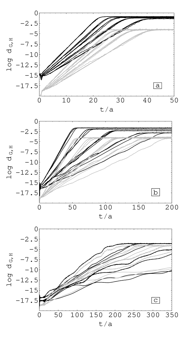
Figure 4: The logarithmic distance evolution in the gauge (black) and Higgs (grey) sectors at fixed Higgs self-coupling $\bar{\kappa}=1$ is plotted for four lattice volumina corresponding to $N=6,10,20$ and $30$. The initial magnetic energy is parametrized by $\delta$. Panel (a) corresponds to $\delta=1.0,0.5,0.45,0.4,0.35$, panel (b) to $\delta=0.3,0.25,0.2,0.15$ and panel (c) to the two smallest values $\delta=0.1,0.05$.

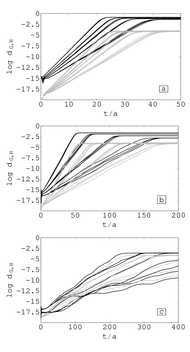
Figure 5: The logarithmic distance evolution in the gauge (black) and Higgs (grey) sectors on a $N=20$ lattice for four different Higgs self-couplings $\bar{\kappa}=1,$ $8,$ $16$ and $24$. The distance trajectories are grouped as in Fig. 4 according to their initial average magnetic energy (parametrized by $\delta$): panel (a) contains the curves corresponding to $\delta=1.0,0.5,0.45,0.4,0.35$, panel (b) corresponds to $\delta=0.3,0.25,0.2,0.15$ and panel (c) to the two smallest values $\delta=0.1,0.05$.

Guided by the above arguments, we generate trajectory pairs for 11 values of $\delta\in\left[0.05,1\right]$. For each of them, we plot the resulting $\ln d{{}_{\text{G}}}\left(t\right)$ (black lines) and $\ln d{{}_{\text{H}}}\left(t\right)$ (grey lines) in Fig. 4 at fixed Higgs self-coupling $\bar{\kappa}=1$ on lattices of four different sizes corresponding to $N=6,10,20$ and $30$, and in Fig. 5 on a $N=20$ lattice with the Higgs coupling values $\bar{\kappa}=1,8,16$ and $24$. (The configuration pair studied in Ref. hei97 on a relatively small lattice with $N=10$ and $\delta=0.2$, $\bar{R}=0.2,$ $\bar{\kappa}=1$ is therefore included in our sample.) The corresponding logarithmic distances $\ln d_{\text{G,H}}\left(t\right)$ for the 11 $\delta$ values are grouped into three sets which are separately plotted in panels (a) – (c) of Figs. 4 and 5: in panel (a) we display $\ln d_{\text{G,H}}$ for the five largest values $\delta=1.0,0.5,0.45,0.4,0.35$, in panel (b) for the values $\delta=0.3,0.25,0.2,0.15$ and in panel (c) for the two smallest values $\delta=0.1,0.05$. All $\delta$ values except for the smallest (i.e. $\delta=0.05$, which is most strongly affected by finite-size artefacts) store more energy in the gauge than in the Higgs sector.

The essential characteristic which all logarithmic distance histories of Figs. 4 and 5 share is that after a latency period of varying length they start to rise at least approximately linearly with $t/a$ before reaching a time-independent saturation plateau (which lies somewhat outside the plotted $\bar{t}$ domain for $\delta=0.05$) at the maximal distance in the compact phase space. Distance saturation at large $\bar{t}=t/a$ is a consequence of the compactness of the lattice gauge group and could be avoided by periodical rescaling (cf. Sec. II.3). The linear regions and the underlying exponential growth rates between initially almost identical field configurations reveal an exponential sensitivity of the distance evolution to the initial conditions, i.e. the standard hallmark of temporal chaos. Not surprisingly, the fields grow apart at a faster pace when their energy increases, i.e. the slopes in Figs. 4 and 5 grow with $\delta$. For each field trajectory, furthermore, the linear regions of both $\ln d{{}_{\text{G}}}\left(t\right)$ and $\ln d{{}_{\text{H}}}\left(t\right)$ have the same average slopes. This result differs from a previous estimate for one trajectory bir96 and will be discussed further in Sec. IV.1. Moreover, for $\delta\lesssim 0.2$ the latency period, which is hardly noticeable for larger $\delta$, expands and the linear growth becomes increasingly modulated by oscillations whose frequency increases with $\delta$. This behavior was observed in YM theory as well and can be traced to the impact of the next-to-maximal Lyapunov exponents which grows when the maximal exponent decreases mul92 . Obviously, these oscillations reduce the accuracy with which the maximal Lyapunov exponent can be determined from the slopes of $\ln d{{}_{\text{G,H}}}\left(t\right)$ in the linear regions (see below).

Figures 4 and 5 further show that for all field trajectories (except that with $\delta=0.05$) $\ln d{{}_{\text{H}}}\left(t\right)$ stays below $\ln d{{}_{\text{G}}}\left(t\right)$. This reflects the smaller amount of energy initially stored in the Higgs sector for $\delta>0.05$ (cf. Sec. III.1) and will change during the long-time evolution to be discussed in Sec. IV.3. In addition, the height of the saturation plateaus of $\ln d_{\text{G}}\left(t\right)$ decreases slightly with $\delta$ while that of $\ln d{{}_{\text{H}}}\left(t\right)$ remains constant. This may indicate that the maximal magnetic gauge-field distance (29) is reached only when sufficient gauge-field energy is available. Apart from these differences in the saturation behavior, however, even the modulation patterns of $\ln d_{\text{G}}\left(t\right)$ and $\ln d{{}_{\text{H}}}\left(t\right)$ are very similar. This suggests that, despite the small gauge-Higgs coupling ensured by Eq. (35), the time dependence of the gauge and Higgs components of at least the most unstable mode has already synchronized after a few lattice time units.

The qualitative dependence of the results on the lattice size, i.e. on $N\in\left\{6,10,20,30\right\}$ with the lattice UV cutoff $a^{-1}$ kept fixed, can be judged by comparing the distance histories in Fig. 4. Figure 4 a contains the results for $1\geq\delta\geq 0.35$. Although the fields are randomly initialized, the curves with identical $\delta$ but different $N$ clearly cluster, i.e. in accord with the bound (39) essentially no finite-size effects can be observed in the covered $N$ and $\delta$ regions (while lattice-spacing effects should become noticeable for $\delta$ close to unity [cf. Eq. (38)]). Indications for a similar $N$ independence were found in pure YM theory mul92 . This may suggest that the most unstable modes, i.e. those which dominantly drive the chaotic time evolution of initially adjacent configurations, have for sufficiently large initial magnetic field energy (corresponding to $\delta\geq 0.35$) typical wavelengths which are small enough to be accommodated by even the largest considered IR cutoff (corresponding to $N=6$), or in other words that these most chaotic modes essentially fit inside a periodic $\left(6a\right)^{3}$ lattice volume. As shown in Figs. 4b and 4c, however, for smaller $\delta\lesssim 0.2$ finite-size corrections become visible in the average slopes of the (increasingly oscillation modulated) linear regions of $\ln d{{}_{\text{G,H}}}\left(t\right)$ and cause them to differ more strongly. A systematic trend in the $N$ dependence of these slopes cannot be discerned in our data, however, whereas in pure YM theory the slope was found to increase on smaller lattices mue96 .

Figure 5 reveals the qualitative dependence of the distance histories on the Higgs self-coupling $\bar{\kappa}$. In the range $\bar{\kappa}\in\left\{1,8,16,24\right\}$ (for $N=20$) it bears several qualitative similarities with the $N$ dependence of Fig. 4. To begin with, a $\bar{\kappa}$ dependence is hardly noticeable for large $\delta$ while the slope of the linear regions becomes increasingly $\bar{\kappa}$ dependent towards smaller values of $\delta$, although again without a perceivable systematic trend. The, as a whole, only mild sensitivity of the slopes to $\bar{\kappa}$ is probably a consequence of the fact that even $\ln d_{\text{H}}\left(t\right)$ is mainly determined by the most unstable gauge-field fluctuations and hence relatively insensitive to the self-interactions of the Higgs field. After full equilibration between the gauge and Higgs sector has taken place, the $\bar{\kappa}$ dependence of the slopes may therefore be systematically enhanced (if distance saturation is avoided by periodical rescaling), as we will indeed find in Sec. IV.3. Since a more strongly self-coupled Higgs sector would absorb energy from the gauge sector (in which for $\delta\geq 0.1$ more initial energy is stored, cf. Sec. III.1) faster, it should similarly increase the $\bar{\kappa}$ dependence of the slopes.

To summarize, all members of the representative set of distance histories (in the weakly coupled, symmetric YMH phase) discussed above increase exponentially and thereby exhibit chaotic behavior. For $\delta\gtrsim 0.3$ the $\ln d_{\text{G,H}}\left(t\right)$ become practically independent of the Higgs coupling $\bar{\kappa}$ and (for $N\geq 6$) of the lattice volume.

IV Lyapunov exponents, scaling behavior and damping rates

In the following section we proceed to the quantitative evaluation of the maximal Lyapunov exponents for randomized and coherent initial conditions, and we discuss their energy dependence and relation to the plasmon damping rates.

IV.1 Maximal Lyapunov exponents of randomly initialized fields

The analysis of the last section showed that all our 77 randomly initialized field pairs belong to the chaotic part of the YMH phase space. This suggests that in the unbroken phase of YMH theory chaotic behavior is either universal (i.e. exists for all energies) or at least prevalent in most of the weakly coupled phase space . In order to quantify this behavior, we will now evaluate the classic measure for the chaoticity of a dynamical system, i.e. the maximal Lyapunov exponent $\lambda$ or equivalently the exponential growth rate of the distance between initially neighboring dynamical variables. We are going to extract the MLEs from the numerical results of Sec. II.3 by averaging the time histories $d_{\text{G}}\left(\bar{E},\bar{\kappa},N;t\right)$ and $d_{\text{H}}\left(\bar{E},\bar{\kappa},N;t\right)$ of the gauge and Higgs field distance measures over the time interval $\Delta$ during which they remain in the linear regime, i.e.

$$\lambda_{\text{G},\text{H}}\left(\bar{E},\bar{\kappa},N\right)=\left\langle\frac{d}{dt}\ln\frac{d_{\text{G,H}}\left(\bar{E},\bar{\kappa},N;t\right)}{d_{\text{G,H}}\left(\bar{E},\bar{\kappa},N;0\right)}\right\rangle_{\Delta}.$$ (40)

Note that we have replaced the dependence on the initialization parameter $\delta$ with that on the total (dimensionless) energy $\bar{E}$ of the YMH system, and that we suppressed the dependence on the remaining initialization parameter, the Higgs amplitude $\bar{R}$, which is kept at the same value for all our trajectories (cf. Sec. III.1). We further recall that the above method for obtaining the MLEs becomes increasingly error-prone towards lower energies where equilibration proceeds more slowly while the impact of the next-to-maximal Lyapunov exponents grows and generates modulations of $\ln d_{\text{G,H}}\left(t\right)$ with decreasing frequency. Similar problems were encountered in Ref. mul92 and will be tamed below by periodically rescaling the distance measures (cf. Sec. IV.3).

Our numerical results for the dimensionless MLEs $\bar{\lambda}_{\text{G},\text{H}}\left(\bar{E},\bar{\kappa},N\right):=a\lambda_{\text{G},\text{H}}\left(\bar{E},\bar{\kappa},N\right)$, based on the 77 field-pair evolution histories of Sec. III.3, are collected in Table 1.

	$N=6$ $\bar{\kappa}=1$	$N=10$ $\bar{\kappa}=1$	$N=20$ $\bar{\kappa}=1$	$N=30$ $\bar{\kappa}=1$	$N=20$ $\bar{\kappa}=8$	$N=20$ $\bar{\kappa}=16$	$N=20$ $\bar{\kappa}=24$
$\bar{E}=0.04374$	$0.06507$ $0.07521$	$0.07445$ $0.07900$	$0.06179$ $0.06799$	$0.04563$ $0.04713$	$0.06276$ $0.06422$	$0.02922$ $0.02517$	$0.04862$ $0.04712$
$\bar{E}=0.10076$	$0.07394$ $0.07343$	$0.05838$ $0.05820$	$0.05052$ $0.05004$	$0.05617$ $0.05633$	$0.05246$ $0.05270$	$0.05981$ $0.06028$	$0.03972$ $0.03997$
$\bar{E}=0.19028$	$0.09117$ $0.09156$	$0.07269$ $0.07320$	$0.09783$ $0.09833$	$0.09281$ $0.09336$	$0.08522$ $0.08561$	$0.09264$ $0.09330$	$0.08767$ $0.08849$
$\bar{E}=0.30482$	$0.13357$ $0.13349$	$0.13348$ $0.13410$	$0.13017$ $0.13075$	$0.13751$ $0.13803$	$0.13876$ $0.13888$	$0.13665$ $0.13655$	$0.13435$ $0.13394$
$\bar{E}=0.43527$	$0.19660$ $0.19844$	$0.20009$ $0.20126$	$0.20985$ $0.21099$	$0.20906$ $0.21011$	$0.22112$ $0.22164$	$0.20315$ $0.20313$	$0.20032$ $0.19922$
$\bar{E}=0.57202$	$0.28580$ $0.28877$	$0.25783$ $0.25994$	$0.29550$ $0.29795$	$0.29339$ $0.29540$	$0.28875$ $0.29021$	$0.28975$ $0.29024$	$0.29050$ $0.28895$
$\bar{E}=0.70604$	$0.36801$ $0.37857$	$0.39740$ $0.39802$	$0.39422$ $0.39841$	$0.39359$ $0.39638$	$0.39232$ $0.39354$	$0.37328$ $0.37355$	$0.38446$ $0.38460$
$\bar{E}=0.82974$	$0.46159$ $0.46487$	$0.46709$ $0.47145$	$0.48083$ $0.48596$	$0.46971$ $0.47334$	$0.47193$ $0.47344$	$0.47730$ $0.47800$	$0.48521$ $0.48630$
$\bar{E}=0.93767$	$0.50948$ $0.51818$	$0.53934$ $0.53885$	$0.53530$ $0.53656$	$0.54047$ $0.54306$	$0.52785$ $0.52760$	$0.53862$ $0.53854$	$0.54295$ $0.54123$
$\bar{E}=1.02672$	$0.56526$ $0.56125$	$0.56621$ $0.56722$	$0.58570$ $0.58918$	$0.58284$ $0.58643$	$0.57729$ $0.57799$	$0.58613$ $0.58700$	$0.57540$ $0.57636$
$\bar{E}=1.22634$	$0.63279$ $0.64082$	$0.65405$ $0.65811$	$0.65635$ $0.65997$	$0.65077$ $0.65550$	$0.64431$ $0.64588$	$0.65041$ $0.65104$	$0.64915$ $0.65008$

Table 1: Maximal Lyapunov exponents $\bar{\lambda}_{\text{G}}=a\lambda_{\text{G}}$ (upper entries) and $\bar{\lambda}_{\text{H}}=a\lambda_{\text{H}}$ (lower entries) as a function of total energy $\bar{E}=g^{2}Ea$, Higgs self-coupling $\bar{\kappa}$ and number $N$ of lattice sites per dimension.

A first glance at the table confirms the qualitative trends which we noticed in our discussion of Figs. 4 and 5 in Sec. III.3. Besides the expected increase of the $\bar{\lambda}_{\text{G},\text{H}}$ with $\bar{E}$ (or $\delta$), which we will analyze quantitatively in Sec. IV.2, the data show fluctuations in the statistically expected range of about 10% for different Higgs self-couplings and lattice sizes, but except for the smallest $\bar{E}$ no obvious systematic dependence on either $\bar{\kappa}$ or $N$. At the considered intermediate times (i.e. after separate preequilibration of gauge and Higgs sectors but before their mutual thermalization is complete) and at least at intermediate energies $\bar{E}$ or $\bar{E}_{\text{p}}$ systematic finite-size and lattice-spacing effects are therefore small. Furthermore, the above results indicate that the Higgs sector plays a rather minor role in the chaoticity of the full YMH system, at least at the weak couplings which the initial conditions of Sec. III.1 implement. The most unstable mode, which in large part drives the chaotic behavior, should therefore be controlled mainly by the gauge dynamics. As a consequence, reasonable estimates for the MLEs can be extracted at the preequilibration stage and the MLE values of the SU$\left(2\right)$ YMH system should be similar to those of pure SU$\left(2\right)$ YM theory mul92 ; mue96 , which is confirmed by the results in Table 1.

While we find the Higgs sector to have only limited impact on the chaotic YMH dynamics in the weakly coupled symmetric phase, it may be useful to recall the results of Refs. mat81 ; ber85 in the homogeneous limit, i.e. for wavelengths much larger than the inverse amplitudes $\left|A\right|^{-1},\left|\phi\right|^{-1}$, which reveal a more dramatic role of the Higgs field in the broken phase (even at nonzero Weinberg angle). This is a consequence of the dynamically generated gauge-field mass in the broken phase which is known to damp (and beyond a critical value to fully suppress) chaotic behavior bir94 . (We note in passing that chaos is not only damped by gauge-field masses generated via spontaneous symmetry breaking, but also by those due to quantum fluctuations according to the Coleman-Weinberg mechanism mat97 , topological excitations, polarization of the heat bath at finite temperature, and external charges bir294 .) In Ref. ber85 chaotic behavior was observed only beyond the threshold energy $\bar{E}_{\text{th}}\simeq 0.3$ (showing that chaos is not universal in the broken phase), and for the energy $\bar{E}=5.07\gg\bar{E}_{\text{th}}$ the MLE was found to be $\bar{\lambda}\simeq 0.25$ ber85 , i.e. an order of magnitude smaller than our value $\bar{\lambda}\simeq 2.75$ in the unbroken phase (which we linearly extrapolate [cf. Sec. IV.2] from the values in Table 1 up to $\bar{E}=5.07$). Since constant fields with their few degrees of freedom can exhibit stronger chaoticity and thus produce larger MLEs than our randomized initial configurations, this comparison gives a quantitative idea of how much the chaotic YMH instability is damped by the Higgs mechanism in the broken phase.

Another issue which can be addressed quantitatively on the basis of the data in Table 1 is the relation between the maximal Lyapunov exponents $\bar{\lambda}_{\text{G}}$ and $\bar{\lambda}_{\text{H}}$, which are obtained from the gauge and Higgs field distance measures (29) and (30), respectively. This relation was subject to some debate, in particular at strong coupling bir96 ; hei97 . After an exploratory study in Ref. bir94 , Ref. bir96 provided a first lattice estimate for YMH theory. The $\bar{\lambda}_{\text{H}}$ extracted from the growth rate of the Higgs field distance measure was found to become smaller than $\bar{\lambda}_{\text{G}}$ when the Higgs self-coupling $\bar{\kappa}$ increases. At $\bar{\kappa}=24$ and for $N=10$, in particular, $\bar{\lambda}_{\text{H}}$ was estimated in Ref. bir96 to be about 15% smaller than $\bar{\lambda}_{\text{G}}$. Comparison with the static gauge and Higgs boson damping rate in (resummed) thermal perturbation theory then cast doubt on their relation to the same $\bar{\lambda}_{\text{G}}$ and led to the speculation that the Higgs damping rate may instead be related to $\bar{\lambda}_{\text{H}}$ bir96 . These ideas were later questioned in Ref. hei97 whose improved calculation found $\bar{\lambda}_{\text{G}}$ and $\bar{\lambda}_{\text{H}}$ to agree, although only for one trajectory pair at fixed energy and $\delta=0.2,$ $\bar{\kappa}=1,$ $\bar{R}=0.2$ and $N=10$.

In our case, the $\bar{\lambda}_{\text{G}}$ (upper entries) and $\bar{\lambda}_{\text{H}}$ (lower entries) values in Table 1 agree within errors (at the percent level) in all of the covered YMH phase space, with the deviations slightly decreasing for increasing $\bar{E}$ and $\bar{\kappa}$. Our results therefore show that the finding of Ref. hei97 was not an accidental outcome of one specific initialization choice but that indeed

$$\bar{\lambda}_{\text{G}}\left(\bar{E},\bar{\kappa},N\right)\simeq\bar{\lambda}_{\text{H}}\left(\bar{E},\bar{\kappa},N\right).$$ (41)

Since the individual relaxation times $\tau$ of the gauge and Higgs sectors are set by the inverse MLEs, i.e. $\tau_{\text{G,H}}\simeq\lambda_{\text{G,H}}^{-1}$, Eq (41) naturally explains the observation $\tau_{\text{G}}\sim\tau_{\text{H}}$ in Sec. III.2, i.e. the fact that both gauge and Higgs sectors (separately) self-thermalize over about the same relaxation time. Equation (41) further squares with the general expectation that the maximally unstable field mode of a dynamical system, i.e. the mode associated with the MLE, dominates the exponential distance growth. Hence the MLEs should be independent of the metric used to extract them (modulo constant factors which depend on the field powers involved in the definition of the metric). A possible exception to this rule may arise, however, if the distance measure is blind to the maximally unstable eigenmode. In Ref. hei97 it was argued that such a situation occurs in YMH theory at large coupling $\bar{\kappa}$, where the quartic Higgs self-interaction dominates the potential Higgs energy (12): the amplitude $R_{x}$ then remains practically unchanged during time evolution and decouples from the maximally unstable gauge-field mode to which the Higgs distance measure (30) consequently becomes insensitive. At the still relatively weak coupling $\bar{\kappa}=24$, and the energy $\bar{E}\sim 0.8$ of Ref. bir96 where $d_{\text{H}}\left(t\right)$ is rather strongly time dependent [cf. Fig. 5(a)], however, our results for $\bar{\lambda}_{\text{H}}$ and $\bar{\lambda}_{\text{G}}$ differ by only about 1%. This suggests that the 15% deviation found in Ref. bir96 should mainly be attributed to numerical uncertainties.

IV.2 Energy dependence and relation to plasmon damping rate

As already mentioned, the dependence of the MLEs on the gauge-field energy per degree of freedom, $E_{\text{G}}=E_{\text{p}}/2$ (cf. Eq. (36)), and on the total energy $E$ of the YMH system is a particularly important issue. In pure SU$\left(2\right)$ mul92 ; bir94 and SU$\left(3\right)$ bir94 ; gon93 Yang-Mills theory (whose scaling properties imply that the dimensionless Lyapunov exponent $\bar{\lambda}=\lambda a$ can only depend on $\bar{E}_{\text{p}}=g^{2}aE_{\text{p}}$), the approximately linear relation

$$\lambda_{N_{c}}\simeq c_{N_{c}}g^{2}E_{\text{p}}$$ (42)

with $c_{2}\simeq 0.17$ and $c_{3}\simeq 0.10$ was established numerically in the weak-coupling regime. (An improved SU$\left(2\right)$ analysis and a careful discussion of the involved errors mue96 , triggered by questions raised in Ref. nie96 , later confirmed the results of Refs. mul92 ; bir94 .) The empirical relation (42) helps to clarify the physical role of the MLEs in hot quantum gauge theory. Since the Lyapunov exponents were extracted at times $t\gg\tau_{\text{G}}\simeq\lambda^{-1}$, i.e. after the gauge sector has preequilibrated , the thermal gauge-field ensemble has according to Eq. (37) reached the temperature $T_{\text{G}}=E_{\text{p}}/2$ (at sufficiently large average plaquette energy $E_{\text{p}}$). Together with Eq. (42) this implies the linear relationship $\lambda_{N_{c}}=\tilde{c}_{N_{c}}T_{\text{G}}$, and comparison with the static plasmon damping rate $\gamma_{0,N_{c}}$ of hot quantum SU$\left(N_{c}\right)$ YM theory, as calculated to leading order in hard-thermal-loop resummed perturbation theory bra90 , then revealed the at first rather unexpected relation mul92 ; bir94 ; gon93

$$\lambda_{N_{c}}\simeq 2\gamma_{0,N_{c}}$$ (43)

for $N_{c}=2,3$. [The factor of 2 arises because the growth rate of the distance (29) is twice that of the distance between the gauge fields.] Subsequently, Eq. (43) has been derived under a few heuristic assumptions (in particular on the ergodicity of the gauge-field evolution) in Ref. bir95 .

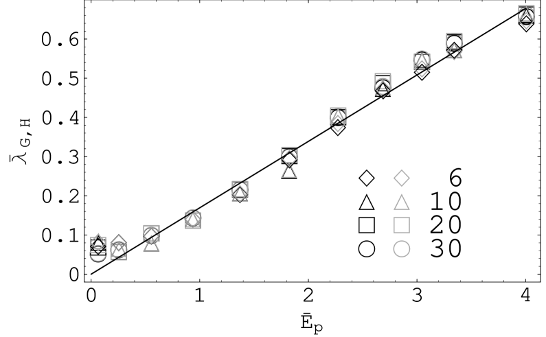
Figure 6: Values of the maximal Lyapunov exponents $\bar{\lambda}_{\text{G}}$ (black symbols) and $\bar{\lambda}_{\text{H}}$ (grey symbols) as a function of the average energy per plaquette $\bar{E}_{\text{p}}$ for $\bar{\kappa}=1$ and $N=6,10,20,30$.

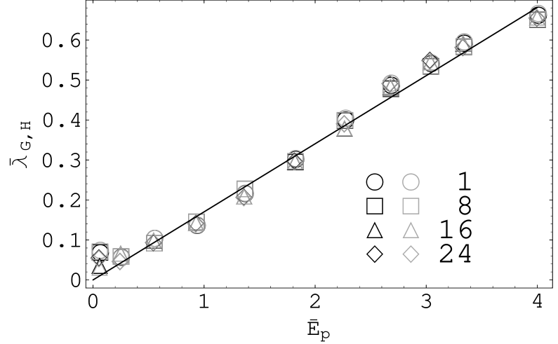
Figure 7: Values of the maximal Lyapunov exponents $\bar{\lambda}_{\text{G}}$ (black symbols) and $\bar{\lambda}_{\text{H}}$ (grey symbols) as a function of the average energy per plaquette $\bar{E}_{\text{p}}$ for $N=20$ and $\bar{\kappa}=1,8,16,24$.

On the basis of the rather exhaustive data set in Table 1, we are now able to address the analogous question of how the MLEs are related to the average plaquette and total energies in the weak-coupling regime of YMH theory. In Fig. 6 we plot the MLEs for $\bar{\kappa}=1$ on lattices with $N\in\left\{6,10,20,30\right\}$ (corresponding to the first four columns of Table 1) in the full range of average plaquette energies $0\lesssim ag^{2}E_{\text{p}}\equiv\bar{E}_{\text{p}}\lesssim 4$. Figure 7 contains all remaining MLEs of Table 1, i.e. those for $\bar{\kappa}=\left\{1,8,16,24\right\}$ at $N=20$. The straight lines also drawn in Figs. 6 and 7 are the best linear fits to the data:

$$\bar{\lambda}_{\text{G,H}}\left(E_{\text{p}}\right)\simeq 0.17ag^{2}E_{\text{p}}\simeq\frac{1}{6}\bar{E}_{\text{p}}.$$ (44)

The figures show that the MLEs indeed depend within errors linearly on the average energy $E_{\text{p}}$ per plaquette, as in YM theory. In fact, the linearity of $\bar{\lambda}\left(\bar{E}_{\text{p}}\right)$ seems to be a nontrivial consequence of the non-Abelian nature of the gauge group. (The MLEs of scalar $\phi^{4}$ theory and Abelian U$\left(1\right)$ gauge theory, in contrast, were found to vanish in the continuum limit $a\rightarrow 0$ bir94 .) Remarkably, even the slope of the linear relation (44) is almost identical to that in SU$\left(2\right)$ Yang-Mills theory mul92 ; bir94 ; mue96 . (It is also consistent with the value of the ratio $\bar{\lambda}/\bar{E}_{\text{p}}$ which was extracted from the trajectory with $\delta=0.2,$ $\bar{\kappa}=1,$ $\bar{R}=0.2$ and $N=10$ in Ref. hei97 .)

Equation (44) implies that for identical gauge field energy the MLEs of YM and YMH theory are approximately equal. This provides our main evidence for the maximally unstable YMH mode to belong primarily to the gauge sector, and suggests that the chaoticity and equilibration properties of the Higgs sector are mediated by this gauge-field mode as well (at least at weak coupling and if the major part of the initial energy is stored in the gauge sector). It also makes it more plausible that the MLEs of YMH theory are related to the gauge field damping rates bir94 ; hei97 . Furthermore, it is consistent with the approximately equal relaxation times $\tau_{\text{G}}\sim\tau_{\text{H}}$ (cf. Sec. III.2) and exponential distance growth rates, cf. Eq. (41), in the gauge and Higgs sectors.

Nonetheless, the plaquette energy dependence of the MLEs in Figs. 6 and 7 also shows small systematic deviations from linearity which become most notable towards the lowest $\bar{E}_{\text{p}}$ values. The same effect was observed in pure Yang-Mills theory mue96 , and a glance at the criterion (39) indicates that finite-size errors are responsible for the systematic upward trend of the MLEs at the smallest $\bar{E}_{\text{p}}$. In fact, this is what one would intuitively expect since field modes with longer average wavelengths are more strongly deformed by the periodic boundary conditions. The slopes of the logarithmic distance histories become most strongly modulated towards smaller $\bar{E}_{\text{p}}$ (cf. Sec. III.3), furthermore, which introduces additional systematic errors. Together with the finite-time errors to be discussed in Sec. IV.3 they might cause additional deviations from a linear energy dependence of the MLEs. Towards the maximal value $\bar{E}_{\text{p}}=4$ of the average energy per plaquette, on the other hand, lattice spacing [cf. Eq. (38)] and compact phase-space artefacts are likely to affect the results nie96 ; kra96 .

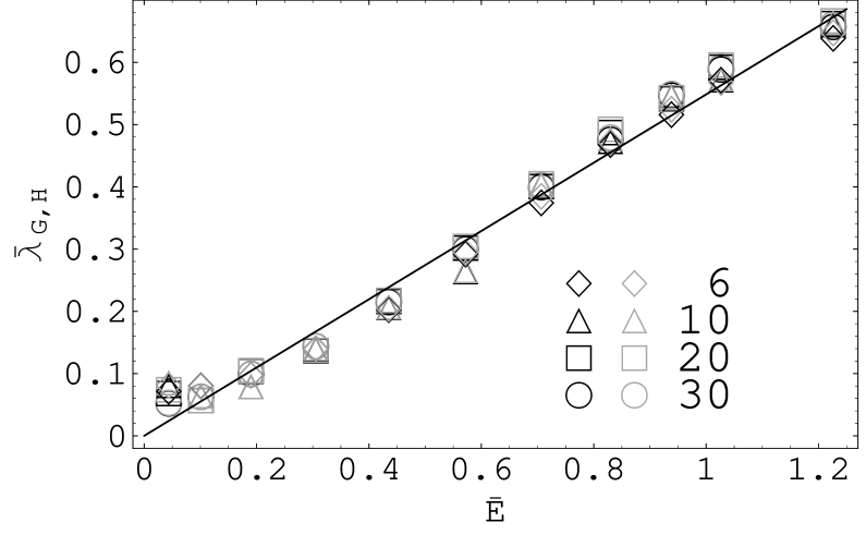
Figure 8: Values of the maximal Lyapunov exponents $\bar{\lambda}_{\text{G}}$ (black symbols) and $\bar{\lambda}_{\text{H}}$ (grey symbols) as a function of the total energy $\bar{E}$ for $\bar{\kappa}=1$ and $N=6,10,20,30$.

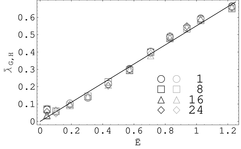
Figure 9: Values of the maximal Lyapunov exponents $\bar{\lambda}_{\text{G}}$ (black symbols) and $\bar{\lambda}_{\text{H}}$ (grey symbols) as a function of the total energy $\bar{E}$ for $N=20$ and $\bar{\kappa}=1,8,16,24$.

Since the YMH system has a second characteristic energy scale besides $\bar{E}_{\text{p}}$, i.e. the total energy $\bar{E}$ which additionally includes both the energy stored in the Higgs field and in the gauge-Higgs interactions (cf. Sec. III.2) and is strictly conserved at all times, it is natural to ask how the MLEs depend on $\bar{E}$. In order to answer this question, we plot our MLEs in Figs. 8 and 9 as a function of $\bar{E}$ (for the same $\bar{\kappa}$ and $N$ values as in Figs. 6 and 7) and find the dependence on the total YMH energy to be approximately linear as well:

$$\bar{\lambda}_{\text{G},\text{H}}\left(\bar{E}\right)\simeq 0.55\bar{E}.$$ (45)

The above scaling behavior can be understood by recalling that our MLEs were extracted during evolution times $t/a\leq 400$ over which the distances generally saturate, but before the gauge and Higgs fields have started to exchange appreciable amounts of energy. A glance at Fig. 2 shows that after the gauge and Higgs sector have separately preequilibrated (i.e. for $t/a\gg\bar{\lambda}^{-1}$), $\bar{E}_{\text{G}}=\bar{E}_{\text{p}}/2$ and $\bar{E}_{\text{H}}$ are practically time-independent in this phase. Moreover, as mentioned in Sec. III.3, staying in the weak-coupling regime requires initial conditions which (except for the smallest $\delta=0.05\,$) store considerably more energy in the gauge than in the Higgs sector (cf. e.g. Fig. 2 which corresponds to $\delta=0.2$). In this situation one derives from the definition of $\bar{E}$ in Sec. III.2, which implies $\bar{E}_{\text{p}}=-4\bar{E}_{\text{H}}/3+10\bar{E}/3$, and from Eq. (44) that

$$\bar{\lambda}_{\text{G,H}}\left(\bar{E},\bar{E}_{\text{H}}\right)\simeq-\frac{2}{9}\bar{E}_{\text{H}}+\frac{5}{9}\bar{E}\overset{\bar{E}_{\text{H}}\ll\bar{E}}{\longrightarrow}\frac{5}{9}\bar{E},$$ (46)

which explains the linear behavior and numerical slope of Eq. (45). [Eq. (46) also explains the numerical scaling relation $\bar{\lambda}_{\text{G}}\left(\bar{E}\right)\simeq 0.53\bar{E}$ ful01 for SU$\left(2\right)$ YM theory where $\bar{E}_{\text{H}}\equiv 0$.] We reemphasize that these results hold for MLEs extracted in the time window $\bar{\lambda}^{-1}\ll t/a\leq 400$ during which $\bar{E}_{\text{G}}$ and $\bar{E}_{\text{H}}\ll\bar{E}_{\text{G}}$ remain practically constant.

IV.3 Long-time evolution of the Lyapunov histories

At later times the Higgs sector will pick up energy from the gauge sector, i.e. $\bar{E}_{\text{p}}$ will drop (for $\delta>0.05\,$) while $\bar{E}$ remains constant (cf. Figs. 2 and 3). In the $t\rightarrow\infty$ limit the MLEs must attain a constant value, as implied in their formal definition, and so will $\bar{E}_{\text{p}}$. This saturation is strongly delayed, however, by the exceptionally long relaxation times which govern the equilibration between the gauge and Higgs fields. In the remainder of this section we will analyze the quantitative impact of this saturation behavior on the extracted MLE values. To this end, we compute the “Lyapunov histories”

$$\bar{\lambda}_{\text{G,H}}\left(\bar{E},\bar{\kappa},N;t\right):=\frac{a}{t}\ln\frac{\tilde{d}_{\text{G,H}}^{\left(\text{alt}\right)}\left(\bar{E},\bar{\kappa},N;t\right)}{\tilde{d}_{\text{G,H}}^{\left(\text{alt}\right)}\left(\bar{E},\bar{\kappa},N;0\right)}=\frac{a}{t}\sum_{k=1}^{t/\tau}\ln s_{k}\overset{t\rightarrow\infty}{\longrightarrow}\bar{\lambda}_{\text{G,H}}\left(\bar{E},\bar{\kappa},N\right)$$ (47)

[where $\tilde{d}_{\text{G,H}}^{\left(\text{alt}\right)}$ are the rescaled distances (31) and (32), and the $s_{k}$ are the rescaling factors obtained after the $k$-th scaling step with rescaling period $\tau$], which approach the exact MLEs in the $t\rightarrow\infty$ limit, for eight long-time field-pair trajectories in the time interval $t/a\in\left[0,20000\right]$ on an $N=10$ lattice. (In order to improve numerical efficiency, we increase the rescaling period $\tau$ with increasing saturation time, i.e. with decreasing $\delta$, as detailed in the figure captions below.)

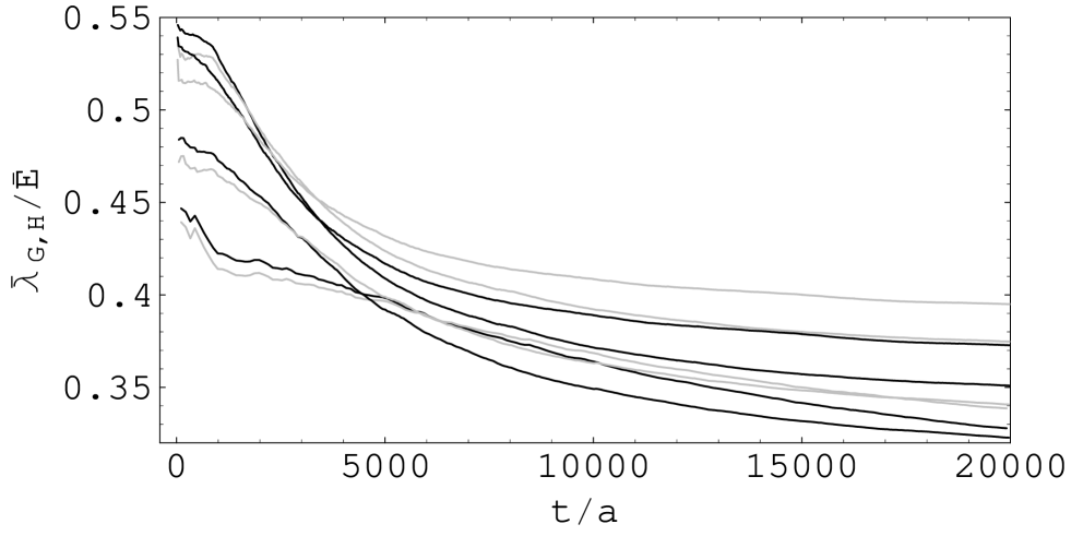
Figure 10: Long-time evolution of the Lyapunov histories $\bar{\lambda}_{\text{G}}\left(t\right)/\bar{E}$ (black lines) and $\bar{\lambda}_{\text{H}}\left(t\right)/\bar{E}$ (grey lines) for $\left(\delta,\tau\right)=\left(0.6,25\right)$ (2nd largest initial values), $\left(0.45,30\right)$ (largest initial values), $\left(0.3,55\right)$ (2nd lowest initial values) and $\left(0.2,110\right)$ (lowest initial values) (with $\Delta t=0.0005,$ $\bar{\kappa}=1,$ $\bar{R}=0.2$ and $N=10$).

In Fig. 10 we show the Lyapunov histories $\bar{\lambda}_{\text{G}}\left(t\right)/\bar{E}$ (black lines) and $\bar{\lambda}_{\text{H}}\left(t\right)/\bar{E}$ (grey lines), “normalized” by the total energy, for the four long-time field-pair histories with $\bar{\kappa}=1$ and initial magnetic energies specified by $\delta=0.2,0.3,0.45$ and $0.6$. (This corresponds to approximately equally spaced $\bar{E}_{\text{p}}$ values, cf. Figure 1.) A first important characteristic of all Lyapunov histories is their monotonic decrease with time. Moreover, the saturation of $\bar{\lambda}_{\text{G}}\left(t\right)$ for large $t$ can be seen to proceed very slowly: especially for smaller $\delta$ it is not fully completed even at $t=2\times 10^{4}a$. In all four cases, furthermore, $\bar{\lambda}_{\text{G}}\left(t\right)$ starts out somewhat larger than $\bar{\lambda}_{\text{H}}\left(t\right)$ but becomes smaller when the gauge and Higgs sectors start to exchange substantial amounts of energy. The deviations between $\bar{\lambda}_{\text{G}}\left(t\right)$ and $\bar{\lambda}_{\text{H}}\left(t\right)$ remain at the one-percent level during the initial time evolution (as reflected in the $\bar{\lambda}_{\text{G}}$ and $\bar{\lambda}_{\text{H}}$ estimates of Table 1) and increase systematically up to 5% at $t=20000a$. Hence $\bar{\lambda}_{\text{G}}\left(t\right)$ and $\bar{\lambda}_{\text{H}}\left(t\right)$ remain approximately equal over the whole time evolution until they turn into the MLEs for $t\rightarrow\infty$.

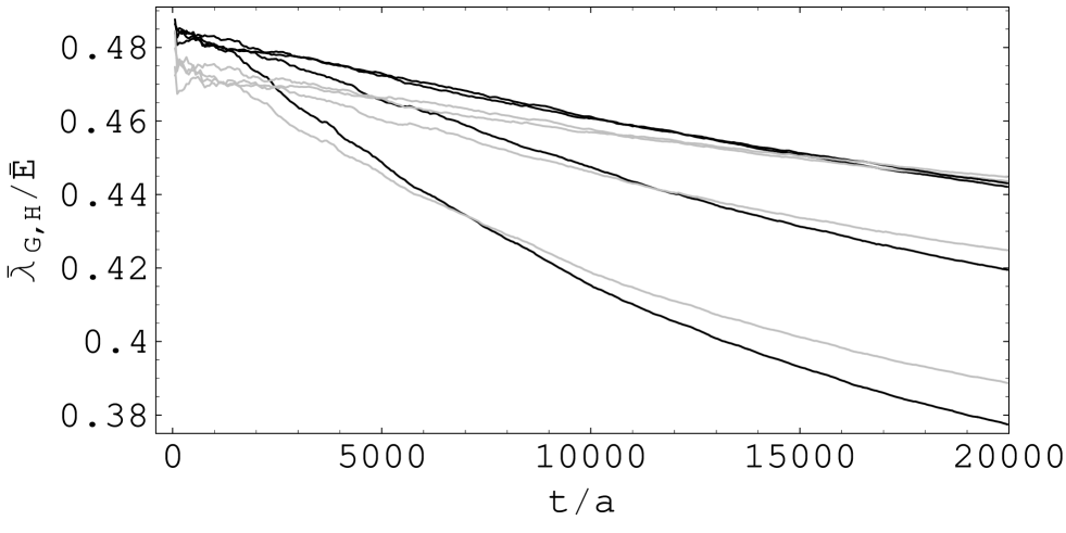
Figure 11: Long-time evolution of the Lyapunov histories $\bar{\lambda}_{\text{G}}\left(t\right)/\bar{E}$ (black lines) and $\bar{\lambda}_{\text{H}}\left(t\right)/\bar{E}$ (grey lines) for $\bar{\kappa}=8,$ $16,$ $24$ (from bottom to top) with $\Delta t=0.001$. The uppermost curve, overlapping with its larger time-step counterpart, is for $\bar{\kappa}=24$ with $\Delta t=0.0005$. (All curves correspond to $\delta=0.3,\tau=55,$ $\bar{R}=0.2$ and $N=10$).

In Fig. 11 we display the Lyapunov histories $\bar{\lambda}_{\text{G,H}}\left(t\right)/\bar{E}$ for an intermediate $\delta=0.3$ and the four values $\bar{\kappa}=8,16,24$ of the Higgs self-coupling. The main tendencies observed in Fig. 10 remain intact for larger $\bar{\kappa}$, although increasing Higgs couplings further delay the saturation of the Lyapunov histories. Indeed, already for $\bar{\kappa}=8$ it is more difficult to reliably extrapolate $\bar{\lambda}_{\text{G,H}}\left(t\right)$ from the simulation interval $t/a\in\left[0,20000\right]$ to the MLE value at $t\rightarrow\infty$. On the other hand, larger $\bar{\kappa}$ values further reduce the deviations between $\bar{\lambda}_{\text{G}}\left(t\right)$ and $\bar{\lambda}_{\text{H}}\left(t\right)$ (which suggests that the opposite tendency observed in Ref. bir96 was due to a numerical artefact), and they also reduce the long-time variations of $\bar{\lambda}_{\text{G,H}}\left(t\right)/\bar{E}$ and hence the finite-time errors of the MLEs.

In order to check whether the used integration time step $\Delta t=0.001$ is small enough, we have also performed a simulation with half of its value for $\bar{\kappa}=24$. The corresponding curve, also drawn in Fig. 11, is essentially identical to the one with the larger time step, which shows that the latter has no relevant time discretization error. Finally, we note that when the Lyapunov histories decrease during equilibration, one may expect their sensitivity to the Higgs sector to become larger. Figure 11 shows that their dependence on the Higgs self-coupling $\bar{\kappa}$ is negligible at smaller evolution times ($t\lesssim 2000a$), as manifest in Table 1, but indeed becomes more pronounced for larger $t$.

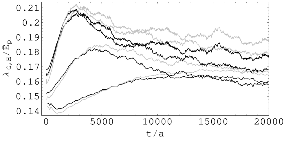
Figure 12: Long-time evolution of the Lyapunov histories $\bar{\lambda}_{\text{G}}\left(t\right)/\bar{E}_{\text{p}}$ (black lines) and $\bar{\lambda}_{\text{H}}\left(t\right)/\bar{E}_{\text{p}}$ (grey lines) for $\delta=0.6$ (largest starting values), 0.45, 0.3 and $0.2$ (lowest starting values) (with $\bar{\kappa}=1$ and $N=10$).

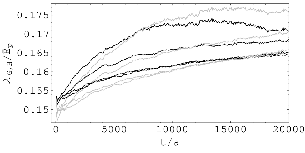
Figure 13: Long-time evolution of the Lyapunov histories $\bar{\lambda}_{\text{G}}\left(t\right)/\bar{E}_{\text{p}}$ (black lines) and $\bar{\lambda}_{\text{H}}\left(t\right)/\bar{E}_{\text{p}}$ (grey lines) for $\bar{\kappa}=8,$ $16,$ $24$ and $\Delta t=0.001$ (from top to bottom) and $\bar{\kappa}=24$ with $\Delta t=0.0005$ ($\delta=0.3,\tau=55,$ $\bar{R}=0.2$ and $N=10$).

We now turn to the examination of the ratios $\bar{\lambda}_{\text{G}}\left(t\right)/\bar{E}_{\text{p}}\left(t\right)$ and $\bar{\lambda}_{\text{H}}\left(t\right)/\bar{E}_{\text{p}}\left(t\right)$ which we plot in Figs. 12 and 13 for the same parameter values as in Figs. 10 and 11. The closely parallel movement of $\bar{\lambda}_{\text{G}}\left(t\right)$ and $\bar{\lambda}_{\text{H}}\left(t\right)$, and the systematics of their small deviations remain visible here as well. The initial drop in $\bar{\lambda}_{\text{G,H}}\left(t\right)/\bar{E}_{\text{p}}\left(t\right)$ (in particular for $\delta=0.2$) falls into the time period during which $\bar{E}_{\text{p}}\left(t\right)$ is practically constant, i.e. it is caused by the decrease of $\bar{\lambda}_{\text{G}}\left(t\right)$. Later on the gauge-field energy $\bar{E}_{\text{p}}\left(t\right)$ starts to drop (cf. Fig. 2) and overcompensates the continuing decrease of $\bar{\lambda}_{\text{G,H}}\left(t\right)$. This causes the ratios $\bar{\lambda}_{\text{G,H}}\left(t\right)/\bar{E}_{\text{p}}\left(t\right)$ to rise. For $\delta=0.2$, one furthermore finds from (slightly extrapolating) Fig. 2 that $\bar{E}_{\text{p}}\left(t\right)=2\bar{E}_{\text{G}}\left(t\right)\rightarrow 2\bar{E}$ for $t\gtrsim 13000a$, so that the continuing, slight decrease of

$$\frac{\bar{\lambda}_{\text{G,H}}\left(t\right)}{\bar{E}_{\text{p}}\left(t\right)}\overset{t/a\gtrsim 13000,\text{ }\delta=0.2}{\longrightarrow}\frac{1}{2\bar{E}}\bar{\lambda}_{\text{G,H}}\left(t\right)$$ (48)

for $t\gtrsim 13000a$ has again to be attributed solely to the behavior of $\bar{\lambda}_{\text{G,H}}\left(t\right)$. An important result, visible in both Figs. 12 and 13, is that the ratios $\bar{\lambda}_{\text{G,H}}\left(t\right)/\bar{E}_{\text{p}}\left(t\right)$ saturate significantly earlier than $\bar{\lambda}_{\text{G,H}}\left(t\right)/\bar{E}$ even at larger values of $\bar{\kappa}$. [Short-time fluctuations of the average plaquette energy $\bar{E}_{\text{p}}\left(t\right)$ cause the time evolution of $\bar{\lambda}_{\text{G,H}}\left(t\right)/\bar{E}_{\text{p}}\left(t\right)$ to appear more ragged.] This indicates that for large $t$, i.e. on the approach to full equilibrium, the average gauge energy $\bar{E}_{\text{p}}\left(t\right)/2$ decreases at the same rate as $\bar{\lambda}_{\text{G,H}}\left(t\right)$.

As already alluded to, our long-time evolution results allow for a quantitative assessment of the finite-time errors in the MLE estimates of Table 1, which were extracted at rather short evolution times. Figure 10 indicates that for $\bar{\kappa}=1$ the time variations of $\bar{\lambda}_{\text{G}}\left(t\right)$ reach about 25% for $\delta=0.2$ and about 30% for $\delta=0.6$, while they remain about 5% smaller for the corresponding $\bar{\lambda}_{\text{H}}\left(t\right)$. These variations may be considered as a (conservative) upper bound on the systematic finite-time errors, in particular for larger $\delta$ and smaller $\bar{\kappa}$ values, and on the corresponding overestimates of the $\bar{\lambda}_{\text{G,H}}$ in Table 1. (The tendency to overestimate the MLEs when extracting them at shorter evolution times was also noted in Refs. bir94 ; mue96 .)

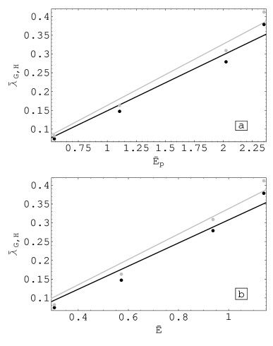
Figure 14: Lyapunov histories $\bar{\lambda}_{\text{G}}\left(t\right)$ (black dots) and $\bar{\lambda}_{\text{H}}\left(t\right)$ (grey dots), extrapolated to infinite evolution times, as a function of $\bar{E}_{\text{p}}$ (panel a) and $\bar{E}$ (panel b). The straight lines are the best linear fits. (For $\delta=0.6$, 0.45, 0.3 and $0.2$, with $\bar{\kappa}=1$ and $N=10$.)

Finally, our long-time analysis allows us to clarify what happens to the two scaling laws (44) and (45) on the approach to total equilibrium in the $t\rightarrow\infty$ limit where the Lyapunov histories saturate. In fact, a rather reliable extrapolation to this limit (in particular for larger energies) can be achieved by taking advantage of empirical evidence for the asymptotic evolution-time dependence $\sim\bar{t}^{-1/2}$ with which the Lyapunov histories approach the MLEs mue96 . (This finite evolution-time behavior is analogous to the finite-size behavior $\sim\left(Na\right)^{-1/2}$ mue96 ; ful01 which results from sampling ergodic states bol00 . On similar grounds, the width of Gaussian fluctuations around the mean value of the average Lyapunov exponent was argued to decay as $\bar{t}^{-1/2}$ bol00 .) Hence the new functions $\bar{\lambda}_{\text{G,H}}\left(\bar{t}^{-1/2}\right)$ can approximately be fitted by straight lines (with a potential systematic bias) and the MLEs determined as the intersections with the $\bar{t}^{-1/2}=0$ axis mue96 . Extrapolating the curves in Figs. 10 and 11 in this way to infinite evolution time yields our best estimates for the MLEs which we plot in Fig. 14 as a function of $\bar{E}_{\text{p}}$ (upper panel) and $\bar{E}$ (lower panel). These figures show that both dependencies remain to good accuracy linear. The best linear fits (also shown in the figures) are

$$\bar{\lambda}_{\text{G}}\left(\bar{E}_{\text{p}}\right)\simeq 0.149\bar{E}_{\text{p}},\text{ \ \ \ \ \ }\bar{\lambda}_{\text{H}}\left(\bar{E}_{\text{p}}\right)\simeq 0.163\bar{E}_{\text{p}},$$ (49)

and

$$\bar{\lambda}_{\text{G}}\left(\bar{E}\right)\simeq 0.308\bar{E},\text{ \ \ \ \ \ }\bar{\lambda}_{\text{H}}\left(\bar{E}\right)\simeq 0.338\bar{E}.$$ (50)

Equations (49) show that to an accuracy of at least about 10% the scaling law (44) found before full equilibration, with the same coefficient as in pure YM theory, indeed remains intact asymptotically. (First indications for this behavior were observed in Ref. hei97 on the basis of a trajectory for $t\leq 12000a$.) Qualitatively, this is also reflected in Fig. 12 where the ratios $\bar{\lambda}_{\text{G,H}}\left(t\right)/\bar{E}_{\text{p}}\left(t\right)$ start at around $1/6$ and asymptotically return to it for very large $t$ (while in the meantime deviating by maximally (i.e. for the largest $\delta$) about 20%, mainly when most of the energy is exchanged between the gauge and Higgs fields).

The Eqs. (49) also explain the $\bar{E}$ dependence of the asymptotic Lyapunov histories exhibited by the fits (50). Indeed, after full equilibration at $t\rightarrow\infty$ with $\bar{E}_{\text{G}}=\bar{E}_{\text{p}}/2=\bar{E}_{\text{H}}=\bar{E}$ one expects from $\bar{\lambda}_{\text{G,H}}\left(\bar{E}_{\text{p}}\right)=\alpha_{\text{G,H}}\bar{E}_{\text{p}}\simeq\bar{E}_{\text{p}}/6$ that

$$\bar{\lambda}_{\text{G,H}}\left(\bar{E}\right)=2\alpha_{\text{G,H}}\bar{E}\simeq\frac{1}{3}\bar{E}$$ (51)

which is within errors identical to Eqs. (50). Hence in equilibrium the linear dependence of the MLEs on $\bar{E}_{\text{p}}$ implies a linear dependence on $\bar{E}$ with twice the slope (as realized to good accuracy in the fits (49) and (50)). This fact went probably unnoticed in Ref. hei97 which argued against linear scaling of the $\bar{\lambda}_{\text{G,H}}$ with $\bar{E}$ on the basis of field evolution trajectories over maximally several thousand lattice time units, i.e. likely too short to bring the system close enough to equilibrium. (In addition, our above observation supports the diagnosis of Ref. ful01 which attributes the logarithmic energy dependence found numerically for several SU$\left(2\right)$-YM MLEs after very long evolution times to finite-size artefacts of the monodromy-matrix method.) More generally, linear scaling of $\bar{\lambda}_{\text{G,H}}$ with $\bar{E}_{\text{p}}$ implies a linear dependence on $\bar{E}$ in any time window during which $\bar{E}_{\text{p}}\propto\bar{E}$. This condition seems to be satisfied only when the gauge and Higgs sectors do not exchange relevant amounts of energy, however, i.e. only in the preequilibration phase and after mutual equilibration is essentially achieved. Nevertheless, the slopes of the $\bar{E}$ dependence in these two time intervals are different (5/9 and 1/3, respectively).

The above evidence for the linear dependence (44) of the MLEs on the average magnetic energy $\bar{E}_{\text{p}}$ to prevail for $t\rightarrow\infty$ appears consistent with our previous indications for the maximally chaotic mode to reside mainly in the gauge sector, with our finding that the scaling behavior (44) sets in way before the gauge fields have full access to the energy stored in the Higgs sector, and with the result that the ratios $\bar{\lambda}_{\text{G,H}}\left(t\right)/\bar{E}_{\text{p}}\left(t\right)$ saturate significantly faster than the $\bar{\lambda}_{\text{G,H}}\left(t\right)$ themselves.

IV.4 Maximal Lyapunov exponents of initially homogeneous magnetic fields

In this section we digress from our main subject and apply some of the numerical techniques developed above to the time evolution of spacially constant, non-Abelian magnetic fields. In the pioneering days of QCD such homogeneous magnetic fields were perturbatively established to be unstable in pure YM theory sav77 . This so-called Savvidy instability was later explored in the nonperturbative domain by numerical methods similar to ours tra92 ; mul92 . It provided early indications for the complexity of the Yang-Mills vacuum and has triggered the development of stochastic and chaotic concepts for vacuum structure and quark confinement bir294 ; far05 ; chaoconf . In the following we are going to study the impact of the matter (i.e. Higgs) fields on the Savvidy instability.

As a benchmark for comparison with the YMH case, we first reproduce the nonperturbative time evolution of the distance (29) between initially adjacent, homogeneous magnetic fields in pure YM theory on an $N=10$ lattice. The non-Abelian magnetic field is defined as $B_{\text{p}}=\arccos tr\left(U_{\text{p}}\right)$, and the fields are initialized with total energy $\bar{E}=0.57$ by setting $E_{x,i}^{a}\left(0\right)=0$, $B_{x,12}\left(0\right)=0.899,$ $B_{x,13}\left(0\right)=0.791$ and $B_{x,23}\left(0\right)=1.453$ for all $x$. In Fig. 15 we compare their logarithmic distance evolution to that of an initially randomized gauge field (cf. Sec. III.1) with the same energy. The constant magnetic field pair turns out to have about twice the average slope of $\ln d_{\text{G}}\left(t\right)$ in the linear region, i.e. the homogeneous magnetic field is substantially less stable than the random field. This result corroborates similar findings in Ref. mul92 .

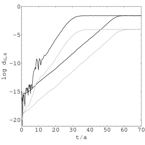
Figure 16: Evolution of the logarithmic distances (29) (black lines) and (30) (grey lines) for two initially neighboring, homogeneous, non-Abelian magnetic fields (ragged curves with larger slopes in the linear region) and for two initially neighboring random gauge-field configurations in YMH theory (with $\delta=0.3$, $\bar{R}=0.2$, $\bar{\kappa}=1$, $N=10$, $\bar{E}=0.572023$).

We now turn to the analogous time evolution of initially constant magnetic fields in YMH theory, again on a lattice with $N=10$ sites per dimension. As in all previous sections, the Higgs field is initialized at the spacially constant value $\bar{R}_{x}\left(0\right)=\bar{R}=0.2$, and the initial values $\dot{\phi}\left(0\right)=0$, $E_{x,i}^{a}\left(0\right)=0$ are imposed in order to satisfy Gauss’ law (27). The $B$ field is initialized at the values $B_{x,12}\left(0\right)=2.319,$ $B_{x,13}\left(0\right)=2.152$ and $B_{x,23}\left(0\right)=1.428$ for all $x$. We further choose $\delta=0.3$ and $\bar{\kappa}=1$ in order to inject the same total energy $\bar{E}=0.57$ as in the YM case above. The logarithmic distance evolution under these conditions is displayed in Fig. 16 for the gauge and Higgs field metrics (29) and (30), again together with its counterpart for a corresponding random field. As in the YM case, the homogeneous magnetic field produces about twice the slope in the linear region. Hence the presence of the matter fields seems neither to dampen nor to enhance the increased instability of the homogeneous magnetic field configurations relative to a random configuration of the same total energy. This seems to be consistent with our above evidence for the chaoticity of YMH theory to be dominated by the gauge sector.

The slopes of $\ln d_{\text{G}}\left(t\right)$ for both constant magnetic and random fields, however, are (in the linear region) about twice as large in the YMH example of Fig. 16 than in YM theory (Fig. 15). Probably this result depends rather strongly on the initial conditions, and especially on how they distribute the initial energy over the gauge and Higgs field sectors. Our above initial conditions were chosen to provide a demonstrative example for the presence of matter fields to strongly enhance the Savvidy instability. This massive impact raises the possibility that simulation results for those gauge-field instabilities which drive isotropization and thermalization in the aftermath of high-energy nuclear collisions could be significantly modified in the presence of quark fields as well (although they have smaller occupation numbers).

V Related equilibration processes in cosmology and nuclear collisions

In the following section we are going to discuss several aspects of nonequilibrium processes in the early Universe and in the aftermath of high-energy nuclear collisions which are pertinent in our context. We comment on the impact of the chaotic thermalization properties calculated above and on results of classical gauge-theory simulations related to ours. We also suggest a few promising extensions of our work which would help to clarify the role of chaotic thermalization processes after nuclear collisions and the nature of the “apparent” or “pre-” equilibrium at the beginning of the subsequent hydrodynamic evolution phase.

V.1 Early Universe

According to the inflation paradigm, the vacuum energy of one or more classical, scalar inflaton fields dominated the very early Universe. This energy caused a typically exponentially accelerated expansion period which very efficiently diluted particles and fluctuations inf . It left the universe in a supercooled, highly nonthermal state which was practically devoid of matter, radiation and entropy. Hundreds of models for the phenomenologically very successful inflationary scenario were proposed bas06 . A compelling “microscopic” theory, however, which is able to explain e.g. the nature of the inflaton(s) and the very specific properties of their dynamics, has not yet been established, partly because it involves unknown physics beyond the standard model.

For the post-inflationary reheating period, during which the Universe thermalized at a still very large “reheating temperature”, the theoretical situation is similar: there exist many scenarios and model calculations for specific processes whereas the underlying dynamics as a whole is not yet settled. During reheating a huge amount of entropy was released. All the matter and radiation of the present Universe was created and the energy density of the inflaton(s) was transformed into a hot and ultrarelativistic plasma. (Afterwards the Universe expanded essentially in the Friedman-Robertson-Walker geometry and cooled almost isoentropically according to the “hot-big-bang” scenario.) In the following we will be particularly interested in the (semi-) classical phases during the reheating period, when the large occupation numbers of the participating field modes made contributions from chaotic thermalization relevant.

The probably most important of these phases, referred to as preheating, is suggested to have taken place immediately after inflation kof94 . During this very short period, which lasted about $10^{-35}$ secs., particle production became explosive. Preheating can be induced either by a tachyonic instability of the inhomogeneous modes which accompany electroweak symmetry breaking fel01 , or by the stimulated decay of an almost homogeneous inflaton which coherently oscillates with an initial amplitude of the order of the Planck mass. In the latter case, the accelerated decay is the consequence of a parametric resonance with condensates composed of the produced particles kof94 . A detailed understanding of the preheating process is particularly crucial because the bulk of the initial conditions for the subsequent thermal history of the Universe are settled at its end. Since the homogeneous energy density of the inflaton transfers exponentially rapidly into highly occupied, inhomogeneous out-of-equilibrium modes, furthermore, the violently nonperturbative and nonequilibrium processes underlying preheating are amenable to classical lattice simulations mic04 .

After preheating, a variety of crucial thermalization processes began to drive the Universe towards equilibrium. Classical lattice simulations of such processes indicate, furthermore, that the infrared modes excited during preheating evolve towards a saturated occupation number distribution long before thermalization completes pod06 . Such effects have been interpreted as signs of “prethermalization”, characterized by an energy-pressure relation approximating an equation of state ber04 ; pod06 . Later on, the distributions move towards complete saturation by cascading towards ultraviolet and infrared modes (as in Kolmogorov wave turbulence). During the last and longest stage of equilibration, finally, the particle distributions become fully thermal . Simultaneously, the occupation numbers drop until quantum physics eventually dominates and classical simulations become ineffective.

Among the many important nonequilibrium processes which shape the reheating period are backreactions on the inflaton field which eventually stop particle production, violent and still nonperturbative particle rescattering events which very efficiently generate entropy, the nonthermal production of heavy particles as well as phase transitions. Further reheating processes which left crucial imprints in our present Universe are primordial magnetic field generation dia08 , topological and large-scale structure formation as well as baryogenesis pro97 , which created the observed abundance of baryons over antibaryons. In our context, baryogenesis is particularly interesting since it can efficiently proceed only far from equilibrium. As already mentioned, lattice simulations of classical real-time field evolution are a method of choice for the analysis of such processes. In fact, they turned out to be particularly useful for shedding light on the preheating phase whose immense particle production rate and condensate formation require a fully nonperturbative treatment while the generated, large (boson) occupation numbers ensure a classical field evolution preh .

In the following, we will focus on classical lattice simulations of cosmological pre- and reheating processes which were based on dynamics including the gauge-scalar sector of the standard model , i.e. the SU$\left(2\right)$ YMH theory with a fundamental Higgs doublet (1) . This theory has been used, notably, to explore the electroweak symmetry breaking transition esb . It underlies our own work, furthermore, and thus allows for some partial and qualitative comparisons – although the initial conditions (and the additional field content including e.g. an inflaton) required to describe cosmological situations differ considerably from the random ones which we have adopted above.

The analysis of electroweak baryogenesis at energies of the order of 100 GeV is, as already alluded to, an especially interesting application of the YMH model (1) and its extensions kuz85 ; pro97 . Such studies are mainly motivated by the question whether “minimal extensions” of the electroweak standard model, which implement e.g. additional neutral scalar inflaton field(s) or $CP$ violating couplings, are able to explain the observed baryon asymmetry of the present Universe. As a step towards clarifying this issue, the baryon (and lepton) number and $CP$ violating sphaleron transition rate and the Chern-Simons number diffusion in the unbroken phase were studied in Refs. amb91 ; tan96 ; amb97 ; moo99 . In a hybrid inflation scenario gar99 , based on an additional singlet inflaton which couples to the Higgs field to accelerate particle production (compared to only gravitational coupling), the nonequilibrium preheating dynamics was found to generate Chern-Simons number, a prerequisite for electroweak baryogenesis, locally and stochastically gar04 . (For some cautionary remarks on the reliability of classical lattice results in this preheating scenario for baryogenesis see Ref. moo01 .) In the same dynamical framework, primordial magnetic fields are produced with sufficient magnitude and correlations to act as seeds for the magnetic fields observed in galaxies and galaxy clusters today dia08 . Electroweak baryogenesis during a cold electroweak transition with tachyonic preheating (induced by a spinodal Higgs field instability) and additional $CP$ violation generated by a coupling of the Higgs field to the topological charge density of the gauge field, has been investigated in Ref. tra03 . The particle distribution functions of the Higgs and gauge fields (on which kinetic theory is based) were extracted in Ref. sku03 from the correlators of the simulated classical fields, with the electroweak phase transition modeled by a quench.

Our main goal in the present paper was to study generic chaotic thermalization properties of YMH theory on the basis of random initial conditions. In this respect, our work differs from the more specialized simulations discussed above (which partly also include additional dynamics). Although this prevents a quantitative comparison of the results, we believe that the chaotic thermalization processes which we have analyzed should be relevant for most of the mentioned post-inflationary pre- and reheating processes as well. By adapting the initial conditions to cosmological situations, in particular, one could directly investigate the contributions of deterministic chaos, as measured by the Lyapunov exponents, to specific nonequilibrium processes. It would for example be interesting to follow the sphaleron transition and magnetic field production rates during the different stages of chaotic thermalization. It would also be useful to study the impact of the lattice spacing on the chaotic thermalization rates moo01 and to include physics beyond the standard model, e.g. an inflaton field, into the analysis.

V.2 Nuclear collisions

Thermalization properties of excited quark-gluon matter, as produced at the SPS, RHIC, LHC and (future) FAIR colliders, have been intensely studied in various approaches of increasing sophistication (see Refs. mro206 for recent reviews). The detailed local equilibration mechanisms are of central importance for the heavy-ion programs since they determine whether a new, deconfined state of matter – the quark-gluon plasma – can be locally thermalized in the aftermath of high-energy nuclear collisions, i.e. whether the produced system equilibrates fast enough for thermodynamic concepts to apply before it disintegrates.

The thermalization issue became even more intriguing when RHIC results showed that the produced matter starts to behave collectively after times of less than $1$ fm/$c$ and is subsequently described by essentially ideal Bjorken hydrodynamics with almost maximal elliptic flow rhic . These findings are generally interpreted as a surprisingly fast apparent thermalization of the system, which minimally requires the isotropization of the long-wavelength modes participating in the hydrodynamic behavior arn205 and perhaps the onset of prethermalization ber04 . In any case, the very short (pre-) equilibration time cannot be explained by weakly coupled parton-parton collisions alone mro206 ; arn03 .

The time evolution of a typical RHIC reaction (which is sometimes referred to as a “little bang” to emphasize similarities with the big bang of the Universe) begins with very hard initial interactions between the high-momentum partons of the colliding nuclei. These generate the highest-momentum particles in the final state. Afterwards, at about $t\sim 0.2$ fm/$c$, most of the soft particles in the final state are coherently produced and form a nonequilibrium system (sometimes called a “glasma” lap06 ) of high energy density. The “bottom-up” thermalization scenario bai01 assumes that the initial properties of this system are determined by the QCD saturation mechanism , i.e. that they are dominated by coherent small-$x$ gluons of a very high density. These gluons originate from the low-$x$ part of the nuclear wavefunctions ($x=p_{\text{t}}/\sqrt{s}$ where $s$ is the total energy) and carry transverse momenta $p_{\text{t}}$ of the order of the saturation scale $Q_{\text{s}}$. Since for RHIC collisions $Q_{\text{s}}\sim 1$ GeV $\gg\Lambda_{\text{QCD}}$, this initial state should be amenable to weak-coupling techniques . In the color glass condensate (CGC) model ian03 , for example, the highly populated small-$x$ gluon states are treated as the soft modes of classical Yang-Mills fields with typically large amplitudes while the hard field modes are represented by static sources.

More generally, as long as the gluon mode occupation numbers stay large enough to suppress quantum effects, their evolution can be described in terms of classical gauge fields which may be simulated fully nonperturbatively on a spacial lattice. Over the last years, an increasing amount of such numerical simulations was performed for the gauge groups SU$\left(2\right)$ and SU$\left(3\right)$ in one, two and three spacial dimensions. The dynamical settings included the CGC model kra99 ; rom06 , hot-thermal-loop (HTL) effective theories (equivalent to a collisionless Vlasov equation) arn03 ; htl ; arn05 and equations of Wong-Yang-Mills type dum05 ; dum07 ; bod07 , subject to minijet or bottom-up initial conditions. Among the calculated observables were e.g. energy densities and gluon multiplicity distributions.

Numerical simulations confirmed, in particular, that sufficiently anisotropic parton momentum distributions, as typically produced in heavy-ion collisions, can induce the onset of a very fast, collective isotropization and (pre-) thermalization driven by non-Abelian filamentation instabilities dum05 . These Weibel-type plasma instabilities generate an initially exponential growth of the soft-mode occupation numbers even at relatively weak couplings mro06 ; mro206 ; plinst . The expansion of the system can strongly reduce this growth, however, and the non-Abelian self-interactions appear to rapidly limit it (in three spacial dimensions) to at most linear growth arn05 . This happens when the (magnetic) energy deposited in the soft fields returns sufficiently fast to the hard fields, either by plasmon excitation effects similar to Kolmogorov wave turbulence arn05 ; ber08 or via a rapid avalanche dum07 . Applications of the CGC and HTL effective theories are limited to the weak-coupling and small-amplitude regimes, however, which ensure a sufficient scale separation between the hard parton and soft gauge-field momenta . This technical limitation can be avoided by describing the whole system as a classical statistical Yang-Mills ensemble with an UV lattice cutoff to substitute for the quantum mechanical suppression of thermal short-distance effects. Hard and soft modes are thus originating from the same gauge field and treated on the same footing, which allows for nonperturbatively large amplitudes.

The numerical simulations described in the present paper are based on the same interpretation of the classical lattice fields. Although we focused on the thermalization of gauge-Higgs matter by chaotic instabilities, which at first seems to be a rather different mechanism, there are several commonalities with equilibration via mean-field plasma instabilities. In fact, both are collective processes which shape the momentum distribution of the classical gauge fields, and both lead to substantially faster gluon equilibration rates than collisional thermalization. This becomes explicit in relaxation times $\tau\sim\lambda^{-1}\sim 0.5$ fm/$c$ at typical RHIC energies. (The chaotic relaxation time tends to become even smaller for SU$\left(3\right)$ gauge fields gon93 ). As pointed out in Ref. bol00 , incidentally, relaxation times of this order imply that fluctuations around the mean transverse momentum produced in nuclear collisions are very small (of order $10^{-2}$, i.e. at the percent level, for typical reaction volumes (5 fm)³ and times (0.5 fm) at RHIC), as indeed observed in event-by-event fluctuations.

On the other hand, there are remarkable differences between chaotic and plasma instabilities. The maximally chaotic modes are very efficient in generating entropy directly, for instance, while the filament instabilities lead to a reversible isotropization (at the mean-field level) which just creates more efficient conditions for the subsequent entropy production. Hence Weibel-type plasma instabilities per se seem hardly to affect the MLE values, although they could indirectly contribute to our chaotic thermalization if the random initial conditions generate a sufficiently anisotropic momentum distribution of the gauge fields. It is tempting to speculate, then, that even under RHIC initial conditions the maximally chaotic modes may lead to faster thermalization than plasma instabilities because they generate entropy in a probably more efficient one-step process. Moreover, the maximal chaotic instabilities select at any time the most unstable direction in phase space and thus remain optimally fast during the entire (classical) thermalization process, whereas the filament instabilities are damped by the gauge field’s non-Abelian self-interactions .

As mentioned above, a long-term perspective of our work is to understand the role of chaotic thermalization mechanisms during the classical evolution phases in the aftermath of nuclear collisions. The focus of the present paper was more limited and preparatory, however, namely to map out generic chaotic thermalization properties of non-Abelian gauge systems in the presence of scalar matter. (Classical Higgs fields were included because of their role in the early Universe and because they can be treated on the same footing as the gauge fields. Quarks, on the other hand, would have to be implemented either as particles or as solutions of the Dirac equation in the background of the classical fields, as e.g. in soliton models for baryons lee77 .) For this reason, we have chosen random initial conditions instead of the more specialized ones required to describe the physical situation after a nuclear collision (or during the reheating phase of the early Universe). Our program could naturally be extended by adapting it to those initial conditions with a strongly anisotropic momentum distribution which characterize the hot system created by a high-energy nuclear collision. The chaotic properties of plasma-instability-, collision- and cascade-driven thermalization processes could then be quantified in terms of the corresponding maximal Lyapunov exponents, thereby relating the chaotic thermalization and entropy production rates to the time scales of more conventional equilibration processes. (The large difference between the Lyapunov exponents of randomly and coherently initialized fields (cf. Secs. IV.1 and IV.4) show that they can depend strongly on the initial conditions.)

In addition, one may extract a more detailed picture of the chaotic equilibration processes by following e.g. the evolution of the field modes’ momentum distributions and their anisotropy, as well as the evolution of pressure, entropy etc. simultaneously with the Lyapunov histories. For specific comparisons with the effective CGC and HTL dynamics, it would also be interesting to follow the growth rate of the gauge field’s Fourier coefficients. This would further clarify how far chaotic evolution is consistent with the bottom-up thermalization scenario, according to which the copiously produced soft gluons (which initially carry only a small fraction of the total energy) draw energy from the hard gluons and thermalize very efficiently. The decay of the remaining hard gluons then reheats the soft gluonic background until it enters the hydrodynamic evolution stage. In fact, in reductions of the Yang-Mills dynamics to a few degrees of freedom, chaotic thermalization was found to start (under suitable initial conditions) among the softer modes as well bir295 . Moreover, the chaotic behavior of the soft modes turns out to be driven by the soft-hard mode coupling, which provides an efficient mechanism for energy transfer from high frequency modes to a low-energy multiparticle final state. (Related findings for the scattering of two classical SU$\left(2\right)$ YM and YMH wave packets were reported in Ref. hu95 .)

VI Summary and conclusions

We have investigated chaotic instability and thermalization properties of classical gauge and matter fields in the unbroken phase of SU$\left(2\right)$ Yang-Mills-Higgs theory on a spacial lattice. Since equilibration proceeds mainly through the most unstable field modes, we have focused on a quantitative survey of the most chaotic time evolution patterns in terms of maximal Lyapunov exponents (which measure the logarithmic distance growth rates between initially neighboring gauge and Higgs fields).

A main goal of our investigation was to explore the impact of the fundamental doublet of scalar matter fields on the chaotic behavior of the gauge dynamics. Towards this end, we first confirmed and extended previous evidence for the Yang-Mills-Higgs system to equilibrate over two drastically different time scales: individually, the rather weakly coupled gauge and Higgs sectors reach a preequilibrium phase after only a few lattice time units, whereas their mutual equilibration is substantially delayed by the matter fields and takes far longer than $10^{4}$ units to complete. Accordingly, we have generated two sets of maximal Lyapunov exponents for initially random fields: a larger one extracted from the field separation rates at the preequilibration stage, and a smaller one obtained from long-time trajectories extrapolated to infinite evolution time and thus to full equilibrium.

The first set was designed to cover a representative part of the weakly coupled phase space and contains about 80 Lyapunov exponents. In view of its non-negligible finite-time errors, this set was mainly used to study general characteristics of the exponents including their energy, coupling-parameter and lattice-size dependence. We found the signs of the whole set to be positive (in contrast to results in the broken phase), which implies that chaos is at least approximately universal in the symmetric phase. (Possible exceptions may include small nonergodic niches as previously encountered in the Yang-Mills phase space.) Yang-Mills-Higgs theories with gauge groups containing SU$\left(2\right)$ as a subgroup are therefore chaotic as well. In the energy and coupling ranges where both finite-size and lattice-spacing errors should be under control, our Lyapunov exponents on lattices with between $10^{3}$ and $30^{3}$ sites were indeed found to be within statistical uncertainties identical. In addition, we found the maximal Lyapunov exponents extracted during the preequilibrium phase to be almost independent of the Higgs self-coupling. This indicates that the nonlinear interactions in the Higgs sector provide a relatively minor contribution to the chaoticity of the system.

In order to survey the important and previously unexplored asymptotic regions of the Yang-Mills-Higgs phase space, we have additionally followed several field evolution trajectories over the exceptionally long periods required to approach total equilibrium. In particular, we have investigated the long-time behavior of eight Lyapunov histories, i.e. logarithmic separation rates between initially neighboring fields, over 20000 lattice units. After extrapolation to infinite evolution times they provide our best estimates for the maximal Lyapunov exponents. All Lyapunov histories turn out to decrease monotonically with time and saturate relatively slowly even after the energy has attained almost complete equipartition. At larger values of the Higgs self-coupling the Lyapunov histories vary less strongly during time evolution while their saturation is further delayed. Moreover, the Lyapunov histories divided by the average plaquette energy saturate faster than the Lyapunov histories themselves. This foreshadows an early onset of their linear scaling relation in the equilibrated system (see below). The long-time behavior of the Lyapunov histories provides reliable estimates for the finite-time errors of the Lyapunov exponents, furthermore, and quantifies in particular how much they are overestimated in the preequilibrium phase.

The physical interest in Lyapunov exponents of gauge fields originates partly from evidence for their linear relation to the plasmon damping rates at weak coupling. This relation relies on the empirically identified linear dependence of the maximal Lyapunov exponents on the average magnetic gauge-field energy. We have therefore systematically scrutinized the accuracy and validity range of this scaling relation on the basis of our full data set. Both during the rather long preequilibrium period, i.e. before gauge and Higgs sectors have exchanged substantial amounts of energy, and after full thermalization we have indeed found the Lyapunov histories to scale within errors linearly with the average gauge-field energy. More specifically, both during preequilibrium and after complete equilibration our results establish the relation $\bar{\lambda}_{\text{G,H}}\simeq\bar{E}_{\text{p}}/6$ between the maximal Lyapunov exponents and the average plaquette energy. This relation was previously encountered in pure Yang-Mills theory and seems to be a rather exclusive property of non-Abelian gauge theories. It implies that the Lyapunov exponents for any given gauge field energy, extracted either from the gauge or Higgs field separation rates, remain within errors independent of the presence of the Higgs field. This lends additional credence to the suggested equality between the Lyapunov exponents and twice the static plasmon damping rates of quantum Yang-Mills-Higgs theory at high temperatures and weak coupling. In addition, we have established that both during the preequilibrium stage and after full thermalization the maximal Lyapunov exponents also scale linearly with the total energy. This is in contrast to previous expectations and turns out to be a consequence of the proportionality between gauge and total energy during both phases.

We have furthermore studied how interactions with the Higgs field affect the Savvidy instability of constant non-Abelian magnetic fields. As a benchmark, we have first obtained the maximal Lyapunov exponent for an initially constant magnetic field in pure Yang-Mills theory and found it about twice as large as that of a randomly initialized field under otherwise equal conditions. We have then computed the analogous Lyapunov exponent in Yang-Mills-Higgs theory for initially homogeneous magnetic and Higgs fields at the same total energy and found it still to be about 2 times larger than for randomized fields. Hence the additional matter fields seem neither to dampen nor to enhance the Savvidy instability relative to that of random fields of the same energy. Depending on the initial energy distribution between gauge and Higgs fields, however, the presence of matter fields can have a strong impact on the absolute magnitude of the magnetic field’s instability. In order to demonstrate this, we have provided an example in which the matter fields approximately double the maximal Lyapunov exponent of the gauge field.

In all simulations described above, we found the Lyapunov histories to be within errors of at most a few percent independent of the underlying distance measure and of whether they were obtained in the gauge or Higgs field’s phase space. This independence turns out to hold both during the preequilibration phase and towards full equilibrium, and both for initially homogeneous and random fields. Hence it confirms the general expectation that the divergence rates of the most unstable modes should be equally measurable by any reasonable metric in field space. The behavior of the Lyapunov histories depends somewhat on the stage of the thermalization process, however. Before gauge and Higgs fields have exchanged substantial amounts of energy, the divergence rate in the gauge sector turns out to be slightly larger than in the Higgs sector, while it becomes marginally smaller during later phases of equilibration. A previous estimate of an about 15% smaller logarithmic Higgs field separation rate, based on a single trajectory, was therefore probably contaminated by numerical uncertainties.

Our above results strengthen the evidence for the gauge dynamics to provide the main source of chaotic instability in the Yang-Mills-Higgs system. The matter fields, in contrast, seem to play a subordinate role (similar to the quark fields shortly after a nuclear collision). The evidence includes the fast preequilibration of the gauge sector, the observation that the Higgs sector seems to have little impact on the ratio between the constant magnetic and random field Lyapunov exponents, the linear dependence of the maximal Lyapunov exponents on the average gauge-field energy alone, the finding that this scaling behavior sets in way before the gauge fields have full access to the energy stored in the Higgs sector, and in particular the fact that the values of the maximal Lyapunov exponents for a given plaquette energy turn out to be within errors identical to those in pure Yang-Mills theory. Moreover, the nonlinear Higgs dynamics seems not to contribute substantially to the maximally unstable mode, at least not in the range of relatively weak couplings where lattice artefacts are under control. Indeed, at the preequilibration stage the Lyapunov histories turn out to be practically independent of the Higgs self-coupling, and even afterwards the coupling dependence remains moderate.

Nevertheless, we found the scalar matter fields to have a major impact on the thermalization of the gauge system. As we have shown, their presence can strongly enhance the absolute divergence rate between neighboring gauge fields, both homogeneous and random. Moreover, the maximally chaotic mode has an almost immediate effect on the Higgs sector, as witnessed by the fact that its separation rate can be monitored equally well by following the distance evolution between neighboring Higgs fields. Finally, the presence of the Higgs fields massively prolongs the equilibration of the system as a whole, at least at weak coupling. This qualitative effect may be robust enough to prevail in the case of fermionic matter, and hence be relevant for understanding the equilibration properties of the highly excited quark-gluon matter produced in ultrarelativistic nuclear collisions.

Figure 1: The average energy per plaquette $\bar{E}_{\text{p}}$ as a function of the initialization parameter $\delta$.

Figure 2: Time evolution of the energy (per degree of freedom) stored in the gauge field $E_{\text{G}}$ (uppermost initially horizontal line) and in the Higgs field $E_{\text{H}}$ (lowermost initially horizontal line) and their sum, i.e. the (conserved) total energy $E$ (horizontal line). The initially oscillating line starting at zero is the electric gauge-field energy $E_{\text{el}}$, the one starting at the total initial gauge-field energy is the magnetic (potential) gauge field energy $E_{\text{mag}}$. (The initial conditions for the underlying trajectory were $\delta=0.2$, $\bar{R}=0.2$, $\bar{\kappa}=$ $1$, $N=10$ and $\Delta t=10^{-4}$.)

Figure 3: Same as in Fig. 2, but for the trajectory subject to the initial conditions $\delta=1$, $\bar{R}=0.2$, $\bar{\kappa}=$ $1$ and $N=10$.

Figure 15: Logarithmic distance evolution for initially neighboring, homogeneous, non-Abelian magnetic fields (ragged curve) and for initially neighboring randomized gauge-field configurations (smooth curve) in YM theory (with $N=10$ and $\bar{E}=0.572023$).

- (1) U. Heinz, arXiv:hep-ph/0407360; P. Jacobs and X.-N. Wang, Prog. Part. Nucl. Phys. 54, 443 (2005).
- (2) B.A. Bassett, S. Tsujikawa and D. Wands, Rev. Mod. Phys. 78, 537 (2006).
- (3) A.D. Linde, Phys. Lett. B 96, 289 (1980).
- (4) A.V. Selikhov and M. Gyulassy, Phys. Lett. B 316, 373 (1993).
- (5) E. Braaten and R.D. Pisarski, Phys. Rev. D 42, 2156 (1990).
- (6) R.D. Pisarski, arXiv:0810.4585.
- (7) B. Müller and A. Trayanov, Phys. Rev. Lett. 68, 3387 (1992).
- (8) T.S. Biró, S.G. Matinyan, and B. Müller, Chaos and Gauge Field Theory, World Scientific, Singapore, 1994; T.S. Biró, Á. Fülöp, C. Gong, S.G. Matinyan, B. Müller and A. Trayanov, Lecture Notes in Physics 494, 164 (1997).
- (9) T. S. Biró, C. Gong and B. Müller, Phys. Rev. D 52, 1260 (1995).
- (10) J.P. Blaizot and E. Iancu, Phys. Rep. 359, 355 (2002).
- (11) Proceedings of the Workshop on Strong and Electroweak Matter, Eger, Hungary, 1997, edited by F. Csikor and Z. Fodor (World Scientific, Singapore, 1998); M. Dine and A. Kusenko, Rev. Mod. Phys. 76, 1 (2003).
- (12) M.B. Hindmarsh and T.W.B. Kibble, Rept. Prog. Phys. 58, 477 (1995); I. Tkachev, S. Khlebnikov, L. Kofman and A.D. Linde, Phys. Lett. B 440, 262 (1998).
- (13) N. Armesto et al., J. Phys. G 35, 054001 (2008).
- (14) S. Mrówczyński, Phys. Lett. B 393, 26 (1997); Acta Phys. Pol. B 39, 1665 (2008).
- (15) J. Ambjorn, T. Askgaard, H. Porter and M.E. Shaposhnikov, Nucl. Phys. B 353, 346 (1991).
- (16) H. Forkel, Phys. Rev. D 73, 105002 (2006); Int. J. Mod. Phys. E 16, 2789 (2007).
- (17) R. Fariello, H. Forkel and G. Krein, Phys. Rev. D 72, 105015 (2005); H. Forkel, arXiv:0810.2098, Int. J. Mod. Phys. D, to appear.
- (18) J. Kogut and L. Susskind, Phys. Rev. D 11, 395 (1975).
- (19) S.A. Chin, O.S. van Roosmalen, E.A. Umland and S.E. Koonin, Phys. Rev. D 31, 3201 (1985).
- (20) T.S. Biró, C. Gong, B. Müller and A. Trayanov, Int. J. Mod. Phys. C 5, 113 (1994).
- (21) G. Benettin, L. Galgani, A. Giorgilli and J.-M. Strelcyn, Meccanica 15, 21 (1980); M. D. Hartl, Phys. Rev. D 67, 024005 (2003).
- (22) C. Gong, Phys. Rev. D 49, 2642 (1994). For more recent simulations on somewhat larger lattices see Ref. bol00 for the real Lyapunov spectrum and Ref. ful01 for the complex Lyapunov spectrum (and the Kolmogorov-Sinai entropy) from the eigenvalues of the monodromy matrix.
- (23) J. Bolte, B. Müller and A. Schäfer, Phys. Rev. D 61, 054506 (2000).
- (24) Á. Fülöp and T.S. Biró, Phys. Rev. C 64, 064902 (2001)
- (25) B. Müller, Duke University Report No. DUKE-TH-96-118, chao-dyn/9607001 (unpublished).
- (26) U. Heinz, C.R. Hu, S. Leupold, S.G. Matinyan and B. Müller, Phys. Rev. D 55, 2464 (1997).
- (27) T. S. Biró and M.H. Thoma, Phys. Rev. D 54, 3465 (1996).
- (28) J. Ambjorn, T. Aksgaard, H. Porter and M.E. Shaposhnikov, Nucl. Phys. B 353, 346 (1991).
- (29) H.B. Nielsen, H.H. Rugh and S.E. Rugh, arXiv:chao-dyn/9605013; arXiv:hep-th/9611128.
- (30) J. Zakrzewski, Phys. Lett. B 327, 67 (1994).
- (31) P. Dahlqvist and G. Russberg, Phys. Rev. Lett. 65, 2837 (1990).
- (32) S.G. Matinyan, G.K. Savvidi and N.G. Ter-Arutyunyan-Savvidi, JETP Lett. 34, 590 (1981).
- (33) G.P. Berman, Yu.I. Man’kov and A.F. Sadreev, Sov. Phys. JETP 61, 415 (1985).
- (34) S.G. Matinyan and B. Müller, Phys. Rev. Lett. 78, 2515 (1997).
- (35) C. Gong, Phys. Lett. B 298, 257 (1993).
- (36) A. Krasnitz, Nucl. Phys. B 455, 320 (1995).
- (37) G. K. Savvidy, Phys. Lett. B 71, 133 (1977).
- (38) A. Trayanov and B. Müller, AIP Conference Proceedings 260, 280 (1992).
- (39) See e.g. H.B. Nielsen and P. Olesen, Nucl. Phys. B 160, 380 (1979); G.Z. Baseyan, S.G. Matinyan, and G.K. Savvidy, Sov. Phys. JETP 53, 247 (1979) [Zh. Eksp. Teor. Fiz. 29, 641 (1979)]; J. Ambjorn and P. Olesen, Nucl. Phys. B 170, 60 (1980); S.G. Matinyan, G.K. Savvidy, and N.G. Ter-Arutyunyan-Savvidy, ibid, 80, 830 (1981); Sov. Phys. JETP 53, 421 (1981) [Zh. Eksp. Teor. Fiz. 80, 830 (1981)]; P. Olesen, Nucl. Phys. B 200, 381 (1982); G.K. Savvidy, Nucl. Phys. B 246, 302 (1984); W.H. Steeb, J.A. Louw, and C.M. Villet, Phys. Rev. D 33, 1174 (1986); A. Giansanti and P.D. Simic, Phys. Rev. D 38, 1352 (1988); T. Biro, M. Feurstein and H. Markum, Heavy Ion Phys. 7, 235 (1998).
- (40) A.D. Linde, Particle Physics and Inflationary Cosmology, Harwood, Chur, Switzerland (1990); A.R. Liddle and D.H. Lyth, Cosmological inflation and large-scale structure, Cambridge University Press, Cambridge (2000); J. Gonzalo, Inflationary cosmology revisited, World Scientific, Singapore (2005); M. Lemoine, J. Martin and P. Peter (eds.), Inflationary Cosmology, Lect. Notes in Physics 0738, Springer, New York (2008).
- (41) L. Kofman, A.D. Linde and A.A. Starobinsky, Phys. Rev. Lett. 73, 3195 (1994); 76, 1011 (1996); Phys. Rev. D 56, 3258 (1997); Y. Shtanov, J.H. Traschen and R.H. Brandenberger, Phys. Rev. D 51, 5438 (1995); G.N. Felder, J. Garcia-Bellido, P.B. Greene, L. Kofman, A.D. Linde and I. Tkachev, Phys. Rev. Lett. 87, 011601 (2001).
- (42) G. Felder, J. García-Bellido, P. Greene, L. Kofman, A.D. Linde and I. Tkachev, Phys. Rev. Lett. 87, 011601 (2001); G. Felder, L. Kofman and A.D. Linde, Phys. Rev. D 64, 123517 (2001).
- (43) R. Micha and I.I. Tkachev, Phys. Rev. D 70, 043538 (2004).
- (44) D. Podolsky, G.N. Felder, L. Kofman and M. Peloso, Phys. Rev. D 73, 023501 (2006).
- (45) J. Berges, Sz. Borsány and C. Wetterich, Phys. Rev. Lett. 93, 142002 (2004).
- (46) A. Díaz-Gil, J. García-Bellido, M. García-Pérez and A. González-Arroyo, Phys. Rev. Lett. 100, 241301 (2008).
- (47) J. García-Bellido, M. García Pérez and A. González-Arroyo, Phys. Rev. D 69, 023504 (2004); A. Díaz-Gil, J. García-Bellido, M. García Pérez and A. González-Arroyo, Phys. Rev. Lett. 100, 241301 (2008); A. Rajantie, P.M. Saffin and E.J. Copeland, Phys. Rev. D 63, 123512 (2001); E.J. Copeland, D. Lyth, A. Rajantie and M. Trodden, Phys. Rev. D 64, 043506 (2001); A. Tranberg and J. Smit, JHEP 08, 012 (2006); A. Tranberg, J. Smit and M. Hindmarsh, JHEP 01, 034 (2007).
- (48) W.H. Tang and J. Smit, Nucl. Phys. B 510 (1998) 401; G.D. Moore and N. Turok, Phys. Rev. D 55 (1997) 6538; G.D. Moore and K. Rummukainen, Phys. Rev. D 63 (2001) 045002; M. Hindmarsh and A. Rajantie, Phys. Rev. D 64 (2001) 065016.
- (49) V.A. Kuzmin, V.A. Rubakov and M.E. Shaposhnikov, Phys. Lett. B 155, 36 (1985).
- (50) W.H. Tang and J. Smit, Nucl. Phys. B 482, 265 (1996).
- (51) J. Ambjørn and A. Krasnitz, Nucl. Phys. B 506, 387 (1997); G.D. Moore and N. Turok, Phys. Rev. D 56, 6533 (1997).
- (52) G.D. Moore, Phys. Rev. D 59, 014503 (1998); D. Bödeker, G.D. Moore and K. Rummukainen, Phys. Rev. D 61, 056003 (2000); B.-J. Nauta and A. Arrizabalaga, Nucl. Phys. B 635, 255 (2002).
- (53) J. Garcia-Bellido, D.Y. Grigoriev, A. Kusenko and M.E. Shaposhnikov, Phys. Rev. D 60, 123504 (1999).
- (54) J. Garcia-Bellido, M. Garcia Perez and A. Gonzalez-Arroyo, Phys. Rev. D 69, 023504 (2004).
- (55) G.D. Moore, JHEP 11, 021 (2001).
- (56) A. Tranberg and J. Smit, JHEP 11, 016 (2003).
- (57) J.-I. Skullerud, J. Smit and A. Tranberg, JHEP 08, 045 (2003).
- (58) X.-N. Wang, Phys. Rep. 280, 287 (1997); K. Geiger, Phys. Rep. 258, 237 (1995); B. Zhang, Comput. Phys. Commun. 104, 70 (1997).
- (59) E. Shuryak, Phys. Rev. Lett. 68, 3270 (1992).
- (60) P. Arnold, Int. J. Mod. Phys. E 16, 2555 (2007); S. Mrówczyński, PoS (CPOD2006) 042, (2006).
- (61) I. Arsene et al. (BRAHMS Collaboration), Nucl. Phys. A 757, 1 (2005); K. Adcox et al. (PHENIX Collaboration), Nucl. Phys. A 757, 184 (2005); B. B. Back et al. (PHOBOS Collaboration), Nucl. Phys. A 757, 28 (2005); J. Adams et al. (STAR Collaboration), Nucl. Phys. A 757, 102 (2005).
- (62) P. Arnold, J. Lenaghan, G.D. Moore and L.G. Yaffe, Phys. Rev. Lett. 94, 072302 (2005).
- (63) P. Arnold, J. Lenaghan and G.D. Moore, JHEP 08, 002 (2003).
- (64) T. Lappi and L. McLerran, Nucl. Phys. A 772, 200 (2006).
- (65) R. Baier, A.H. Mueller, D. Schiff and D.T. Son, Phys. Lett. B 502, 51 (2001); Phys. Lett. B 539, 46 (2002).
- (66) K. Kajantie, P.V. Landshoff and J. Lindfors, Phys. Rev. Lett. 59, 2527 (1987); K.J. Eskola, K. Kajantie and J. Lindfors, Nucl. Phys. B 323, 37 (1989); J.-P. Blaizot and A.H. Mueller, Nucl. Phys. B 289, 847 (1987).
- (67) E. Shuryak, J. Phys. G 30, S1221 (2004).
- (68) E. Iancu and R. Venugopalan, in Quark gluon plasma 3, ed. by R.C. Hwa and X.N. Wang, World Scientific, Singapore (2003).
- (69) A. Krasnitz and R. Venugopalan, Nucl. Phys. B 557, 237 (1999); Phys. Rev. Lett. 84, 4309 (2000); ibid. 86, 1717 (2001); ibid. 87, 192302 (2001).
- (70) P. Romantschke and R. Venugopalan, Phys. Rev. Lett. 96, 062302 (2006); Phys. Rev. D 74, 045011 (2006).
- (71) S. Mrówczyński, Phys. Lett. B 214, 587 (1988); S. Mrówczyński, A. Rebhan, and M. Strickland, Phys. Rev. D 70, 025004 (2004); P. Romatschke and A. Rebhan, Phys. Rev. Lett. 97, 252301 (2006); B. Schenke and M. Strickland, Phys. Rev. D 74, 065004 (2006); B. Schenke, M. Strickland, C. Greiner, and M. H. Thoma, Phys. Rev. D 73, 125004 (2006).
- (72) P. Romatschke and M. Strickland, Phys. Rev. D 68, 036004 (2003); 70, 116006 (2004); P. Arnold, G.D. Moore and L.G. Yaffe, Phys. Rev. D 72, 054003 (2005); A. Rebhan, P. Romantschke and M. Strickland, JHEP 09, 041 (2005); P. Arnold and G.D. Moore, Phys. Rev. D 73, 025006 (2006); 73, 025013 (2006).
- (73) A. Dumitru and Y. Nara, Phys. Lett. B 621, 89 (2005).
- (74) A. Dumitru, Y. Nara and M. Strickland, Phys. Rev. D 75, 025016 (2007).
- (75) D. Bödeker and K. Rummukainen, JHEP 07, 022 (2007).
- (76) A. Rebhan, P. Romatschke, and M. Strickland, Phys. Rev. Lett. 94, 102303 (2005); A. Rebhan, P. Romatschke and M. Strickland, JHEP 09, 041 (2005); P. Arnold and G.D. Moore, Phys. Rev. D 76, 045009 (2007); J. Berges, D. Gelfand, S. Scheffler and D. Sexty, Phys. Lett. B 677, 210 (2009).
- (77) J. Berges, S. Scheffler and D. Sexty, arXiv:0811.4293
- (78) R. Friedberg and T.D. Lee, Phys. Rev. D 15, 1694 (1977); Phys. Rev. D 16, 1096 (1977); L. Bayer, H. Forkel and W. Weise, Z. Phys. A 324, 365 (1986).
- (79) T.S. Biró, S.G. Matinyan and B. Müller, Phys. Lett. B 362, 29 (1995).
- (80) C.R. Hu, S.G. Matinyan, B. Müller, A. Trayanov, T.M. Gould, S.D.H. Hsu and E.R. Poppitz, Phys. Rev. D 52, 2402 (1995); C.R. Hu, S.G. Matinyan, B. Müller, Phys. Rev. D 54, 2175 (1996).