CARS: The CFHTLS-Archive-Research Survey
II. Weighing dark matter halos of Lyman-break galaxies at $z$=3-5

Abstract

Aims. We measure the clustering properties for a large samples of $u$- ($z\sim 3$), $g$- ($z\sim 4$), and $r$- ($z\sim 5$) dropouts from the Canada-France-Hawaii Telescope Legacy Survey (CFHTLS) Deep fields.

Methods. Photometric redshift distributions along with simulations allow us to de-project the angular correlation measurements and estimate physical quantities such as the correlation length, halo mass, galaxy bias, and halo occupation as a function of UV luminosity.

Results. For the first time we detect a significant one-halo term in the correlation function at $z\sim 5$. The comoving correlation lengths and halo masses of LBGs are found to decrease with decreasing rest-frame UV-luminosity. No significant redshift evolution is found in either quantity. The typical halo mass hosting an LBG is $M\ga 10^{12}h^{-1}M_{\odot}$ and the halos are typically occupied by less than one galaxy. Clustering segregation with UV luminosity is clearly observed in the dropout samples, however redshift evolution cannot clearly be disentangled from systematic uncertainties introduced by the redshift distributions. We study a range of possible redshift distributions to illustrate the effect of this choice. Spectroscopy of representative subsamples is required to make high-accuracy absolute measurements of high-$z$ halo masses.

1 Introduction

More than a decade after its first applications the Lyman-break technique (Steidel et al., 1996; Giavalisco, 2002) is still the most widely used method to study galaxies in the high-redshift universe. Recently, our knowledge of these early cosmic epochs has vastly increased providing an opportunity to test theories of galaxy formation. One crucial aspect of these models is the connection between the precisely-simulated dark matter (DM) structures and the properties of the galaxies forming inside of them. Contemporary models predict that galaxy properties are tightly connected to the underlying dark matter halo hosting the galaxy, in particular the halo mass.

N-body simulations of the DM distribution and its evolution predict the clustering properties of DM halos which are strongly correlated to the halo mass. Since galaxies are assumed to follow the DM, measuring the clustering properties of galaxies with different properties, e.g. different luminosities, allows us to link these properties to the mass of the underlying dark matter halos. However, galaxies are generally a biased tracer of the DM halos, so the link is indirect.

Recently, several studies (Ouchi et al., 2005; Lee et al., 2006; Hildebrandt et al., 2007) have detected deviations from the large scale power-law behaviour on small scales in the correlation functions of Lyman-break galaxies (LBGs). These deviations are explained by the halo model (see e.g. Seljak, 2000; Cooray & Sheth, 2002) as galaxy pairs in the same halo (one-halo term) allowing for a more accurate determination of the mean halo masses and also a measure of the mean number of galaxies hosted by a typical halo.

Here, we present a precision study of clustering properties for three samples of LBGs at $z\sim 3$, $z\sim 4$, and $z\sim 5$. The sample is coherently selected from one dataset, the CFHTLS Deep Survey, which controls for systematic errors that affect measurements of clustering evolution, such as the definition of selection criteria, the role of different filter sets, masking, and the redshift-distributions.

The data used for this study, the data reduction, and the catalogue creation are presented in Sect. 2. The selection of the LBG samples together with their basic properties is covered in Sect. 3. In Sect. 4 we describe how we measure the correlation function of these galaxies and present the results of model fits to the data. These results are discussed and concluding remarks are given in Sect. 5.

Throughout the paper we use AB magnitudes and we assume a $\Lambda$CDM concordance cosmological model ($\Omega_{\Lambda}=0.7$, $\Omega_{\mathrm{m}}=0.3$, $\sigma_{8}=0.9$, $H_{0}=100h^{-1}\mathrm{\frac{km}{s\cdot Mpc}}$, $h=0.7$).

2 The data

2.1 Overview and reduction

For this work we consider publicly available and Elixir (Magnier & Cuillandre, 2004) pre-processed data from the CFHTLS-Deep ($ugriz$-bands) and COSMOS survey ($u$-band). We retrieve from the CADC archive relevant images available at 21/07/2008.

The data were observed with MEGACAM@CFHT and reduced with the THELI imaging reduction pipeline (Erben et al., 2005). The properties of the reduced images are summarised in Table 1 ( the limiting magnitudes reported in the table are 1-$\sigma$ limits in a circular aperture with a diameter of twice the seeing FWHM). The data reduction and catalogue creation are carried out identically to the one of the CFHTLS-Wide survey described in Erben et al. (2009). Here, we quickly summarise the most important reduction- and catalogue creation steps:

1. Retrieval of all available pre-reduced exposures from the CADC archive.

2. Quality control of all 36 chips of each retrieved exposure to identify bad ones (e.g. chips with a large fraction of saturated pixels, etc.).

3. Identification of satellite tracks with Hough transform techniques (Vandame, 2001).

4. Creation of weight images for each chip including bad pixels and the satellite track masks.

5. Extraction of catalogues with SExtractor (Bertin & Arnouts, 1996) for astrometric calibration.

6. Astrometric calibration of the $i$-band images with the Astrometrix (Radovich, 2002; McCracken et al., 2003) software and the USNO-B1 astrometric catalogue (Monet et al., 2003) as a reference. After the $i$-band image has been stacked (step 8), the other images are calibrated astrometrically with a catalogue extracted from that co-added $i$-band image as a reference. This is done to ensure an optimal alignment of the images in the different bands.

7. Relative photometric calibration with the Photometrix software and absolute photometric calibration with the methods described in Hildebrandt et al. (2006).

8. Co-addition with the SWarp software (Bertin, 2003).

9. PSF equalisation by degrading all bands of one particular pointing to the seeing of the image with the worst seeing. This is done by convolution with appropriate Gaussian kernels.

10. Creation of limiting magnitude maps from the noise properties of the co-added images.

11. SExtractor runs in dual-image mode with the unconvolved (i.e. not degraded to a worse seeing) $i$-band image as the detection image and the convolved images in all five bands as measuring images to extract a multi-colour catalogue.

12. Automated masking of the image stacks to mask out low-S/N regions and regions affected by stellar diffraction spikes and stellar light halos as well as asteroid tracks.

Table 1: Properties of the images used in this study.

Field	$u_{\rm lim}$	$g_{\rm lim}$	$r_{\rm lim}$	$i_{\rm lim}$	$z_{\rm lim}$	No. of $u$-dr.	No. of $g$-dr.	No. of $r$-dr.	area
	[$\rm mag_{AB}$]	[$\rm mag_{AB}$]	[$\rm mag_{AB}$]	[$\rm mag_{AB}$]	[$\rm mag_{AB}$]				[sq. arcmin.]
D1	29.4	29.8	29.6	29.5	28.2	11 206	9410	2552	2989
D2	29.1	29.5	29.5	29.4	28.3	5652	9277	2742	2598
D3	29.3	29.8	29.7	29.5	28.2	10 957	10 118	2638	2968
D4	29.2	29.7	29.6	29.3	28.2	6403	7421	2550	2856
total						34 218	36 226	10 482	11 411

2.2 Photometric redshifts

In contrast to the method applied in Erben et al. (2009) we modify the estimation of photometric redshifts (photo-$z$) in the following points:

• Galactic extinction is included on an object basis from the beginning. In Erben et al. (2009) we relied on the average removal of extinction effects by means of zeropoint (ZP) re-calibration on fields with spectroscopic coverage. This step decreases the scatter of the photo-$z$’s slightly.

• We substitute the template set (the four empirical templates from Coleman et al. 1980 plus two starburst templates from Kinney et al. 1996) by a re-calibrated version of these templates from Capak (2004). The same template set was also used by Mobasher et al. (2007) and is based on the technique described in Budavári et al. (1999). The new template set has an impact on the accuracy of the photo-$z$’s at higher redshift. The systematic underestimation of the redshifts, seen in Erben et al. (2009) on the CFHTLS-Wide data, vanishes.

• We re-run the ZP re-calibration matching the colours of objects with spectroscopic redshifts with the colours of the best-fit template at that particular redshift (see Erben et al., 2009, for details of the procedure). For the D4 field, which does not have any spectroscopic overlap, we apply the ZP offsets found on the D1 field, which has the largest overlap with a spectroscopic catalogue and thus potentially the most accurate re-calibration.

• The priors used in the BPZ code (Benítez, 2000) are modified to increase the probability of objects being assigned a low redshift ($z\la 0.2$). In this way we are also able to remove the systematic overestimation of redshifts for $z\la 0.2$ as reported in Erben et al. (2009).

By these measures a tilt in the photo-$z$ vs. spec-$z$ comparison, as reported in Erben et al. (2009) can be avoided.

With thousands of public spectroscopic redshifts from the VIMOS VLT Deep Survey (VVDS) on the D1 field (Le Fèvre et al., 2005), the zCOSMOS survey on the D2 field (Lilly et al., 2007), and the DEEP2 survey on the D3 field (Davis et al., 2007), we test the performance of our photo-$z$’s. For a safe sample ($\mathrm{ODDS}>0.9$; see also Benítez, 2000; Hildebrandt et al., 2008; Erben et al., 2009) in the magnitude range $17<i<24$ we find a scatter of $\sigma=0.033$ of the quantity $\Delta z=\left(z_{\rm phot}-z_{\rm spec}\right)/\left(1+z_{\rm spec}\right)$ after rejecting 1.6% of outliers (objects with $\Delta z>0.15$) and no significant bias. Figure 1 shows a comparison of the spectroscopic redshifts with our photo-$z$’s on the three fields. Note that these accurate low-redshift photo-$z$’s for relatively bright objects do not imply directly a similar photo-$z$ performance at higher redshifts and fainter magnitudes. This results should be regarded more as a quality check for the data reduction and the multi-colour photometry.

Figure 1: Comparison of the BPZ photo-$z$’s to spectroscopic redshifts from the VVDS, zCOSMOS, and DEEP2 (2291, 232, and 2705 objects with good spectroscopic flags and $\mathrm{ODDS}>0.9$ in the D1, D2, and D3 fields, respectively).

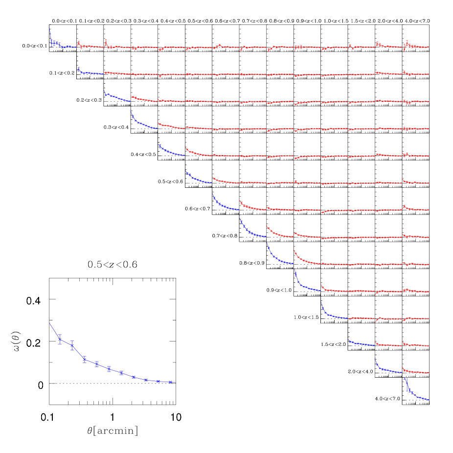
Furthermore, we also carried out a cross-correlation analysis of galaxies in photo-$z$ bins. The results can be found in the appendix A.

3 The LBG samples

3.1 Simulations

We simulate a colour catalogue of galaxies based on templates from the library of Bruzual & Charlot (1993) - in the same way as presented in Hildebrandt et al. (2007) for the ESO Deep Public Survey (DPS):

• We take the observed $i$-band number counts as a reference for creating the simulated colour catalogue.

• $i$-band magnitude-dependent and spectral-type-dependent redshift distributions are extracted from the BPZ code. These are based on catalogues extracted from the Hubble Deep Field North (Fernández-Soto et al., 1999) and the Canada-France Redshift Survey (Lilly et al., 1995).

• A huge multi-colour catalogue is simulated with the Hyperz (Bolzonella et al., 2000) photo-$z$ code evenly distributed in $i$-band magnitude, redshift, and spectral-type (eight different star-formation-histories applied to the library of Bruzual & Charlot, 1993).

• From this huge homogeneous catalogue we randomly pick objects for a given magnitude, type, and redshift bin. The numbers in a particular bin are scaled by the $i$-band number counts and the magnitude- and type-dependent redshift distributions mentioned above.

The colour catalogue simulated in this way shows very similar colour-colour diagrams as the observed catalogue (see also Hildebrandt et al., 2007) and is supposed to represent a realistic mix of galaxy types and low- and high-redshift objects.

In order to study the effect of the choice of the template set we re-run the simulations with the templates from Maraston et al. (2006) (see also Maraston, 2005) as a basis. In general, the results are very similar to the ones with the template set from Bruzual & Charlot (1993). The scientific results in this study are hardly affected by this choice. Nevertheless, we show results for both template sets in the remainder of the paper.

Furthermore, we simulate the colours of stars in our fields from the TRILEGAL galactic model (Girardi et al., 2005) taking into account the galactic coordinates of our survey fields and the depths of the images (see also Hildebrandt et al., 2007).

3.2 Selection

From these simulations we identify regions in colour-space where the efficiency of finding high-redshift star-forming galaxies is high due to their distinctive colours produced by the Lyman-break and where the contamination from low-redshift interlopers and stars is low. We do this in the $ugr$, $gri$, and $riz$ colour-spaces to select $u$-dropouts, $g$-dropouts, and $r$-dropouts, respectively. In Fig. 2 the fraction of objects in the desired redshift range ($u$-dropouts: $2<z<4$; $g$-dropouts: $3<z<5$; $r$-dropouts: $4<z<6$) is plotted as a function of colour. In order to steer away from the stellar locus, not the whole high-efficiency area in the $u-g$ vs. $g-r$ colour-space can be used.

Figure 2: Colour-colour diagrams showing the fraction of objects at the target redshifts (left: $2<z<4$; middle: $3<z<5$; right: $4<z<6$) as a function of colour in our simulations based on the templates from Bruzual & Charlot (1993), with black areas corresponding to 100% and white to 0% selection efficiency. The solid lines represent the selection criteria adopted in this study.

Figure 3: Same as Fig. 2 but based on the templates from Maraston et al. (2006) showing that the choice of the template set does not make any difference here.

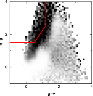
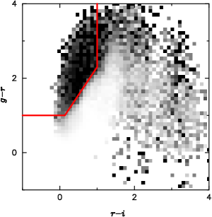
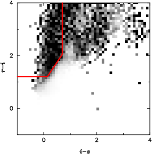
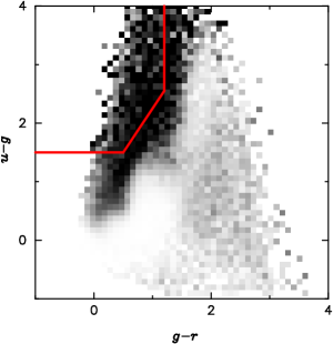
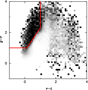
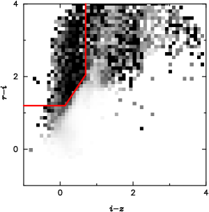
Our colour selection criteria are:

• for the $u$-dropouts: $1.5<(u-g)\>\wedge\>-1.0<(g-r)<1.2\>\wedge\>1.5\cdot(g-r)<(u-g)-0.75$ ,

• for the $g$-dropouts: $1.0<(g-r)\>\wedge\>-1.0<(r-i)<1.0\>\wedge\>1.5\cdot(r-i)<(g-r)-0.8$ ,

• for the $r$-dropouts: $1.2<(r-i)\>\wedge\>-1.0<(i-z)<0.7\>\wedge\>1.5\cdot(i-z)<(r-i)-1.0$ .

Furthermore, we require all LBGs to have a SExtractor CLASS_STAR parameter of $\mathrm{CLASS\_STAR}<0.9$, that $g$-dropouts are not detected in $u$, and that $r$-dropouts are neither detected in $u$ nor in $g$. In this way we select 34 218 $u$-dropouts, 36 226 $g$-dropouts, and 10 482 $r$-dropouts from the effective area of 3.17 sq. deg., i.e. the area after masking (see Erben et al., 2009, for a detailed description of the masking algorithms).

3.3 Properties

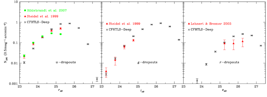
The number counts of the three samples are plotted in Fig. 4. They are in good agreement with previous studies, but the superior quality of the CFHTLS-Deep data for this kind of analysis is clearly visible, most dramatically for the $r$-dropout sample.

The number counts suggest approximate completeness limits of $r=25.5$ for the $u$-, $i=26.0$ for the $g$-, and $z=26.5$ for the $r$-dropouts. These completeness limits should not be regarded as robust. We only choose them by eye. Extensive simulations are prepared to quantify reliably the completeness as a function of magnitude. These are important for estimates of luminosity functions but are beyond the scope of this study, especially since the clustering measurements are not affected strongly by some low amounts of incompleteness.

From the simulated catalogues described above we find that the contamination from stars and low-$z$ interlopers can be kept below the 10% level in each magnitude bin (bin-size $\Delta\mathrm{mag}=0.5$) by applying a bright cutoff of $r>23$ for the $u$-, $i>23.5$ for the $g$-, and $z>24$ for the $r$-dropouts (for a discussion on how to avoid contaminants in an $R$-dropout survey by a bright cutoff see also Lehnert & Bremer, 2003). These magnitude cuts define our high-quality samples which consist of 17 338 $u$-, 17 281 $g$-, and 7038 $r$-dropouts. In the following, only LBGs in these magnitude ranges are considered.

Figure 4: Number counts for the three dropout samples ($u$-dropouts left, $g$-dropouts middle, and $r$-dropouts right) in the bands corresponding to approximately the same rest-frame UV-wavelength. We compare our $u$-dropout number counts to the ones from Steidel et al. (1999) and Hildebrandt et al. (2007) clearly showing the greater depth of the CFHTLS-Deep data. The $g$-dropout number counts are compared to Steidel et al. (1999) being consistent for $i<24.5$ and suggesting some incompleteness of the older survey for fainter magnitudes. The 13 $R$-dropouts reported in Lehnert & Bremer (2003) show a similar number density as the $r$-dropouts in the current study.

3.4 Redshift distributions

The redshift distributions of the LBG samples are of crucial importance in the physical interpretation of the angular clustering results presented below. There is virtually no overlap between the secure spectroscopic samples of the VVDS, zCOSMOS, and DEEP2 and our high-quality dropout samples. Nearly all LBG candidates are too faint and the brighter ones do not have good spectroscopic measurements as indicated by their spectroscopic flags. Here, we present four different ways to estimate the redshift distribution by other means. All four sets of redshifts distributions, which are displayed in Fig. 5, will be used in Sect. 4.2 to interpret the observed clustering.

3.4.1 Photo-$z$ distributions from BPZ

The photometric redshift distributions of the selected objects, estimated with BPZ and filtered for a BPZ ODDS parameter of ${\rm ODDS}>0.9$, show clear peaks at the targeted redshifts. The means and RMS-widths of these peaks are $z=3.28\pm 0.15$, $z=3.87\pm 0.32$, and $z=4.74\pm 0.14$. While the mean redshifts agree well with expectations, the widths of the distributions for the $u$- and the $r$- dropouts seem too small. This may well be an effect of the aggressive prior used by BPZ or the empirical template set, which is based on low-$z$ observations.

If we run BPZ without the prior, objects with a low ODDS parameter that were assigned a low redshift before are assigned a high redshift. This is exactly the behaviour one expects from double peaked redshift probability functions. For fixed ODDS the width of the $z$-distributions does not change from the prior- to the non-prior-setup. If the prior is switched off and additionally the cut on ${\rm ODDS}>0.9$ is dropped the $z$-distributions change only slightly.

It is the width of the redshift distribution rather than the mean redshift that is important for the interpretation of the clustering measurements (correlation lengths, galaxy bias, halo masses, and halo occupation numbers) described below.

3.4.2 Photo-$z$ distributions from Hyperz

An independent check of the photo-$z$’s with Hyperz and the template set based on the library of Bruzual & Charlot (1993) yields the following means and RMS-widths: $z=2.93\pm 0.24$ for the $u$-, $z=3.67\pm 0.31$ for the $g$-, and $z=4.47\pm 0.22$ for the $r$-dropouts. The distributions are shown in Fig. 5 as well. While the Hyperz RMS widths seem more realistic, the mean redshift values are slightly lower than the BPZ ones above and also lower than the theoretically expected ones. In Hildebrandt et al. (2008) we found that for a magnitude limited galaxy sample the photo-$z$’s for this particular combination of code and template set and estimated from a similar filter set ($UBVRI$) are biased low at the $\sim 5\%$ level when compared to spectroscopic redshifts of the VVDS. This is most probably due to a slight mismatch of the absolute spectrophotometric calibration of the templates and the absolute photometric calibration of the data. Correcting for this bias would make the mean redshifts of the $g$- and $r$-dropouts very compatible with BPZ leaving only the $u$-dropouts slightly low, although it is questionable whether this bias will remain constant out to much higher redshifts than probed by the VVDS.

The multi-modality of the photometric redshift distributions hints at problems in the photo-$z$ estimation. No such multi-modalities are observed in spectroscopic surveys of LBGs (see e.g. Steidel et al., 1999, 2003) nor are they expected theoretically. Thus, we regard the Hyperz redshift distributions as the least reliable ones.

3.4.3 Redshift distributions from simulations

The redshift distributions which are derived from the simulated colour catalogues are shown in Fig. 5 as well. The ones based on the templates from Bruzual & Charlot (1993) suggest mean redshifts and RMS-widths of $z=3.16\pm 0.22$ for the $u$-, $z=3.76\pm 0.30$ for the $g$-, and $z=4.73\pm 0.24$ for the $r$-dropouts. The simulations based on Maraston et al. (2006) templates yield means and widths of $z=3.30\pm 0.24$, $z=3.83\pm 0.32$, and $z=4.77\pm 0.24$ for the $u$-, $g$-, and $r$-dropouts, respectively.

Figure 5: Redshift distributions (arbitrarily normalised) of the three dropout samples ($u$-dropouts solid, $g$-dropouts dotted, and $r$-dropouts dashed). The first panel shows the BPZ photo-$z$ distributions, the second panel shows the Hyperz photo-$z$ distributions, the third panel shows the distributions derived from the simulated colour catalogue based on Bruzual & Charlot (1993) templates, and the last panel shows the distributions derived from the simulated colour catalogue based on Maraston et al. (2006) templates.

In the following we will refer to the four sets of redshift distributions as the BPZ, the Hyperz, the BC_sim, and the Maraston_sim distributions.

By choosing the $r$-band as the reference magnitude for the $u$-dropouts, the $i$-band for the $g$-dropouts, and the $z$-band for the $r$-dropouts we select galaxies at similar UV rest-frame wavelengths (mean rest-frame wavelength of the filters is $\sim 1560\AA$ for BC_sim) so that the $k$-correction between the different samples is negligible. The distance modulus between the mean redshifts of the $u$- and the $g$-dropouts and between the mean redshifts of the $g$- and the $r$-dropouts is $\sim 0.39$mag and $\sim 0.65$mag, respectively (again for BC_sim).

4 Clustering analysis

4.1 Technique

We estimate the angular correlation function $\omega(\theta)$ of the different flux-limited subsamples by applying the estimator of Landy & Szalay (1993). Errors are estimated from the field-to-field variance of the four fields. We choose a common angular binning for all samples but we check the influence of this choice (see below). The same masks as for the object detection are used for creating the random catalogue, which is necessary to estimate the correlation function. See Fig. 6 for the correlation functions of the different magnitude-limited LBG samples.

Figure 6: Angular correlation functions for the LBG samples of the three dropout populations ($u$-dropouts top, $g$-dropouts middle, and $r$-dropouts bottom) for different limiting magnitudes (corrected for the integral constraint bias with the BC_sim redshift distributions). The errors are estimated from field-to-field variance over the four CFHTLS-Deep fields. The solid lines represent power-law fits to the data in the angular region $0\aas@@fstack{\prime}1<\theta<10\arcmin$. For all samples we find a significant deviation on small scales from this power-law behaviour on larger scales.

We fit a power-law, $\omega(\theta)=A\,\theta^{-\delta}$, to the angular correlation functions in the angular region $0\aas@@fstack{\prime}1<\theta<10^{\prime}$. A de-projection with Limber’s equation (Limber, 1953) involving the redshift distributions shown above (see of Fig. 5) yields the real-space correlation functions approximated by a power-law, $\xi(r)=\left(\frac{r}{r_{0}}\right)^{-\gamma}$, with $r_{0}$ being the comoving correlation length and $\gamma=\delta+1$ being the slope of the correlation function. We correct iteratively for the integral constraint bias with the method explained in Adelberger et al. (2005). In this way we also estimate values for the large-scale galaxy bias factor, $b_{\rm gal}$:

$$b_{\rm gal}=\frac{\sigma_{8,g}}{\sigma_{8}(z)}\,.$$ (1)

The galaxy fluctuations in spheres of radius $8h^{-1}{\rm Mpc}$ can be estimated from the power law fit to the correlation function in the following way (Peebles, 1980):

$$\sigma_{8,g}=\frac{72\left(r_{0}/8h^{-1}{\rm Mpc}\right)^{\gamma}}{(3-\gamma)(4-\gamma)(6-\gamma)2^{\gamma}}\,,$$ (2)

whereas the corresponding DM fluctuations at redshift $z$, $\sigma_{8}(z)$, are calculated from theory.

4.2 Results

The results are summarised in Tables 2-5 and the dependence of different measured quantities on redshift, magnitude, and the assumed redshift distribution is visualised in Fig. 7. The errors for $r_{0}$ and $b_{\rm gal}$ in Fig. 7 are estimated in Monte Carlo realisations from the errors of the power-law fit. Therein, we assume uncorrelated Gaussian errors of the amplitude and the slope of the power-law. In the lower S/N domain the error introduced by the binning of the data becomes dominant over the fitting error. We add this contribution in quadrature, which is estimated from the scatter for many different binnings.

Table 2: Clustering measurements of the three dropout samples for different flux limits using the BPZ redshift distributions.

	$u$-dropouts; $z_{\rm mean}=3.28$
$r_{\mathrm{l}im}$	$n_{\rm g}$	$\gamma$	$r_{0}$	$b_{\rm gal}$	IC
	[$h^{3}{\rm Mpc}^{-3}$]		[$h^{-1}$Mpc]
24.5	$5.45\times 10^{-4}\pm 5.55\times 10^{-5}$	$1.85\pm 0.06$	$5.03\pm 0.35$	$3.39\pm 0.22$	0.0056
25.0	$1.58\times 10^{-3}\pm 1.59\times 10^{-4}$	$1.67\pm 0.03$	$3.47\pm 0.13$	$2.41\pm 0.08$	0.0028
25.5	$3.43\times 10^{-3}\pm 3.44\times 10^{-4}$	$1.60\pm 0.02$	$2.76\pm 0.08$	$2.01\pm 0.05$	0.0020
$i_{\mathrm{l}im}$	$g$-dropouts; $z_{\rm mean}=3.87$
25.0	$5.20\times 10^{-4}\pm 5.28\times 10^{-5}$	$1.95\pm 0.08$	$5.43\pm 0.39$	$4.24\pm 0.28$	0.0021
25.5	$1.32\times 10^{-3}\pm 1.33\times 10^{-4}$	$1.68\pm 0.08$	$4.64\pm 0.27$	$3.49\pm 0.17$	0.0014
26.0	$2.67\times 10^{-3}\pm 2.68\times 10^{-4}$	$1.71\pm 0.05$	$3.69\pm 0.13$	$2.87\pm 0.08$	0.0010
$z_{\mathrm{l}im}$	$r$-dropouts; $z_{\rm mean}=4.74$
25.5	$4.96\times 10^{-4}\pm 5.11\times 10^{-5}$	$2.07\pm 0.07$	$5.22\pm 0.38$	$5.00\pm 0.37$	0.0142
26.0	$1.18\times 10^{-3}\pm 1.19\times 10^{-4}$	$2.10\pm 0.07$	$4.07\pm 0.18$	$3.90\pm 0.19$	0.0086
26.5	$2.08\times 10^{-3}\pm 2.09\times 10^{-4}$	$2.08\pm 0.04$	$3.45\pm 0.10$	$3.25\pm 0.09$	0.0060

Table 3: Same as Table 2 but for the Hyperz redshift distributions.

	$u$-dropouts; $z_{\rm mean}=2.93$
$r_{\mathrm{l}im}$	$n_{\rm g}$	$\gamma$	$r_{0}$	$b_{\rm gal}$	IC
	[$h^{3}{\rm Mpc}^{-3}$]		[$h^{-1}$Mpc]
24.5	$5.19\times 10^{-4}\pm 5.29\times 10^{-5}$	$1.88\pm 0.07$	$5.94\pm 0.42$	$3.66\pm 0.15$	0.0025
25.0	$1.50\times 10^{-3}\pm 1.51\times 10^{-4}$	$1.68\pm 0.03$	$4.25\pm 0.13$	$2.63\pm 0.06$	0.0013
25.5	$3.27\times 10^{-3}\pm 3.28\times 10^{-4}$	$1.62\pm 0.02$	$3.43\pm 0.08$	$2.20\pm 0.02$	0.0009
$i_{\mathrm{l}im}$	$g$-dropouts; $z_{\rm mean}=3.67$
25.0	$5.05\times 10^{-4}\pm 5.13\times 10^{-5}$	$1.95\pm 0.08$	$5.64\pm 0.38$	$4.22\pm 0.26$	0.0021
25.5	$1.29\times 10^{-3}\pm 1.29\times 10^{-4}$	$1.68\pm 0.08$	$4.83\pm 0.30$	$3.46\pm 0.17$	0.0014
26.0	$2.60\times 10^{-3}\pm 2.61\times 10^{-4}$	$1.71\pm 0.05$	$3.83\pm 0.15$	$2.85\pm 0.10$	0.0010
$z_{\mathrm{l}im}$	$r$-dropouts; $z_{\rm mean}=4.47$
25.5	$9.80\times 10^{-4}\pm 1.01\times 10^{-4}$	$2.16\pm 0.08$	$3.66\pm 0.22$	$3.36\pm 0.23$	0.0031
26.0	$2.33\times 10^{-3}\pm 2.36\times 10^{-4}$	$2.17\pm 0.07$	$2.90\pm 0.67$	$2.61\pm 0.62$	0.0018
26.5	$4.10\times 10^{-3}\pm 4.13\times 10^{-4}$	$2.13\pm 0.05$	$2.46\pm 0.07$	$2.18\pm 0.08$	0.0013

Table 4: Same as Table 2 but for the BC_sim redshift distributions including halo model estimates.

	$u$-dropouts; $z_{\rm mean}=3.16$
$r_{\mathrm{l}im}$	$n_{\rm g}$	$\gamma$	$r_{0}$	$b_{\rm gal}$	IC	$\log\left<M_{\mathrm{halo}}\right>$	$\left<N_{g}\right>$
	[$h^{3}{\rm Mpc}^{-3}$]		[$h^{-1}$Mpc]			[$h^{-1}M_{\odot}$]
24.5	$4.17\times 10^{-4}\pm 4.24\times 10^{-5}$	$1.87\pm 0.07$	$6.16\pm 0.43$	$4.00\pm 0.26$	0.0036	$12.68_{-0.37}^{+0.20}$	$0.32\pm 0.27$
25.0	$1.21\times 10^{-3}\pm 1.21\times 10^{-4}$	$1.68\pm 0.03$	$4.39\pm 0.17$	$2.86\pm 0.09$	0.0018	$12.26_{-0.33}^{+0.19}$	$0.70\pm 1.02$
25.5	$2.62\times 10^{-3}\pm 2.63\times 10^{-4}$	$1.61\pm 0.02$	$3.54\pm 0.10$	$2.39\pm 0.05$	0.0013	$12.06_{-0.19}^{+0.13}$	$0.84\pm 0.66$
$i_{\mathrm{l}im}$	$g$-dropouts; $z_{\rm mean}=3.76$
25.0	$3.41\times 10^{-4}\pm 3.46\times 10^{-5}$	$1.94\pm 0.08$	$6.02\pm 0.43$	$4.57\pm 0.36$	0.0028	$12.39_{-0.13}^{+0.10}$	$0.45\pm 0.33$
25.5	$8.68\times 10^{-4}\pm 8.73\times 10^{-5}$	$1.68\pm 0.08$	$5.24\pm 0.30$	$3.78\pm 0.19$	0.0019	$12.17_{-0.07}^{+0.06}$	$0.65\pm 0.57$
26.0	$1.76\times 10^{-3}\pm 1.76\times 10^{-4}$	$1.70\pm 0.04$	$4.16\pm 0.16$	$3.12\pm 0.10$	0.0013	$12.08_{-0.06}^{+0.05}$	$0.48\pm 0.13$
$z_{\mathrm{l}im}$	$r$-dropouts; $z_{\rm mean}=4.73$
25.5	$2.27\times 10^{-4}\pm 2.34\times 10^{-5}$	$2.10\pm 0.07$	$7.10\pm 0.53$	$6.95\pm 0.57$	0.0108	$12.26_{-0.17}^{+0.12}$	$0.30\pm 0.18$
26.0	$5.40\times 10^{-4}\pm 5.46\times 10^{-5}$	$2.13\pm 0.07$	$5.53\pm 0.26$	$5.41\pm 0.29$	0.0066	$12.08_{-0.25}^{+0.16}$	$0.39\pm 0.26$
26.5	$9.49\times 10^{-4}\pm 9.56\times 10^{-5}$	$2.09\pm 0.04$	$4.71\pm 0.17$	$4.52\pm 0.17$	0.0046	$12.00_{-0.19}^{+0.13}$	$0.16\pm 0.20$

Table 5: Same as Table 2 but for the Maraston_sim redshift distributions.

	$u$-dropouts; $z_{\rm mean}=3.30$
$r_{\mathrm{l}im}$	$n_{\rm g}$	$\gamma$	$r_{0}$	$b_{\rm gal}$	IC
	[$h^{3}{\rm Mpc}^{-3}$]		[$h^{-1}$Mpc]
24.5	$3.86\times 10^{-4}\pm 3.93\times 10^{-5}$	$1.87\pm 0.07$	$6.19\pm 0.40$	$4.14\pm 0.26$	0.0035
25.0	$1.12\times 10^{-3}\pm 1.12\times 10^{-4}$	$1.68\pm 0.03$	$4.41\pm 0.15$	$2.96\pm 0.09$	0.0018
25.5	$2.43\times 10^{-3}\pm 2.43\times 10^{-4}$	$1.61\pm 0.02$	$3.55\pm 0.10$	$2.48\pm 0.05$	0.0012
$i_{\mathrm{l}im}$	$g$-dropouts; $z_{\rm mean}=3.83$
25.0	$3.10\times 10^{-4}\pm 3.15\times 10^{-5}$	$1.94\pm 0.08$	$6.26\pm 0.46$	$4.82\pm 0.33$	0.0028
25.5	$7.89\times 10^{-4}\pm 7.94\times 10^{-5}$	$1.68\pm 0.08$	$5.44\pm 0.28$	$3.95\pm 0.17$	0.0019
26.0	$1.60\times 10^{-3}\pm 1.60\times 10^{-4}$	$1.70\pm 0.04$	$4.32\pm 0.17$	$3.26\pm 0.11$	0.0013
$z_{\mathrm{l}im}$	$r$-dropouts; $z_{\rm mean}=4.77$
25.5	$2.12\times 10^{-4}\pm 2.19\times 10^{-5}$	$2.09\pm 0.07$	$7.09\pm 0.54$	$6.98\pm 0.56$	0.0110
26.0	$5.05\times 10^{-4}\pm 5.11\times 10^{-5}$	$2.12\pm 0.07$	$5.51\pm 0.27$	$5.43\pm 0.36$	0.0067
26.5	$8.88\times 10^{-4}\pm 8.94\times 10^{-5}$	$2.09\pm 0.04$	$4.70\pm 0.16$	$4.54\pm 0.16$	0.0046

Figure 7: Dependence of the correlation length, the correlation function slope, and the galaxy bias parameter on redshift, UV-luminosity, and the assumed redshift distribution. The solid lines and the crosses correspond to the $u$-dropouts, the dotted lines and the triangles to the $g$-dropouts, and the dashed lines and the squares to the $r$-dropouts, respectively. We scale the $r$- and $i$-band limiting magnitudes of the $u$- and $g$-dropouts to the $z$-band limits of the $r$-dropouts as described in the text.

There is clear evidence for clustering segregation with rest-frame UV luminosity for all three dropout samples regardless of the assumed redshift distribution. Brighter samples cluster more strongly than fainter ones as reflected by their correlation lengths and bias values.

The observation that the correlation function slope on intermediate and large scales gets shallower for fainter galaxies as reported by Ouchi et al. (2005), Kashikawa et al. (2006), and Hildebrandt et al. (2007) is also detected in our $u$- and $g$-dropout samples. Furthermore, we also detect a similar levelling-off of the slope for the two faintest bins as reported by Hildebrandt et al. (2007) for a $U$-dropout sample. The flattening of the correlation function for fainter magnitudes is not observed for the $r$-dropouts. They show a constant, rather steep slope of $\gamma\approx 2.1$ for all magnitude limits.

The measurement of correlation lengths is strongly dependent on the assumed redshift distributions which have not been spectroscopically verified. However, the $u$-dropout samples show smaller correlation lengths than the higher redshift samples for the BPZ, the BC_sim, and the Maraston_sim redshift distributions, indicating some evolution may be occurring.

A much clearer redshift dependence is observed for the values of the large-scale galaxy bias again for the BPZ, the BC_sim, and the Maraston_sim redshift distributions. From $z\sim 5$ to $z\sim 3$ the galaxy bias decreases by a factor of two. This more pronounced trend in comparison to the correlation lengths can easily be explained by the ongoing structure formation in the early universe. DM halos with roughly the same comoving correlation length are more biased tracers of the underlying dark matter field at high redshifts than at lower redshifts. This is due to the fact that the amplitudes of the overall DM density field grow with time. Thus, the scale where the correlation function takes a value of one (the correlation lengths) increases over time.

In Hildebrandt et al. (2007) we found clustering segregation with UV luminosity as well but the correlation lengths of that $U$-dropout sample were consistent with the ones from the $B$-dropout sample from Ouchi et al. (2005) for the same luminosity, showing no evolution with redshift. Besides the much larger statistical power of the present survey, it should be noted that several systematic effects can influence such a comparison of different datasets. For example, it is not clear whether intrinsically very similar populations were studied in Ouchi et al. (2005) and Hildebrandt et al. (2007) because of the different filter sets, the different selection criteria, and the different depths of the data. Furthermore, masking can introduce biases in the clustering signal that are hard to control. Most importantly (see above), the redshift distributions were obtained in very different ways with Hildebrandt et al. (2007) relying on Hyperz photo-$z$’s and Ouchi et al. (2005) on simulations. Indeed, the non-evolution of the correlation length with redshift from $z\sim 4$ to $z\sim 3$ is seen also here in the Hyperz panel in Fig. 7. It might well be spurious due to the problems mentioned in Sect. 3.4.2.

In the present study we carry out a coherent analysis on one dataset. The selection criteria are taken from the same set of simulations and the masking is identical for all three samples. However, without spectroscopic redshift distributions we cannot decide whether the evolutionary trend observed with the BPZ, the BC_sim, and the Maraston_sim redshift distributions or the non-evolution observed for the Hyperz redshift distribution is real. The simulated redshift distributions have the advantage that they are not affected by a number of systematic errors inherent to the observations (except for the reliance on the observed $i$-band number counts) or spurious effects introduced by priors in the photo-$z$ codes. Furthermore, the absolute results from the BC_sim case and the Maraston_sim case agree very well, although different template sets were used. One disadvantage of the simulations is that both rely on assumptions about the mixture of templates and the fractions of high- to low-$z$ objects which are taken from external data (the HDF-N and the CFRS). We tend to trust the results based on the simulated redshift distributions more, but note that a decision about redshift evolution or non-evolution cannot be taken without additional massive spectroscopic support.

The same is true for the influence of contamination or incompleteness on the clustering measurements. Without a deep spectroscopic survey we cannot account for such effects because we do not know how these possible low-$z$ contaminants cluster or which galaxies at high-$z$ are missed by the Lyman-break selection. This is a fundamental limitation of a photometric survey. However, our simulations suggest – and the colour selection criteria and magnitude cuts were chosen in such a way – that contamination and incompleteness are kept low. Thus, we still think it is reasonable to assume that the clustering measurements are not seriously affected by either of the two effects.

4.3 Halo model

As detected for $B$-dropouts (Ouchi et al., 2005; Lee et al., 2006) and $U$-dropouts (Hildebrandt et al., 2007) before, we see a significant deviation of the angular correlation function on small scales from the power-law behaviour on large scales for all three dropout samples. Especially, for the first time we detect this one-halo term contribution to the correlation function in our $r$-dropout sample at redshifts considerably larger than $z=4$. This allows us to fit a halo model to our data and estimate mean DM halo masses and occupation numbers (i.e. the mean number of galaxies hosted by a halo) for the different subsamples.

We apply the halo model with the same parameters as Hamana et al. (2004) which was used in several high-$z$ clustering studies before (e.g. in Ouchi et al., 2005; Hildebrandt et al., 2007). More advanced halo models are available (see e.g. Lee et al., 2008) but we decided to stick to the more simple one in order to keep our results comparable to older measurements. We only show the case for the BC_sim redshift distributions since the dependence of halo masses on the assumed redshift distribution is similar to the dependence of the correlation lengths and the galaxy bias values (see Sect. 4.2).

We fit for the mean galaxy density, $n_{\rm g}$, and the angular correlation function simultaneously. The mean galaxy density (also tabulated in Table 4) is estimated from the observed number of objects divided by the survey volume, the latter being estimated from the unmasked area and the redshift distribution. The error of the mean galaxy density is estimated from Poissonian variance of the galaxy numbers and from assuming a 10% error on the survey volume. We choose the angular fitting range for the halo models to $0\aas@@fstack{\prime}02<\theta<10^{\prime}$.

The inferred mean halo masses and mean halo occupation numbers for the different flux-limited subsamples are also listed in Table 4 and displayed in Fig. 8. Errors are again estimated from Monte-Carlo realisations assuming uncorrelated Gaussian errors on the halo model parameters $M_{\rm min}$, $M_{1}$, and $\alpha$, and we add the errors derived from the fluctuations introduced by the binning of the data.

Figure 8: Dependence of the mean halo mass and the mean halo occupation number on redshift, UV-luminosity for the BC_sim redshift distribution. Symbols and scalings same as Fig. 7

The halo masses for the three redshift samples are within errors nearly consistent with each other at fixed luminosity. While we see again a trend in the halo masses with luminosity in all three samples, a significant redshift dependence is not observed. Our data seem to favour the observation also made before by Hildebrandt et al. (2007) that lower redshift LBGs are hosted by more massive halos than higher redshift LBGs of the same rest-frame UV-luminosity. If this trend is real, the star-formation rate per unit mass decreases with redshift – at least in LBGs. This result is, however, highly dependent on the assumed redshift distribution. Taking e.g. the BPZ redshift distribution would further wash-out this already weak redshift evolution.

The mean halo occupation numbers are not very well constrained by the fit to the data but the trend that $\left<N_{g}\right><1$ for LBGs (as observed before by Ouchi et al. 2005 and Hildebrandt et al. 2007) is confirmed. The large errors seem to originate from some tension between the observed angular correlation functions and the observed number densities. This leads to only weak constrains on the $M_{1}$ parameter which is important to calculate $\left<N_{g}\right>$, whereas it does not influence the estimate of the $\left<M_{\rm halo}\right>$. A more elaborate method of calculating the errors on $\left<N_{g}\right>$ dropping the assumptions of Gaussianity and uncorrelated errors of the halo model parameters could potentially decrease uncertainties here.

Together with the observations of the strong one-halo term these occupation numbers mean that most halos of the mean mass reported here are devoid of LBGs and only a small number of them host a galaxy or a small group.

5 Conclusions

We carried out a precision analysis of LBG clustering at different redshifts from extremely deep optical imaging data in the CFHTLS-Deep fields. The LBG samples presented here are by far the largest studied so far. We detect a clear evolution of the large-scale galaxy bias and a tentative evolution of the correlation lengths with redshift for three of the four redshift distributions considered here. Higher-$z$ LBGs cluster more strongly than lower-$z$ ones. In agreement with former studies, we observe a strong trend with luminosity with brighter LBGs showing larger correlation lengths and galaxy bias values than fainter ones. Since the samples were selected from one dataset and the whole clustering analysis was done in a coherent way we can be confident that the relative comparisons are more accurate than comparisons carried out before which involved data from different sources. Also the absolute values of the correlation lengths, bias values, and slopes of the correlation functions are in good agreement to former studies considering the systematic difficulties arising from a redshift distribution based on simulations and the possible contribution of contaminants to the clustering signal (see also Stanway et al., 2008, for a detailed discussion of this aspect).

The common picture of LBGs forming in massive halos of $M\ga 10^{12}h^{-1}M_{\odot}$ is supported by our halo model analysis. Predictions from models of galaxy formation can be compared to ever more detailed observational results in this way. By detecting a significant one-halo term in the correlation function of $r$-dropouts for the first time, we have observational evidence for multiple galaxies hosted by single DM halos at very high redshifts.

In order to take this method to even higher precision and constrain models of galaxy formation and evolution even better the systematic errors must be better understood and controlled. A spectroscopic redshift distribution of representative subsamples is inevitable for reaching this goal. On the theoretical side one must think about more realistic models for galaxy clustering since this particular halo model used here is not a very good fit to the data, leaving considerable residuals. Lee et al. (2008) introduce interesting extensions to the halo model used here. We plan to incorporate information on the luminosity functions of the LBGs in a future study to learn more about the relationship between the star formation and the DM structure at high redshift. However, here we stuck to the simpler model to keep results comparable to older studies.

Appendix A Cross-correlation test of photo-$z$’s

Similar to Erben et al. (2009) we estimate the cross-correlation function of galaxies in photo-$z$ slices. In this way the null hypothesis of non-overlapping slices, which are far apart in redshift, can be tested. See Erben et al. (2009) for a detailed description of the technique. In Fig. 9 the auto- and cross-correlation functions of galaxies with $i<26.5$ in many different photo-$z$ slices are shown. The fact that nearly all cross-correlation functions of non-neighbouring photo-$z$ slices show an amplitude consistent or very close to zero is a strong argument for the robustness of the photo-$z$’s. No excessive overlap between low- and high-$z$ slices is observed. Thus, even for fainter magnitudes, the outlier rates are under control. A more quantitative analysis of this method will be presented in a forthcoming paper (Benjamin et al. 2009 in prep.).

Figure 9: Auto- (blue on the diagonal) and cross-correlation (red off-diagonal) functions of galaxies with $i<26.5$ in different photo-$z$ slices. The blow-up in the bottom left is just an example that illustrates the ranges of the axis.