The work by Finn et al further investigating our system is indeed relevant. Their results, particularly the complete absence of chaos for the $\Gamma=0.3$ case, are somewhat surprising and inconsistent with our results.

Our published results reported analysis on the in-principle experimentally accessible time-series. For $\Gamma=0.125$ Poincaré sections indicate a chaotic attractor at $\beta=0.01$, which is altered but persists for $\beta=0.3$ and disappears for $\beta=1$. For $\Gamma=0.3$, Poincaré sections show no chaos at $\beta=0.01$, an attractor for $\beta=0.3$, which disappears for $\beta=1$. The power spectra for $\langle\hat{X}(t)\rangle$ for all six cases agree with the above. Further, the $\beta=0.3$ results look extremely similar for the two $\Gamma$ cases.

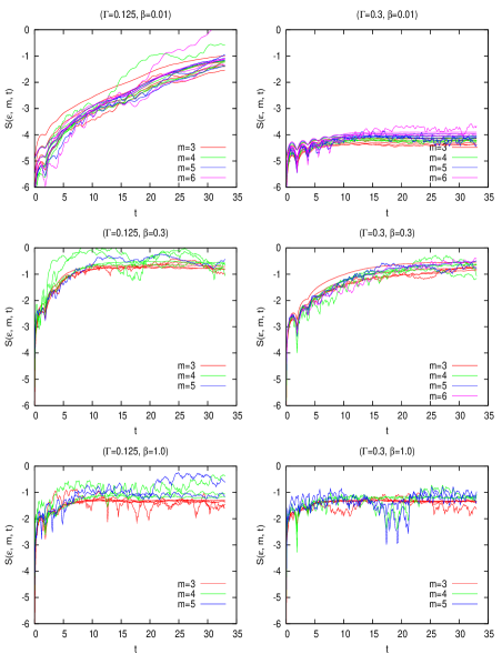
Figure 1: Each plot shows the divergence $S(\epsilon,m,t)=\ln(\Delta(t))$ of nearby points in the reconstructed phase space for a given $\Gamma,\beta$ pair. There are several curves in each plot with different delay embedding dimension $m$; for each $m$ there are curves corresponding to several different neighborhood radii $\epsilon$ in the reconstructed phase space. Exponential growth appears as linearity before the trajectories reach saturation; the slope is proportional to $\lambda$. See Ref. tisean for details on the technique.

We have since used the TISEAN packagetisean , performing phase-space delay reconstruction with $\langle\hat{X}(t)\rangle$ to obtain $\lambda$. We see qualitative agreement with our previous results (see Fig. (1)). We estimate $\lambda$ for respective $(\Gamma,\beta)$ pairs (approximately, since they derive from finding the slope of the straight line parts of these curves) as: $(0.125,0.01)\approx 0.1,(0.125,0.3)\approx 0.16,(0.125,1.0)<0.05,(0.3,0.01)<0.03,(0.3,0.3)\approx 0.13,(0.3,1.0)<0.05$. In short, this agrees with our previous conclusions about where chaos exists. Interestingly, using $\lambda$, the transition from quantum to classical behavior appears to be non-monotonic for both instances of $\Gamma$.

Our three methods of analysis (Poincaré sections, power spectra, and time-series Lyapunov exponents) are all consistent with each other, and consistent with our physical understanding of how the chaos emerges and/or is swamped by quantum effects. Finn et al’s calculation is inconsistent with this for the one ‘mesoscopic’ case of $(\Gamma,\beta)=(0.3,0.3)$ and we are particularly surprised that their results for the $(0.125,0.3)$ and $(0.3,0.3)$ cases are so different. As noted by an anonymous referee, it is possible that the chaos is a finite-time effect in a system where the infinite-time limit is non-chaotic. Of course, finite-time behavior is also physically important, and could be of greater physical relevance than the mathematical infinite-time limit in real experimental applications.

We expect that understanding the source of this difference — provided it is not due to technical errors — will reveal something deeper about the physics, or about the difference between the methods of analysis. Behind the immediate questions about the behavior of this model system stands the larger fundamental question of whether quantum corrections always regularize and suppress chaotic dynamics. We believe that this, while often true, is not universal. For the QSD equations (or equivalent stochastic Schrodinger equations) it is extremely unlikely that such a highly nonlinear equation has a priori a monotonic parameter landscape. Our perspective is supported, for example, by Bhattacharyya et al bhatt . It is only a matter of more systematic investigation to find other such counter-examples to the folklore.

Kyle Kingsbury^(a)

Chris Amey^(a)

Arie Kapulkin^(b)

Arjendu Pattanayak^(a)

(a) Department of Physics and Astronomy,
Carleton College, Northfield, Minnesota 55057
(b) 128 Rockwood Cr, Thornhill, Ont L4J 7W1 Canada

References

- (1) R. Hegger et al Chaos 9, 413 (1999); http://www.mpipks-dresden.mpg.de/~tisean/Tisean_3.0.1/index.html
- (2) T. Bhattacharya et al Phys. Rev. A65, 032115 (2002).