Long quantum transitions due to unstable semiclassical dynamics

Abstract

Quantum transitions are described semiclassically as motions of systems along (complex) trajectories. We consider the cases when the semiclassical trajectories are unstable and find that durations of the corresponding transitions are large. In addition, we show that the probability distributions over transition times have unusual asymmetric form in cases of unstable trajectories. We investigate in detail three types of processes related to unstable semiclassical dynamics. First, we analyze recently proposed mechanism of multidimensional tunneling where transitions proceed by formation and subsequent decay of classically unstable “states.” The second class of processes includes one–dimensional activation transitions due to energy dispersion. In this case the semiclassical transition–time distributions have universal form. Third, we investigate long–time asymptotics of transition–time distributions in the case of over–barrier wave packet transmissions. We show that behavior of these asymptotics is controlled by unstable semiclassical trajectories which linger near the barrier top.

1 Introduction

Semiclassical method unveils fascinating relation between the properties of quantum transitions and the character of classical dynamics of the system. This relation is valid, in particular, for tunneling processes [1] which do not exist at the classical level. Indeed, tunnelings are described semiclassically by complex trajectories [2] evolving classically in complex phase space. Observables characterizing tunneling processes, such as probabilities [2] or splittings of energy levels [3], are functionals of complex trajectories. Clearly, features of (complex) classical dynamics are imprinted in these observables.

The link between tunneling processes and classical dynamics is supported by theoretical studies of multidimensional tunneling. It was found that behavior of tunnel splittings of energy levels is qualitatively different for systems with integrable [4], near–integrable [5], mixed [6] and chaotic [7] dynamics. Some of the related phenomena have already been observed experimentally [8].

In this paper we study impact of non–trivial semiclassical dynamics on temporal characteristics of classically forbidden transitions. We are particularly interested in cases when complex trajectories describing transitions are unstable. Such trajectories do not interpolate directly between in– and out– regions of the process, but rather get attracted to a certain unstable orbit lying on the boundary between the regions. It takes large or even infinite time for a trajectory of this kind to arrive to the out–region. In general one does not expect the time scale of the semiclassical motion to coincide with the (properly defined) duration of quantum transition. Nevertheless, we advocate qualitative relation [9] between these quantities: durations of quantum processes are large when the corresponding semiclassical trajectories are unstable.

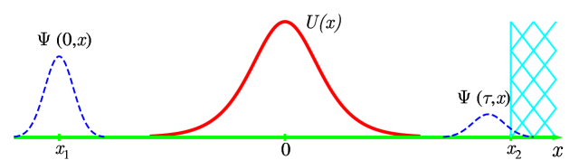
Figure 1: (Color online) Experimental setup for measuring the traversal–time distribution $\rho(\tau)$. Only the “transition” coordinate $x$ is shown. Macroscopic detector is represented by the hatched region $x>x_{2}$.

Presently there is no generally accepted definition of quantum traversal time [10]. During last decades a number of definitions have been suggested in literature [11, 12, 13, 14, 15]. Below we follow the approach of Refs. [16, 17, 18] where traversal time $\tau$ is treated as a random variable with probability distribution $\rho(\tau)$. Experiment for measuring $\rho(\tau)$ is depicted schematically in Fig. 1. The horizontal axis in this figure represents “transition” coordinate $x$ which runs between in– and out– regions of the process and meets potential barrier $U({\bf x})$ on the way. Quantum particle is emitted at $t=0$, $x\approx x_{1}$ in a definite initial state $\Psi_{i}({\bf x})=\Psi(0,{\bf x})$. As time goes on, the particle moves towards the potential barrier and eventually traverses it. At $t=\tau$ the particle is caught by the asymptotically distant macroscopic detector which occupies the region $x>x_{2}$ and registers the time of arrival $\tau$. The probability of registration is

$${\cal P}_{\tau}=\int\limits_{x>x_{2}}d{\bf x}_{f}\;|\Psi(\tau,{\bf x}_{f})|^{2}\;,$$ (1)

where the integration variable is denoted by ${\bf x}_{f}$ for later convenience. Note that the total transmission probability ${\cal P}_{\infty}$ is obtained from ${\cal P}_{\tau}$ in the limit $\tau\to+\infty$. We also remark that the points $x_{1}$ and $x_{2}$ are assumed to be far enough from the potential barrier, so that the particle moves freely at $x\lesssim x_{1}$, $x\gtrsim x_{2}$. One introduces the normalized probability density

$$\rho(\tau)=\frac{1}{{\cal P_{\infty}}}\frac{d{\cal P}_{\tau}}{d\tau}\;.$$ (2)

By construction, $\rho(\tau)\cdot d\tau$ is the increment of the registration probability, which is conditional with respect to the transition event. Following Refs. [16, 17, 18], we associate $\rho(\tau)$ with probability distribution over traversal times $\tau$. The average time of passing is then computed as

$$\langle\tau\rangle=\int_{0}^{+\infty}d\tau\;\tau\rho(\tau)\;,$$ (3)

and time dispersion $\sigma_{\tau}^{2}$ is defined accordingly.

It is worth noting that several assumptions about detector registering the particles have been made in Eq. (1). First, we adopted approximation of instantaneous measurements disregarding time resolution of the detector. Second, we assumed that the states of particles are not distorted prior to the measurement event. Third, our probability formula (1) is applicable only in the case of small registration probabilities: true probability of registering the particle at $t=\tau$ is conditional with respect to previous non–detection. For classically forbidden transitions considered below the probability of non–detection is close to $1$ and Eq. (1) is applicable. In other cases expression for ${\cal P}_{\tau}$ should be corrected [19].

Equipped with the definition (3), we study three examples of quantum processes related to unstable semiclassical trajectories. In all cases our results confirm the qualitative conclusion [9] about large transition times. Namely, we show that $\langle\tau\rangle\sim|\log g^{2}|$, $\sigma_{\tau}^{2}\gtrsim O(g^{0})$, where $g^{2}$ is the semiclassical parameter. In the limit of vanishingly small $g^{2}$ when the system becomes increasingly “more classical” the average duration of transition grows to infinity, while $\sigma_{\tau}^{2}$ stays finite or grows. This behavior is drastically different from the respective scalings in the case of stable trajectories where $\langle\tau\rangle$ reaches definite limit and $\sigma_{\tau}^{2}$ vanishes as $g^{2}\to 0$.

We consider the following classically forbidden processes. First and most importantly, we study tunneling transitions in non–linear multidimensional systems at high energies. Instability of semiclassical dynamics in this case was demonstrated in Refs. [20, 21], see Refs. [22] for earlier works. We have already sketched the behavior of the corresponding complex trajectories: they approach certain unstable orbit, remain close to it for an infinite time interval and then slide away into the out–region. In systems with two degrees of freedom the mediator unstable orbit describes periodic oscillations near the saddle point of the potential. We call it sphaleron or simply unstable periodic orbit. We also attribute instability of respective trajectories to appearance of new mechanism of sphaleron–driven tunneling (or tunneling driven by unstable periodic orbit). Recent studies [25, 26, 27] revealed two experimental signatures of this mechanism: the probabilities of related processes are suppressed by additional power–law factor [26] and distributions over out–state quantum numbers are anomalously wide [21, 26, 27]. Below we show that the distribution $\rho(\tau)$ and corresponding values of $\langle\tau\rangle$ and $\sigma_{\tau}^{2}$ can be used for experimental identification of the sphaleron–driven mechanism of tunneling.

Second, we investigate wave packet transmissions through one–dimensional potential barrier. We consider the case when the average energy of wave packet is lower than the height of the barrier but sufficiently close to it. Then transmission proceeds by activation caused by energy uncertainty in the initial state. The probability of such transmission is exponentially suppressed, while the corresponding semiclassical trajectory approaches the top of the barrier and stays there for an infinite time. This trajectory is unstable; its behavior is, again, of the type described above. Our calculations show that the forms of the semiclassical traversal–time distributions are universal in one dimension: all information about the potential barrier and initial wave packet is encoded in two parameters of the distributions, which can be absorbed by shifting and rescaling $\tau$. Universal forms of $\rho(\tau)$ lead to universal qualitative dependencies $\langle\tau\rangle\sim|\log g^{2}|$, $\sigma_{\tau}^{2}\sim O(g^{0})$ in the case of one–dimensional activation transitions.

Third and finally, we study the probabilities of large time delays $\tau$ in one–dimensional over–barrier transmissions. In this case the average energy of particle exceeds the height of the potential barrier. The particle is registered at time $\tau$ after transmission at a given distance behind the barrier; we calculate semiclassically the asymptotics $\tau\to+\infty$ of the registration probability. Semiclassical trajectories entering this calculation linger near the barrier top. The probability at large $\tau$ has universal form, again. Due to delays of the respective trajectories this probability is larger than one would expect naively.

We illustrate our findings by performing explicit calculations in systems with one and two degrees of freedom. In these systems we compare the semiclassical results for $\rho(\tau)$ with results of explicit quantum–mechanical calculations. We find agreement at small $g^{2}$.

The paper is organized as follows. We start in Sec. 2 with properties of traversal–time definition (3). Then, in Sec. 3 we discuss the mechanism of sphaleron–driven tunneling and one–dimensional activation processes. General semiclassical expression for $\rho(\tau)$ is introduced in Sec. 4. Results for the durations of quantum processes are presented in Sec. 5: we consider one–dimensional activation transitions in Sec. 5.1, investigate sphaleron–driven tunneling in Sec. 5.2 and study long–time asymptotics of “over–barrier” traversal–time distributions in Sec. 5.3. We summarize in Sec. 6. Details of semiclassical and exact quantum–mechanical calculations are presented in Appendices.

2 Properties of traversal–time definition

The controversial issue of quantum traversal time has attracted considerable attention during last decades [10]. The reason for the controversy seems to be hidden within the quantum theory itself which does not offer clear definition or unique method of computing the durations of quantum transitions. At the moment there exists a number of physically different definitions of quantum traversal time, see e.g. Refs. [11, 12, 13, 14, 15].

Expression (3) belongs to a wide class of definitions involving delay of the transmitted wave packet with respect to the incident one. In this approach the delay is computed using some feature of wave packet, maximum [11] or centroid [28]. In our case the probability conservation law implies that the distribution (2) is proportional to the total current through the surface $x=x_{2}$ at $t=\tau$. Thus, $\rho(\tau)$ reflects the form of the transmitted wave packet, and mean time of passing (3) fits into the above class of wave packet–related definitions. We remark that $\rho(\tau)\cdot d\tau$ can be regarded as a probability of registering the particle at time $\tau$ by the point–like detector situated at $x=x_{2}$.

The properties of the definition (3) are similar to those of other definitions from the same class. First, the setup used in the Introduction resembles recent experiments with photons [29, 30], and one can hope to measure the distribution $\rho(\tau)$ experimentally. Note, however, that experimental verification of our results, if possible, requires substantial modification of existing experiments. Indeed, recent measurements of traversal times have been performed in quasi–stationary regime where wave functions of particles are substantially wider than potential barriers. In this case the interval (3) coincides [28, 18] with the phase time of Bohm and Wigner [11] which is reproduced in actual measurements [29]. On the other hand, our results are obtained in the “semiclassical” case where the coordinate uncertainty is parametrically smaller than the barrier width.

Second, the interval (3) passes [18] self–consistency check of Refs. [10]: times of transmission through the barrier and reflection from it have sense of conditional averages over two mutually exclusive events.

Third, our traversal time (3) suffers from Hartman effect [31] which leads to superluminal velocities of under–barrier motions. This effect was observed experimentally [30]. It is explained as follows. One notices [10, 32] that the out–state of the tunneling process is formed by the waves constituting forward tail of the initial wave packet. Thus, the out–state is not related casually to the central part of the in–state wave function. On the other hand, only the central parts of in– and out– states contribute substantially into $\langle\tau\rangle$. Since casual connection between these parts is absent, apparent velocity $(x_{2}-x_{1})/\langle\tau\rangle$ can be superluminal. We stress that the definition (3) is sufficient for the purposes of this paper: we regard $\langle\tau\rangle$ as an experimentally measurable [30] quantity characterizing quantum transitions.

Finally, let us remark that quantum traversal time can be naturally defined without any reference to the delay between transmitted and incident wave packets: one can exploit stopwatches attached to the particle [13] or observe response of total transmission probability to the periodic modulation of the potential [14]. In these approaches the properties of traversal times are essentially different from those listed above. Although we believe that the qualitative conclusions of this paper should be valid for any reasonable setup, our quantitative results are not applicable for other traversal–time definitions.

3 Three processes

Let us describe three types of processes related to unstable semiclassical dynamics.

We start with one–dimensional activation transitions of quantum particles through potential barriers $U(x)$. In what follows we consider the setup in Fig. 1. The initial state $\Psi_{i}(x)$ is chosen to be a Gaussian wave packet with central position $x_{1}$, average momentum $p_{0}$ and momentum dispersion $\sigma_{p}^{2}$. Transmissions proceed between the in– and out– regions, $x\to-\infty$ and $x\to+\infty$ respectively. Points $x_{1}$ and $x_{2}$ in Fig. 1 belong to these regions.

We exploit the semiclassical approximation which is justified if

$$g^{2}\equiv\frac{\hbar}{l_{0}\sqrt{mV_{0}}}\ll 1\;.$$ (4)

Here $V_{0}$ and $l_{0}$ are height and width of the potential barrier and $m$ is the particle mass. Dimensionless parameter $g^{2}$ introduced in Eq. (4) measures accuracy of the semiclassical approximation; one can adjust the value of this parameter by changing $U(x)$. Below we adopt dimensionless units $m=\hbar=V_{0}/l_{0}^{2}=1$. In these units the height $V_{0}=1/g^{2}$ and width $l_{0}=1/g$ of the “semiclassical” barrier are parametrically large.

We use the following scalings of the in–state parameters with $g^{2}$. First, we suppose that the typical energy of the process is large, $p_{0}^{2}\sim V_{0}\sim 1/g^{2}$. Second, momentum dispersion is chosen to be of order one, $\sigma_{p}^{2}\sim O(g^{0})$. Finally, the points $x_{1}$ and $x_{2}$ are taken to be sufficiently far from the potential barrier, so that motion is free at $x\lesssim x_{1}$, $x\gtrsim x_{2}$. This implies $x_{1},\,x_{2}\sim 1/g$.

We have already mentioned in the Introduction that one–dimensional transmissions proceed by activation at some values of in–state parameters. Let us explain the origin of the effect by decomposing the initial state $\Psi_{i}$ in the basis of plane waves with fixed momenta $p$. We consider the case $p_{0}<p_{c,2}\equiv\sqrt{2V_{0}}$ when the initial wave packet is mostly formed by “under–barrier” modes with $p\sim p_{0}<\sqrt{2V_{0}}$. Clearly, these modes are exponentially suppressed after transmission. On the other hand, “over–barrier” modes with $p>\sqrt{2V_{0}}$ constitute exponentially small fraction of the initial state, but overcome the barrier with probability of order one. One sees that, depending on the suppressions, the probability ${\cal P}_{\infty}$ can be dominated by “under–barrier” or “over–barrier” modes. We call the respective transitions by tunneling and activation. Note that the value of ${\cal P}_{\infty}$ is exponentially suppressed in both cases. Note also that the activation processes are related to the possibility of overcoming the barrier due to finite momentum dispersion in the in–state.

In Sec. 5.1 we will argue that there always exists some critical value of momentum $p_{c,1}$ such that transitions proceed by activation in the region $p_{c,1}<p_{0}<p_{c,2}$. We will also demonstrate explicitly that activation transitions are described by unstable semiclassical trajectories which linger near the barrier top.

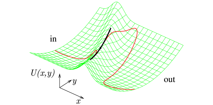
Figure 2: (Color online) Potential (5) (not to scale). On top of the potential surface: real part of complex trajectory (thin red line) describing sphaleron–driven tunneling at $gp_{0}=1.55$, $\sigma_{p}^{2}=0$, $g^{2}E_{y}=0.05$ and the sphaleron orbit (thick black line). The saddle point of the potential is shown with thick black dot.

The second type of processes is related to the multidimensional mechanism of sphaleron–driven tunneling. For definiteness we explain this mechanism in the model of Refs. [33, 20, 26] where two–dimensional quantum particle of mass $m$ moves in harmonic potential valley of frequency $\omega_{0}$. The valley is intersected at an angle by the potential barrier. The potential of the model is

$$U(x,y)=\frac{m\omega_{0}^{2}}{2}y^{2}+V_{0}\,\mathrm{e}^{-(x+y)^{2}/2l_{0}^{2}}\;,$$ (5)

where $V_{0}$ and $l_{0}$ are height and width of the barrier, respectively. Function $U(x,y)$ is plotted in Fig. 2.

Semiclassical approximation in the model (5) is justified under conditions (4) and

$$\omega\equiv\omega_{0}\,l_{0}\sqrt{m/V_{0}}\sim O(g^{0})\;.$$ (6)

In dimensionless units introduced above the potential (5) contains only two parameters, $g^{2}$ and $\omega$,

$$U(x,y)=\omega^{2}y^{2}/2+\frac{1}{g^{2}}\,\mathrm{e}^{-g^{2}(x+y)^{2}/2}\;.$$ (7)

We use $\omega=1/2$ for the waveguide frequency.

In what follows we study tunneling transitions between the asymptotic regions $x\to-\infty$ and $x\to+\infty$ (in– and out– regions respectively). In–states $\Psi_{i}$ of transitions are fixed completely by taking $\Psi_{i}(x,y)=\psi_{x}(x)\cdot\psi_{y}(y)$, where $\psi_{x}(x)$ is a Gaussian wave packet with central position $x_{1}$, average momentum $p_{0}$ and momentum dispersion $\sigma_{p}^{2}$, and $\psi_{y}(y)$ is an oscillator eigenfunction with energy $E_{y}$. We propagate semiclassically the in–state into the out–region and compute the probability ${\cal P}_{\infty}$ and traversal–time distribution $\rho(\tau)$.

In the semiclassical regime the typical energies of motion in $y$ direction are parametrically large, $E_{y}\sim 1/g^{2}$. The scalings of other parameters are chosen in the same way as in the above case of one–dimensional transitions. We characterize transitions with the combinations $gp_{0}$, $g^{2}E_{y}$, $\sigma_{p}^{2}$, $gx_{1}$, $gx_{2}$ which stay finite as $g^{2}\to 0$.

Note that transmissions between the asymptotic regions of the potential (7) remain classically forbidden even when the total energy $p_{0}^{2}/2+E_{y}$ exceeds the minimum height $V_{0}=1/g^{2}$ of the potential barrier. Indeed, classical trajectories with energies slightly higher than $V_{0}$ can overcome the barrier only by passing in the immediate vicinity of the saddle point of the potential. General trajectory misses this vicinity, and the corresponding transition remains classically forbidden. The probability of such transition is exponentially suppressed on general grounds. Tunneling transitions at energies exceeding the height of the potential barrier are known as dynamical tunneling [2, 34].

The mechanism of sphaleron–driven tunneling is based [20, 21] on behavior of complex trajectories in the regime of dynamical tunneling. One of such trajectories is depicted in Fig. 2 (thin red line). It overcomes the barrier in two stages, by approaching the unstable periodic orbit (sphaleron) and departing from it. Note that the sphaleron is real; it is plotted in Fig. 2 by thick black line. This orbit is unstable by construction, since it describes oscillations around the saddle point $x=y=0$ of the potential. The semiclassical trajectories in the new tunneling mechanism remain close to the sphaleron for an infinite time interval; imaginary parts of these trajectories become negligibly small after several sphaleron oscillations.

In general one finds that the sphaleron–driven mechanism is relevant in some region of in–state parameters, $p_{c,1}<p_{0}<p_{c,2}$, where $p_{c,1}$, $p_{c,2}$ are critical momenta depending on $E_{y}$ and $\sigma_{p}^{2}$. Regions of low and high momenta, $p_{0}<p_{c,1}$ and $p_{0}>p_{c,2}$ respectively, correspond to direct tunneling through the barrier and classical over–barrier transitions.

We remark that multidimensional processes of sphaleron–driven tunneling are essentially different from the one–dimensional activation transitions considered above: instability of trajectories in the sphaleron–driven case is not caused by finite momentum dispersion.

The third effect considered in this paper is related to the possibility of large time delays in over–barrier wave packet transmissions. For simplicity we return to one–dimensional setup where Gaussian wave packets traverse the potential barrier $U(x)$. Now, we are interested in the case of high initial momenta, $p_{0}>\sqrt{2V_{0}}$, when the central part of wave packet overcomes the barrier classically. We study the tail of $\rho(\tau)$ corresponding to large traversal times $\tau$. In Sec. 5.3 we will argue that this tail can be readily found by considering unstable semiclassical trajectories which linger near the barrier top.

From the physical viewpoint the origin of the effect is explained, again, by decomposing the initial state into a collection of plane waves with fixed asymptotic momenta $p$. In general, waves with $p\approx\sqrt{2V_{0}}$ are populated, although the respective probability is exponentially small. These waves get delayed near the top of the barrier and create long tail of $\rho(\tau)$.

4 Semiclassical method

Here we describe the standard method of complex trajectories [2] and introduce convenient semiclassical expression for $\rho(\tau)$. Although the semiclassical techniques of this Section are pretty general, we concentrate on the one– and two–dimensional models of Sec. 3.

For a start, let us briefly explain the origin of complex trajectories [2] leaving details of semiclassical computations to Appendix A. Consider evaluation of total transmission probability ${\cal P}_{\infty}$. One starts with the path integral for the final state,

$$\Psi(\tau,{\bf x}_{f})=\int d{\bf x}_{i}\,\Psi_{i}({\bf x}_{i})\int[d{\bf x}]\Big{|}_{{\bf x}_{i}}^{{\bf x}_{f}}\,\mathrm{e}^{iS[{\bf x}]}\;,$$ (8)

where the paths ${\bf x}(t)$ are defined in the time interval $t\in[0;\,\tau]$: they start at ${\bf x}(0)={\bf x}_{i}$ and arrive to ${\bf x}(\tau)={\bf x}_{f}$. $S[{\bf x}]$ is the action in this time interval. Since we are interested in ${\cal P}_{\infty}$, the value of $\tau$ will be sent to infinity in the end of calculation.

At small $g^{2}$ the integral (8) can be evaluated by the saddle–point method. Complex trajectory ${\bf x}(t)$ describing tunneling process is the saddle–point path of integration. In Appendix A we obtain saddle–point equations for this trajectory. Namely, ${\bf x}(t)$ should satisfy the classical equations of motion. Conditions at $t=0$ come from the saddle–point integration over ${\bf x}_{i}$,

$$\dot{x}_{i}-2i\sigma_{p}^{2}(x_{i}-x_{1})=p_{0}\;,\qquad\qquad E_{y}=(\dot{y}^{2}_{i}+\omega^{2}y^{2}_{i})/2\;,$$ (9)

where the subscript $i$ denotes quantities computed at $t=0$. [In the one–dimensional model of Sec. 3 only the first condition should be imposed.] One sees that the second of Eqs. (9) fixes initial energy of $y$–oscillator. Interpretation of the first equation is clear if the trajectory ${\bf x}(t)$ is real. In this case the real and imaginary parts of the first of Eqs. (9) constitute two independent conditions specifying the initial particle position $x_{i}=x_{1}$ and momentum $\dot{x}_{i}=p_{0}$. In the complex case the two parts are combined with the coefficient proportional to the momentum dispersion $\sigma_{p}^{2}$. Final boundary conditions for ${\bf x}(t)$ arise when one substitutes $\Psi(\tau,{\bf x}_{f})$ into the probability expression (1) and evaluates the saddle–point integral over ${\bf x}_{f}$. One obtains conditions

$$\mathrm{Im}\,\dot{\bf x}(t),\;\mathrm{Im}\,{\bf x}(t)\to 0\qquad\qquad\mbox{as}\qquad t\to+\infty$$ (10)

which mean that evolution in the out–region is real. Note that the limit $\tau\to+\infty$ is already taken in Eq. (10); at finite $\tau$ the integral over ${\bf x}_{f}$ cannot be evaluated by the saddle–point method.

After finding the trajectory ${\bf x}(t)$ from the classical equations of motion and boundary conditions (9), (10), one computes the transmission probability by the semiclassical formula

$${\cal P}_{\infty}=A\cdot\mathrm{e}^{-F/g^{2}}\;,$$ (11)

where the suppression exponent $F$ and prefactor $A$ are functionals of the saddle–point trajectory ${\bf x}(t)$. Explicit expressions for these functionals are derived in Appendices A and C, see Eqs. (37), (42) and (63).

Now, let us evaluate semiclassically the distribution $\rho(\tau)$. Following straightforward method [9], one should repeat the above considerations in the case of finite durations of transitions $\tau$ and apply Eqs. (1), (2). It is simpler, however, to use indirect technique introduced in Refs. [26].

With the purpose of explaining the logic of Refs. [26], we start from purely classical case when the traversal time $\tau$ is defined as the time of motion in the region $x<x_{2}$. [Recall that real classical trajectories start at $x=x_{1}$, $t=0$.] One introduces the functional

$$T_{int}[{\bf x}]=\int_{0}^{\infty}dt\,\theta(x_{2}-x(t))\;,$$ (12)

which returns traversal time for any classical path ${\bf x}(t)\in\mathbb{R}$. We call $T_{int}$ interaction time. To fix the value of $T_{int}$, one introduces Lagrange multiplier $\tilde{\epsilon}$ and changes the classical action, $S[{\bf x}]\to S[{\bf x}]+\tilde{\epsilon}(T_{int}[{\bf x}]-\tau)$. Trajectories ${\bf x}_{\tilde{\epsilon}}(t)$ extremizing the new action correspond to fixed durations $\tau=T_{int}[{\bf x}_{\tilde{\epsilon}}]$ of transitions. Note that the Lagrange method enables one to replace explicit fixation of traversal time $\tau$ with modification of classical equations of motion.

It is not trivial to introduce Lagrange method in quantum case. Indeed, there is no a priori reason to associate stochastic variable $\tau$ with values taken by the functional $T_{int}$. Still, we find that there exists close connection between these quantities. The technical trick revealing this connection is explained as follows. One inserts into the integrand of Eq. (8) the unity factor

$$1=\int_{0}^{\tau}d\tau^{\prime}\,\delta(T_{int}[{\bf x}]-\tau^{\prime})=\int_{0}^{\tau}d\tau^{\prime}\int_{i\infty}^{-i\infty}\frac{id\epsilon}{2\pi g^{2}}\;\mathrm{e}^{\epsilon(\tau^{\prime}-T_{int}[{\bf x}])/g^{2}}\;.$$ (13)

Since the paths ${\bf x}(t)$ in Eq. (8) are defined in the interval $t\in[0;\,\tau]$, we temporarily restrict integration in Eq. (12) to this interval. Now, $T_{int}[{\bf x}]$ takes values between $0$ and $\tau$; we explicitly used this fact in the first equality of Eq. (13). In the second equality we performed Fourier transformation and introduced “Lagrange multiplier” $\epsilon$. The path integral for $\Psi(\tau,{\bf x}_{f})$ takes the form,

$$\Psi(\tau,{\bf x}_{f})=\int_{0}^{\tau}d\tau^{\prime}\int_{i\infty}^{-i\infty}\frac{id\epsilon}{2\pi g^{2}}\left\{\int d{\bf x}_{i}\,\Psi_{i}({\bf x}_{i})\int[d{\bf x}]\Big{|}_{{\bf x}_{i}}^{{\bf x}_{f}}\,\mathrm{e}^{iS[{\bf x}]-\epsilon(T_{int}[{\bf x}]-\tau^{\prime})/g^{2}}\right\}\;.$$ (14)

Recall that the paths ${\bf x}(t)$ in this integral are defined in the interval $t\in[0;\,\tau]$. Expression (14) is remarkable in three respects. First, its integrand depends on ${\bf x}(t)$ via the new action $S[{\bf x}]+i\epsilon(T_{int}[{\bf x}]-\tau^{\prime})/g^{2}$ which is similar to the action arising in the classical Lagrange method. This is natural, since by inserting the $\delta$–function, Eq. (13), we introduced explicit constraint $T_{int}[{\bf x}]=\tau^{\prime}$ in the path integral. Second, apart from the modification of the action the integral in brackets in Eq. (14) has absolutely the same form as Eq. (8). Thus, it is evaluated in the same way as in Eq. (8), by finding the modified complex trajectory ${\bf x}_{\epsilon}(t)$. By construction, ${\bf x}_{\epsilon}(t)$ extremizes the modified action and satisfies the initial conditions (9).

The third favorable property of Eq. (14) is an explicit dependence of the integration limit on $\tau$. Let us schematically explain how this feature simplifies evaluation of the distribution $\rho(\tau)$. Recall that $\rho(\tau)$ is proportional to the derivative of ${\cal P}_{\tau}$ with respect to $\tau$, see Eq. (2). This derivative is evaluated easily if we represent ${\cal P}_{\tau}$ in the form ${\cal P}_{\tau}=\int_{0}^{\tau}d\tau_{+}\dots$, where $\tau_{+}$ is an integration variable, and the integrand does not depend on $\tau$. Then, $\rho(\tau)$ is simply proportional to the integrand of ${\cal P}_{\tau}$ taken at $\tau_{+}=\tau$.

We derive the desired integral for ${\cal P}_{\tau}$ in Appendix B. We start from Eq. (14) and perform all saddle–point integrations except for the integral over $\tau^{\prime}$ which is kept intact until the last moment. Then, we substitute $\Psi(\tau,{\bf x}_{f})$ into the probability expression (1) and integrate over ${\bf x}_{f}$. In this way we obtain ${\cal P}_{\tau}$ in the integral form, where $\tau$ explicitly enters the integration limits. At this stage the integrand of ${\cal P}_{\tau}$ is a functional of the modified trajectory ${\bf x}_{\epsilon}(t)$ which is defined in the interval $t\in[0;\,\tau]$. Using the modified equations of motion, we extend ${\bf x}_{\epsilon}(t)$ to $t\in[0;\,+\infty]$ and show that motion at $t>\tau$ does not contribute into the integrand of ${\cal P}_{\tau}$. In this way we show that the integrand does not depend on $\tau$. Thus, $\rho(\tau)$ is precisely the integrand of ${\cal P}_{\tau}$ at the end–point of integration; it is conveniently computed using the extended trajectory ${\bf x}_{\epsilon}(t)$, $t\in[0;\,+\infty]$.

The result of the derivation sketched above (see Appendix B for details) is summarized as follows. One starts by finding the modified trajectory ${\bf x}_{\epsilon}(t)$ which satisfies equations of motion following from the modified action

$$S_{\epsilon}[{\bf x}]=S[{\bf x}]+\frac{i\epsilon}{g^{2}}\,(T_{int}[{\bf x}]-\tau)$$ (15)

and old boundary conditions, Eqs. (9), (10). Importantly, ${\bf x}_{\epsilon}(t)$ is extended beyond the interval $t\in[0;\,\tau]$, and the final boundary conditions (10) are imposed at $t\to+\infty$. Then, we determine the saddle–point value of $\epsilon$. One can show that $\epsilon$ is real, so that the modification term in Eq. (15) is imaginary. This feature is specific to the case of classically forbidden transitions. Besides, $\epsilon$ is related to the duration $\tau$ by non–linear equation

$$\mathrm{Re}\,T_{int}[{\bf x}_{\epsilon}]=\tau\;,$$ (16)

which is similar to the respective constraint in the classically allowed case. We remark in passing that $\epsilon=0$ corresponds to the original complex trajectory ${\bf x}(t)$ which saturates the probability ${\cal P}_{\infty}$, see Eq. (15).

After finding the modified trajectory ${\bf x}_{\epsilon}(t)$ and solving Eq. (16) one computes the traversal–time distribution,

$$\rho(\tau)={\cal N}\sqrt{-\frac{d\epsilon}{d\tau}}\cdot A_{\epsilon}\,\mathrm{e}^{-F_{\epsilon}/g^{2}}\;,$$ (17)

where ${\cal N}$ is the normalization factor. Suppression exponent $F_{\epsilon}$ and prefactor $A_{\epsilon}$ in Eq. (17) are given by the same expressions as in Eq. (11), but with the modified action $S_{\epsilon}$ and modified trajectory ${\bf x}_{\epsilon}(t)$.

Note that the factor $A_{\epsilon}\cdot\exp(-F_{\epsilon}/g^{2})$ entering Eq. (17) has meaning of “naive” transition probability computed for the trajectory with action (15). The factor $\sqrt{-d\epsilon/d\tau}$ is not so trivial, however. From the technical viewpoint it arises due to fixation of $T_{int}$ in the path integral (8).

In what follows we exploit the relation which is derived in Appendix B,

$$2\epsilon=-dF_{\epsilon}/d\tau\;.$$ (18)

Equation (18) shows that the values of $\epsilon$ and $\tau$ are related by Legendre transformation. This is what one expects, since $\epsilon$ is interpreted as a Lagrange multiplier conjugate to $\tau$.

It is worth noting that the method of “Lagrange multipliers” introduced above resembles the approach of Refs. [15]. Note, however, one important difference: we define traversal–time distribution $\rho(\tau)$ by Eq. (2) and then introduce the functional $T_{int}[{\bf x}]$ as a convenient technical tool for the semiclassical calculation of this distribution. The authors of Refs. [15] go the other way around. They start with the functional similar to Eq. (12) and then define traversal time using path integral technique.

Let us mention one important restriction of the semiclassical method of this Section. While deriving Eq. (17) we assumed that only one complex trajectory gives substantial contribution into $\rho(\tau)$. This assumption is certainly correct for one–dimensional conservative systems; explicit calculations show that it also holds in the two–dimensional model (7). In other multidimensional systems [9] there might exist several (or even an infinite number of) trajectories giving comparable contributions into the traversal–time distribution. In this case Eq. (17) should be modified: contributions of different trajectories and respective interference terms should be accounted for.

We finish this Section by considering the standard tunneling mechanism where the original complex trajectory ${\bf x}(t)$ is stable. We are going to show that in this case $\rho(\tau)$ is symmetric and sharply peaked around the central value $\tau=\langle\tau\rangle$. From the Legendre transformation (18) one sees that the exponent $F_{\epsilon}$ in Eq. (17) has minimum at $\epsilon(\tau)=0$. This point corresponds to the original trajectory ${\bf x}(t)$. Since ${\bf x}(t)$ is stable, the respective value of $\tau=\mathrm{Re}\,T_{int}[{\bf x}]$ is finite. One expands the exponent around the point $\epsilon(\tau)=0$ and obtains the Gaussian distribution,

$$\rho_{s}(\tau)=\frac{1}{\sigma_{\tau}\sqrt{2\pi}}\cdot\mathrm{e}^{-(\tau-\langle\tau\rangle)^{2}/2\sigma_{\tau}^{2}}\;,$$ (19)

where we restored the normalization factor and added subscript $s$ (for “stable”). The central value $\langle\tau\rangle$ and dispersion $\sigma_{\tau}^{2}$ of this distribution are given by the expressions

$$\langle\tau\rangle=\mathrm{Re}\,T_{int}[{\bf x}]\sim O(g^{0})\;,\qquad\qquad\sigma_{\tau}^{2}=-\frac{g^{2}}{2}\frac{d\tau}{d\epsilon}\Bigg{|}_{\epsilon=0}\sim O(g^{2})$$ (20)

which come from the Taylor series expansion of the semiclassical exponent and Eqs. (16), (18). We remark that Eq. (19) is applicable at $|\tau-\langle\tau\rangle|\sim g$ where $\rho(\tau)\sim 1$. Outside of this region the value of $\rho(\tau)$ is negligibly small. Note also that the average duration $\langle\tau\rangle$ in Eqs. (20) is equal to the time spent by the original complex trajectory at $x<x_{2}$.

The above considerations are not valid if the original trajectory ${\bf x}(t)$ is unstable. In that case the point $\epsilon=0$ corresponds to $\tau=+\infty$ and the semiclassical exponent in Eq. (17) remains almost constant as $\tau\to+\infty$. Thus, $\rho(\tau)$ is essentially asymmetric: at large $\tau$ it falls off slowly, only due to prefactor. In the next Section we will show that the corresponding values of $\langle\tau\rangle$ and $\sigma_{\tau}^{2}$ are large.

5 Results

In this Section we compute distributions $\rho(\tau)$ for three quantum processes related to unstable semiclassical dynamics.

5.1 One dimension

We begin by considering one–dimensional activation transitions introduced in Sec. 3. For definiteness we suppose that the potential $U(x)$ reaches its maximum at $x=0$. We denote by $\omega_{-}^{2}=-U^{\prime\prime}(0)$ the curvature of the potential at the maximum. Note that $\omega_{-}$ stays finite as $g^{2}\to 0$. We will also use the exemplary potential

$$U(x)=\frac{1}{g^{2}\,\mathrm{ch}^{2}(gx)}$$ (21)

for checking and illustrating the semiclassical technique.

Let us show that the semiclassical dynamics is unstable in the case of activation transitions. We use the logic of Sec. 3 and decompose the initial state $\Psi_{i}$ in the basis of plane waves with fixed momenta $p$. Denoting by ${\cal P}_{p}$ the transmission coefficients of individual waves, we write,

$${\cal P}_{\infty}=\int_{0}^{\infty}dp\;{\cal P}_{p}\cdot|\Psi_{i}(p)|^{2}=\int_{0}^{\infty}dp\;{\cal P}_{p}\cdot\frac{1}{\sigma_{p}\sqrt{2\pi}}\;\mathrm{e}^{-{(p-p_{0})^{2}}/{2\sigma_{p}^{2}}}\;,$$ (22)

where interference terms are absent due to conservation of energy $E_{p}=p^{2}/2$. Recall that the value of $p_{0}$ is smaller than $p_{c,2}\equiv\sqrt{2V_{0}}$. On the other hand, the integration momentum $p$ in Eq. (22) can be higher or lower than $\sqrt{2V_{0}}$ representing the “over–barrier” or “under–barrier” modes, respectively. We consider these cases separately. Transmissions at $p>\sqrt{2V_{0}}$ are described by classical over–barrier trajectories. Thus, ${\cal P}_{p}=1$ and the integrand in Eq. (22) decreases with $p$ at $p>\sqrt{2V_{0}}$ due to the in–state contribution.

At $p<\sqrt{2V_{0}}$ the situation is different, since the coefficients ${\cal P}_{p}$ are exponentially suppressed. The semiclassical expression for these coefficients is well–known, ${\cal P}_{p}=\mathrm{exp}[-S(E_{p})]$ where $S(E_{p})$ is Euclidean action computed for one period of Euclidean oscillations in the upside–down potential. The semiclassical trajectory $x(t)$ performing oscillations has energy $E_{p}=p^{2}/2$. Let us visualize how $x(t)$ moves between the in– and out– asymptotic regions. In the in–region the trajectory evolves in real time until it stops at the left turning point of the potential. The subsequent semiclassical evolution proceeds in Euclidean time where $x(t)$ performs precisely one half–period oscillation in the upside–down potential. At the end of oscillation the trajectory arrives at the right turning point. After that $x(t)$ moves in real time, again, and finally ends up in the out–region. Only the Euclidean part of $x(t)$ contributes into ${\cal P}_{p}$.

One sees that for under–barrier modes both factors in the integrand of Eq. (22) are exponentially sensitive to the momentum $p$. To understand the behavior of the integrand, we consider its logarithmic derivative,

$$\frac{d}{dp}\mathrm{ln}\left[{\cal P}_{p}|\Psi_{i}(p)|^{2}\right]=p\,T(E_{p})-\frac{p-p_{0}}{\sigma_{p}^{2}}\;,$$ (23)

where $T(E)=-dS/dE$ is the period of Euclidean oscillations. Now, we take the limit $p\to\sqrt{2V_{0}}$ in Eq. (23). In this limit $E_{p}$ approaches the height of the potential barrier, and Euclidean oscillations get restrained to a small region near the barrier top. Thus, $T\to 2\pi/\omega_{-}$. Using this property, one finds that the derivative (23) is positive at $p=\sqrt{2V_{0}}$ if $p_{0}>p_{c,1}$, where

$$p_{c,1}=\sqrt{2V_{0}}\,(1-2\pi\sigma_{p}^{2}/\omega_{-})$$ (24)

is the critical momentum. Note that in the limit $E_{p}\to V_{0}$ the semiclassical trajectory $x(t)$ becomes unstable: it starts in the in–region and ends up on top of the potential barrier as $t\to+\infty$.

Now, one recalls that the integrand in Eq. (22) decreases with $p$ at $p>\sqrt{2V_{0}}$. Thus, it has sharp maximum at $p=\sqrt{2V_{0}}$ whenever $p_{0}$ lies between $p_{c,1}$ and $p_{c,2}\equiv\sqrt{2V_{0}}$. Moreover, this maximum is global if $T(E)$ decreases with energy, see Eq. (23). Thus, at $p_{c,1}<p_{0}<p_{c,2}$ the integral for the transmission probability ${\cal P}_{\infty}$ is saturated at $E_{p}=V_{0}$, i.e. precisely in the vicinity of unstable semiclassical trajectory.

The above considerations deserve two remarks. First, one can show that the semiclassical trajectory saturating the probability (22) satisfies the boundary conditions of the previous Section, Eqs. (9), (10). This is natural, since Eqs. (9), (10) are obtained from the requirement that the probability is extremal, see Appendix A. In Appendix C we explicitly solve the semiclassical equations in the model (21) and find the trajectory $x(t)$. It is unstable if $p_{c,1}<p_{0}<p_{c,2}$.

Second, the interval of unstable motions is semiclassically large, $p_{c,2}-p_{c,1}\sim 1/g$, and shrinks to a point as $\sigma_{p}^{2}\to 0$. This means that unstable semiclassical dynamics is essential in the case $g^{2}\ll 1$, $\sigma_{p}^{2}\sim 1$ which we consider.

Let us compute $\rho(\tau)$ in the case of unstable semiclassical trajectories $x(t)$. We have learned that such trajectories do not interpolate between the in– and out– regions of the process, but start in the in–region at $t=0$ and approach exponentially the barrier top $x=0$ as $t\to+\infty$. At large times one writes $x(t)=c_{-}\mathrm{e}^{-\omega_{-}t}$, where $c_{-}$ is a complex constant. Following the method of the previous Section, we introduce modification, Eq. (15). We will restrict attention to the case of small $\epsilon$ which will be important for calculating $\rho(\tau)$. One notes that the modified trajectory $x_{\epsilon}(t)$ moves in the complex potential

$$U_{\epsilon}(x)=U(x)-\frac{i\epsilon}{g^{2}}\,\theta(x_{2}-x)\;.$$ (25)

It cannot stop at the barrier top due to conservation of energy, which is real by Eqs. (10). The evolution described by $x_{\epsilon}(t)$ proceeds in three stages: the trajectory arrives into the region $x\approx 0$, spends some time there and then departs for the out–region. The modification term can be neglected during the first and last stages of evolution, but destroys unstable motion near the barrier top. Indeed, at $x_{\epsilon}\approx 0$ one writes,

$$x_{\epsilon}(t)=c_{-}\,\mathrm{e}^{-\omega_{-}t}+\epsilon c_{+}\,\mathrm{e}^{+\omega_{-}t}\;,$$ (26)

where $\epsilon$ in the second term reflects the fact that the original trajectory is recovered in the limit $\epsilon\to 0$. Since $\epsilon\ll 1$, the time of motion near the barrier top is large, and one computes $T_{int}$, Eq. (16), using the evolution (26),

$$\tau=-\frac{1}{\omega_{-}}\mathrm{ln}(\epsilon/\epsilon_{0})+O(\epsilon)\;,$$ (27)

where $\epsilon_{0}\sim O(g^{0})$ is some constant. In practice one finds the value of this constant explicitly, by obtaining the trajectory at all three stages of the modified evolution and calculating $T_{int}[x_{\epsilon}]$. Given $\epsilon(\tau)$, one computes the suppression exponent from Eq. (18),

$$F_{\epsilon}=F_{\infty}+2\int_{\tau}^{+\infty}d\tau^{\prime}\,\epsilon(\tau^{\prime})=F_{\infty}+\frac{2\epsilon_{0}}{\omega_{-}}\mathrm{e}^{-\omega_{-}\tau}\;,$$

where $F_{\infty}$ is independent of $\tau$.

Now, we estimate the modified prefactor $A_{\epsilon}$ at $\epsilon\ll 1$. The procedure for evaluating $A_{\epsilon}$ is described in Appendix C; we proceed by following this procedure in the case of small $\epsilon$. One finds the perturbation $\psi_{\epsilon}(t)$ which satisfies the linearized equations of motion in the background of the modified trajectory $x_{\epsilon}(t)$. Boundary conditions for $\psi_{\epsilon}(t)$ are imposed in the out–region. Evolving the perturbation back in time, one notes that $\psi_{\epsilon}(t)$ grows exponentially during the second stage of the modified evolution, Eq. (26). Thus, it becomes exponentially large at $t=0$, $\psi_{\epsilon}(0)\sim\mathrm{exp}(\omega_{-}\tau)$. At $\epsilon\ll 1$ the prefactor is estimated as $A_{\epsilon}\sim[\psi_{\epsilon}(0)]^{-1/2}$, see Eq. (63) of Appendix C. One finds $A_{\epsilon}\sim\mathrm{exp}(-\omega_{-}\tau/2)$.

Substituting $\epsilon(\tau)$, $F_{\epsilon}$ and $A_{\epsilon}$ into Eq. (17), we obtain the distribution

$$\rho_{u}(\tau)=\frac{2\epsilon_{0}}{g^{2}}\,\mathrm{exp}\left\{-\omega_{-}\tau-\frac{2\epsilon_{0}}{g^{2}\omega_{-}}\,\mathrm{e}^{-\omega_{-}\tau}\right\}\;,$$ (28)

which has the form of Gumbel distribution of type I [35]. We will argue below that Eq. (28) is valid in the region $\tau\gg|\log\epsilon_{0}|/\omega_{-}$ where $\rho_{u}(\tau)$ is not exponentially small. By using the subscript $u$ in the notation $\rho_{u}(\tau)$ we stress that Eq. (28) is valid in the case of unstable semiclassical trajectories.

Several remarks are in order. First, $\rho_{u}(\tau)$ is drastically different from the respective Gaussian distribution (19) which is valid in the case of stable semiclassical trajectories. Indeed, function (28) is essentially asymmetric. Besides, it corresponds to large mean time of transmission and large time dispersion,

$$\langle\tau\rangle=\frac{1}{\omega_{-}}\mathrm{ln}\left[\frac{2\epsilon_{0}}{g^{2}\omega_{-}}\right]+\frac{\gamma}{\omega_{-}}\;,\qquad\qquad\sigma_{\tau}^{2}=\frac{\pi^{2}}{6\omega_{-}^{2}}\;,$$ (29)

where $\gamma$ is the Euler constant. The quantities (29) depend on the semiclassical parameter as $\langle\tau\rangle\sim|\log g^{2}|$, $\sigma_{\tau}^{2}\sim O(g^{0})$, in contrast to the respective scalings $\langle\tau\rangle\sim O(g^{0})$, $\sigma_{\tau}^{2}\sim g^{2}$ in the case of stable trajectories, cf. Eqs. (20).

Second, the form of the distribution (28) is universal. Indeed, in deriving $\rho_{u}(\tau)$ we did not use any information about the potential $U(x)$ or initial wave packet $\Psi_{i}(x)$. All this information is encoded in two parameters of the distribution, $\epsilon_{0}$ and $\omega_{-}$. Moreover, one represents Eq. (28) in the form

$$\rho_{u}(\tau)=\omega_{-}\exp\left\{-\omega_{-}(\tau-\langle\tau\rangle)-\gamma-\mathrm{e}^{-\omega_{-}(\tau-\langle\tau\rangle)-\gamma}\right\}\;,$$

where the first of Eqs. (29) was used. All parameters in this formula disappear after appropriate shifts and rescalings of $\tau$.

Third, during the derivation of Eq. (28) we assumed that $\epsilon\ll 1$. This is legitimate at $\tau\gg|\log\epsilon_{0}|/\omega_{-}$, see Eq. (27). In particular, the region $\rho_{u}(\tau)\sim 1$ corresponds to $\tau\sim\langle\tau\rangle$ which leads to $\epsilon\sim g^{2}$, cf. Eqs. (29) and (27).

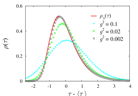
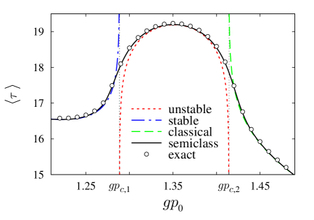
         (a)                                                                  (b)

Figure 3: (Color online) (a) One–dimensional traversal–time distributions in the case of unstable semiclassical dynamics. Points and solid line represent exact quantum mechanical results and Eq. (28), respectively. (b) Average time of passing in the model (21); $g^{2}=0.002$, $\sigma_{p}^{2}=0.02$, $gx_{2}=-gx_{1}=10$.

We derived expression (28) using the properties of the modified semiclassical dynamics. This expression is illustrated in Appendix C where we compute $\rho(\tau)$ for the model (21). In the region $p_{c,1}<p_{0}<p_{c,2}$ the result of Appendix C coincides with Eq. (28), where

$$\epsilon_{0}=\sin\left[\frac{\sqrt{2}-gp_{0}}{2\sigma_{p}^{2}}\right]\cdot\mathrm{e}^{g(x_{2}-x_{1})}\;.$$ (30)

Note that $\epsilon_{0}$ vanishes at $p=p_{c,1}$ and $p=p_{c,2}\equiv\sqrt{2}/g$, see Eq. (24). Function (28) is depicted in Fig. 3a, solid line.

As a check of the modified semiclassical method, we compare $\rho_{u}(\tau)$ with exact quantum mechanical results (points in Fig. 3a). The latter results are obtained by propagating numerically wave packets in the model (21) and using Eqs. (1), (2). One sees that the exact graphs are almost symmetric at large $g^{2}$ but change their form and approach $\rho_{u}(\tau)$ as $g^{2}\to 0$.

Our semiclassical expressions for the average time of passing are summarized in Fig. 3b which displays dependence of $\langle\tau\rangle$ on $p_{0}$ in the model (21). The interval of unstable semiclassical motions $p_{c,1}<p_{0}<p_{c,2}$ is delimited on the graph by the vertical dotted lines. The regions to the left and to the right of this interval correspond to stable tunneling trajectories and classical over–barrier solutions, respectively. In accordance with the above discussion, we compute $\langle\tau\rangle$ by Eq. (29) in the central part of the plot and by Eq. (20) in the rest of it. The corresponding dependencies are marked in Fig. 3b as “unstable”, “stable” and “classical”. All three graphs exhibit unphysical behavior in the vicinities of critical momenta $p_{c,1}$, $p_{c,2}$, where the “stable” and “classical” curves grow to infinity, and “unstable” graph sharply drops down. This behavior is related to “phase transition” which transforms stable trajectories into unstable and Gaussian distribution (19) into Eq. (28). Near the critical points $\langle\tau\rangle$ is computed with the full semiclassical distribution (17). This calculation is performed in Appendix C. In Fig. 3b we show the result by the solid line which smoothly interpolates between the “stable”, “unstable” and “classical” graphs and coincides with the average time of passing extracted from the exact quantum mechanical calculations (points).

5.2 Two dimensions

We proceed by considering the case of sphaleron–driven transitions in the two–dimensional model of Sec. 3. At the level of complex trajectories these transitions look similar to one–dimensional activation processes of the previous Section. However, there is one important difference: the origin of semiclassical instabilities in the sphaleron–driven case is related to non–linear interaction between the degrees of freedom, rather than to the momentum dispersion in the initial state. Recall that the new mechanism is relevant in the region $p_{c,1}<p<p_{c,2}$, where $p_{c,1}$ and $p_{c,2}$ are critical momenta defined in Sec. 3.

In the semiclassical calculations of this Section we use numerical methods of Refs. [33, 26]. Namely, we smoothen the step–function in the modified potential, Eq. (25),

$$\theta(x)\to\theta_{a}(x)=\frac{1}{1+\mathrm{e}^{-x/a}}\;,$$

where the width $a$ is supposed to be small. After that we introduce non–uniform lattice $t\in\{t_{k}|\,k=1\dots N_{k}\}$. The trajectory ${\bf x}_{\epsilon}(t)$ is found from the modified equations of motion and boundary conditions (9), (10) in the discrete case. Then, the values of $F_{\epsilon}$, $A_{\epsilon}$ and $\rho(\tau)$ are computed by Eqs. (37), (42) of Appendix A and Eq. (17), respectively.

We start with the simplified case when the total energy $E$ of the original sphaleron–driven trajectory ${\bf x}(t)$ is close to the height of the barrier, $E-V_{0}\ll V_{0}$. The sphalerons with these energies describe small linear oscillations around the saddle point $x=y=0$ of the potential; for the modified semiclassical motion in the vicinity of the saddle point one writes,

$${\bf x}_{\epsilon}(t)={\bf x_{-}}\left(c_{-}\mathrm{e}^{-\omega_{-}t}+\epsilon c_{+}\mathrm{e}^{\omega_{-}t}\right)+{\bf x_{+}}c\cos(\omega_{+}t+\varphi)\;,$$ (31)

cf. Eq. (26). Vectors ${\bf x}_{+}$ and ${\bf x}_{-}$ in this expression run along “stable” and “unstable” directions of the saddle point, while $\omega_{\pm}$ represent respective “frequencies.” Using the same arguments as in the previous Section, one shows that the distribution $\rho(\tau)$ is given by Eq. (28) if Eq. (31) is justified (i.e. at $E-V_{0}\ll V_{0}$).

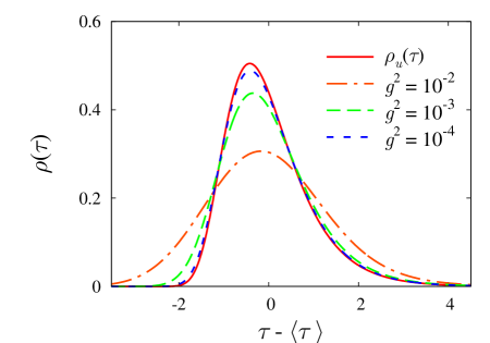
Figure 4: (Color online) Comparison between one–dimensional semiclassical formula (28) (solid line) and semiclassical traversal–time distributions in the case of sphaleron–driven tunneling (dashed lines). The parameters of the graphs are $gp_{0}=1.038$, $g^{2}E_{y}=0.45$; $\sigma_{p}^{2}=0.005$, $gx_{2}=-gx_{1}=20$.

In Fig. 4 we compare one–dimensional formula, Eq. (28), with two–dimensional semiclassical distributions (17) at different values of $g^{2}$. Note that all distributions in Fig. 4 are semiclassical; nevertheless, their forms depend on $g^{2}$. One explains this as follows. We selected parameters of Fig. 4 in such a way that the energy $E$ of the original trajectory ($\epsilon=0$) is almost equal to the barrier height, $(E-V_{0})/V_{0}\sim 10^{-5}$. On the other hand, the energies of ${\bf x}_{\epsilon}(t)$ remain close to $V_{0}$ at small $\epsilon$ (large $\tau$) and depart from it at $\epsilon\sim 1$ (smaller $\tau$). Thus, linear approximation (31) breaks down if the value of $\tau$ is not sufficiently large. Due to this fact the semiclassical distributions in Fig. 4 coincide with $\rho_{u}(\tau)$ only at small $g^{2}$. Indeed the central parts of the distributions correspond to $\tau\approx\langle\tau\rangle\sim|\log g^{2}|$, see Eq. (29); at large $g^{2}$ the distributions shift to smaller $\tau$, where Eq. (31) gets violated.

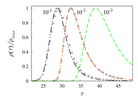
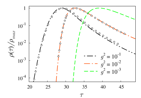
          (a)                                                                  (b)

Figure 5: (Color online) (a) Semiclassical (lines) and exact quantum–mechanical (points) traversal–time distributions in the model (7). The distributions are plotted in units of their maximal values $\rho_{max}$. Numbers near the graphs give values of $g^{2}$; the other parameters are $gp_{0}=1.52$, $g^{2}E_{y}=0.05$; $\sigma_{p}^{2}=0.005$, $gx_{2}=-gx_{1}=20$. (b) The same as (a) but in logarithmic scale.

In general case when the energy $E$ of the original unstable trajectory ${\bf x}(t)$ is substantially higher than $V_{0}$ the distribution $\rho(\tau)$ is not given by Eq. (28), regardless of whether $g^{2}$ is small or not. However, many qualitative features of $\rho_{u}(\tau)$ are valid in the higher–energy case as well. Consider e.g. Fig. 5a which corresponds to $(E-V_{0})/V_{0}\approx 0.2$. The distributions in this figure are highly asymmetric; they have long exponential tails at large $\tau$ and steep front–ends. Exponential behavior of $\rho(\tau)$ at large $\tau$ is illustrated in Fig. 5b where Fig. 5a is replotted in logarithmic scale. One writes,

$$\rho(\tau)\propto\exp(-\mbox{const}\cdot\tau)\;,$$ (32)

since the graphs in Fig. 5b are almost linear at $\tau\gg\langle\tau\rangle$.

In Figs. 5 we compare the semiclassical (lines) and exact quantum–mechanical (points) results for the traversal–time distributions; one observes agreement. The exact results are obtained by evolving numerically wave packets in full quantum system and implementing Eqs. (1), (2); we describe the respective numerical method in Appendix D.

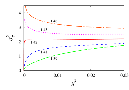
          (a)                                                                  (b)

Figure 6: (Color online) Mean times of passing (a) and time dispersions (b) as functions of $g^{2}$ in the model (7). Numbers near the graphs give values of $gp_{0}$. The other parameters are the same as in Figs. 5. Note that $gp_{c,1}\approx 1.421$; graphs with $p_{0}>p_{c,1}$ correspond to the case of sphaleron–driven tunneling.

The above properties of $\rho(\tau)$ naturally lead to large mean times of transmission $\langle\tau\rangle$ and large time dispersions $\sigma_{\tau}^{2}$ in the case of sphaleron–driven tunneling. In Figs. 6 we plot $\langle\tau\rangle$ and $\sigma_{\tau}^{2}$ as functions of $g^{2}$ at different values of $p_{0}$. One observes distinct behavior in the cases $p_{0}<p_{c,1}$ and $p_{0}>p_{c,1}$ corresponding to stable and unstable semiclassical dynamics, respectively. At small $p_{0}$ the graphs in Figs. 6 agree with Eqs. (20): $\langle\tau\rangle$ remains constant, and $\sigma_{p}^{2}$ vanishes in the limit $g^{2}\to 0$. In the unstable case $p_{0}>p_{c,1}$ one sees that $\langle\tau\rangle\sim|\log g^{2}|$ while $\sigma_{\tau}^{2}$ grows as $g^{2}\to 0$. Using these dependencies, one can discriminate between the standard and sphaleron–driven mechanisms of tunneling. Note that analogy with one–dimensional activation processes suggests logarithmic growth of $\langle\tau\rangle$ but constant $\sigma_{\tau}^{2}$, see Eqs. (29). Apparently, the unexpected behavior of $\sigma_{\tau}^{2}$ in Fig. 6b is related to features of non–linear multidimensional dynamics which deserve separate study.

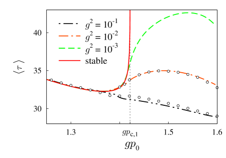
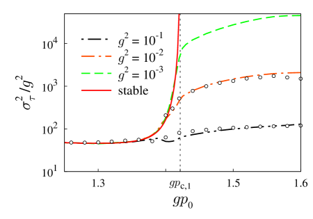
Figure 7: (Color online) Mean times of passing $\langle\tau\rangle$ and rescaled time dispersions $\sigma_{\tau}^{2}/g^{2}$ as functions of $gp_{0}$. The semiclassical and exact quantum–mechanical results are represented by lines and points, respectively. The parameters of the graphs are the same as in Figs. 5. The critical value $gp_{c,1}\approx 1.421$ is shown by the vertical dotted line.

In Figs. 7 we plot $\langle\tau\rangle$ and $\sigma_{\tau}^{2}/g^{2}$ as functions of mean initial momentum $p_{0}$. Dashed lines in these figures represent quantities computed with the distribution (17) at different values of $g^{2}$; they agree with the respective exact quantum–mechanical data (points). One sees that all graphs in Figs. 7 coincide in the region $p_{0}<p_{c,1}$ corresponding to stable trajectories. This is what one expects, since in stable case $\langle\tau\rangle$ and $\sigma_{\tau}^{2}/g^{2}$ are given by Eqs. (20) and therefore do not depend on $g^{2}$. “Stable” expressions (20) are represented by the solid lines. Above the critical momentum $p_{c,1}$ the situation in Figs. 7 changes drastically: both $\langle\tau\rangle$ and $\sigma_{\tau}^{2}/g^{2}$ depend on the semiclassical parameter, so that small $g^{2}$ correspond to large mean times of passing and large time dispersions.

Finally, let us repeat that the processes of sphaleron–driven tunneling survive in the limit $\sigma_{p}^{2}\to 0$, in contrast to one–dimensional activation processes of the previous Section. Our numerical calculations show that, indeed, at arbitrarily small $\sigma_{p}^{2}$ there exists a region of unstable semiclassical motions $p_{c,1}<p_{0}<p_{c,2}$; the width of this region stays finite in the limit $\sigma_{p}^{2}\to 0$.

5.3 Long–time behavior of traversal–time distribution

Let us return to the one–dimensional setup of Sec. 3 and consider transmission at high initial momentum $p_{0}>\sqrt{2V_{0}}$. This process is described by stable over–barrier trajectory $x(t)$ which passes the region $x_{1}<x<x_{2}$ in finite time $\tau=\langle\tau\rangle$. In the vicinity of $\langle\tau\rangle$ the distribution $\rho(\tau)$ is Gaussian, see Sec. 4. However, we are interested in the region $\tau\to+\infty$ where the value of $\rho(\tau)$ is exponentially small. We are going to show that in this region $\rho(\tau)$ does not resemble the Gaussian hat at all; rather, its form is similar to Eq. (28).

Semiclassically, the asymptotics of $\rho(\tau)$ is elucidated by studying the properties of the modified trajectories $x_{\epsilon}(\tau)$. At large $\tau$ these trajectories linger near the barrier top, see Eq. (26). One uses considerations of Sec. 5.1 and arrives at the formula

$$\rho_{a}(\tau)=\rho_{\infty}\cdot\mathrm{exp}\left\{-\omega_{-}\tau-\frac{2\epsilon_{0}}{g^{2}\omega_{-}}\,\mathrm{e}^{-\omega_{-}\tau}\right\}\;,$$ (33)

cf. Eq. (28). This asymptotics is universal, since parameters $\omega_{-}$, $\epsilon_{0}$ and $\rho_{\infty}$ disappear after appropriate shifts and rescalings of $\tau$ and $\rho$.

Let us point out one important difference between Eqs. (33) and (28). In Eq. (33) we consider the case of over–barrier transmissions when $\rho(\tau)$ reaches its maximum at finite $\tau=\langle\tau\rangle$. As one goes away from the maximum, the exponent $F_{\epsilon}$ in Eq. (17) grows. Since $\tau$–derivative of this exponent is equal to $-2\epsilon$, the parameter $\epsilon$ is negative at $\tau>\langle\tau\rangle$; thus, $\epsilon_{0}<0$ by Eq. (27). One concludes that the asymptotics (33) monotonically decreases with $\tau$ and $\rho_{\infty}$ is exponentially small.

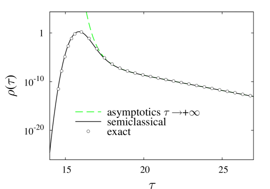
Figure 8: (Color online) Distribution $\rho(\tau)$ plotted for over–barrier transitions in the model (21); $g^{2}=0.002$, $p_{0}=1.45/g>\sqrt{2V_{0}}$, $\sigma_{p}^{2}=0.02$, $gx_{1}=-gx_{2}=10$.

In Fig. 8 we compare Eq. (33) (dashed line) with full semiclassical distribution (17) (solid line) and exact quantum mechanical results (points). One observes coincidence at $\tau\gg\langle\tau\rangle$.

6 Summary and remarks

The qualitative result of this paper is summarized as follows: quantum transitions take long times if they are described by unstable semiclassical trajectories. To understand how long this “long” is, we introduced the semiclassical parameter $g^{2}$ in Eq. (4). Then, unstable semiclassical dynamics can be identified in the limit $g^{2}\to 0$ where one obtains logarithmically large mean times of transitions and large time dispersions. This behavior is drastically different from that in the case of stable trajectories.

We defined traversal time from time–of–arrival measurements by the asymptotically distant detector. One may be unsatisfied with this definition and use another one, see e.g. Refs. [11, 12, 13, 14, 15]. However, the qualitative conclusion about large traversal times should be valid for any reasonable traversal–time definition, since large time delay comes from the almost–classical motion in the vicinity of the unstable mediator orbit (sphaleron or the barrier top).

The starting point of our analysis was general semiclassical expression (17) for the traversal–time distribution $\rho(\tau)$. In Sec. 5 we applied this expression to three processes related to unstable semiclassical dynamics: one–dimensional activation transitions, multidimensional processes of sphaleron–driven tunneling and over–barrier transmissions with large delays. The results were obtained analytically in one dimension, Eqs. (28) and (33), and numerically in the case of sphaleron–driven tunneling. We observed the following feature due to semiclassical instabilities: $\rho(\tau)$ is highly asymmetric and contains long exponential tail stretched toward $\tau\to+\infty$. This distribution is drastically different from Eq. (19) obtained in the case of stable trajectories.

Note that our results are somewhat different from those of Ref. [9] where power–law dependence of $|\Psi(\tau,x_{2})|^{2}$ on $\tau$ was reported. This dependence should be compared with the exponential tail of $\rho(\tau)$ in Fig. 5b. It seems that the difference can be explained in the following way. In the model of Ref. [9] many semiclassical trajectories contribute substantially into $\Psi(\tau,x_{2})$; one assumes that the number of these contributions grows with time $\tau$. On the other hand, only one trajectory is relevant in our model (7). Summation over large number of semiclassical contributions may be responsible for the modification of large–$\tau$ behavior of wave function in the model of Ref. [9] as compared to our case.

Unusual form of $\rho(\tau)$ and related scalings of $\langle\tau\rangle$, $\sigma_{\tau}^{2}$ with $g^{2}$ can be used for experimental identification of sphaleron–driven tunneling and one–dimensional activation transitions.

Acknowledgments.

We are indebted to S.V. Demidov, V.A. Rubakov and S.M. Sibiryakov for useful discussions and criticism. This work is supported in part by the grants of the President of Russian Federation NS-1616.2008.2, MK-1712.2008.2 (D.L.), Russian Science Support Foundation (A.P.), “Dynasty” Foundation (awarded by the Scientific board of ICPFM) and RFBR grant 08-02-00768-a. Numerical calculations were performed on the Computational cluster of Theoretical division of INR RAS.

Appendix A Semiclassical transmission probability

Let us evaluate semiclassically the total probability ${\cal P}_{\infty}$. For definiteness we consider two–dimensional model of Sec. 3; semiclassical calculations in one dimension are performed in the same way (see comments in Appendix C).

One starts with the path integral for the final state, Eq. (8). The in–state $\Psi_{i}$ entering this integral is described in Sec. 3. In the semiclassical approximation one writes,

$$\Psi_{i}({\bf x}_{i})=\frac{\sqrt{2\omega\sigma_{p}}}{(2\pi)^{3/4}\sqrt{p_{y}(y_{i})}}\cdot\mathrm{e}^{iB(x_{i},\,y_{i})+i\pi/4}\;,$$ (34)

where $p_{y}(y_{i})=\sqrt{2E_{y}-\omega^{2}y^{2}}$ is $y$–component of the initial momentum, and

$$B(x_{i},\,y_{i})=i\sigma_{p}^{2}(x_{i}-x_{1})^{2}+p_{0}x_{i}+\int_{\sqrt{2E_{y}}/\omega}^{y_{i}}p_{y}(y^{\prime})dy^{\prime}\;,$$ (35)

is in–state correction to the classical action.

Note that the integrand in Eq. (8) contains fast–oscillating exponent $\exp[i(S+B)]$, where $B$ comes from $\Psi_{i}$. Following the prescription of the saddle–point method, one finds the trajectory ${\bf x}(t)$ extremizing the functional $S+B$. In particular, ${\bf x}(t)$ should satisfy the classical equations of motion and Eqs. (9). After the saddle–point integration one obtains,

$$\Psi(\tau,{\bf x}_{f})=D_{1}^{-1/2}\cdot\mathrm{e}^{i(S+B)+i\pi/4}\;,$$ (36)

where all prefactors and saddle–point determinants are collected in $D_{1}$; we evaluate them below. We substitute Eq. (36) into the probability formula (1) and compute the saddle–point integral over ${\bf x}_{f}$. In this way we derive the conditions (10) and probability expression (11). [Note that $\tau$ is sent to infinity in the final formulas.] The suppression exponent of the probability is given by the value of the functional

$$F=2g^{2}\,\mathrm{Im}(S+B)$$ (37)

on the trajectory ${\bf x}(t)$. The probability prefactor

$$A=\frac{2\pi}{|D_{1}|\sqrt{D_{2}}}$$ (38)

involves additional determinant $D_{2}$ due to the saddle–point integration in Eq. (1).

Before proceeding with the factors $D_{1}$ and $D_{2}$, we preview the result for the probability prefactor $A$. One considers the set of perturbations $\delta{\bf x}(t)$ satisfying the linearized equations of motion

$$\delta\ddot{\bf x}+\hat{U}^{\prime\prime}({\bf x}(t))\delta{\bf x}=0$$ (39)

in the background of complex trajectory ${\bf x}(t)$. The basis in this set is formed by the “momentum” and “coordinate” perturbations $\boldsymbol{\psi}^{(j)}(t)$ and $\boldsymbol{\chi}^{(j)}(t)$, $j=1,2$. We assume that the basal perturbations satisfy two conditions: (i) they are normalized by

$$\Omega(\boldsymbol{\psi}^{(j)},\,\boldsymbol{\psi}^{(k)})=\Omega(\boldsymbol{\chi}^{(j)},\,\boldsymbol{\chi}^{(k)})=0\;,\qquad\qquad\Omega(\boldsymbol{\psi}^{(j)},\,\boldsymbol{\chi}^{(k)})=\delta^{jk}\;,$$

where $\Omega=d{\bf p}\wedge d{\bf x}$ is the canonical symplectic form; (ii) they are real in the out–region. Note that both of the above conditions can be imposed in the out–region and therefore constitute final Cauchy data for the perturbations $\boldsymbol{\psi}^{(j)}(t)$ and $\boldsymbol{\chi}^{(j)}(t)$. Note also that the basal perturbations are not completely specified by (i), (ii); in practice one fixes the freedom by supplying some additional data.

One introduces the functionals

$$\delta I_{1}[\delta{\bf x}]=\delta\dot{x}_{i}-2i\sigma_{p}^{2}\,\delta x_{i}\;,\qquad\qquad\delta I_{2}[\delta{\bf x}]=\dot{y}_{i}\delta\dot{y}_{i}+\omega^{2}y_{i}\delta y_{i}$$ (40)

which measure changes of initial conditions (9) caused by the perturbations $\delta{\bf x}(t)$. Changes due to the basal perturbations form two matrices,

$$\Pi_{jk}=\delta I_{j}[\boldsymbol{\psi}^{(k)}]\;,\qquad\qquad\Theta_{jk}=\delta I_{j}[\boldsymbol{\chi}^{(k)}]\;.$$ (41)

The probability prefactor is written in terms of these matrices,

$$A=\frac{2\omega\sigma_{p}}{\sqrt{2\pi\cdot\det[i\Theta\Pi^{+}-i\Pi\Theta^{+}]}}\;.$$ (42)

This expression is valid for any set of basal perturbations $\boldsymbol{\psi}^{(j)}$, $\boldsymbol{\chi}^{(j)}$ satisfying (i), (ii).

Semiclassical calculation of transmission probability ${\cal P}_{\infty}$ is summarized as follows. One finds the complex trajectory ${\bf x}(t)$ from the classical equations of motion and boundary conditions (9), (10). The exponent $F$ is given by the value of the functional (37) on this trajectory. One also constructs four linear perturbations $\boldsymbol{\psi}^{(j)}$, $\boldsymbol{\chi}^{(j)}$ by solving Eq. (39) with the Cauchy data (i), (ii) in the out–region. Prefactor $A$ is computed by Eq. (42); it involves changes of initial conditions due to the perturbations $\boldsymbol{\psi}^{(j)}$ and $\boldsymbol{\chi}^{(j)}$. Given $A$ and $F$, one finds the probability ${\cal P}_{\infty}$ from Eq. (11).

We derive Eq. (42) in two steps. First, we completely specify the basal perturbations $\boldsymbol{\psi}^{(j)}(t)$, $\boldsymbol{\chi}^{(j)}(t)$ and find $A$ in terms of these perturbations. Second, we prove that Eq. (42) is basis–independent once the conditions (i), (ii) are met.

One computes $D_{1}$ by collecting the prefactors in Eq. (8),

$$D_{1} =(2\pi)^{3/2}\frac{\dot{y}_{i}}{2\omega\sigma_{p}}\times(2\pi i)^{2}\left[\det\frac{\partial\dot{\bf x}_{f}}{\partial{\bf x}_{i}}\right]^{-1}\times\frac{1}{(2\pi i)^{2}}\det\frac{\partial^{2}(S+B)}{\partial{\bf x}_{i}^{2}}$$

$$=(2\pi)^{3/2}\frac{\dot{y}_{i}}{2\omega\sigma_{p}}\det\frac{\partial^{2}(S+B)}{{\partial\dot{\bf x}_{f}}\partial{\bf x}_{i}}\;,$$ (43)

where ${\bf x}_{f}$ is kept constant in the differentiations. Three factors in the first line come from the initial state (34) and saddle–point integrals over ${\bf x}(t)$ and ${\bf x}_{i}$, respectively. Evaluating explicitly the derivatives of $S$ and $B$, one obtains,

$$D_{1}=\frac{(2\pi)^{3/2}}{2\omega\sigma_{p}}\det\left[\begin{pmatrix}1&0\\ 0&\dot{y}_{i}\end{pmatrix}\frac{\partial\dot{\bf x}_{i}}{\partial\dot{\bf x}_{f}}+\begin{pmatrix}-2i\sigma_{p}^{2}&0\\ 0&\omega^{2}y_{i}\end{pmatrix}\frac{\partial{\bf x}_{i}}{\partial\dot{\bf x}_{f}}\right]\Bigg{|}_{{\bf x}_{f}=\mathrm{const}}\;,$$ (44)

where we wrote $\dot{y}_{i}$ as a determinant of diagonal matrix and performed matrix multiplication. We choose the basal perturbations $\boldsymbol{\psi}^{(1)}(t)=\partial{\bf x}(t)/\partial\dot{x}_{f}$, $\boldsymbol{\psi}^{(2)}(t)=\partial{\bf x}(t)/\partial\dot{y}_{f}$, where the derivatives are taken at fixed ${\bf x}_{f}$. Clearly, these perturbations satisfy the linearized equations (39). Their final Cauchy data are

$$\boldsymbol{\psi}^{(1)}(\tau)=\boldsymbol{\psi}^{(2)}(\tau)=0\;,\qquad\qquad\boldsymbol{\dot{\psi}}^{(1)}(\tau)=\begin{pmatrix}1\\ 0\end{pmatrix}\;,\qquad\qquad\boldsymbol{\dot{\psi}}^{(2)}(\tau)=\begin{pmatrix}0\\ 1\end{pmatrix}\;.$$ (45)

In terms of $\boldsymbol{\psi}$–perturbations

$$D_{1}=\frac{(2\pi)^{3/2}}{2\omega\sigma_{p}}\cdot\det\Pi\;,$$

where $\Pi$ is $2\times 2$ matrix defined in Eq. (41).

Determinant $D_{2}$ comes from the integration in Eq. (1),

$$D_{2}=\det\left[-i\frac{\partial\dot{\bf x}_{f}}{\partial{\bf x}_{f}}+\mathrm{h.c}\right]\;,$$ (46)

where the derivatives are taken in the subclass of trajectories satisfying Eqs. (9). Let us define two remaining basal perturbations as $\boldsymbol{\chi}^{(1)}(t)=\partial{\bf x}(t)/\partial x_{f}$, $\boldsymbol{\chi}^{(2)}(t)=\partial{\bf x}(t)/\partial y_{f}$, where $\dot{\bf x}_{f}$ is kept fixed in the differentiations. These perturbations satisfy

$$\boldsymbol{\chi}^{(1)}(\tau)=\begin{pmatrix}1\\ 0\end{pmatrix}\;,\qquad\qquad\boldsymbol{\chi}^{(2)}(\tau)=\begin{pmatrix}0\\ 1\end{pmatrix}\;,\qquad\qquad\boldsymbol{\dot{\chi}}^{(1)}(\tau)=\boldsymbol{\dot{\chi}}^{(2)}(\tau)=0\;.$$ (47)

Note that the matrix in $D_{2}$ is not directly related to $\boldsymbol{\chi}$–perturbations, since the differentiations in Eq. (46) are performed with Eqs. (9) kept fixed. One introduces two auxiliary perturbations

$$\boldsymbol{\kappa}^{(1)}(t)=\frac{\partial{\bf x}(t)}{\partial x_{f}}\Bigg{|}_{\mathrm{Eqs.~{}(\ref{eq:18})}}\;,\qquad\qquad\boldsymbol{\kappa}^{(2)}(t)=\frac{\partial{\bf x}(t)}{\partial y_{f}}\Bigg{|}_{\mathrm{Eqs.~{}(\ref{eq:18})}}$$ (48)

which enter Eq. (46). They can be decomposed in the $\boldsymbol{\psi}$, $\boldsymbol{\chi}$–basis,

$$\boldsymbol{\kappa}^{(j)}=\sum_{k=1}^{2}A_{jk}\,\boldsymbol{\psi}^{(k)}+\boldsymbol{\chi}^{(j)}\;,$$ (49)

where we took into account Eqs. (45), (47). Since $\boldsymbol{\kappa}$–perturbations do not change the initial conditions, one writes $\delta I_{j}[\boldsymbol{\kappa}^{(k)}]=0$. Substituting representation (49) into these equations, one obtains

$$A^{T}=-\Pi^{-1}\Theta\;.$$

We finally write $D_{2}$ in terms of the perturbations $\boldsymbol{\kappa}^{(j)}$ and use Eq. (49). We find,

$$D_{2}=|\det\Pi|^{-2}\cdot\det[i\Theta\Pi^{+}-i\Pi\Theta^{+}]\;.$$

Using expressions for $D_{1}$, $D_{2}$ and Eq. (38), one gets Eq. (42).

We finish this Appendix by proving that any set of basal perturbations with properties (i), (ii) can be used in Eq. (42). Note first that $\boldsymbol{\psi}^{(j)}$, $\boldsymbol{\chi}^{(j)}$ introduced in Eqs. (45), (47) do satisfy these properties. Denote by ${\boldsymbol{\tilde{\psi}}}^{(i)}$, ${\boldsymbol{\tilde{\chi}}}^{(i)}$ some other set which also passes (i), (ii). One decomposes new perturbations in the old basis, substitutes them into Eq. (42) and uses (i), (ii). In this way one proves that the value of the prefactor (42) does not depend on the choice for basal perturbations once they are real in the out–region and correctly normalized.

Appendix B Expression for $\rho(\tau)$

Here we give details of the semiclassical evaluation of $\rho(\tau)$ which was outlined in Sec. 4. We start by computing the integral in brackets in Eq. (14). The result is (cf. Eq. (36))

$$\Psi(\tau,{\bf x}_{f})=\int_{0}^{\tau}d\tau^{\prime}\int_{i\infty}^{-i\infty}\frac{id\epsilon}{2\pi g^{2}}\;D_{1,\epsilon}^{-1/2}\cdot\mathrm{e}^{i(S_{\epsilon}[{\bf x}_{\epsilon}]+B[{\bf x}_{\epsilon}])+i\pi/4}\;,$$ (50)

where $S_{\epsilon}=S+i\epsilon(T_{int}-\tau^{\prime})/g^{2}$ is the modified action. By subscripts $\epsilon$ here we mark the quantities computed with the modified trajectory ${\bf x}_{\epsilon}(t)$ and modified action $S_{\epsilon}$. Recall that ${\bf x}_{\epsilon}(t)$ extremizes $S_{\epsilon}$, arrives at ${\bf x}_{\epsilon}(\tau)={\bf x}_{f}$ and satisfies the initial conditions (9).

Now, we evaluate the integral over $\epsilon$ in Eq. (50). Since ${\bf x}_{\epsilon}(t)$ extremizes $S_{\epsilon}+B$, one writes,

$$\frac{d}{d\epsilon}(S_{\epsilon}+B)=\frac{d{\bf x}_{\epsilon}}{d\epsilon}\cdot\frac{\delta}{\delta{\bf x}_{\epsilon}}(S_{\epsilon}+B)+\frac{\partial}{\partial\epsilon}(S_{\epsilon}+B)=i(T_{int}-\tau^{\prime})/g^{2}\;.$$ (51)

Thus, the exponent in Eq. (50) is extremal with respect to $\epsilon$ when $T_{int}[{\bf x}_{\epsilon}]=\tau^{\prime}$. Performing the saddle–point integration over $\epsilon$, one obtains,

$$\Psi(\tau,{\bf x}_{f})=\int_{0}^{\tau}\frac{d\tau^{\prime}}{g\sqrt{2\pi D_{1,\epsilon}}}\sqrt{-\frac{d\epsilon}{d\tau^{\prime}}}\cdot\mathrm{e}^{i(S_{\epsilon}+B)+i\pi/4}\;.$$ (52)

Additional prefactor in this expression arises due to fixation of $T_{int}$.

Next, we substitute $\Psi_{f}$ into the probability formula (1). Note that ${\cal P}_{\tau}$ involves, besides $\Psi(\tau,{\bf x}_{f})$, its complex conjugate. Starting with the path integral for the latter, one shows that expression for $\Psi^{*}(\tau,{\bf x}_{f})$ is obtained from Eq. (52) by changing the signs of the exponent and $\epsilon$. We write,

$${\cal P}_{\tau}=\int d{\bf x}_{f}\int_{0}^{\tau}\frac{d\tau^{\prime}d\bar{\tau}}{2\pi g^{2}\sqrt{D_{1,\epsilon}D_{1,-\bar{\epsilon}}}}\sqrt{\frac{d\epsilon}{d\tau^{\prime}}\frac{d\bar{\epsilon}}{d\bar{\tau}}}\cdot\mathrm{e}^{i(S_{\epsilon}[{\bf x}_{\epsilon}]+B[{\bf x}_{\epsilon}])-i(S_{-\bar{\epsilon}}[{\bf x}_{-\bar{\epsilon}}]+B[{\bf x}_{-\bar{\epsilon}}])}\;,$$ (53)

where $\bar{\tau}$ and $\bar{\epsilon}$ come from $\Psi^{*}(\tau,{\bf x}_{f})$; they are related by $T_{int}[{\bf x}_{-\bar{\epsilon}}]=\bar{\tau}$.

One sees that the probability formula involves integrals over two traversal times $\tau^{\prime}$ and $\bar{\tau}$ spent by the respective trajectories in the region $x<x_{2}$. We introduce new variables $\tau_{+}=(\tau^{\prime}+\bar{\tau})/2$ and $\tau_{-}=\tau^{\prime}-\bar{\tau}$ and perform the integral over $\tau_{-}$ in the saddle–point approximation. This leads to the condition $\epsilon=\bar{\epsilon}$. Note that after the integration the value of $\epsilon$ is related to $\tau_{+}$ by the implicit relation

$$T_{int}[{\bf x}_{\epsilon}]+T_{int}[{\bf x}_{-\epsilon}]=2\tau_{+}\;.$$ (54)

Assuming that the trajectory ${\bf x}_{\epsilon}(t)$ is unique, one proves that the saddle–point value of $\epsilon$ is real. Indeed, it is straightforward to check that ${\bf x}_{\epsilon}^{*}={\bf x}_{-\epsilon^{*}}$. Thus, for real $\epsilon$ the function $\tau_{+}(\epsilon)$ is real, see Eq. (54). The same is correct for the inverse function $\epsilon(\tau_{+})$. Equation (54) and reality of $\epsilon$ lead to the relation

$$\mathrm{Re}\,T_{int}[{\bf x}_{\epsilon}]=\tau_{+}$$ (55)

which implies that $\tau_{+}$ is the real part of the time interval spent by the modified trajectory in the region between $x_{1}$ and $x_{2}$.

Finally, let us evaluate the integral over ${\bf x}_{f}$ in Eq. (53). It is taken in the same way as in Appendix A. However, we obtain conditions at finite $\tau$,

$$\mathrm{Im}\,\dot{\bf x}_{\epsilon}(\tau)=\mathrm{Im}\,{\bf x}_{\epsilon}(\tau)=0$$ (56)

cf. Eqs. (10).

We arrive at the following representation,

$${\cal P}_{\tau}=\int_{0}^{\tau}\frac{d\tau_{+}}{\sqrt{\pi g^{2}}}\left[-\frac{d\epsilon}{d{\tau_{+}}}\right]^{1/2}A_{\epsilon}\cdot\mathrm{e}^{-F_{\epsilon}/g^{2}}\;,$$ (57)

where only the integral over $\tau_{+}$ is left. Quantities $F_{\epsilon}$ and $A_{\epsilon}$ in this formula are given by the same expressions (37) and (42), but with the modified action (15) and modified trajectory ${\bf x}_{\epsilon}(t)$. Note that now $\tau_{+}$ enters the modified action $S_{\epsilon}$ instead of $\tau^{\prime}$.

In Refs. [26] representation similar to Eq. (57) was used for evaluation of total transmission probability ${\cal P}_{\infty}$. In this case one sends $\tau$ to infinity and performs the integral over $\tau_{+}$. We follow another path and calculate $\rho(\tau)$ by differentiating Eq. (57) with respect to $\tau$.

Let us show that the integrand in Eq. (57) does not depend on the duration of the process $\tau$. Consider first the modified trajectory ${\bf x}_{\epsilon}(t)$. Parameter $\tau$ enters the boundary value problem for ${\bf x}_{\epsilon}(t)$ via the conditions (56) imposed at $t=\tau$. Note, however, that ${\bf x}_{\epsilon}(\tau)$ lies inside the detection region $x>x_{2}$. Indeed, due to Eq. (55) $\tau_{+}$ is equal to the time of motion in the region $x<x_{2}$; at $\tau_{+}<\tau$ the trajectory leaves this region before $t=\tau$. From Eqs. (15), (12) one finds that the classical equations of motion are not modified in the detection region $x>x_{2}$. Thus, ${\bf x}_{\epsilon}(t)$ describes real classical evolution at $t\approx\tau$, and conditions of reality, Eqs. (56), can be imposed at any point of this evolution without affecting the trajectory. One concludes that ${\bf x}_{\epsilon}(t)$ does not depend on $\tau$. The suppression exponent $F_{\epsilon}$, Eq. (37), is independent of $\tau$ as well, since it involves the imaginary part of $S_{\epsilon}$ computed on the modified trajectory. Function $\epsilon(\tau_{+})$ is defined in Eq. (55); it does not depend on $\tau$ due to definition of $T_{int}$, see Eq. (12).

Now, we change the duration of the process, $\tau\to\tau+\delta\tau$, and find the respective changes of the basal perturbations $\boldsymbol{\psi}$, $\boldsymbol{\chi}$. For concreteness we use the perturbations defined by Eqs. (45), (47). Solving explicitly Eqs. (39) in the asymptotic region $x>x_{2}$, we find that

$$\begin{pmatrix}\boldsymbol{\psi}^{(1)}\\ \boldsymbol{\chi}^{(1)}\end{pmatrix}\to\begin{pmatrix}1&-\delta\tau\\ 0&1\end{pmatrix}\begin{pmatrix}\boldsymbol{\psi}^{(1)}\\ \boldsymbol{\chi}^{(1)}\end{pmatrix}\;,\qquad\begin{pmatrix}\boldsymbol{\psi}^{(2)}\\ \boldsymbol{\chi}^{(2)}\end{pmatrix}\to\begin{pmatrix}\cos(\omega\delta\tau)&-\sin(\omega\delta\tau)/\omega\\ \omega\sin(\omega\delta\tau)&\cos(\omega\delta\tau)\end{pmatrix}\begin{pmatrix}\boldsymbol{\psi}^{(2)}\\ \boldsymbol{\chi}^{(2)}\end{pmatrix}\;,$$ (58)

due to $\delta\tau$. Using these transformations, one explicitly proves that $A_{\epsilon}$, Eq. (42), does not depend on $\tau$.

Now, take a look at the probability ${\cal P}_{\tau}$, Eq. (57). We have shown that the quantities $F_{\epsilon}$, $\epsilon(\tau_{+})$, $A_{\epsilon}$ in the integrand of this expression do not depend on $\tau$. Thus, the derivative $\rho(\tau)$, Eq. (2), is simply given by the integrand at $\tau_{+}=\tau$. In this way one gets the semiclassical expression (17) of Sec. 4; the relation (16) is obtained from Eq. (55).

Finally, we prove Eq. (18):

$$\frac{dF_{\epsilon}}{d\tau}=\frac{\partial F_{\epsilon}}{\partial\tau}=-2\epsilon\;,$$ (59)

since $F_{\epsilon}$ is extremal with respect to ${\bf x}_{\epsilon}(t)$ and $\epsilon$.

Appendix C Semiclassical calculations in one dimension

In this Appendix we perform explicit semiclassical calculations in the model (21).

For a start, we find the original complex trajectory $x(t)$. General classical solution with energy $E<V_{0}\equiv 1/g^{2}$ looks like

$$\sqrt{\frac{g^{2}E}{1-g^{2}E}}\cdot\mathrm{sh}(gx)=\mathrm{ch}\,\left[g\sqrt{2E}(t-t_{0})\right]\;,$$ (60)

where $E$ and $t_{0}$ are real by Eqs. (10). One notes that the solution (60), if taken along the real time axis, describes reflection from the potential barrier; trajectory with correct asymptotics is obtained by winding the time contour around the nearest upper branching point of the solution. From the initial condition (9) one finds the energy of the solution, $E=(p_{0}+2\pi\sigma_{p}^{2}/g)^{2}/2$. Since $E$ does not exceed the height of the potential barrier, the value of $p_{0}$ is smaller than $p_{c,1}$, Eq. (24).

The case $E>V_{0}$ corresponds to classical over–barrier motions which trivially produce $E=p_{0}^{2}/2$ and therefore $p_{0}>\sqrt{2V_{0}}=p_{c,2}$. One concludes that transitions in the region $p_{c,1}<p_{0}<p_{c,2}$ are not described by the trajectories with $E\neq V_{0}$. The remaining solution

$$\mathrm{sh}(gx)=-\mathrm{exp}\left[-\sqrt{2}(t-t_{0})\right]$$ (61)

corresponds to $E=V_{0}=1/g^{2}$. It starts in the in–region and approaches the barrier top as $t\to+\infty$. Note that Eq. (61) automatically passes the final boundary conditions (10). Thus, $t_{0}$ is complex; one finds it from Eq. (9). Trajectories (61) exist at any $p_{0}$. Calculating the suppression exponent (37), one explicitly checks that they are sub–dominant outside the interval $p_{c,1}<p_{0}<p_{c,2}$ and describe transitions through the barrier if $p_{0}$ belongs to this interval.

Note that the fixed–energy transmission coefficients ${\cal P}_{p}$ are exactly known in the model (21). Using these coefficients and Eq. (22), one explicitly confirms the semiclassical expressions for ${\cal P}_{\infty}$, Refs. [26], in cases of stable and unstable semiclassical dynamics.

We proceed by introducing modification. One notices that the modified potential (25) involves step–function and therefore has two analytic continuations, which start from the regions $x<x_{2}$ and $x>x_{2}$. We find the corresponding parts of the modified trajectory and sew them and their time derivatives at $t=t_{2}$ where $x_{\epsilon}(t_{2})=x_{2}$. Note that the energy $E$ of trajectory is conserved across the sewing point. The time $t_{2}$ and energy $E$ are real due to the final boundary conditions (10). Moreover, $t_{2}=\tau$ by Eq. (16). At $t<t_{2}$ the modification adds the imaginary constant $-i\epsilon/g^{2}$ to the potential. Thus, in this region $x_{\epsilon}(t)$ is given by Eq. (60) where one should substitute $E\to E_{\epsilon}=E+i\epsilon/g^{2}$. Note that parameter $t_{0}$ is complex after modification: it is found from $x_{\epsilon}(\tau)=x_{2}$. Using this condition and Eq. (9), one obtains non–linear complex equation

$$f(E_{\epsilon})\equiv\frac{i}{2\sigma_{p}^{2}}\left(\sqrt{2E_{\epsilon}}-p_{0}\right)+x_{2}-x_{1}-\sqrt{2E_{\epsilon}}\,\tau+\frac{1}{g}\cdot\mathrm{ln}\,\frac{g^{2}E_{\epsilon}}{g^{2}E_{\epsilon}-1}=0$$ (62)

which relates $E$ and $\epsilon$ to $p_{0}$ and $\tau$.

Now, we compute $\rho(\tau)$ using the modified quantities $\epsilon$, $F_{\epsilon}$, $A_{\epsilon}$ and Eq. (17). The function $\epsilon(\tau)$ is found from Eq. (62). The modified exponent $F_{\epsilon}$ is computed by substituting $S_{\epsilon}$ and $x_{\epsilon}(t)$ into Eq. (37) and performing integration. [We disregard the $y$–dependent part of the functional $B$, Eq. (35).] The final ingredient is the probability prefactor $A_{\epsilon}$ which is given by one–dimensional formula

$$A=\frac{\sigma_{p}\sqrt{2}}{\sqrt{\mathrm{Im}(\delta I_{1}^{*}[\chi]\cdot\delta I_{1}[\psi])}}\;.$$ (63)

Here by omitting the subscript $\epsilon$ we mean that Eq. (63) can be used both in modified and unmodified cases. Note that one–dimensional prefactor can be obtained from Eq. (42) by reducing the size of matrices $\Pi$ and $\Theta$ and omitting the kinematical factor $\omega/\sqrt{2\pi}$.

Linear perturbations $\chi_{\epsilon}$, $\psi_{\epsilon}$ are calculated by differentiating the trajectory $x_{\epsilon}(t)$ with respect to parameters,

$$\chi_{\epsilon}(t)=\frac{\dot{x}_{\epsilon}(t)}{\sqrt{2E}}\;,\qquad\qquad\psi_{\epsilon}(t)=\alpha\dot{x}_{\epsilon}(t)+\beta\frac{\partial x_{\epsilon}(t)}{\partial p_{0}}\;,$$

where we have already used the Cauchy data (47) for $\chi(t)$. Conditions (45) give $\beta^{-1}=\partial\sqrt{2E}/\partial p_{0}$, where the derivative is taken at $\epsilon=\mathrm{const}$. Substituting the perturbations into Eq. (63), and using Eq. (9), one arrives at the expression

$$A_{\epsilon}=\left(\frac{\partial E}{\partial p_{0}}\Big{/}\mathrm{Re}\,\sqrt{2E_{\epsilon}}\right)^{1/2}$$

for the probability prefactor.

We substitute $F_{\epsilon}$ and $A_{\epsilon}$ into Eq. (17) and use some algebra. The result is

$$\rho(\tau)={\cal N}^{\prime}\cdot\left|\frac{df(E_{\epsilon})}{dE_{\epsilon}}\right|^{-1}\cdot\mathrm{exp}\left\{-\frac{1}{\sigma_{p}^{2}}\left(p_{0}^{2}/2-E\right)-\frac{2\epsilon\tau}{g^{2}}+\frac{2\sqrt{2}}{g^{2}}\mathrm{arg}\left(\frac{\sqrt{E_{\epsilon}}+1/g}{\sqrt{E_{\epsilon}}-1/g}\right)\right\}\;,$$ (64)

where ${\cal N}^{\prime}$ is normalization factor. Note that $f(E_{\epsilon})$ is defined in Eq. (62), and the values of $E$, $\epsilon$ are found from $f(E_{\epsilon})=0$.

The expectation value $\langle\tau\rangle$ of the distribution (64) is plotted in Fig. 3b, solid line. “Stable” and “unstable” distributions, Eqs. (19) and (28), (30) are obtained by considering Eqs. (62), (64) in the region of small $\epsilon$.

Appendix D Exact results in two dimensions

We compute exact traversal–time distributions in the model (7) using the following numerical procedure.

First of all, we introduce the basis of stationary eigenfunctions $\psi_{p}(x,y)$ satisfying time–independent Schrödinger equation with scattering boundary conditions,

$$\begin{array}[]{ll}\psi_{p}(x,y)\to\psi_{y}(y)\cdot\mathrm{e}^{ipx}+\mbox{reflected waves}\;,&\mbox{as}\qquad x\to-\infty\;,\\ \psi_{p}(x,y)\to\mbox{outgoing waves}\;,&\mbox{as}\qquad x\to+\infty\;,\end{array}$$ (65)

where $\psi_{y}(y)$ is the initial oscillator state with energy $E_{y}$. The total energy corresponding to $\psi_{p}(x,y)$ is $E_{p}=p^{2}/2+E_{y}$.

One decomposes the initial wave packet $\Psi_{i}$ (Sec. 3) in the above basis,

$$\Psi_{i}(x,y)=\psi_{x}(x)\cdot\psi_{y}(y)=\frac{1}{\sqrt{2\pi}}\int dp\;\psi_{x}(p)\,\mathrm{e}^{ipx}\cdot\psi_{y}(y)=\frac{1}{\sqrt{2\pi}}\int dp\;\psi_{x}(p)\,\psi_{p}(x,y)\;,$$

where we performed Fourier transformation and used the asymptotics (65) of $\psi_{p}(x,y)$. Then, we propagate the wave packet from $t=0$ to $t=\tau$,

$$\Psi(\tau,\,x,y)=\frac{1}{\sqrt{2\pi}}\int dp\;\psi_{x}(p)\,\psi_{p}(x,y)\cdot\mathrm{e}^{-iE_{p}\tau}\;.$$ (66)

Given representation (66) one computes the total probability current through the line $x=x_{2}$. The distribution $\rho(\tau)$ is proportional to this current, see Sec. 2; the proportionality coefficient is obtained from the normalization condition $\int\rho(\tau)\,d\tau=1$.

In practice we computed the exact distributions $\rho(\tau)$ at $g^{2}=0.1$ and $0.01$. At each value of $g^{2}$ we generated the set of eigenfunctions $\psi_{p}(x,y)$ by solving numerically the stationary Schrödinger equation at several energies $E_{p}$. To this end we used the numerical method of Ref. [33] (see Ref. [38] for the Fortran 90 code). Given the eigenfunctions, we constructed the linear combination (66) and calculated the total probability current through the line $x=x_{2}$. Computing numerically the normalization integral, we finally obtained $\rho(\tau)$.

There are two limitations of our numerical procedure; both of them are relevant for the numerical data at $g^{2}=0.01$. First, our method of solving the Schrödinger equation fails to produce correct eigenfunctions at $g^{2}=0.01$ and $E_{p}<1$. Accordingly, the exact data at $g^{2}=0.01$ in Figs. 7 are limited to the region $gp_{0}\geq 1.4$ where the contributions of low–energy eigenfunctions are negligible. Second, due to cancellations in the integral (66) we are not able to compute directly the probability current at large $\tau$ (see, e.g., Figs. 5 where the exact distributions are obtained at $\tau\lesssim 45$). This prevents us from normalizing directly the $g^{2}=0.01$ distributions which fall off slowly at large $\tau$. Due to this feature we consider the normalization–independent quantity $\rho(\tau)/\rho_{\max}$ in Figs. 5. The exact data at $g^{2}=0.01$ in Figs. 6 are obtained by extrapolating the corresponding distributions with the conjectured behavior (32). After extrapolation we normalize the distributions and compute the values of $\langle\tau\rangle$ and $\sigma_{\tau}^{2}$.

We stress that the limitations listed above are not present at $g^{2}=0.1$; in this case the exact distributions $\rho(\tau)$ can be computed directly at all values of $gp_{0}$.

References

- [1] S. C. Creagh, in Tunneling in complex systems, ed. by S. Tomsovic (World Scientific, Singapore, 1998). S. Tomsovic, Phys. Scr. T90, 162 (2001).
- [2] W. H. Miller, Adv. Chem. Phys. 25, 69 (1974).
- [3] S. Takada and H. Nakamura, J. Chem. Phys. 100, 98 (1994).
- [4] W. H. Miller, J. Chem. Phys. 48, 1651 (1968). R. E. Meyer, SIAM J. Appl. Math. 51, 1585 (1991); ibid. 51, 1602 (1991). S. C. Creagh, J. Phys. A 27, 4969 (1994).
- [5] M. Wilkinson, Physica D 21, 341 (1986); J. Phys. A 20, 635 (1987). S. Takada, P. N. Walker and M. Wilkinson, Phys. Rev. A 52, 3546 (1995). S. Takada, J. Chem. Phys. 104, 3742 (1996). S. C. Creagh and M. D. Finn, J. Phys. A 34, 3791 (2001). G. C. Smith and S. C. Creagh, J. Phys. A 39, 8283 (2006).
- [6] O. Bohigas, S. Tomsovic and D. Ullmo, Phys. Rep. 223, 43 (1993). E. Doron and S. D. Frischat, Phys. Rev. Lett. 75, 3661 (1995). S. D. Frischat and E. Doron, Phys. Rev. E 57, 1421 (1998). A. Shudo and K. S. Ikeda, Phys. Rev. Lett. 74, 682 (1995); Physica D 115, 234 (1998). A. Mouchet, C. Miniatura, R. Kaiser, B. Grémaud and D. Delande, Phys. Rev. E 64, 016221 (2001). A. D. Ribeiro, M. A. M. de Aguiar and M. Baranger, Phys. Rev. E 69, 066204 (2004). D. G. Levkov, A. G. Panin and S. M. Sibiryakov, Phys. Rev. E 76 046209 (2007). A. Bäcker, R. Ketzmerick, S. Löck and L. Schilling, Phys. Rev. Lett. 100, 104101 (2008).
- [7] M. Wilkinson, J. H. Hannay, Physica D 27, 201 (1987). S. C. Creagh and N. D. Whelan, Phys. Rev. Lett. 77, 4975 (1996); ibid. 82, 5237 (1999).
- [8] C. Dembowski et al, Phys. Rev. Lett. 84, 867 (2000); R. Hofferbert et al, Phys. Rev. E 71, 046201 (2005). W. K. Hensinger et al, Nature 412, 52 (2001); W. K. Hensinger et al, Phys. Rev. A 70, 013408 (2004). D. A. Steck, W. H. Oskay and M. G. Raizen, Science 293, 274 (2001); Phys. Rev. Lett. 88, 120406 (2002). A. Bäcker et al, Phys. Rev. Lett. 100, 174103 (2008).
- [9] K. Takahashi and K. S. Ikeda, Phys. Rev. Lett. 97, 240403 (2006).
- [10] E. H. Hauge, G. A. Støvneng, Rev. Mod. Phys. 61, 917 (1989). R. Landauer, Th. Martin, Rev. Mod. Phys. 66, 217 (1994). Time in Quantum Mechanics, ed. by J. G. Muga, R. Sala Mayato, Í. L. Egusquiza (Springer, Berlin/Heidelberg, 2008).
- [11] D. Bohm, Quantum Theory (Prentice-Hall, New York, 1951). E. P. Wigner, Phys. Rev. 98, 145 (1955).
- [12] F. T. Smith, Phys. Rev. 118, 349 (1960).
- [13] A. I. Baz’, Sov. J. Nucl. Phys. 4, 182 (1967). V. F. Rubachenko, Sov. J. Nucl. Phys. 5, 635. (1967). M. Büttiker, Phys. Rev. B 27, 6178 (1983).
- [14] M. Büttiker, R. Landauer, Phys. Rev. Lett. 49, 1739 (1982).
- [15] D. Sokolovski, L. M. Baskin, Phys. Rev. A 36, 4604 (1987). D. Sokolovski, in Time in Quantum Mechanics, ed. by J. G. Muga, R. Sala Mayato, Í. L. Egusquiza (Springer, Berlin/Heidelberg, 2008).
- [16] T. Ohmura, Prog. Theor. Phys. Suppl. 29, 108 (1964).
- [17] W. Jaworski, D. M. Wardlaw, Phys. Rev. A 37, 2843 (1988).
- [18] V. S. Olkhovsky and E. Recami, Phys. Rep. 214, 339 (1992); V. S. Olkhovsky, E. Recami, F. Raciti and A. K. Zaichenko, J. Phys. I France 5, 1351 (1995). G. Privitera, G. Salesi, V. S. Olkhovsky and E. Recami, Riv. Nuovo Cim. 26, n. 4, 1 (2003).
- [19] C. Anastopoulos, N. Savvidou, J. Math. Phys. 47, 122106 (2006); ibid. 49, 022101 (2008).
- [20] F. Bezrukov and D. Levkov, arXiv:quant-ph/0301022; J. Exp. Theor. Phys. 98, 820 (2004) [Zh. Eksp. Teor. Fiz. 125, 938 (2004)].
- [21] K. Takahashi and K.S. Ikeda, J. Phys. A 36, 7953 (2003); Europhys. Lett. 71, 193 (2005); erratum-ibid 75, 355 (2006).
- [22] T. Onishi, A. Shudo, K. S. Ikeda, and K. Takahashi, Phys. Rev. E 64, 025201(R) (2001); ibid 68, 056211 (2003).
- [23] F. R. Klinkhamer and N. S. Manton, Phys. Rev. D 30, 2212 (1984).
- [24] S. Wiggins, L. Wiesenfeld, C. Jaffé and T. Uzer, Phys. Rev. Lett. 86, 5478 (2001).
- [25] F. Bezrukov, D. Levkov, C. Rebbi, V. Rubakov and P. Tinyakov, Phys. Rev. D 68, 036005 (2003); Phys. Lett. B 574, 75 (2003). D. G. Levkov and S. M. Sibiryakov, Phys. Rev. D 71, 025001 (2005); JETP Lett. 81, 53 (2005) [Pisma Zh. Eksp. Teor. Fiz. 81, 60 (2005)].
- [26] D. G. Levkov, A. G. Panin and S. M. Sibiryakov, Phys. Rev. Lett. 99, 170407 (2007); J. Phys. A: Math. Theor. 42, 205102 (2009).
- [27] K. Takahashi and K. S. Ikeda, J. Phys. A 41, 095101 (2008); Phys. Rev. A 79, 052114 (2009). A. Shudo, Y. Ishii and K. S. Ikeda, Europhys. Lett. 81, 50003 (2008).
- [28] E. H. Hauge, J. P. Falck, T. A. Fjeldly, Phys. Rev. B 36, 4203 (1987). C. R. Leavens, G. C. Aers, Phys. Rev. B 39, 1202 (1989).
- [29] A. M. Steinberg, P. G. Kwiat, and R. Y. Chiao, Phys. Rev. Lett. 71, 708 (1993).
- [30] H. G. Winful, Phys. Rep. 436, 1 (2006). A. M. Steinberg, in Time in Quantum Mechanics, ed. by J. G. Muga, R. Sala Mayato, Í. L. Egusquiza (Springer, Berlin/Heidelberg, 2008).
- [31] T. E. Hartman, J. Appl. Phys. 33, 3427 (1962).
- [32] Y. Japha, G Kurizki, Phys. Rev. A 53, 586 (1996).
- [33] G. F. Bonini, A. G. Cohen, C. Rebbi and V. A. Rubakov, Phys. Rev. D 60, 076004 (1999); quant-ph/9901062.
- [34] M. J. Davis and E. J. Heller, J. Chem. Phys. 75, 246 (1981); E. J. Heller and M. J. Davis, J. Phys. Chem. 85, 307 (1981).
- [35] E. J. Gumbel, Statistics of extremes, Columbia University Press, New York, 1958.
- [36] Claudio Rebbi, lecture notes and software for the course PY421, http://physics.bu.edu/~rebbi
- [37] J. H. Van Vleck, Proc. Natl. Acad. Sci. USA 14, 178 (1928). H. Kleinert, Path Integrals in Quantum Mechanics, Statistics, Polymer Physics, and Financial Markets, World Scientific, Singapore, 2006.
- [38] http://solver.inr.ac.ru