Theory of bright-state stimulated Raman adiabatic passage

Abstract

We describe analytically and numerically the process of population transfer by stimulated Raman adiabatic passage through a bright state when the pulses propagate in a medium. Limitations of the adiabaticity are analyzed and interpreted in terms of reshaping of the pulses. We find parameters for the pulses for which the population transfer is nearly complete over long distances.

I Introduction

A very popular technique for complete population transfer in lambda systems uses stimulated Raman processes by adiabatic passage (STIRAP) STIRAP1 ; STIRAP2 ; STIRAP3 ; STIRAP4 . The method is based on a so called counterintuitive sequence of laser pulses in which the Stokes pulse, coupling the final state and the intermediate excited state, precedes the pump, coupling the initial state and the excited state. The propagation of a counterintuitive pulse sequence in a $\Lambda$ system in the STIRAP regime has been theoretically investigated in STIRAPmedium . An efficient population transfer has been reported in crystals doped with rare-earth elements Pr³⁺:Y₂SiO₅ Goto ; Goto2 ; Exp . We note that, due to their large density and scalability, solid media are of significant interest for applications, e.g. in optical data storage and processing. Particular solids, e.g. quantum dots, colour centers or doped solids combine the advantages of atoms in the gas phase (i.e. spectrally narrow transitions) and solids (density and scalability). Reference Exp also shows an alternative efficient method of population transfer where an intuitive sequence of pulses is used with a large one-photon detuning. Unlike the STIRAP for which the dynamics adiabatically projects along a dark state (i.e. no component of the excited state), the intuitive process follows a bright state. It has been named bright STIRAP (b-STIRAP). The possibility of such a transfer for one atom was predicted and analyzed in Vitanov ; Topology .

In this paper we investigate theoretically population transfer by b-STIRAP in a medium. A detailed study of the system of Maxwell and Schrödinger equations is performed. We derive a self-consistent solution of the problem taking into account the first order nonadiabatic corrections. From the solution obtained we derive the conditions of complete population transfer by adiabatic passage in a medium at large propagation distances. We show that during propagation both pulses experience a reshaping. From the obtained solution we derive a criterion for adiabaticity condition.

The paper is organized as follows. In Sec. II we explain a theoretical model for b-STIRAP. The solutions to the propagation equations are presented in Sec. III. In Sec. IV we apply the theoretical model to a real experiment and discuss the results obtained comparing analytical and numerical solutions. Section V is devoted to the pulse dynamics. The conclusion is presented in Sec. VI.

II The model

We consider the propagation of near-resonant pump and Stokes pulses (of respective frequency $\omega_{p}$ and $\omega_{s}$) in a medium of $\Lambda$-type atoms of ground (resp. upper) states $|1\rangle$, and $|3\rangle$ (resp. $|2\rangle$) with the respective energies $\omega_{1}$, $\omega_{3}$ and $\omega_{2}$. (see Fig. 1). The pulses are delayed at the entrance of the medium such that the pump pulse is switched on first. This pulse sequence is referred to as intuitive sequence with respect to the well-known counterintuitive order in stimulated Raman adiabatic passage (STIRAP) processes STIRAP1 . We assume pulse durations to be much shorter than the relaxation times, such that losses from the upper state, and the decoherence between the two ground states due to collisions and laser phase fluctuations are negligible. The effect of the dissipation is considered in Section IV.C.

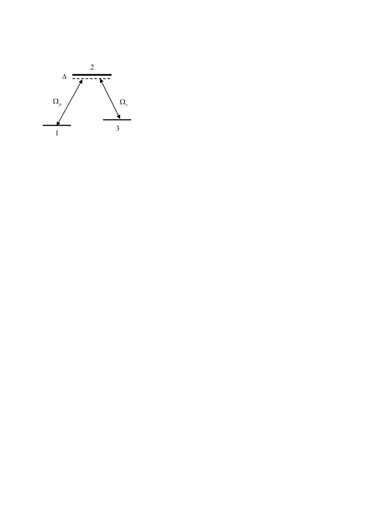
Figure 1: Schematic diagram of the three-level atomic system.

For an exact two-photon resonance, the corresponding Hamiltonian in the resonant approximation (RWA) reads in the basis $\{|1\rangle,|2\rangle,|3\rangle\}$

$$H=\left(\begin{array}[]{ccc}{0}&{-\Omega_{p}^{*}}&{0}\\ {-\Omega_{p}}&{\Delta}&{-\Omega_{s}}\\ {0}&{-\Omega_{s}^{*}}&0\end{array}\right),$$ (1)

with $\Omega_{p,s}=\mu_{p,s}E_{p,s}/2\hbar\equiv|\Omega_{p,s}|e^{i\varphi_{p,s}}$ the Rabi frequencies of the pump and Stokes laser fields, $\mu_{p,s}$ the corresponding dipole moments, $\Delta=\omega_{2}-\omega_{1}-\omega_{p}$ the one-photon detuning. The instantaneous eigenstates write

$$|b_{1}\rangle = \cos\psi\sin\theta e^{-i\varphi_{p}}|1\rangle+\cos\psi\cos\theta e^{-i\varphi_{s}}|3\rangle$$ (2a)

$$+\sin\psi|2\rangle,$$

$$|b_{2}\rangle = \sin\psi\sin\theta e^{-i\varphi_{p}}|1\rangle+\sin\psi\cos\theta e^{-i\varphi_{s}}|3\rangle$$ (2b)

$$-\cos\psi|2\rangle,$$

$$|d\rangle = \cos\theta e^{-i\varphi_{p}}|1\rangle-\sin\theta e^{-i\varphi_{s}}|3\rangle$$ (2c)

with $\Omega^{2}=\left|\Omega_{p}\right|^{2}+\left|\Omega_{s}\right|^{2}$ the generalized Rabi frequency, and the mixing angles defined as $\tan\theta=\left|\Omega_{p}/\Omega_{s}\right|$, $0\leq\theta<\pi/2$ and $\tan 2\psi=2\Omega/\Delta$, $0\leq\psi<\pi/2$ ($0\leq\psi<\pi/4$ if $\Delta>0$). Note that, although for one atom the Rabi frequencies can be taken as real, their phases change in general during the propagation and become complex. The corresponding eigenvalues read

$$\lambda_{b_{1}} = \frac{1}{2}\left(\Delta-\sqrt{4\Omega^{2}+\Delta^{2}}\right)=-\Omega\tan\psi,$$ (3a)

$$\lambda_{b_{2}} = \frac{1}{2}\left(\Delta+\sqrt{4\Omega^{2}+\Delta^{2}}\right)=\Omega\,\text{cotan}\psi,$$ (3b)

$$\lambda_{d} = 0.$$ (3c)

State $|1\rangle$ is connected to the bright state $|b_{1}\rangle$ ($|b_{2}\rangle$) when $\psi\to 0$ ($\psi\to\pi/2$), corresponding to $\Delta>0$ ($\Delta<0$), and $\theta\to\pi/2$ which is satisfied at early times when the pump pulse is switched on first. We will consider without loss of generality $\Delta>0$. The bright state $|b_{1}\rangle$ is up to a phase the state solution during the interaction if the adiabatic conditions are fulfilled:

$$\left|\lambda_{b_{1}}-\lambda_{d}\right| \gg |[i\dot{\theta}-(\dot{\varphi}_{p}-\dot{\varphi}_{s})\cos\theta\sin\theta]\cos\psi|,$$ (4a)

$$\left|\lambda_{b_{1}}-\lambda_{b_{2}}\right| \gg \Bigl{|}i\dot{\psi}+\frac{1}{2}(\dot{\varphi}_{p}\sin^{2}\theta+\dot{\varphi}_{s}\cos^{2}\theta)\sin 2\psi\Bigr{|},\qquad$$ (4b)

where the dot corresponds to the derivative with respect to time. This is satisfied for

$$\left|\Delta T\right|\gg 1,\quad\Omega^{2}T/\left|\Delta\right|\sim\left|\Delta T\right|\psi^{2}\gg 1$$ (5)

with $T$ the time of interaction and $\psi$, $\Omega$ considered during the pulse overlapping. The first inequality means that the spectral width of the pulses should be much smaller than the one-photon detuning, and the second one that this width should be much smaller than the Stark shift of the levels. We have obtained the latter inequality considering the case of interest $\Omega\leq|\Delta|$, which leads to $\sin\psi\sim\psi$ and $\cos\psi\sim 1$. Note that the population of the upper state is proportional to $\psi^{2}$ and in order to reduce the losses from this level (of rate $\Gamma$) one should require additionally

$$\Gamma T\psi^{2}\ll 1.$$ (6)

The Maxwell equations in the running coordinates

$$\eta=x,\;\tau=t-x/c$$ (7)

and in the slowly varying amplitudes approximation read

$$\frac{\partial\Omega_{p}}{\partial\eta}=iq_{p}a_{1}^{*}a_{2},\quad\frac{\partial\Omega_{s}}{\partial\eta}=iq_{s}a_{3}^{*}a_{2}$$ (8)

where $q_{p,s}=2\pi\omega_{p,s}\mu_{p,s}^{2}N/\hbar c$ are the coupling coefficients, with $N$ the atom density in the medium, and $a_{i}$ the atomic population amplitudes determined from the Schrödinger equation

$$i\frac{\partial}{\partial\tau}\phi=H{\rm\;}\phi$$ (9)

with $\phi\equiv[a_{1}\ a_{2}\ a_{3}]^{t}$ ($t$ denotes the transpose). For simplicity, we consider in what follows equal oscillator strengths $q_{p}=q_{s}\equiv q$.

III Effective propagation equations

III.1 First order equations

Combining the Schrödinger equation (9) and the propagation equations (8) leads to

$$\frac{\partial\Omega^{2}}{\partial\eta}=-q\frac{\partial}{\partial\tau}\left|a_{2}\right|^{2},\quad\frac{\partial\Omega_{s}^{*}\Omega_{p}}{\partial\eta}=q\frac{\partial a_{3}a_{1}^{*}}{\partial\tau}.$$ (10)

Using the adiabatic solution of the Schrödinger equation, we get finally the following effective propagation equations for the angles $\theta$, $\psi$ and the relative phase $\varphi=\varphi_{p}-\varphi_{s}$:

$$\frac{\partial\psi}{\partial\eta}+\frac{q}{\Delta^{2}}\cos^{3}2\psi\frac{\partial\psi}{\partial\tau} = 0,$$ (11a)

$$\frac{\partial\theta}{\partial\eta}-\frac{q}{\Omega^{2}}\cos^{2}\psi\frac{\partial\theta}{\partial\tau} = 0,$$ (11b)

$$\frac{\partial\varphi}{\partial\eta}-\frac{q}{\Omega^{2}}\cos^{2}\psi\frac{\partial\varphi}{\partial\tau} = 0.$$ (11c)

This system of equations is valid only when the derivatives at all orders of $\psi$, $\theta$ and $\varphi$ exist and are small such that the adiabatic approximation is satisfied. This excludes in particular field envelopes of bounded domains for which there exist discontinuities of the derivative at a certain order.

We remark that this system of equations (11) contains the time derivative of $\theta$ and $\psi$, and can be thus interpreted as taking into account the first non-adiabatic corrections. We indeed recover these equations starting from the Maxwell equations (10) to which we insert the solution to the Schrödinger equation including the first order non adiabatic corrections, i.e. keeping linear terms in $\partial_{\tau}\theta$ and $\partial_{\tau}\psi$. This calculation can be also interpreted as an adiabatic evolution, not in the usual adiabatic basis, but in the first order superadiabatic basis.

III.2 Solutions

Analytical solutions to (11) can be found by the standard characteristic method Courant :

$$\psi(\eta,\tau)=\psi_{0}(\zeta),\;\theta(\eta,\tau)=\theta_{0}(\xi),\;\varphi(\eta,\tau)=\varphi_{0}(\xi),$$ (12)

where $\psi_{0}(\zeta)\equiv\psi(\eta=0,\tau=\zeta)$, $\theta_{0}(\xi)\equiv\theta(\eta=0,\tau=\xi)$ and $\varphi_{0}(\xi)\equiv\varphi(\eta=0,\tau=\xi)$ are the boundary conditions given at the entrance of the medium, and $\zeta\equiv\zeta(\eta,\tau)$ and $\xi\equiv\xi(\eta,\tau)$ are solutions of the respective equations

$$\zeta = \tau-\eta\frac{q}{\Delta^{2}}\cos^{3}2\psi_{0}(\zeta),$$ (13a)

$$\int_{\zeta}^{\xi}\Omega_{0}^{2}(t)dt = q\eta\cos^{4}\psi_{0}(\zeta)(2-\cos 2\psi_{0}(\zeta))$$ (13b)

with $\Omega(\eta,\tau)=\Omega(\eta=0,\tau=t)\equiv\Omega_{0}(t)$ the generalized Rabi frequency given at the entrance of the medium. The pump and Stokes Rabi frequencies are respectively determined from $\Omega_{p}=\Omega\sin\theta$ and $\Omega_{s}=\Omega\cos\theta$.

Through the definition $\tan 2\psi=2\Omega/\Delta$, Eq. (11a) can be interpreted as describing the dynamics of the generalized Rabi frequency (for a constant $\Delta$) $\Omega(\eta,\tau)=\Omega_{0}(\zeta)$. We conclude that it propagates in the medium through the non-linear time $\zeta$ and with the non-linear velocity $v$ such that $1/v=1/c+q\cos^{3}2\psi_{0}/\Delta^{2}$, smaller than the light velocity $c$, and the delay in the medium for small angles $\psi$ at a certain length $L$ is equal to

$$\tau_{m}=L(1/v-1/c)=\frac{qL}{\Delta^{2}}\cos^{3}2\psi_{0}\sim\frac{qL}{\Delta^{2}}.$$ (14)

From Eq. (13b), the non-linear time $\xi$ is always larger than $\zeta$, meaning that the mixing angle propagates in the medium with the velocity greater than the light velocity Proc ; Li . This can be also inferred from Eq. (11b), where the non linear velocity appears negative.

The solution (12) shows that, if at the medium entrance the relative phase $\varphi$ of the pulses is constant, it remains constant during the propagation in the medium.

III.3 Limitations for the adiabatic passage

We show several limitations of solution (12), all related to the adiabaticity of the process. They can be interpreted in terms of energy leading to the maximum propagation length [see Eq. (16)] and to the maximum time [see Eq. (17)]. Non-adiabatic phenomena that lead to a singularity in the solution, and corresponding to a reshaping of the pulses, are prevented through the limitation (21) [or (22) in the limit of small angle $\psi$]. Reshaping of the pulses is also prevented by (25).

III.3.1 Energy

At the beginning of the interaction $\tau\rightarrow-\infty$, i.e. $\zeta\rightarrow-\infty$ according to Eq. (13a), the quantity $\xi(\eta,\tau\to\ -\infty)$ is estimated by the equation

$$\int_{-\infty}^{\xi(\eta,\tau\to\ -\infty)}\Omega_{0}^{2}(\tau)d\tau\sim q\eta.$$ (15)

We infer that $\xi(\eta,\tau\to-\infty)$ is a monotonic increasing function of $\eta$ changing from $-\infty$ at $\eta=0$ to $+\infty$ at $\eta=\eta_{\max}$, where $\eta_{\max}$ is estimated from

$$\int_{-\infty}^{+\infty}\Omega_{0}^{2}(\tau)d\tau\sim q\eta_{\max}.$$ (16)

This gives a relation between the energy of the pulses and the maximum theoretical propagation length. The physical interpretation of the condition (16) for the length can be expressed in terms of energy: the number of atoms whose population can be fully transferred by adiabatic passage from state $|1\rangle$ to state $|3\rangle$ in the medium cannot exceed the number of photons in the pump and Stokes fields.

III.3.2 Time

The definition of $\zeta$ (13a) shows an additional limitation: For a given length $\eta$, one can get a large value for $\zeta(\eta,\tau)$ when taking a large $\tau$, i.e. when $\tau\gg q\eta/\Delta^{2}$. The definition of $\xi$ (13b) shows then that for a too large $\zeta$, $\xi$ does not exist. For a given $\eta$, the maximum value $\xi\to+\infty$ is obtained for $\tau_{\max}$ estimated from

$$\int_{\tau_{\max}}^{+\infty}\Omega_{0}^{2}(t)dt\sim q\eta.$$ (17)

$\tau_{\max}$ has to be interpreted as a maximum time until which the adiabaticity is preserved. Beyond this value of $\tau_{\max}$, one expects non-adiabatic effects (beyond the first superadiabatic order). Eq. (17) means that, during the propagation corresponding to larger $\eta$, the maximum time from which adiabaticity is broken becomes smaller.

III.3.3 Reshaping of the pulses

Adiabatic conditions (5) have to be revised as follows when considering propagation. The time derivatives in Eq. (4) (in the running coordinates) become:

$$\frac{\partial\psi}{\partial\tau}=\frac{d\psi_{0}}{d\zeta}\frac{\partial\zeta}{\partial\tau},\quad\frac{\partial\theta}{\partial\tau}=\frac{d\theta_{0}}{d\xi}\frac{\partial\xi}{\partial\tau},\quad\frac{\partial\varphi}{\partial\tau}=\frac{d\varphi_{0}}{d\xi}\frac{\partial\xi}{\partial\tau}.$$ (18)

This shows that the adiabatic conditions are the ones at the entrance of the medium provided that

$$\frac{\partial\zeta}{\partial\tau}\leq 1,\quad\frac{\partial\xi}{\partial\tau}\leq 1.$$ (19)

The breaking of these conditions corresponds generally to the formation of shock-waves during the propagation. We obtain for the variable $\zeta$

$$\frac{\partial\zeta}{\partial\tau}=\frac{1}{1-(6q\eta/\Delta^{2})(d\psi_{0}/d\zeta)\cos^{2}2\psi_{0}\sin 2\psi_{0}}.$$ (20)

At large propagation lengths the denominator in the right-hand side of this expression can become very small, that would lead to a strong increase of the derivative of the left-hand side. Thus, in order that the adiabaticity be preserved during propagation it is necessary to add to conditions (5):

$$6\psi_{0}\tan 2\psi_{0}\frac{\tau_{m}}{T}=6\psi_{0}\tan 2\psi_{0}\frac{qL}{\Delta^{2}}\frac{\cos^{3}2\psi_{0}}{T}\ll 1.$$ (21)

We infer that for relatively small angles $\psi$ and propagation lengths $L$ at which the group delay of the generalized Rabi frequency is of the order of the characteristic interaction time, the adiabaticity in the medium does not break down. Considering for simplicity the case of small angles $\psi_{0}$, we get the condition at the length $\eta=L$:

$$qTL\ll\frac{(\Delta T)^{2}}{12}\left(\frac{\Delta}{\Omega_{\max}}\right)^{2}$$ (22)

with $\Omega_{\max}$ the maximum value of $\Omega$. At a given peak Rabi frequency, a larger $\Delta$ allows thus one to increase the medium length for which pulses can propagate without reshaping. One can interpret this effect with the argument that a larger detuning weakens the effective interaction of the pulses with the medium.

With respect to the variable $\xi$, one obtains

$$\frac{\partial\xi}{\partial\tau}=\frac{\Omega^{2}_{0}(\zeta)}{\Omega^{2}_{0}(\xi)}\frac{\partial\zeta}{\partial\tau}\left(1-\frac{6q\eta}{\Delta^{2}}\frac{d\psi_{0}}{d\zeta}\cos^{2}2\psi_{0}\sin 2\psi_{0}\right).$$ (23)

Taking into account the preceding condition (21), this leads to

$$\frac{\partial\xi}{\partial\tau}\sim\frac{\Omega^{2}_{0}(\zeta)}{\Omega^{2}_{0}(\xi)}\frac{\partial\zeta}{\partial\tau}.$$ (24)

This shows that the part $\dot{\theta}$ (and also $\dot{\varphi}$) of the nonadiabatic coupling at the entrance of the medium is multiplied by the scale factor $\Omega^{2}_{0}(\zeta)/\Omega^{2}_{0}(\xi)$ during the propagation. The adiabaticity will break down when this ratio is too large, i.e. when $\xi>\zeta$ for late times. In practice, one can estimate the condition on the propagation length $\eta=L$ by preventing this situation, imposing $\xi-\zeta\ll T$, which gives from Eq. (13b)

$$qTL\ll(\Omega_{\max}T)^{2}.$$ (25)

Inequalities (21) and (25) guarantee the adiabaticity conditions during the pulse propagation, preventing a significant reshaping of the pulses.

IV Population transfer by b-STIRAP

We consider the process of complete population transfer from state 1 to state 3 by adiabatic passage through the bright state using a so-called intuitive sequence of pulses, i.e. with the pump field switched on before the Stokes field with a delay $\tau_{d}>0$. The aim of this section is devoted to the theoretical interpretation of this process. We consider pulses of Gaussian envelopes: $\Omega_{p}=\Omega_{p,\max}\exp[-((t+\tau_{d}/2)/T_{p})^{2}]$, $\Omega_{s}=\Omega_{s,\max}\exp[-((t-\tau_{d}/2)/T_{s})^{2}]$.

The main limitation for an adiabatic transfer for a single atom is given by (5). It gives (i) lower and upper limits for the detuning (at given fields) and (ii) a better adiabaticity for a larger pulse overlapping (that can be achieved with larger Rabi frequencies for given delay and pulse shapes). As studied above, there are four additional limitations given by (16), (17), (21) [or (22) for small angle $\psi_{0}$] and (25). The energetic argument (16) confirms the need of large Rabi frequencies to preserve the adiabaticity during the propagation. The condition (17) on the other hand favours faster processes, i.e. finishing before $\tau_{\max}$. We show below that this is the case for larger detunings. Condition (22) confirms that a larger detuning allows the propagation over a longer distance. Condition (25) is shown below to give the practical limitation on the medium length for which nearly complete population transfer can occur. Due to the interaction with the atoms, the pulses change their shapes. This corresponds to the violation of the adiabaticity conditions, as is studied below. We consider numerical calculations in different situations and interpret them in terms of the limitations described above.

IV.1 Application in experimental conditions

We first apply the analysis to the experiment presented in Exp , for which $\Omega_{p,\max}T_{s}=108.6$, $\Omega_{s,\max}T_{s}=110.5$, $\tau_{d}/T_{s}=1.4$, $T_{p}/T_{s}=0.8$, and $\Delta T_{s}=50$. Figure 2 displays the dynamics of population transfer to state 3 for various lengths $qT_{s}x$ of the medium and the corresponding projections of the state vector $|\phi\rangle$ on the eigenstates. The analytic solution (12) fits well the numerics until the complete transfer fails. The efficiency of the population transfer decreases as the pulses propagate into the medium. The population transfer occurs completely in the medium up to $qT_{s}x\approx 4$. For $qT_{s}x=5$, one can already notice a partial transfer of population.

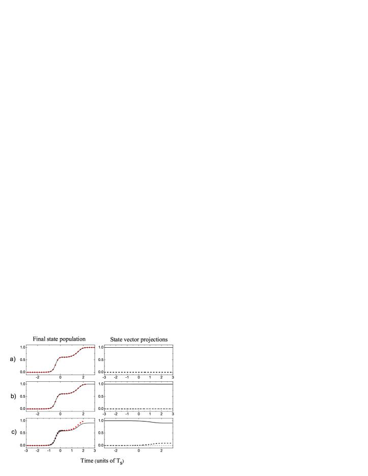
Figure 2: (Color online) For (a) $qT_{s}x=0$, (b) $qT_{s}x=2$, and (c) $qT_{s}x=5$, as a function of the running time $\tau=t-x/c$, left column: Population transfer to state 3 determined numerically (full line) and from the analytical solution (12) (dotted line); right column: Projections $|\langle d|\phi\rangle|^{2}$ (dashed line) and $|\langle b_{2}|\phi\rangle|^{2}$ (dotted line).

Figure 3: Time evolution of the mixing angle $\theta$ for $qT_{s}x=0$ (dashed line) and $qT_{s}x=5$ (solid line). The inset shows an enlargement of the values of the mixing angle near the end of the interaction.

To achieve an effective population transfer one should provide an adiabatic interaction to make state vector $|\phi\rangle$ follow $|b_{1}\rangle$ state and a smooth change of the mixing angle $\theta(\xi)$ from $\pi/2$ to $0$. However, during the propagation, one notices that state vector $|\phi\rangle$ acquires a component along the dark state $|d\rangle$ leading to some final population to state $|1\rangle$. This is clearly seen from the right column of Fig. 2 which shows the instantaneous projections of state vector $|\phi\rangle$ onto the dressed states. We can see that at $qT_{s}x=2$, there is no projections onto states $|b_{2}\rangle$ and $|d\rangle$, while at $qT_{s}x=5$ a noticeable projection onto state $|d\rangle$ appears. As a result the mixing angle $\theta(\xi)$ changes and no more satisfies the conditions that are necessary to realize the transfer process. Indeed, in Fig. 3 we present the time evolution of the mixing angle $\theta(\xi)$ for the same parameters as in Fig. 2. One can see that already at propagation length $qT_{s}x=5$ the final value of $\theta(\xi)$ is different from $0$.

IV.2 Interpretation and improvement of the transfer

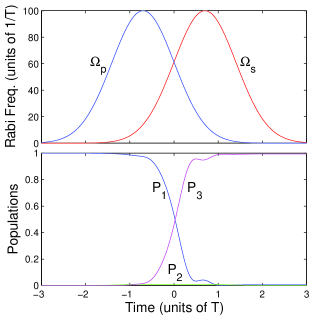
Figure 4: (Color online) Dynamics of the population transfer $P_{j}=|\langle j|\phi\rangle|^{2}$ (lower frame) corresponding to the pulses (upper frame) at the entrance of the medium $x=0$ for $T\Delta=1000$ and $T\Omega_{p,\max}=T\Omega_{s,\max}=100$.

To interpret the maximal length leading to the complete transfer and to show how to improve it, we analyze the transfer taking similar parameters of the experiment. We take for simplicity equal peak Rabi frequencies and equal durations for both pulses.

The main limitation is here given by Eq. (17). It shows indeed that a process corresponding to a population transfer lasting too long, i.e. beyond $\tau_{\max}$, leads to an inefficient non-adiabatic transfer when propagation is considered. To illustrate this effect, we consider below two limiting cases with the same Rabi frequencies and pulse durations ($\Omega_{p,\max}=\Omega_{s,\max}$, $T_{p}=T_{s}=T$), the delay $\tau_{d}=1.3T$, and satisfying (5): one with a large detuning defined as $\Delta\gg\Omega_{\max}$ (see Fig. 4), leading to a negligible population in the intermediate state, and another one with a small detuning defined as $\Delta\sim\Omega_{\max}$ (see Fig. 5), leading to a noticeable population in the intermediate state. At the entrance of the medium, $\eta=0$, the population transfer for the large detuning case is accomplished approximately during the overlap of the pulses (see Fig. 4), while, for the small detuning, it occurs for the duration of both pulses (see Fig. 5). (The calculation with the small detuning corresponds to conditions that are very similar to the experiment described above.) Thus condition (17) is easier to satisfy for a larger detuning. The effect that the transient population in the intermediate state is smaller for a larger $\Delta$ corresponds to a weaker interaction of the pulses with the medium, and the condition (21) [or (22)] is also easier to satisfy. One thus expects an adiabatic transfer over much longer propagation length for the case of large detuning. This is confirmed by the numerics. Figure 6 shows that, already for $qTx=7$, the population transfer is not complete. One can see that the corresponding analytic solution fits well the numerics (until it stops at $\tau\approx 2.35T$), before the Stokes pulse is off and the transfer is complete. This time corresponds with a quite good approximation to the one determined from the estimation (17) giving $\tau_{\max}\approx 2.33T$. Figure 6 shows that the nonadiabatic corrections correspond to a projection onto the dark state that grows roughly monotonically as a function of time, reaching its peak value near $\tau_{\max}$.

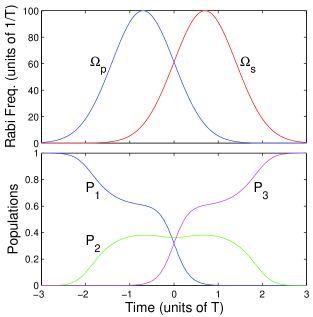
Figure 5: (Color online) Same as Fig. 4 but for $T\Delta=50$ and $T\Omega_{p,\max}=T\Omega_{s,\max}=100$.

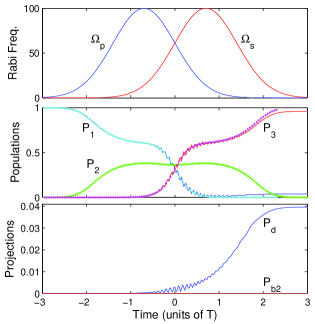
Figure 6: (Color online) Dynamics of the population transfer $P_{j}=|\langle j|\phi\rangle|^{2}$ (middle frame) for $T\Delta=50$, $T\Omega_{p,\max}=T\Omega_{s,\max}=100$ and at $qTx=7$ (corresponding to Fig. 5 for $x=0$); the absolute value of the corresponding Rabi frequencies (upper frame); and its corresponding non-adiabatic projections onto the dark state $P_{d}=|\langle d|\phi\rangle|^{2}$ and the bright state $P_{b_{2}}=|\langle b_{2}|\phi\rangle|^{2}$. The dotted lines for the populations are determined from the analytic solution (12), (13).

For the large detuning case, the limitation of the population transfer during the propagation is given by (25). Figure 7 shows the dynamics for $qTx_{\max}=100$ which corresponds roughly to the maximum length with an efficient population transfer (it reaches here approximately $99\%$). With respect to the condition (25), this corresponds to $qTL/(\Omega_{\max}T)^{2}=0.01$. Inspection of the obtained pulse shows that this non-adiabatic effect occurs near the end of the pump pulse, where it is significantly reshaped featuring a longer tail. Such a reshaping breaks the initial intuitive sequence of the pulses since when the Stokes falls down the pump pulse is not any more completely switched off. Figure 7 shows that the nonadiabatic corrections correspond to a projection onto the dark state. The maximal length obtained for the large detuning case is well beyond the one obtained for the small detuning case as discussed above.

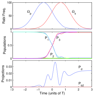
Figure 7: (Color online) Same as Fig. 6 but for $T\Delta=1000$ and $T\Omega_{p,\max}=T\Omega_{s,\max}=100$ and at $qTx=100$ (corresponding to Fig. 4 for $x=0$). The small discrepancy between numerics and the analytic solution is due to nonadiabatic corrections of order higher than one.

We conclude that in order to increase the propagation length for given identical pump and Stokes peak amplitudes, besides taking large detuning $\Delta$ [in the limit of Eq. (5)], we should take the delay between the pulses as large as possible, while keeping an overlapping between the two Rabi frequencies of sufficiently large area (much bigger than one).

We remark that the obtained maximum lengths of the medium where the complete population transfer occurs are here well below the lengths that would lead to a singularity in the pulse shapes, as given by condition (22).

IV.3 Practical implementation and examples

Equations (5) and (6) are the conditions that must be met in order to achieve an efficient population transfer by b-STIRAP in a medium. We consider below various media and experimental conditions that satisfy these conditions.

In the gas phase, the limitations imposed by the losses from the three-state system are mainly due to the inhomogeneous linewidth of the excited state [through Eq. (6)] and to the ionization by the fields, mainly from the excited state. In the case of a warm vapor, the inhomogeneous linewidth is mainly determined by the Doppler broadening, typically $\Gamma=500$MHz for a warm alkali-metal-atomic vapor. In a regime corresponding to $\Omega\sim\Delta$, leading to a relatively short propagation length and a quite large transient population in the excited state as typically shown in Figs. 6 and 9, all the criteria are fulfilled for a pulse duration of order $T=40$ ps. In the conditions of Fig. 9, we have $\Omega=\Delta/2$, $(\Omega/\Delta)^{2}\Gamma T=0.005$ (corresponding to a negligible loss), $\Delta T=40$, $\Omega^{2}T/\Delta=10$ and $\Omega=500$ GHz. This imposes to find a particular system with a limited ionization from the excited state with such a Rabi frequency, which corresponds to typical intensities of 30 MW/cm² (for a transition strength of order of one Debye). For a long propagation length regime (as typically shown in Fig. 7, for $\Omega/\Delta=0.1$) with a small transient population in the excited state, one obtains $T=1$ ns as the typical pulse duration. In the conditions of Fig. 7, this gives $(\Omega/\Delta)^{2}\Gamma T=0.005$, $\Delta T=1000$, and $\Omega^{2}T/\Delta=100$ corresponding to the Rabi frequency $\Omega=100$ GHz, i.e. to a generally weakly ionizing field of 1 MW/cm² (for a transition strength of order of one Debye). We remark that such a situation leads to $\Gamma T\sim 0.5$. However it is not expected to give a large loss due to the small transient population in the upper state (of order $(\Omega/\Delta)^{2}\sim 0.01$). We have checked numerically this assumption as shown in Fig. 8, where various loss rates are studied. The loss rate $\Gamma T=0.1$ does not show a noticeable loss in the process, while the loss rate $\Gamma T=0.5$ gives a small loss of less than 3 percents.

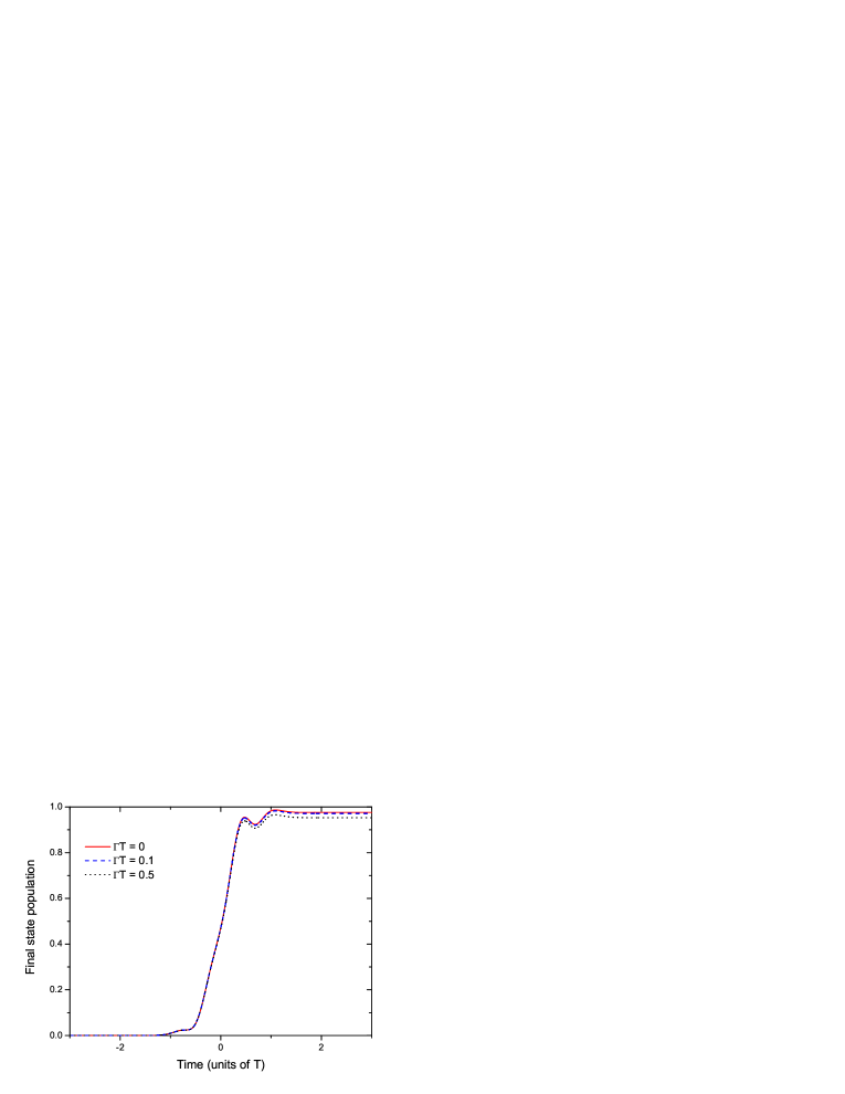
Figure 8: (Color online) Population transfer in the conditions of Fig. 7 but for various loss rates: $\Gamma T=0$ (full line), $\Gamma T=0.1$ (dashed line, almost undistinguishable from the full line) and $\Gamma T=0.5$ (dotted line).

The situation is less restrictive in cold medium (such as Bose Einstein Condensates system) where $\Gamma$ is bounded by the natural rate of losses from the excited state which is of order of 10 MHz. In this case the pulse duration can be increased to $T\sim 2$ ns for the short propagation length regime case ($\Delta\sim\Omega$) and to $T\sim 50$ ns for the long propagation length regime $\Omega/\Delta\sim 0.1$. In these cases, the Rabi frequencies range from $\Omega\sim 2$ GHz to $\Omega\sim 20$ GHz which are well below the ionization regime in general.

For solids, one of the main additional difficulties comes from their large optical inhomogeneous broadening. For example, in rare-earth-doped crystals, that are preferable within the context of coherent optical behavior for $f-f$ transitions, the upper state inhomogeneous broadening is of the order of 10 GHz. However, there are some techniques like hole-burning techniques that allow one to select a subset of the ions within a particular spectral range and thus to reduce the large inhomogeneous broadening. This allows one to increase the pulse durations up to the microsecond regime. This technique has been used in the experiment of Ref. Exp that we have taken to apply our theoretical results (see Sec. IV A). There is usually another issue due to the level splitting $\Delta_{S}$ in ”atom-like” systems (doped solids, color centers, quantum dots) in the range of 10 MHz - 10 GHz. This gives limits for the Rabi frequencies to address single levels: $\Omega\ll\Delta_{S}$.

V Pulse dynamics and reshaping

We here show the dynamics of the intuitive pulse sequence propagating in the medium over long distance beyond adiabatic limitations. We choose parameters that show a reshaping already for small distances in the medium: $\Omega_{\max}T=20$, $\tau_{d}/T=1$, and $\Delta T=40$.

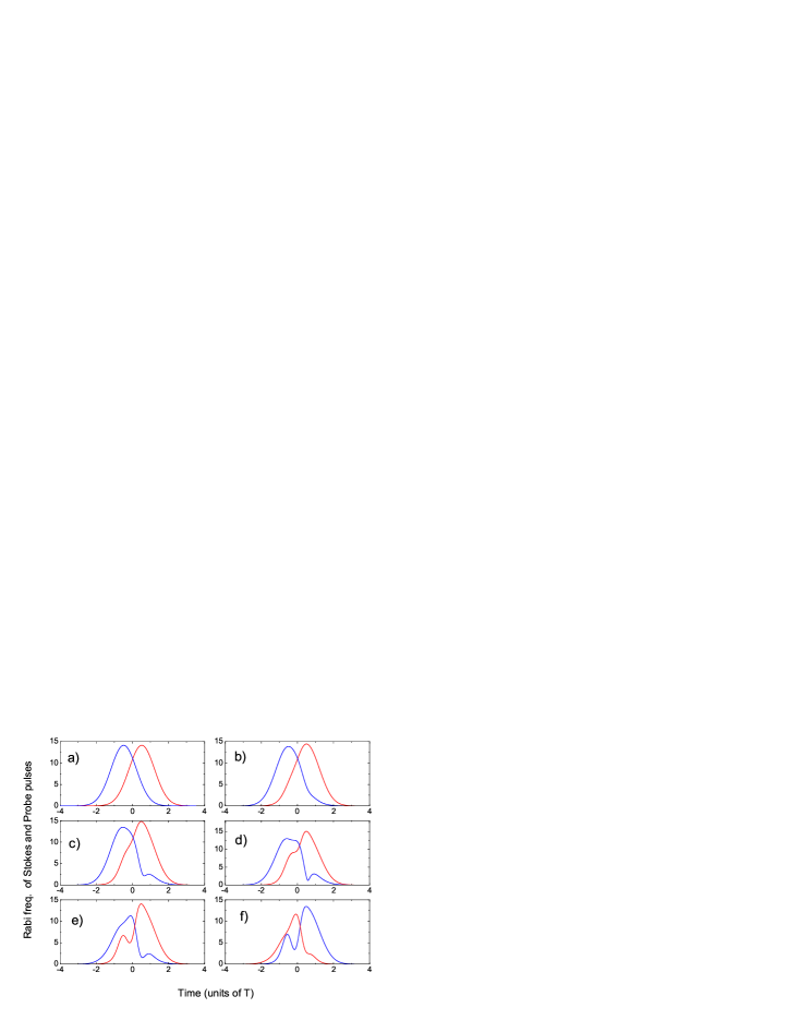
Figure 9: (Color online) Time evolution of the normalized Rabi frequencies of the probe and Stokes pulses for different propagation lengths $z\equiv qTx$: a) z = 0; b) z = 10; c) z = 20; d) z = 30; e) z=40; f) z=50.

Figure 9 shows a typical dynamics: After a certain length there occurs a noticeable reshaping corresponding to a lengthening of the shape of the pump intensity at the tail leading to additional peaks (here one peak is shown). Already for $z=10$, the population transfer is not anymore complete in this situation. The adiabaticity is strongly violated beyond this value. The leading edge of the stokes pulse is next also reshaped also showing one additional peak. The sequence of pulses is not any more intuitive at large distances.

VI Conclusion and discussion

We have analyzed the complete population transfer by adiabatic passage when the pulses propagate in a medium in an intuitive sequence. Using the analytic solution, determined from the first order nonadiabatic corrections, we have derived limitations on the maximal length of the medium where the complete population transfer can take place. Assuming the adiabatic conditions fulfilled at the entrance of the medium [see conditions (5)], the complete population occurs over a longer distance in the medium (i) for a larger one-photon detuning (at given peak Rabi frequencies of the pulses) and (ii) for a larger peak Rabi frequency of the pulses (at a given ratio of the one-photon detuning with the peak Rabi frequency of the pulses). In the limit $\Delta\gg\Omega$, the limitation of the transfer appears as non-adiabatic corrections and a reshaping of the pump pulse through the condition (25).

We can list the differences between the techniques of STIRAP and b-STIRAP. Unlike STIRAP, b-STIRAP depends on the one-photon detuning. Increasing the one-photon detuning leads to an improvement of the propagation length at which the population transfer is complete in a medium. On the other hand, increasing the one-photon detuning weakens the adiabaticity of the interaction.

The second difference concerns the derived criteria of adiabaticity in a medium. During the propagation of the two pulses there is an exchange of energy between them that causes their reshaping which breaks down the adiabaticity. For a counterintuitive pulse sequence, in the case of equal oscillation strengths, the adiabaticity is preserved during propagation at any propagation length. Only in the case of unequal oscillator strengths it can break down, mainly due to a singularity corresponding to a steepness occurring in the shape of the pulse (see STIRAPmedium ; Fleisch ). In the case of an intuitive pulse sequence as shown in the present work the adiabaticity is broken down in a medium even for equal oscillator strengths.

As noticed very recently Proc ; Li , an intuitive sequence of the switching of the pulse features a reshaping that can lead to a superluminal propagation Superl1 ; Superl2 ; Superl3 ; Superl4 . Our analytic solution should provide new insights about this effect and its limitation. Such a study is in progress.

b-STIRAP can be viewed as an alternative population transfer method. The superluminal property of b-STIRAP can find applications. For instance, the simultaneous use of the b-STIRAP and STIRAP processes in multi-level systems (e.g. tripod, M-system) can be an efficient method for creating time controlled excitations of target states. We also anticipate that a combination of STIRAP/b-STIRAP is of interest in quantum information. The counterintuitive STIRAP scheme indeed allows the population to be transferred from 1 to 3 - while the same pulse sequence permits transfer back from 3 to 1 in an intuitive b-STIRAP scheme. This could find applications for the implementation of quantum gates.

Appendix A Method of characteristics for $\psi$ and $\theta$

In this appendix we derive the solution of Eqs. (11) of the form

$$\frac{\partial\psi}{\partial\eta}+a(\psi)\frac{\partial\psi}{\partial\tau} = 0,$$ (26a)

$$\frac{\partial\theta}{\partial\eta}-b(\psi)\frac{\partial\theta}{\partial\tau} = 0,$$ (26b)

using the method of characteristics Courant . We first solve Eq. (26a) using a characteristic parametrization $\eta\equiv\eta(s)$ and $\tau\equiv\tau(s)$ such that

$$\frac{d\psi}{ds} = 0,$$ (27a)

$$\frac{d\eta}{ds} = 1,$$ (27b)

$$\frac{d\tau}{ds} = a(\psi).$$ (27c)

$\psi$ is constant along the characteristics: $\psi(\eta,\tau)=\psi(\eta(0),\tau(0))$. From (27b), we get $\eta(s)=s$ choosing $\eta(0)=0$. This entails

$$\psi(\eta,\tau)=\psi(0,\zeta)\equiv\psi_{0}(\zeta),\quad\zeta\equiv\tau(0)$$ (28)

with $\zeta\equiv\zeta(\eta,\tau)$ solution of Eq. (27c):

$$\zeta=\tau-\eta a(\psi_{0}(\zeta)).$$ (29)

This leads to Eq. (13a).

We next solve Eq. (26b) rewritten as

$$\frac{\partial\theta}{\partial z}-\frac{a(\psi_{0})+b(\psi_{0})}{1+za^{\prime}(\psi_{0})\psi_{0}^{\prime}(\zeta)}\frac{\partial\theta}{\partial\zeta}=0$$ (30)

using the change of variables

$$z=\eta,\quad\zeta=\tau-\eta a(\psi_{0})$$ (31)

and denoting $a^{\prime}(\psi_{0})\equiv da/d\psi_{0}$, $\psi_{0}^{\prime}(\zeta)\equiv d\psi_{0}/d\zeta$. The method of characteristics allows one to solve Eq. (30):

$$\theta(\eta,\tau)=\theta(0,\xi)\equiv\theta_{0}(\xi),\quad\xi\equiv\zeta(0)$$ (32)

with $z(s)=s$ and

$$\frac{d\zeta}{ds}=-\frac{a(\psi_{0})+b(\psi_{0})}{1+sa^{\prime}(\psi_{0})\psi_{0}^{\prime}(\zeta)}.$$ (33)

The solution of the latter equation reads

$$s = \int_{\zeta}^{\xi}\frac{d\zeta^{\prime}}{a[\psi_{0}(\zeta^{\prime})]+b[\psi_{0}(\zeta^{\prime})]}$$ (34)

$$\times\exp\left[\int_{\psi_{0}(\zeta)}^{\psi_{0}(\zeta^{\prime})}d\psi_{0}^{\prime}\frac{a^{\prime}(\psi^{\prime}_{0})}{a(\psi^{\prime}_{0})+b(\psi_{0}^{\prime})}\right],$$

which gives Eq. (13b).

References

- (1) K. Bergmann, H. Theuer, and B.W. Shore, Rev. Mod. Phys. 70, 1003 (1998);
- (2) M. Ter-Mikayelyan, Phys. Usp. 40, 1195 (1997).
- (3) N.V. Vitanov, T. Halfmann, B.W. Shore, and K. Bergmann, Annu. Rev. Phys. Chem. 52, 763 (2001).
- (4) A.T. Nguyen, G.D. Chern, D. Budker, and M. Zolotorev, Phys. Rev. A 63, 013406 (2000).
- (5) G.G. Grigoryan and Y.T. Pashayan, Phys. Rev. A 64, 013816 (2001).
- (6) H. Goto, K. Ichimura, Phys. Rev. A 74, 053410 (2006).
- (7) H. Goto, K. Ichimura, Phys. Rev. A 75, 033404 (2007).
- (8) J. Klein, F. Beil, and T. Halfmann, Phys. Rev. Lett. 99, 113003 (2007); Phys. Rev. A 78, 033416 (2008).
- (9) N.V. Vitanov, S. Stenholm, Phys. Rev. A 55, 648 (1997).
- (10) L.P. Yatsenko, S. Guérin, and H. R. Jauslin, Phys. Rev. A 65, 043407 (2002).
- (11) R. Courant, Partial Differential Equations (Interscience publishers, New York, 1962).
- (12) M. Fleischhauer, A. Imamoglu, and J.P. Marangos, Rev. Mod. Phys. 77, 633 (2005).
- (13) G.G. Grigoryan, G. Nikogosyan, and T. Halfmann, arXiv:0901.4210v1 [physics.atom-ph].
- (14) H.J. Li, C. Hang, G. Huang, and L. Deng, Phys. Rev. A, 78, 023822 (2008).
- (15) L.J. Wang, A. Kuzmich and A. Dogariu, Nature 406, 277 (2000).
- (16) A. Dogariu, A. Kuzmich, H. Cao, L. J. Wang, Optics Express 8, 344 (2001).
- (17) L. Deng, M. G. Payne, PRL 98, 253902 (2007); K. J. Jiang, L. Deng, M. G. Payne, Phys. Rev. A 76, 033819 (2007).
- (18) K. J. Jiang, L. Deng, E. W. Hagley, M. G. Payne, Phys. Rev. A 77, 045804 (2008).