Spectroscopic Observations of Hot Lines Constraining Coronal Heating in Solar Active Regions

Abstract

EUV observations of warm coronal loops suggest that they are bundles of unresolved strands that are heated impulsively to high temperatures by nanoflares. The plasma would then have the observed properties (e.g., excess density compared to static equilibrium) when it cools into the 1-2 MK range. If this interpretation is correct, then very hot emission should be present outside of proper flares. It is predicted to be vey faint, however. A critical element for proving or refuting this hypothesis is the existence of hot, very faint plasmas which should be at amounts predicted by impulsive heating. We report on the first comprehensive spectroscopic study of hot plasmas in active regions. Data from the EIS spectrometer on Hinode were used to construct emission measure distributions in quiescent active regions in the 1-5 MK temperature range. The distributions are flat or slowly increasing up to approximately 3 MK and then fall off rapidly at higher temperatures. We show that active region models based on impulsive heating can reproduce the observed EM distributions relatively well. Our results provide strong new evidence that coronal heating is impulsive in nature.

1 Introduction

Almost 10 years ago it was realized that warm ($\approx$ 1 MK) active region (AR) loops seen in the EUV cannot be explained by static equilibrium theory. For example the observations showed that these loops are appreciably more dense than what static loop models would predict (e.g., Aschwanden, Schrijver $\&$ Alexander 2001; Winebarger, Warren $\&$ Mariska 2003; Warren, Feldman $\&$ Brown 2008; Warren et al. 2008).

It was thus proposed that coronal loops could be collections of unresolved strands which are heated impulsively by small-scale heating events (i.e. nanoflares) to high temperatures of several MK which then cool down to the 1 MK range to give rise to the observed EUV loops (e.g., Cargill 1993; and the review of Klimchuk 2006 and references therein). This paradigm proved quite successful at reproducing several key observational aspects of the 1 MK loops (e.g. Klimchuk 2006). Note here that impulsively heated sub-resolution strands can also be invoked to explain the emissions from areas not containing resolved coronal loops, i.e., diffuse background areas. The primary difference between loops and background could be that for loops, nanoflares occur in a somewhat coordinated fashion over a distance comparable to the loop diameter, whereas for the background, they occur at rather random times and with a broader spatial distribution.

However, the details of the heating process are essentially lost by the time an impulsively heated loop cools though the 1 MK range (e.g., Winebarger $\&$ Warren 2004; Patsourakos $\&$ Klimchuk 2005; Parenti et al. 2006). Therefore, one has to search for signatures of the postulated impulsive heating in higher temperature emissions in order to prove or refute this picture of coronal heating. Observing in spectral lines is preferable, since they are formed over a rather narrow temperature range which allows a more precise and unambiguous temperature determination compared to narrow and broad band imaging. Observations in hot emissions could then be viewed as a true “smoking gun” of the impulsive heating (e.g., Cargill 1995; Patsourakos and Klimchuk 2006). One difficulty with observing the hot spectral emissions is that they are predicted to be quite faint (e.g., Patsourakos $\&$ Klimchuk 2006; Bradshaw $\&$ Cargill 2007; Reale $\&$ Orlando 2008; Klimchuk, Patsourakos, & Cargill 2008). Moreover, there exist very few observations of hot spectral emissions in quiescent active regions taken with desirable spatial resolution.

With this work we address the following important questions. Is there any evidence of the elusive hot line emissions? Are there any spectroscopic signatures of hot ($>$ 3 MK) loops in ARs? And are the intensities in hot lines consistent with the predictions of impulsively heated models? It is very timely to address these questions, given the availability of the new, high-quality data-stream from the Extreme Ultraviolet Imaging Spectrometer (EIS) of Hinode. In particular, the larger effective area of EIS compared to its predecessors is critical for observing the important yet faint hot line emissions.

2 Observations and Data Analysis

EIS (Culhane et al. 2007; Korendyke et al. 2006) is an imaging spectrometer operating in two ranges of the EUV (171-212 Å  and 245-291 Å). These windows contain spectral lines formed in the range $\approx$ 0.05-15 MK. Our observations were taken from 22:40-23:35 UT on 30 June 2007; EIS study HPW008_FULLCCD_RAST. 128 steps of the scanning mirror were made, with 30 s exposures taken at each slit position. The pixel size is 1 $\mathrm{{arcsec}^{2}}$. An area of 128$\times$128 $\mathrm{arcsec^{2}}$ was rastered and full CCD readouts were sent to Earth. The target was a small and simple active region (NOAA AR 10961) not very far from disk center. The raw data were processed with the standard eis_prep routine which among other things subtracts the dark current, identifies hot, warm and dusty pixels, and finally applies the absolute photometric calibration to the data.

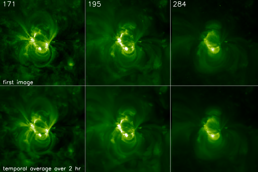
Figure 1: Images in the 171, 195 and 284 channels of EUVI of STEREO A taken around 22:00 UT on 30 June 2007 (upper panel) and temporal average of all corresponding images for the same channels for the time interval of $\approx$ 22-24 UT on 30 June 2007 (lower panel). The square root of intensity is displayed. Same scaling is applied to images from the same wavelength.

The target AR did not evolve substantially during our observations. Inspection of Hinode XRT (Golub et al. 2007) and STEREO SECCHI/EUVI (Howard et al. 2007) movies in SXR and the EUV respectively revealed a number of distinct loops, most of which were visible during the entire time of the EIS raster. The upper panels in Figure 1 show images in the 171, 195 and 284 channels of EUVI (from the Ahead STEREO spacecraft) taken around 22:00. The lower panels show corresponding averages of co-aligned images from the interval 22:00-24:00. The similarity in the appearance of the instantaneous snapshot and time average for each channel is indicative of a lack of major evolution.

To quantify this, in Figure 2 we plot the time evolution of the maximum intensities in the observed AR for the 171 ($\approx$ 1 MK) and Tipoly ($\approx>$ 5 MK) channels of EUVI and XRT respectively. We see that the maximum intensities do not vary by more than $\approx$ 20-30 $\%$ during the 1 hr of our observations. The variation in the spatially averaged intensities is even less. Note that the pixel of maximum intensity changes location every 2-4 exposures, an indication that some variability is present.

It is important to stress that the lack of perceived evolution does not preclude the possibility that dramatic changes are happening on a subresolution scale. In particular, if loops and/or the diffuse background are heated by nanoflares within unresolved strands, then the strands will be evolving rapidly even when the observed large-scale structures appear to be steady.

For further analysis we selected a series of well-defined warm and hot lines formed in the temperature range $\approx$ 1-5 MK (Table 1). We used line identifications proposed by the EIS team (Young et al. 2007; Brown et al. 2008; Del Zanna 2008; Warren et al. 2008). Significant effort has has been made to identify ”clean” hot lines in the EIS wavelength range (Del Zanna 2008; Warren et al. 2008), and such lines are used in our analysis.

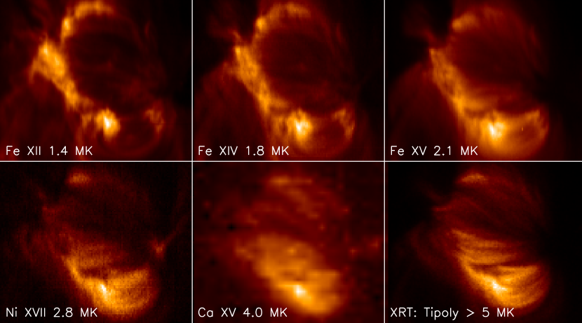
Figure 3: Images of the observed AR in 5 spectral lines observed by EIS and in the Tipoly channel of XRT. Square root of intensity is displayed, and each image is scaled individually. Formation temperatures are indicated. The observed field is 128$\times$111 $\mathrm{{arcsec}^{2}}$, and spatial shifts between EIS data recorded in the 2 different CCDs have been corrected.

Images of the AR in several of the lines are displayed in Figure 3, together with a Tipoly image from XRT. For the strong and isolated Fe XII, Fe XIV, Fe XV, and Ni XVII lines the images were constructed by simply integrating the background subtracted profiles at each pixel. For Ca XV we first binned the data in 2$\times$2 pixels to increase the signal-to-noise ratio. Then, for each macro-pixel we employed a two-Gaussian fit to account for a nearby Fe XIII line at $\approx 201.12$ Å.

Several remarks can be made about morphology of the hot plasma seen in Figure 3. The emission in Ca XV (4 MK) is rather widespread in the active region and not just concentrated in a small number of discrete features. A few rather fuzzy loop structures are discernable. The overall morphology in this line is similar to that seen in the broad-band XRT image in the Tipoly channel which is sensitive to plasmas $\approx>$ 5 MK. Note however that the XRT image looks sharper than the Ca XV image. This is due partly to the higher signal-to-noise ratio of XRT data (XRT is a broad-band instrument while EIS takes monochromatic images over small wavelength windows) and partly to the higher spatial resolution of XRT. The Ca XV image also seems smoother because of the 2$\times$2 pixel binning.

Unfortunately, the signal in the remaining hot lines at single pixels or macro-pixels of reasonable size (e.g. 2$\times$2, 4$\times$4) is too faint to construct images like we did for the lines shown in Figure 3. For example, the strongest Fe XVII line is about 100 times fainter than the Fe XII line at 195.12 Å. We therefore computed an average profile over the entire AR for each of the lines of Table 1. We then fitted the average profile with one or two Gaussians plus a linear background (a double Gaussian was used when another line was in the vicinity of the line of interest). Finally, we determined an average intensity from the fit.

It was necessary to account for two effects before combining the profiles to obtain the averages. First, the two wavelength ranges of EIS are imaged on separate CCD detectors, and there is a relative offset of $\approx$ 2 and 17 pixels in the x and y directions. We restricted our averages to the common parts of the two detectors. Second, the spectral lines exhibit a quasi-periodic drift that is believed to be caused by thermal variations of the spacecraft during its $\approx$ 90 min orbit. The amplitude of the drift corresponds to a Doppler shift of several 10 $\mathrm{km/s}$. We corrected for this effect in the following manner (see also Warren et al. 2008). First, we determined the centroid (first moment) of the strong Fe XII line at 195.12 Å  at each location along the slit. Then, we calculated the average centroid along the slit for each raster position. Finally, we interpolated between the slit averages to determine the wavelength correction as a function of time. This makes the implicit assumption that the observed drifts of the spectral lines are not of solar origin. We verified the robustness of the above process by: (1) repeating it for another strong line (Fe XV 284.16 Å) which is recorded on the other CCD and is formed at a different temperature; (2) computing the centroid of the slit-averaged profile at each raster position, rather than the average centroid of individual profiles. In both cases, the deviation from the original scheme does not exceed a few $\mathrm{km/s}$.

As a last step in the analysis, we calculated the emission measure distribution $EM(T)$ of the AR using the spatially averaged intensities and the latest version of CHIANTI v5.2 (Dere et al. 1999; Landi et al. 2006). We made the usual assumption that the bulk of the line emission originates from a temperature interval $\Delta\log T=0.3$ that is centered on the temperature of peak formation. This was shown to be a reasonable assumption even for complex plasma distributions like those from impulsively heated models (Klimchuk $\&$ Cargill 2001). Notice that the employed ions (Fe, Ca and Ni) all have a low First Ionization Potential, and therefore the relative intensities should be largely independent of the assumed set of elemental abundances. We chose the abundances of Feldman (1992). Finally, error bars in the determined $EM$ were calculated by quadratically combining the errors in the fitted intensities plus a 30$\%$ uncertainty in the photometric calibration of EIS, based on pre-flight measurements (Culhane et al. 2007).

The $EM$ distribution of AR 10961 is shown in Figure 5. The distribution is relatively flat in the temperature range from $\approx$ 1-4 MK, and then falls off by almost a factor of 10 at our hottest line at 5.0 MK. Lines formed at similar temperatures are generally consistent to within the error bars (vertical lines), though small discrepancies remain that may be due to uncertainties in the atomic physics.

To determine whether this distribution is typical of most active regions, we repeated our analysis on 8 additional datasets obtained between January and September 2007. Only a subset of the lines in Table 1 were used: Fe XII, Fe XV, Ni XVII and Fe XVII (254.87 Å ). The results are shown in Figure 6. In all cases, the $EM$ distribution is either flat or mildly increasing up to 3 MK and falls off by 1-1.5 orders of magnitude at 5 MK. Similar distributions have been reported from smaller datasets (e.g., Brosius et al. 1996; Watanabe et al. 2008). It is intriguing that the $EM$ of the coolest line, Fe XII formed near 1.4 MK, varies by only a factor of 2-3 for all of our examples, whereas the $EM$ of the hottest line, Fe XVII, is much more variable. The ratio of the two lines ranges from $\approx$ 5-50. This suggests that hot emissions are the most sensitive indicators of the coronal heating mechanism, as indicated above and discussed shortly.

Before proceeding, we return to the question of whether spatially averaged intensities are representative of active regions as a whole, especially for faint hot plasmas. For instance, a transient brightening and/or a localized bright spot may dominate the averages. We can rather safely exclude this possibility for the following reasons. First, the light curves of Figure 2 show that no appreciable brightening took place during the observations of AR 10961. Second, the hot Ca XV emission is widely distributed throughout the active region (Figure 3). We have confirmed that the conspicuous bright spot in the lower middle part of the image does not greatly influence the average. Third, we have performed sit-and-stare observations of this active region in the even hotter Fe XVII lines (maintaining a single slit position for $\approx$ 1 hour). There is significant emission along most of the slit, with enhancements in places that are known to cross loops observed in warmer lines like Fe XV.

Knowing how distinct loops and the diffuse background contribute to the total emission from an active region is an important question that has been largely overlooked. Figure 4 shows a vertical intensity cut through the middle of the Fe XII image of 3. There are a few local intensity maxima (e.g. around solar-y 15, 30, 40) which can be identified with distinct loops. However, these resolved loops do not stand out appreciably above the background (they produce an intensity enhancement of only 10-30 $\%$) and they occupy a rather small fraction of the AR volume. Therefore, we expect that the diffuse background contributes more to our spatially averaged intensities and $EM$ distributions than do distinct loops. Of course part of the background could represent indistinguishable, overlapping loops. More work is needed on this important question.

3 Modeling

A major goal of our study is to determine whether the observations support or contradict impulsive coronal heating. We therefore calculated the $EM$ distribution expected from a simple model active region that is heated by nanoflares. We used our 0D hydrodynamic simulation code called EBTEL, described in full by Klimchuk, Patsourakos $\&$ Cargill (2008). For a given temporal profile of the heating, EBTEL calculates the evolution of $EM(T)$ for both the coronal and footpoint (i.e., transition region; TR) sections of a stand. The inclusion of the TR emission in spatially averaged intensities is important, since it can dominate the emission at temperatures up to 1-2 MK or even higher, depending on the magnitude of the nanoflare. EBTEL mimics complex 1D hydrodynamic simulations very well (Klimchuk et al. 2008), but uses orders of magnitude less computer time and memory. Note that impulsively heated AR models are able to reproduce some of the salient morphological features of ARs like the bright SXR core and the extended EUV loops (Warren $\&$ Winebarger 2007; Patsourakos $\&$ Klimchuk 2008).

We calculated hydrodynamic models for 26 stands with lengths in the range 50-150 Mm, pertinent to the sizes of macroscopic loops in AR 10961. This model is a good approximation considering the rather simple, bipolar nature of the AR. We started with static equilibria having an average coronal temperature near 0.5 MK. We heated the strands with a triangular pulse lasting 50 s and let the strands cool for 8500 s, by which time the temperature had cooled below 1 MK. The amplitude $H$ of the heat pulses varied from strand to strand according to

$$H=H_{0}{(L/L_{0})}^{\alpha},$$ (1)

with $H_{0}$ the heating magnitude, $L_{0}$ the length of the shortest loop, and $\alpha$ a scaling-law index that is related to the specific mechanism of heating. We chose $\alpha=-2.8$, which is appropriate for heating that occurs when a critical shear angle is reached in a magnetic field that is tangled by photospheric convection (Mandrini et al. 2001; Dahlburg et al. 2005).

Following Klimchuk (2006) we time-averaged the $EM$ distributions for each strand simulation to approximate a snapshot observation of either a multi-stranded macroscopic coronal loop or an unstructured background area. These individual distributions were then added together to get a final $EM$ distribution for the entire active region. Note that the heating magnitude $H_{0}$ of Equation 1 was chosen to yield an $EM$ at warm ($\approx 1-2$) MK temperatures that agrees with observed values. Previous studies attempting to reproduce coronal loop observations in warm emissions adopted a similar strategy. The open question has been whether the hot line intensities predicted by the models are consistent with observations. We here provide the first ever check of this type.

The solid curve in Figure 5 is the $EM$ distribution for our model active region. It agrees very well with the EIS observations in the temperature range 1-5 MK for which we have data. The model curve tracks both the warm plateau and the drop-off at hotter temperatures. There is even a mild increase with temperature below 3 MK, as seen in some of the examples of Figure 6. This is the first time to our knowledge that an impulsively heated AR model has been tested against spectroscopic observations carried out over an extended temperature range, and more importantly containing several hot lines, which supply the most critical constraints to impulsive heating. The success of the model provides further evidence that coronal heating is impulsive in nature.

Our EIS dataset contained several very hot ($>10$ MK) ”flare” lines (e.g. Fe XXIII, Fe XXV). Using the $EM$ distribution from our model we found that the predicted intensities for these lines are too low to be detected. We found no appreciable signal at the locations of these lines in our EIS spectra, which serves as another test for our model.

4 Discussion and Conclusions

We have argued that hot emission is an important diagnostic of impulsive heating, and we have shown that the $EM$ distribution predicted by a simple nanoflare-heated active region model agrees well with distributions observed by EIS in the 1-5 MK temperature range. It is important to consider whether other heating scenarios might be equally successful. It seems likely that an appropriate distribution of static equilibrium strands, corresponding to steady heating, could also reproduce the observed distributions. However, such a model could not explain the over densities and other properties of warm EUV loops that are fundamental constraints (e.g., Klimchuk 2006).

What if steady heating in hot loops were to suddenly shut off? As long as the loop begins at a high enough temperature, the cooling plasma will be sufficiently over dense at 1-2 MK to explain the observations. This does not seem to be a viable explanation, however. Theory predicts that hot ($>$ 5 MK) static equilbrium loops should very dense and therefore very bright. If warm EUV loops were to result from the cooling of such loops, then we would expect to observe an abundance of bright hot loops at the same locations as warm loops. This is not the case. Hot loops are observed to be fainter than expected for static equilibrium (Porter & Klimchuk 1995). If they are monolithic structures (i.e., are fully filled with hot plasma), then they are under dense. If they have a small filling factor, so as to be consistent with static equilibrium, then they will not appear over dense when observed at warm temperatures after the heating is shut off. This scenario cannot explain the observed over densities of warm EUV loops.

We have seen that the hot emission predicted by impulsive heating is faint compared to the warm emission. We now show that the relative intensity of the hot and warm emission has a dependence on loop length that provides a useful diagnostic of nanoflare properties for spatially resolved observations. The solid curve in Figure 7 is the ratio of the temporally averaged emission measure at 5 and 1.2 MK ($EM_{hot}/EM_{warm}$) as a function of strand halflength for every strand from the AR simulation of Section 2. This ratio exhibits a very steep decrease with strand length: it falls off almost two orders of magnitude for a two-fold increase in the strand length. Essentially, one would expect hot loops and emissions to be seen within or close to AR cores. However, if nanoflare heating has a weaker dependence on strand length than assumed in Section 2 (i.e., if $\alpha>-2.8$ in Equation 1), then $EM_{hot}/EM_{warm}$ varies much slower with $L$ (Figure 8, dot-dashed curve). Therefore, the chances of observing hot emissions over extended areas will increase. The possibility of detecting hot emissions in the outer parts of active regions is also improved when the magnitude of the nanoflares $H_{0}$ increases (dashed curve). We conclude that plots of the radial distribution of $EM_{hot}/EM_{warm}$ in ARs could serve as a diagnostic tool for inferring the properties of coronal heating.

Before closing we note that recent SXR and HXR broad-band and spectroscopic observations by CORONAS-F, RHESSI and XRT have demonstrated the existence of small yet measurable amounts of emission at even higher temperatures ($\approx$ 5-12 MK) in quiescent ARs (Zhitnik et al. 2006; McTiernan 2008; Siarkowski et al. 2008; Reale et al. 2008). Moreover, a recent EIS study using the hot Ca XVII line ($\approx$ 6 MK) showed loop emissions throughout quiescent ARs (Ko et al. 2008). This line is heavily blended with a Fe XI line and special care should be taken for subtracting off this line from the Ca XVII line complex. These observations represent further encouraging developments in the pursuit to identify the coronal heating mechanism. Another important diagnostic of impulsive heating is the development of wing asymmetries in the profiles of hot lines such as Fe XVII (Patsourakos $\&$ Klimchuk 2007). We have carried out detailed sit and stare observations in that line and their analysis will be reported in the future.

Hinode is a Japanese mission developed and launched by ISAS/JAXA, with NAOJ as domestic partner and NASA and STFC UK) as international partners. It is operated by these agencies in cooperation with ESA and NSC (Norway). This work was supported by the NASA Hinode and LWS programs. We wish to thank H. Warren, I. Ugarte Urra, U. Feldman, C. Brown, E. Robbrecht, G. Doscheck and J. Mariska for helpful discussions.

Table 1: Spectral lines used in our analysis. $T_{form}$ is the formation temperature of each line.

Line	Wavelength (Å)	$T_{form}$ (MK)
Fe XII	195.12	1.4
Fe XIV	274.2	1.8
Fe XV	284.16	2.1
Fe XVI	262.98	2.6
Ni XVII	249.18	2.8
Ca XIV	193.87	3.3
Ca XV	182.85	4.0
Ca XVI	208.6	4.8
Fe XVII	204.67	5.0
Fe XVII	254.87	5.0
Fe XVII	280.16	5.0

Figure 2: Light-curves of the maximum intensities of the active region as observed in the 171 channel of EUVI on STEREO Ahead spacecraft (solid) and the Tipoly channel of XRT/Hinode (dashed line) during the period of EIS observations. Intensities in arbitrary units.

Figure 4: Normalized Fe XII 195.12 Å  intensities as a function of solar-y for a vertical cut in the middle of the Fe XII image of Figure 3.

Figure 5: Emission measure distribution of AR 10961. Boxes: EIS observations; Solid line: Impulsively heated AR model.

Figure 6: Emission Measure distributions for 8 AR dataset observed in the period January-September 2007. Intensities from Fe XII, Fe XV, Ni XVII and Fe XVII (254.87 Å ) of Table 1 were used.

Figure 7: Ratio of the temporally averaged Emission Measure at 5 and 1.2 MK as a function of strand halflength for every loop from AR simulations: Section 2 (solid line), two-fold more energetic nanoflares than these of Section 2 (dashes) and a shallower dependance of nanoflare heating on strand length; the $\alpha$ of Equation 1 is -1.5 (dashes-dots).

References

- (1) Aschwanden, M. J., Schrijver, C. J., Alexander, D. 2001, ApJ, 550, 1036
- (2) Brosius, J. W., Davila, J. M., Thomas, R. J. Monsignori-Fossi, B. C. 1996, ApJS, 106, 143
- (3) Cargill, P. J. 1995, in Infrared Tools for Solar Astrophysics: What’s Next?, Ed. J. Kuhn and M. Penn, World Scientific Publishing, 17-29
- (4) Culhane, J. L. et al. 2007, Sol. Phys., 60
- (5) Dahlburg, R. B., Klimchuk, J. A., & Antiochos, S. K. 2005, ApJ, 622, 1191
- (6) Del Zanna, G. 2008 AA, 481, 69
- (7) Dere, K. P., Landi, E., Mason, H. E., Monsignori Fossi, B. C., Young, P. R. 1997, AAS, 125, 149
- (8) Golub, L. et al. 2007, Sol. Phys., 243, 63
- (9) Korendyke, C. M., et al. 2006, Appl. Opt., 45, 8674
- (10) Ko, Y-K, et al. 2008, ApJ, submitted
- (11) Klimchuk, J. A. 2006, Sol. Phys., 234, 41
- (12) Klimchuk, J. A., Patsourakos S. Cargill P. J. 2008, ApJ, 682, 1351
- (13) Landi, E., Del Zanna, G., Young, P. R., Dere, K. P., Mason, H. E., Landini, M. 2006, ApJS, 162, 261
- (14) Lopez Fuentes, M. C., Klimchuk, J. A. Mandrini J. A. 2007, ApJ, 657, 2007, 1127
- (15) Mandrini, C. H., Dèmoulin, P., Klimchuk, J. A. 2000, ApJ, 530, 999
- (16) McTiernan, J. M. 2008, ApJ, submitted
- (17) Patsourakos, S. Buchlin, E., Cargill, P. J., Galtier, S. Vial, J.-C. 2006, ApJ, 651, 1219
- (18) Patsourakos, S., Klimchuk, J. A. 2005, 628, 1023
- (19) Patsourakos, S., Klimchuk, J. A. 2006, ApJ, 647, 1452
- (20) Patsourakos, S., Klimchuk, J. A. 2008, ApJ, in press
- (21) Porter, L. J., Klimchuk, J. A. 1995, ApJ, 454, 499
- (22) Reale, F. Orlando, S. 2008, ApJ, in press
- (23) Reale, F. et al. 2008, in preparation
- (24) Siarkowski, M., Falewicz, R., Kepa, A. Rudawy, P. 2008, Ann. Geophys., submitted
- (25) Howard, R., et al. 2008, Space Sci. Rev., in press
- (26) Young, P. R., et al. 2007, PASJ, 59,857
- (27) Warren, H. P., Winebarger, A. R., Mariska, J. T. 2003, ApJ, 593, 1174
- (28) Warren, H. P. Winebarger, A. R. 2007, ApJ, 666, 1245
- (29) Warren, H. P., Feldman, U., Brown, C. M. 2008, ApJ, submitted
- (30) Winebarger, A. R., Warren, H. P., Mariska, J. T. 2003, ApJ, 587, 439
- (31) Winebarger, A. R., Warren, H. P., 2004, ApJ, 610, 129
- (32) West, M. J., Bradshaw, S. J. Cargill, P. J. 2008, Sol. Phys., 144
- (33) Zhitnik, I. A. et al. 2006, Solar System Research, 40, 272