Statistical dynamo theory: Mode excitation

Abstract

We compute statistical properties of the lowest-order multipole coefficients of the magnetic field generated by a dynamo of arbitrary shape. To this end we expand the field in a complete biorthogonal set of base functions, viz. $\mbox{\boldmath$B$}=\sum_{k}a^{k}(t)\mbox{\boldmath$b$}^{k}(\mbox{\boldmath$r$})$. The properties of these biorthogonal function sets are treated in detail. We consider a linear problem and the statistical properties of the fluid flow are supposed to be given. The turbulent convection may have an arbitrary distribution of spatial scales. The time evolution of the expansion coefficients $a^{k}$ is governed by a stochastic differential equation from which we infer their averages $\langle a^{k}\rangle$, autocorrelation functions $\langle a^{k}(t)a^{k*}(t+\tau)\rangle$, and an equation for the cross correlations $\langle a^{k}a^{\ell*}\rangle$. The eigenfunctions of the dynamo equation (with eigenvalues $\lambda_{k}$) turn out to be a preferred set in terms of which our results assume their simplest form. The magnetic field of the dynamo is shown to consist of transiently excited eigenmodes whose frequency and coherence time is given by $\Im\lambda_{k}$ and $-1/\Re\lambda_{k}$, respectively. The relative r.m.s. excitation level of the eigenmodes, and hence the distribution of magnetic energy over spatial scales, is determined by linear theory. An expression is derived for $\langle|a^{k}|^{2}\rangle/\langle|a^{0}|^{2}\rangle$ in case the fundamental mode $\mbox{\boldmath$b$}^{0}$ has a dominant amplitude, and we outline how this expression may be evaluated. It is estimated that $\langle|a^{k}|^{2}\rangle/\langle|a^{0}|^{2}\rangle\sim 1/N$ where $N$ is the number of convective cells in the dynamo. We show that the old problem of a short correlation time (or FOSA) has been partially eliminated. Finally we prove that for a simple statistically steady dynamo with finite resistivity all eigenvalues obey $\Re\lambda_{k}<0$.

I Introduction

The origin of the magnetic field of the Earth and the Sun is well understood at the qualitative level. Helical convection acting on the toroidal component of the field generates new poloidal field, while the toroidal field is regenerated either by shear flows acting on the poloidal field or by the same helical convection now acting on the poloidal field. These dynamo processes are in principle able to balance resistive decay and to maintain a magnetic field for very long times. The large scale magnetic fields observed in galactic discs are likewise believed to be due to similar dynamo processes RH04 . Self-consistent hydromagnetic simulations that became available since 1995 have confirmed this dynamo picture for the geomagnetic field GR95 . Many groups have since then published numerical geodynamo models. Even though the available computational means do not permit the parameters of the models to be ‘earth-like’, the magnetic field of the simulations has many properties in common with the observed geomagnetic field GR95 ; KB97 ; COG98 ; TMH05 ; CW07 . For the Sun with its much higher magnetic Reynolds number such simulations are not yet feasible.

The availability of numerical geodynamo models has opened up the possibility for a detailed diagnostics of dynamo action. Kageyama and Sato KS97 and Olson et al. OCG99 found that the regeneration of poloidal and toroidal field resembles the $\alpha^{2}$-dynamo scenario of mean field theory KR80 . Wicht and Olson WO04 analysed the sequence of events leading to a reversal in a simple numerical dynamo model. Schrinner et al. SRSRC07 have inferred mean field tensors $\alpha_{ik}$ and $\beta_{ik\ell}$ and the mean field $\langle\mbox{\boldmath$B$}\rangle$ from simulations. The mean field is then compared with the mean field predicted by the dynamo equation. Reasonable agreement was found for a simple magnetoconvection model and for simple dynamo models. For a recent review we refer to Wicht et al. WSH08 .

The evolution of the magnetic field $B$ in the conducting fluid of a dynamo is governed by the induction equation:

$$\frac{\partial\mbox{\boldmath$B$}}{\partial t}\,=\,\nabla\times(\mbox{\boldmath$V$}\,-\,\eta\nabla\,)\times\mbox{\boldmath$B$}\ .$$ (1)

The dynamo is located in a volume $V$ with exterior vacuum $E$, see Fig. 1. The shape of the dynamo need not be spherical. The flow $V$ consists of a stationary component $v$ and the turbulent convection $u$, which may have an arbitrary distribution of spatial scales:

$$\mbox{\boldmath$V$}\,=\,\mbox{\boldmath$v$}+\mbox{\boldmath$u$}\ .$$ (2)

A popular line of attack is to average over the turbulent convection $u$ and to derive an equation for the mean field $\langle\mbox{\boldmath$B$}\rangle$ (the so-called mean field dynamo equation or briefly dynamo equation M78 ; KR80 ). We follow a different path, and we expand the field $B$ in a complete set of functions $\mbox{\boldmath$b$}^{i}(\mbox{\boldmath$r$})$. We then determine the statistical properties of the expansion coefficients. The mean field $\langle\mbox{\boldmath$B$}\rangle$ will appear only occasionally, as a mathematical concept without much physical meaning attached to it.

The idea to study dynamo-generated magnetic fields by an expansion in multipoles goes back to Elsasser E46 . We follow the same technique and obtain a set of equations for the expansion or mode coefficients. These equations contain a random element as the fluid motion $V$ in the induction equation consists of a steady part with a superposed turbulent convective component. The new aspect is that we use the theory of stochastic differential equations vK76 to infer the statistical properties of the mode coefficients. We consider a statistically steady, saturated dynamo with a selfconsistent mean flow $u$ and turbulent flow $v$.

We treat a linear problem and consider $u$ and $v$ as given. Until recently it had been tacidly assumed that the solution of the induction equation (1) represents the selfconsistent field $B$ obtained from a nonlinear solution of the MHD equation (provided one uses the exact selfconsistent flow $\mbox{\boldmath$u$}+\mbox{\boldmath$v$}$). But we now know that this is not correct. There are statistically steady, saturated dynamos whose velocity field, taken as a given input flow in the induction equation, acts as a kinematic dynamo with exponentially growing solutions CT09 ; TB08 . In those cases the induction equation on its own is obviously unable to reproduce the selfconsistent field $B$. Many questions regarding this unexpected phenomenon remain to be answered. For example, it is not known to what extent it is a universal feature. Schrinner and coworkers (to be submitted) have found several counterexamples, and their results suggest that the flow fields of fast rotating geodynamo models are also kinematically stable. The solution of the induction equation with the (selfconsistent) flow taken from these dynamos is (after a transitory period) up to a constant factor equal to the selfconsistent field $B$, independent of the initial condition. In the absence of a generally agreed-upon terminology we shall in this paper refer to these dynamos as kinematically stable dynamos.

Here we restrict ourselves to kinematically stable dynamos, so that the solution of (1) faithfully represents the actual field $B$. Otherwise, the dynamo model is general and may be of the geodynamo or solar type. We take the existence of a linear dynamo instability and its nonlinear saturation for granted, and study the fluctuations of the system around this nonlinear equilibrium state driven by the turbulent convection. A proviso must be made for galactic dynamos since these may not yet be in a statistically steady saturated state. It is therefore not clear if the theory developed here is applicable to these dynamos.

In this study we do not focus on the mean field concept $\langle\mbox{\boldmath$B$}\rangle$; we rather expand the field $B$ in a complete set of functions $\mbox{\boldmath$b$}^{i}(\mbox{\boldmath$r$})$. But as we determine the statistical properties of the expansion coefficients, notions from mean field theory pop up simply because we compute averages. For example, the dynamo parameters $\alpha$ and $\beta$, well known from mean field theory, emerge because they are connected to the simplest nontrivial averages of the turbulent convection. It is almost unavoidable that they should appear in any theory that considers averages over the turbulent convection. In other words, as we compute the statistical properties of the expansion coefficients we make contact with mean field theory, but we do not use the mean field concept $\langle\mbox{\boldmath$B$}\rangle$, except occasionally in passing.

The context of this study is as follows. Hoyng et al. HOS01 analysed the statistical properties of the multipole coefficients of the mean field of a simple mean field geodynamo model excited by fluctuations in the dynamo parameter $\alpha$. Here we addess a much more general problem: the statistical properties of the multipole coefficients of the field itself due to forcing by the turbulent convection. The present paper builds on an earlier study of Hoyng H88 that addressed the same problems, but with limited success. The question of the r.m.s. mode excitation level was only solved conceptually, and the derivation of the time evolution of the mean expansion coefficients contained errors. Moreover, the study was restricted to dynamos with homogeneous isotropic turbulence. These points of criticism have been removed here. Since we study the relative excitation level of magnetic overtones in the dynamo, the present work may also be regarded as a spectral theory PFL76 yielding the distribution of magnetic energy in a finite dynamo as a function of spatial scale (i.e. mode number), with due allowance for the boundary conditions.

This paper is organised as follows. In Sec. II we summarize the properties of the function sets we use to represent the magnetic field of the dynamo, in particular biorthogonality and closure relations. Then we derive the equation for the mode expansion coefficients in Sec. III. Next we determine the statistical properties of the expansion coefficients. In Sec. V we derive the time evolution of the mean mode coefficients and show that it is governed by the operator of the dynamo equation. In Sec. VI and VII we compute the excitation level of the overtones relative to the fundamental (dipole) mode. Finally, in Sec. VIII we discuss our results and potential applications in a somewhat wider perspective.

II Complete function sets

We summarize here some technicalities concerning the function sets that we employ. Some of these properties have been derived elsewhere H88 ; HS95 , and we collect them here in the interest of a homogeneous notation, taking the opportunity to correct some mistakes. Readers may move directly to the next Section, and return here for reference.

We expand the field $B$ of the dynamo, see Fig. 1, in a complete set of functions $\mbox{\boldmath$b$}^{j}(\mbox{\boldmath$r$})\,$:

$$\mbox{\boldmath$B$}\,=\,\sum_{j}a^{j}(t)\,\mbox{\boldmath$b$}^{j}(\mbox{\boldmath$r$})\ .$$ (3)

These functions are often eigenfunctions of some differential operator, and since this operator is usually not self-adjoint the functions are not orthogonal. This problem is handled by using the adjoint set $\hat{\mbox{\boldmath$b$}}{}^{i}(\mbox{\boldmath$r$})$, with the following property

$$\int_{V+E}\,\hat{\mbox{\boldmath$b$}}{}^{i}\cdot\mbox{\boldmath$b$}^{j}\,{\rm d}^{3}\mbox{\boldmath$r$}\,=\,\delta^{ij}\ .$$ (4)

The base functions $\hat{\mbox{\boldmath$b$}}{}^{i}(\mbox{\boldmath$r$})$ and $\mbox{\boldmath$b$}^{j}(\mbox{\boldmath$r$})$ constitute a biorthonormal set MF53 ; H88 ; they are continuous through the boundary $\partial V$ of $V$, just like $B$, and potential in $E$. A few remarks on the notation:
- the hat $\hat{{\ }}$ includes complex conjugation, so

$$\hat{\mbox{\boldmath$B$}}\,=\,\sum_{i}a^{i*}(t)\,\hat{\mbox{\boldmath$b$}}{}^{i}(\mbox{\boldmath$r$})\,,$$

- upper indices enumerate the base functions,
- lower indices indicate vector components,
- currents are defined as $\mbox{\boldmath$J$}=\nabla\times\mbox{\boldmath$B$}$ – the factor $4\pi/c$ is absorbed in $J$.

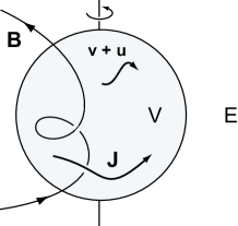
Figure 1: A dynamo in a volume $V$ that need not be spherical, with exterior vacuum $E$. The fluid in $V$ has a magnetic resistivity $\eta$, and the flow $V$ consists of a stationary component $v$ and the turbulent convection $u$, which may have an arbitrary distribution over spatial scales. The currents $J$ are restricted to $V$, and both currents and flows are tangential to the boundary $\partial V$. The magnetic field $B$ is continuous through $\partial V$.

Examples of such function sets are the free decay modes, or the eigenfunctions of a homogeneous spherical dynamo (see Ref. KR80 , Chap. 14). These two sets are actually self-adjoint so that the adjoint sets are obtained by complex conjugation: $\hat{\mbox{\boldmath$b$}}{}^{i}(\mbox{\boldmath$r$})=\mbox{\boldmath$b$}^{i*}(\mbox{\boldmath$r$})$. Usually the situation is more complicated, and we refer to Schrinner et al. SJSH08 for the construction of the adjoint set of the eigenfunctions of the dynamo equation. From that construction a number of properties emerge, such as $\hat{\mbox{\boldmath$\jmath$}}{}\equiv$ adjoint of $\nabla\times\mbox{\boldmath$b$}\equiv\nabla\times\hat{\mbox{\boldmath$b$}}{}$, i.e. the adjoint operation commutes with $\nabla$.

II.1 Biorthogonal sets in $V$

It is of course possible to define an inner product in $V$ alone, and to construct an adjoint set $\hat{\mbox{\boldmath$b$}}{}^{i}$ of $\mbox{\boldmath$b$}^{j}$ so that these are biorthogonal in $V$: $\int_{V}\hat{\mbox{\boldmath$b$}}{}^{i}\cdot\mbox{\boldmath$b$}^{j}\,{\rm d}^{3}\mbox{\boldmath$r$}\,=\,\delta^{ij}$. But as we shall see these sets are not very convenient. Fortunately, the boundary conditions permit construction of a very useful biorthogonal set in $V$, starting from sets $\{\hat{\mbox{\boldmath$b$}}{}^{i}\}$ and $\{\mbox{\boldmath$b$}^{j}\}$ that are biorthogonal in $V+E$. For two fields $\mbox{\boldmath$b$}_{1}$ and $\mbox{\boldmath$b$}_{2}$ with associated currents $\mbox{\boldmath$j$}=\nabla\times\mbox{\boldmath$b$}$ and vector potentials $a$, where $\nabla\times\mbox{\boldmath$a$}=\mbox{\boldmath$b$}$, we have $\nabla\cdot\hat{\mbox{\boldmath$b$}}{}_{1}\times\mbox{\boldmath$a$}_{2}=\hat{\mbox{\boldmath$\jmath$}}{}_{1}\cdot\mbox{\boldmath$a$}_{2}-\hat{\mbox{\boldmath$b$}}{}_{1}\cdot\mbox{\boldmath$b$}_{2}$, whence

$$\int_{V+E}\hat{\mbox{\boldmath$b$}}{}_{1}\cdot\mbox{\boldmath$b$}_{2}\,{\rm d}^{3}\mbox{\boldmath$r$} =$$

$$\int_{V}\hat{\mbox{\boldmath$\jmath$}}{}_{1}\cdot\mbox{\boldmath$a$}_{2}\,{\rm d}^{3}\mbox{\boldmath$r$} - \left(\oint_{\partial E}+\oint_{\partial V}\right)\hat{\mbox{\boldmath$b$}}{}_{1}\times\mbox{\boldmath$a$}_{2}\cdot{\rm d}^{2}\mbox{\boldmath$\sigma$}\ .\quad$$ (5)

Here $\partial V$ and $\partial E$ indicate the boundary of $V$ and $E$, respectively. The surface integrals cancel because the field is continuous through $\partial V$ and the vector potential can be constructed to be so. Volume integrals containing currents may be restricted to $V$ since $\mbox{\boldmath$j$}=0$ in $E$. This leads to:

$$\int_{V+E}\hat{\mbox{\boldmath$b$}}{}^{i}\cdot\mbox{\boldmath$b$}^{j}\,{\rm d}^{3}\mbox{\boldmath$r$} = \int_{V}\hat{\mbox{\boldmath$\jmath$}}{}^{i}\cdot\mbox{\boldmath$a$}^{j}\,{\rm d}^{3}\mbox{\boldmath$r$}$$ (6)

$$= \int_{V}\hat{\mbox{\boldmath$a$}}{}^{i}\cdot\mbox{\boldmath$j$}^{j}\,{\rm d}^{3}\mbox{\boldmath$r$}\,=\delta^{ij}\ .$$

These relations are invariant under a gauge transformation $\mbox{\boldmath$a$}\rightarrow\mbox{\boldmath$a$}+\nabla\psi$ because $\int_{V}\hat{\mbox{\boldmath$\jmath$}}{}\cdot\nabla\psi\,{\rm d}^{3}\mbox{\boldmath$r$}=\int_{V}\nabla\cdot(\psi\hat{\mbox{\boldmath$\jmath$}}{})\,{\rm d}^{3}\mbox{\boldmath$r$}=\int_{\partial V}\psi\,\hat{\mbox{\boldmath$\jmath$}}{}\cdot{\rm d}^{2}\mbox{\boldmath$\sigma$}=0$, as (adjoint) currents run parallel to the boundary. Currents and vector potentials thus form a biorthogonal set in $V$, and this is essential for our study.

II.2 Closure relations

Completeness means that any reasonable field $B$ should have a unique expansion (3). Completeness implies the existence of closure relations. The best known example is from quantum mechanics where orthonormality of two eigenstates $m$ and $n$ means that $\int\psi_{m}(\mbox{\boldmath$r$})^{*}\psi_{n}(\mbox{\boldmath$r$})\,{\rm d}^{3}\mbox{\boldmath$r$}=\delta_{mn}$, and the closure relation is $\sum_{n}\psi_{n}(\mbox{\boldmath$r$})^{*}\psi_{n}(\mbox{\boldmath$r$}^{\prime})=\delta(\mbox{\boldmath$r$}-\mbox{\boldmath$r$}^{\prime})$, provided the sum is over a complete set of eigenstates D78 . In the present context it can be shown that

$$\sum_{i}\,\hat{b}_{k2}^{i}\,b_{\ell 1}^{i}\,=\sum_{i}\,\hat{\jmath}{}_{k2}^{i}\,a_{\ell 1}^{i} = \sum_{i}\,\hat{a}_{k2}^{i}\,j_{\ell 1}^{i}$$ (7)

$$= \delta({\it 1}-{\it 2})\,\delta_{k\ell}\ .$$

Notation: $\it 1=\mbox{\boldmath$r$}_{1},\it 2=\mbox{\boldmath$r$}_{2}$, $b_{\ell 1}^{i}=\ell$-th vector component of $\mbox{\boldmath$b$}^{i}(\mbox{\boldmath$r$}_{1})$, etc. Relation (7) says that the expressions on the left are unit operators in the discrete and continuous indices. There are several other closure relations, and the one we actually need is

$$\sum_{i}\,\hat{\jmath}{}_{k2}^{i}\,b_{\ell 1}^{i}\,=\,\epsilon_{k\ell m}\,\delta({\it 1}-{\it 2})\nabla_{m2}\ .$$ (8)

Relations (7) and (8) hold under an integral sign $\int_{V}{\rm d}{\it 2}\cdots$ and are to be regarded as an operator acting on all $\mbox{\boldmath$r$}_{2}$ dependence in the integrand. Care is needed when applying these closure relations, and for details we refer the reader to Appendix C of Ref. HS95 . Recall that we have absorbed the factor $4\pi/c$ in the definition of the current.

III Mode equations

On taking the inner product of (3) with $\hat{\mbox{\boldmath$b$}}{}^{k}$ we obtain with the help of (4):

$$a^{k}(t)\,=\,\int_{V+E}\,\hat{\mbox{\boldmath$b$}}{}^{k}\cdot\mbox{\boldmath$B$}\;{\rm d}^{3}\mbox{\boldmath$r$}\ .$$ (9)

To obtain the evolution equation of $a^{k}$, we take the time derivative $\dot{{\ }}=\partial_{t}\/$ and split the integral in two parts:

$$\dot{a}^{k}(t)\,=\,\int_{V}\,\hat{\mbox{\boldmath$b$}}{}^{k}\cdot\dot{\mbox{\boldmath$B$}}\;{\rm d}^{3}\mbox{\boldmath$r$}\,+\,\int_{E}\,\hat{\mbox{\boldmath$b$}}{}^{k}\cdot\dot{\mbox{\boldmath$B$}}\;{\rm d}^{3}\mbox{\boldmath$r$}\ .$$ (10)

In the first term we may use the induction equation, but we have no equation for $\partial_{t}\mbox{\boldmath$B$}$ in $E$, where $B$ is simply the potential field continuation of $B$ on $\partial V$. Omitting the second term is no option as it amounts to saying that $\partial_{t}\mbox{\boldmath$B$}=0$ in $E$. A way out of this dilemma is to integrate the right hand side of (9) by parts, as in (5), to obtain ($\nabla\times\mbox{\boldmath$A$}=\mbox{\boldmath$B$}$):

$$a^{k}(t)\,=\,\int_{V}\,\hat{\mbox{\boldmath$\jmath$}}{}^{k}\cdot\mbox{\boldmath$A$}\;{\rm d}^{3}\mbox{\boldmath$r$}\ .$$ (11)

Derivation of the mode equations is now straightforward. Take the time derivative of (11) and insert the uncurled induction equation, $\partial_{t}\mbox{\boldmath$A$}=\{(\mbox{\boldmath$v$}+\mbox{\boldmath$u$})-\,\eta\nabla\}\times\mbox{\boldmath$B$}+\nabla\psi$, to obtain

$$\dot{a}^{k}(t)\,=\,\int_{V}\,\hat{\mbox{\boldmath$\jmath$}}{}^{k}\cdot\{(\mbox{\boldmath$v$}+\mbox{\boldmath$u$})-\,\eta\nabla\}\times\mbox{\boldmath$B$}\;{\rm d}^{3}\mbox{\boldmath$r$}\ .$$ (12)

The gradient term produces zero, see below (6). At this point we note that if we had used a biorthogonal set $\mbox{\boldmath$b$}^{i}(\mbox{\boldmath$r$}),\,\hat{\mbox{\boldmath$b$}}{}^{j}(\mbox{\boldmath$r$})$ in $V$, the dilemma mentioned a moment ago would not occur, because the integrals are restricted to $V$. However (12) would then read

$$\dot{a}^{k}(t)\,=\,\int_{V}\,\hat{\mbox{\boldmath$b$}}{}^{k}\cdot\nabla\times\{(\mbox{\boldmath$v$}+\mbox{\boldmath$u$})-\,\eta\nabla\}\times\mbox{\boldmath$B$}\;{\rm d}^{3}\mbox{\boldmath$r$}\ .$$ (13)

There is no conflict between (12) and (13) because they use different bases: biorthogonal in $V+E$ and biorthogonal in $V$, respectively. So $\hat{\mbox{\boldmath$b$}}{}^{k},\,\hat{\mbox{\boldmath$\jmath$}}{}^{k}$ in (12) are not the same as $\hat{\mbox{\boldmath$b$}}{}^{k},\,\hat{\mbox{\boldmath$\jmath$}}{}^{k}$ in (13)!

The extra $\nabla$ on the right hand side of (13) is very inconvenient and cannot be removed by integration by parts because the surface integral over $\partial V$ is nonzero (see Appendix A). It would stay with us and cause havoc in all subsequent analytical and numerical work. Therefore (12) is much to be preferred. This point was one of the main drivers for developing the formalism of the previous Section. Because of its importance, we discuss the issue in more detail in Appendix A.

On inserting $\mbox{\boldmath$B$}=\sum_{\ell}a^{\ell}\,\mbox{\boldmath$b$}^{\ell}$ in (12), we arrive at the mode equations

$$\dot{a}^{k} = \sum_{\ell}\,\{S^{k\ell}+C^{k\ell}(t)\}\,a^{\ell}\ ,$$ (14)

$$\rm with$$

$$S^{k\ell} = \int_{V}\;\hat{\mbox{\boldmath$\jmath$}}{}^{k}\cdot(\mbox{\boldmath$v$}-\,\eta\nabla\,)\times\mbox{\boldmath$b$}^{\ell}\;{\rm d}^{3}\mbox{\boldmath$r$}\ ;\qquad\qquad$$ (15)

$$C^{k\ell}(t) = \int_{V}\;\hat{\mbox{\boldmath$\jmath$}}{}^{k}\cdot\mbox{\boldmath$u$}\times\mbox{\boldmath$b$}^{\ell}\;{\rm d}^{3}\mbox{\boldmath$r$}$$

$$= -\int_{V}\;\mbox{\boldmath$u$}\cdot\hat{\mbox{\boldmath$\jmath$}}{}^{k}\times\mbox{\boldmath$b$}^{\ell}\;{\rm d}^{3}\mbox{\boldmath$r$}\ .$$

The base functions that occur in the definition of the matrix elements $S^{k\ell}$ and $C^{k\ell}$ may be thought of as spatial filters with positive and negative signs indicating how the velocities $v$ and $u$ are to be weighted in the volume integration over $V$. The boundary conditions make that the integrals are of the type $\langle{\rm current}|{\rm operator}|{\rm field}\rangle$ rather than $\langle{\rm field}|{\rm operator}|{\rm field}\rangle$. The boundary conditions have therefore a profound effect on the definition of these filters. Mode equations of the type (14) had already been derived by Elsasser E46 , although he considered steady flows only. Compared to the time scales in the steady matrix $S^{k\ell}$, the elements $C^{k\ell}$ fluctuate rapidly because $\mbox{\boldmath$u$}(\mbox{\boldmath$r$},t)$ does. The mode equations are therefore stochastic equations, and we shall use the theory of these equations to infer averages of the mode coefficients.

IV Stochastic equations with multiplicative noise

Consider a linear equation of the type

$$\frac{\partial x}{\partial t}\,=\,\{A+F(t)\}x\ ,$$ (17)

where linear means linear in $x$. The quantity $x$ may be anything, a scalar, a vector such as $B$, or other. The operator $A$ is independent of time but $F(t)$ fluctuates randomly, with a correlation time $\tau_{\rm c}$ and zero mean, $\langle F\rangle\,=\,0$. This ‘noise term’ $F(t)$ is said to be multiplicative as it multiplies the independent variable $x$, and that makes (17) more complicated than for example $\partial x/\partial t\,=\,Ax+F(t)$, where the noise term is additive.

A tenet of the theory of stochastic differential equations is that the average $\langle x\rangle$ obeys a closed equation vK76 :

$$\frac{\partial}{\partial t}\,\langle x\rangle = \biggl{\{}A\,+\int_{0}^{\infty}{\rm d}\tau\,\langle F(t)\exp(A\tau)\cdot\qquad\qquad$$ (18)

$$\qquad\qquad\cdot\,F(t-\tau)\rangle\exp(-A\tau)\biggr{\}}\langle x\rangle\ ,$$

The right hand side of (18) is actually the first term of a series with terms of order $(F\tau_{\rm c})^{n}$ containing higher-than-second-order correlation functions vK74 . Here $F$ stands for $F_{\rm r.m.s.}$. We assume that the correlation time is small, $F\tau_{\rm c}\ll 1$, so that only the first term survives and only second order correlations matter, as in (18). Frequently also $A\tau_{\rm c}\ll 1$ holds, and then we may ignore the exponential operators in (18). These evolution operators $\exp(\pm A\tau)$, incidentally, ensure that the transport coefficients for $\langle x\rangle$ derived from (18) are Galilean invariant H03 . Relation (18) will be applied several times in what follows.

V The average mode coefficients

The equation for the average $\langle a^{k}\rangle$ is in principle available in the literature, but hidden in two papers H88 ; HS95 . We summarise the derivation here, and apply (18) to (14):

$$\frac{{\rm d}}{{\rm d}t}\,\langle a^{k}\rangle\,=\,\left\{\,S^{k\ell}\,+\,\int_{0}^{\infty}\!{\rm d}\tau\,\langle C^{ki}(t)C^{i\ell}(t-\tau)\rangle\,\right\}\langle a^{\ell}\rangle\ .$$ (19)

Summation over double upper indices (here $i$ and $\ell$) is implied. Before we elaborate the correlation function we verify the conditions to be satisfied:

(1) $C^{k\ell}\tau_{\rm c}\ll 1$, the usual condition of a short correlation time, now in the context of the present application [ $C^{k\ell}$ is understood to indicate a characteristic magnitude ]. We estimate the value of $C^{k\ell}\tau_{\rm c}$ for the geodynamo. The volume integration in (LABEL:eq:ckl) reduces $u$ effectively to $u_{\rm r.m.s.}N^{-1/2}$ where $N\sim 4R^{3}/\lambda_{\rm c}^{3}\sim$ number of convection cells; $R$ is the radius of the outer core, and $\lambda_{\rm c}$ the correlation length (the volume of the inner core is negligible). We estimate $\hat{\mbox{\boldmath$\jmath$}}{}^{k}=\nabla\times\hat{\mbox{\boldmath$b$}}{}^{k}\sim\hat{b}^{k}/(R/k)$ and $\int_{V}\hat{b}^{k}\,b^{\ell}{\rm d}^{3}\mbox{\boldmath$r$}=O(1)$, and $u_{\rm r.m.s.}\tau_{\rm c}\sim\lambda_{\rm c}$. This leads to

$$C^{k\ell}\tau_{\rm c} \sim u_{\rm r.m.s.}\,\tau_{\rm c}\left(\frac{4R^{3}}{\lambda_{\rm c}^{3}}\right)^{-1/2}\!\!\int_{V}\frac{\hat{b}^{k}\,b^{\ell}}{R/k}\;{\rm d}^{3}\mbox{\boldmath$r$}$$ (20)

$$\sim \frac{k}{2}\;\left(\frac{\lambda_{\rm c}}{R}\right)^{5/2}\ .$$

For the geodynamo we have $R/\lambda_{\rm c}\sim 3.5$. It follows that $C^{k\ell}\tau_{\rm c}\,\sim\,0.02k$ so that $C^{k\ell}\tau_{\rm c}\ll 1$ seems well satisfied for the lowest multipole coefficients $a^{k}$ (even though $u_{\rm r.m.s.}\tau_{\rm c}\sim\lambda_{\rm c}\,$!). There is an interesting connection here with the problem of the First Order Smoothing Approximation (FOSA) in mean field theory, and we refer to Sec. VIII where we illustrate how this FOSA problem seems to be partially eliminated.

(2) $S^{k\ell}\tau_{\rm c}\ll 1$. The magnitude of $S^{k\ell}$ is set by the resistive term in (15), and in much the same way we obtain

$$S^{k\ell}\tau_{\rm c}\,\sim\,k\ell\,\eta\tau_{\rm c}/R^{2}\ .$$ (21)

For the geodynamo we have $\eta\sim 1\,$m${}^{2}\,$s^-1, and $S^{k\ell}\tau_{\rm c}\,\sim\,3\cdot 10^{-4}k\ell$ so that $S^{k\ell}\tau_{\rm c}\ll 1$ holds except for high order modes. We have to assume therefore that these modes contribute little, which is plausible because they will have small amplitudes.

The correlation function in (19) is evaluated in Appendix B, and as a result we may write (19) as follows:

$$\frac{{\rm d}}{{\rm d}t}\,\langle a^{k}\rangle\,=\,D^{k\ell}\langle a^{\ell}\rangle\ ,$$ (22)

with

$$D^{k\ell}\,=\,\int_{V}\;\hat{\mbox{\boldmath$\jmath$}}{}^{k}\cdot D\mbox{\boldmath$b$}^{\ell}\;{\rm d}^{3}\mbox{\boldmath$r$}\ ,$$ (23)

where the operator $D$ is defined as

$$D\mbox{\boldmath$b$}\,=\,\mbox{\boldmath$v$}\times\mbox{\boldmath$b$}+\mbox{\boldmath$\alpha$}\cdot\mbox{\boldmath$b$}-\mbox{\boldmath$\beta$}:(\nabla\mbox{\boldmath$b$})-\eta\nabla\times\mbox{\boldmath$b$}\ .$$ (24)

Notation: $(\mbox{\boldmath$\alpha$}\cdot\mbox{\boldmath$b$})_{i}=\alpha_{ik}b_{k}$ and $[\mbox{\boldmath$\beta$}:(\nabla\mbox{\boldmath$b$})]_{i}=\beta_{ik\ell}(\nabla_{k}b_{\ell})$. The operator $D$ is intimately related to the dynamo equation, which reads (Appendix B):

$$\frac{\partial}{\partial t}\,\langle\mbox{\boldmath$B$}\rangle\,=\,\nabla\times D\langle\mbox{\boldmath$B$}\rangle\ .$$ (25)

The fact that the operator of the dynamo equation for the mean field emerges in (22) is quite independent of which set of base functions is used. At this point we see how mean field theory emerges as we study the statistical properties of the mean mode coefficients. It happens because we take averages, and since the simplest averages over the turbulent convection involve $\mbox{\boldmath$v$},\,\mbox{\boldmath$\alpha$}$ and $\beta$, it is perhaps not surprising that the operator of the dynamo equation for the mean field appears. But we use the mean field $\langle\mbox{\boldmath$B$}\rangle$ as a mathematical concept only, without much of a physical meaning attached to it.

V.1 Dynamo action and dynamo equation

The fact that the dynamo equation for the mean emerges as we set up the theory indicates a deep connection between dynamo action in flows with a random element and the mean-field dynamo equation. What this relation is can be seen by adopting the eigenfunctions of the dynamo equation as the complete function set $\{\mbox{\boldmath$b$}^{i}\}$, with eigenvalues $\lambda_{i}$ lowind . Then we have

$$\nabla\times D\mbox{\boldmath$b$}^{i}\,=\,\lambda_{i}\,\mbox{\boldmath$b$}^{i}\ .$$ (26)

Relations (26) through (29) below hold only if we use the eigenfunctions of the dynamo equation as our function set. Schrinner et al. SJSH08 show how these eigenfunctions and their adjoints may be constructed.

The computation of $D^{k\ell}$ from (23) has several potential pitfalls. Integration by parts to $\int_{V}\hat{\mbox{\boldmath$b$}}{}^{k}\cdot\nabla\times D\mbox{\boldmath$b$}^{\ell}\,{\rm d}^{3}\mbox{\boldmath$r$}$, with hopes of using (26), is not possible because the surface term $\oint_{\partial V}\hat{\mbox{\boldmath$b$}}{}^{k}\times D\mbox{\boldmath$b$}^{\ell}\cdot{\rm d}^{2}\mbox{\boldmath$\sigma$}$ does not vanish. And to argue that (23) $=\int_{V+E}\,\hat{\mbox{\boldmath$\jmath$}}{}^{k}\cdot D\mbox{\boldmath$b$}^{\ell}\,{\rm d}^{3}\mbox{\boldmath$r$}=\int_{V+E}\,\hat{\mbox{\boldmath$b$}}{}^{k}\cdot\nabla\times D\mbox{\boldmath$b$}^{\ell}\,{\rm d}^{3}\mbox{\boldmath$r$}$ does not work either because $D$ is not defined in $E$. A safe way is to uncurl (26) to $D\mbox{\boldmath$b$}^{i}\,=\,\lambda_{i}\,\mbox{\boldmath$a$}^{i}+\nabla\phi$, and to insert that in (23):

$$D^{k\ell}\,=\,\lambda_{\ell}\int_{V}\;\hat{\mbox{\boldmath$\jmath$}}{}^{k}\cdot\mbox{\boldmath$a$}^{\ell}\;{\rm d}^{3}\mbox{\boldmath$r$}\,=\,\lambda_{\ell}\,\delta^{k\ell}\ .$$ (27)

The gradient term produces zero, see below (6). The detour via the vector potential in (27) allows us to avoid trouble due to the discontinuity of the operator $D$ on $\partial V$.

Returning to the evolution of the mean mode coefficients, we now have

$$\frac{{\rm d}}{{\rm d}t}\,\langle a^{k}\rangle\,=\,\lambda_{k}\langle a^{k}\rangle\ ,\quad{\rm or}\quad\langle a^{k}\rangle\,\propto\,\exp(\lambda_{k}t)\ .$$ (28)

If we choose the eigenfunctions of the dynamo equation (the operator $\nabla\times D$) as a basis to represent the magnetic field, then the mean mode coefficients decay as simple exponentials at a rate set by the eigenvalue of the mode. Representation of the field $B$ of the dynamo in terms of the eigenfunctions of its dynamo equations is therefore an efficient way to expose the underlying physics. The autocorrelation of the expansion coefficients becomes:

$$\langle a^{k}(t+\tau)a^{k*}(t)\rangle\,=\,\langle|a^{k}|^{2}\rangle\cdot\exp(\lambda_{k}\tau)$$ (29)

(no summation over $k$). The proof is simple and not given here. The mean squares of the expansion coefficients are computed in Sec. VII, relation (40).

Of course one may always use a different representation. In that case $D^{k\ell}$ is no longer diagonal and the mean mode coefficients have a more complicated time dependence. Equation (22) may be integrated to

$$\langle a^{k}\rangle|_{t}\,=\,[\exp(Dt)]^{k\ell}\,\langle a^{\ell}\rangle|_{t=0}\ .$$ (30)

The time dependence of $\langle a^{k}\rangle|_{t}$ and the autocorrelation function is now a mixture of exponentials.

V.2 Absence of growing modes

For the theory developed here to make sense it is necessary that all eigenvalues have a negative real part, $\Re\lambda_{k}<0$, and we shall assume that this is the case. The implication is that if we measure the flow in a dynamo(model) with all feedbacks of the Lorentz force acting on it, we should find, on solving (26) with $\alpha_{ij}$ and $\beta_{ijk}$ and mean flow computed from these measurements, that all eigenvalues have $\Re\lambda_{k}<0$. This is one of the checks on a correct determination of the dynamo coefficients. Of course this can only be true if we restrict ourselves to kinematically stable dynamos (see Sec. I for a definition). A proof that $\Re\lambda_{k}<0$ has been given for a few special cases with infinite conductivity H87 ; vGH89 , but a general proof is lacking. In Appendix C we push the issue one step forward and prove that all eigenvalues of the dynamo equation of a statistically steady dynamo with locally isotropic turbulence and finite conductivity have negative real parts.

A consequence is that all mean mode coefficients approach zero, $\langle a^{k}\rangle\downarrow 0$ and that the mean field $\langle\mbox{\boldmath$B$}\rangle=\sum_{i}\langle a^{i}\rangle\mbox{\boldmath$b$}^{i}$ will also be zero,

$$\langle\mbox{\boldmath$B$}\rangle=0\ .$$ (31)

Ultimately, this may be seen as a consequence of the fact that both $B$ and $-\mbox{\boldmath$B$}$ are solutions of the MHD equations for given $V$ and since there is always a (possibly very small) transition probability between the two states, a full ensemble average $\langle\mbox{\boldmath$B$}\rangle$ of a statistically steady dynamo will be zero. This is also true if $\langle\cdot\rangle$ is a time average, provided the average is over a sufficiently long time, so that all dynamical states of the system are sampled. For the geodynamo that would mean an average over a time interval containing a large number of reversals (or cycle periods in case of the solar dynamo).

From a practical point of view, it is therefore not obvious what a time- or an ensemble-averaged field $\langle\mbox{\boldmath$B$}\rangle$ is telling us about the actual field $B$ of a dynamo, and this is one of the main motivations for the approach presented in this paper. A similar objection may be held against the mean mode coefficients $\langle a^{k}\rangle$. They also do not contain much information since they are zero (after some time), but they are indispensable for setting up the theory. The cross correlation coefficients $\langle a^{k}a^{\ell}\rangle$ that we compute in the next Section are much more useful in this regard.

V.3 Mode excitation and phase mixing

The interpretation of these results is the following H03 . The eigenmodes of the dynamo equation serve as a kind of normal modes of the dynamo. These normal modes are transiently excited and have a frequency $\Im\lambda_{k}$. The relative r.m.s. mode amplitudes will be computed in the next Section. Random phase shifts due to the stochastic forcing render the modes quasi-periodic with a coherence time $-1/\Re\lambda_{k}$. Due to the averaging, these phase shifts appear as a damping of the mean mode amplitude $\langle a^{k}\rangle$. This is a familiar phenomenon in statistical physics known as phase mixing.

VI Mean square mode coefficients

In this Section we are interested in the cross-correlation coefficients $\langle a^{k}a^{\ell*}\rangle$. The strategy is to derive an equation of the type $({\rm d}/{\rm d}t)\{a^{k}a^{\ell*}\}={\rm operator}\cdot\{a^{i}a^{j*}\}$. We may then apply relation (18) to find the equation for $\langle a^{k}a^{\ell*}\rangle$ (see Ref. vK76 , § 16). The analysis is straightforward (we use $\dot{\ }={\rm d}/{\rm d}t\,)$:

$$(a^{k}a^{\ell*})\dot{\ } = \dot{a}^{k}a^{\ell*}\,+\,a^{k}\dot{a}^{\ell*}$$ (32)

$$= \left(S^{ki}+C^{ki}\right)a^{i}a^{\ell*}\,+\,a^{k}\left(S^{\ell j*}+C^{\ell j*}\right)a^{j*}$$

$$= \mbox{\LARGE(}\underbrace{S^{ki}\delta^{\ell j}\,+\,S^{\ell j*}\delta^{ki}}_{A}$$

$$\qquad\quad+\,\,\underbrace{C^{ki}\delta^{\ell j}\,+\,C^{\ell j*}\delta^{ki}}_{F(t)}\mbox{\LARGE)}\;a^{i}a^{j*}\ .$$

This is of the form (17) with $x=\{a^{k}a^{\ell*}\}$. The conditions of a short correlation time $F\tau_{\rm c}\ll 1$ and $A\tau_{\rm c}\ll 1$ are the same as (20) and (21), respectively. The application of recipe (18) for the average is mainly a matter of bookkeeping of upper indices:

$$\frac{{\rm d}}{{\rm d}t}\,\bigl{\langle}a^{k}a^{\ell*}\bigr{\rangle} = \biggl{\{}S^{km}\delta^{\ell n}\,+\,S^{\ell n*}\delta^{km}\,+\int_{0}^{\infty}\!{\rm d}\tau\;\Big{\langle}\Big{(}C^{ki}(t)\,\delta^{\ell j}+C^{\ell j*}(t)\,\delta^{ki}\Big{)}\cdot$$ (33)

$$\qquad\qquad\qquad\qquad\qquad\qquad\qquad\cdot\,\Big{(}C^{im}(t-\tau)\,\delta^{jn}+C^{jn*}(t-\tau)\,\delta^{im}\Big{)}\Big{\rangle}\biggr{\}}\,\bigl{\langle}a^{m}a^{n*}\bigr{\rangle}$$

$$= \biggl{\{}S^{km}\delta^{\ell n}\,+\,S^{\ell n*}\delta^{km}\,+\int_{0}^{\infty}\!{\rm d}\tau\;\Big{(}\bigl{\langle}C(t)\cdot C(t-\tau)\bigr{\rangle}^{km}\,\delta^{\ell n}\,+\,\bigl{\langle}C(t)\cdot C(t-\tau)\bigr{\rangle}^{\ell n*}\,\delta^{km}\Big{)}$$

$$\qquad\qquad\qquad\qquad\qquad+\int_{0}^{\infty}\!{\rm d}\tau\;\Big{(}\bigl{\langle}C^{km}(t)C^{\ell n*}(t-\tau)\bigr{\rangle}\,+\,\bigl{\langle}C^{\ell n*}(t)C^{km}(t-\tau)\bigr{\rangle}\Big{)}\biggr{\}}\,\bigl{\langle}a^{m}a^{n*}\bigr{\rangle}\qquad$$

$$= \biggl{\{}D^{km}\delta^{\ell n}\,+\,D^{\ell n*}\delta^{km}\,+\int_{0}^{\infty}\!{\rm d}\tau\;\Big{(}\bigl{\langle}C^{km}(t)C^{\ell n*}(t-\tau)\bigr{\rangle}\,+\,\bigl{\langle}C^{\ell n*}(t)C^{km}(t-\tau)\bigr{\rangle}\Big{)}\biggr{\}}\,\bigl{\langle}a^{m}a^{n*}\bigr{\rangle}\ .$$

We see that the dynamo operator $D$ also plays a role in the evolution of the mean square mode coefficients. Relation (33) becomes more transparent if we adopt the eigenfunctions of $\nabla\times D$ as our basis:

$$\biggl{(}\frac{{\rm d}}{{\rm d}t}\,-\,\lambda_{k} - \lambda_{\ell}^{*}\biggr{)}\langle a^{k}a^{\ell*}\rangle\,=\qquad\qquad\qquad\qquad\qquad$$ (34)

$$\quad\left(M^{km\ell n}+M^{\ell nkm*}\right)\langle a^{m}a^{n*}\rangle\ .$$

(summation over $n,m$, not over $k,\ell$). The matrix $M^{km\ell n}$ is defined as

$$M^{km\ell n}\,=\,\int_{0}^{\infty}\!{\rm d}\tau\,\langle C^{km}(t)C^{\ell n*}(t-\tau)\rangle\ .$$ (35)

VI.1 Interpretation of Eq. (34)

Equation (34) describes the time evolution of the mean square mode coefficients $\langle a^{k}a^{\ell*}\rangle$. We replace ${\rm d}/{\rm d}t$ by $\Lambda$, as usual, to obtain the eigenvalue problem (the double indices $k,\ell$ and $m,n$ may each be grouped into a single new index). Of interest is the largest eigenvalue $\Lambda$, which should be approximately zero, otherwise $\langle a^{k}a^{\ell*}\rangle$ would either grow indefinitely, or become zero. This is again a matter of using the correct values of the dynamo coefficients. For instance, in a statistically steady geodynamo simulation the magnetic energy is on average constant, which implies that the mean square mode coefficients $\langle a^{k}a^{\ell*}\rangle$ are constant, even though some of the modes may be quasi-periodic. A determination of the dynamo coefficients $\alpha_{ij}$ and $\beta_{ijk}$ from a measurement of velocity correlation functions in this dynamo must then result in Eq. (34) having a stationary solution. This solution is the eigenvector belonging to the eigenvalue $\Lambda=0$ and it specifies the relative magnitudes of the correlation coefficients $\langle a^{k}a^{\ell*}\rangle$ (the absolute level is out of reach and requires explicit inclusion of nonlinear effects). These contain a lot of information, such as the distribution of magnetic energy over spatial scales. All other eigenvalues $\Lambda$ should have negative real parts, and correspond to transient initial states.

VI.2 Computation of $M^{km\ell n}$

Expression (35) for $M^{km\ell n}$ looks very similar to the correlation function in (19), but there is an important difference: there is no internal summation over modes. The closure relation is therefore no longer a comrade in arms, which renders evaluation of (35) much less straightforward. We insert (LABEL:eq:ckl) in (35):

$$M^{km\ell n} = \int_{0}^{\infty}\!{\rm d}\tau\,\langle C^{km}(t)C^{\ell n*}(t-\tau)\rangle$$ (36)

$$= \int\!\!\int_{V}{\rm d}{\it 1}{\rm d}{\it 2}\;(\hat{\mbox{\boldmath$\jmath$}}{}^{k}\times\mbox{\boldmath$b$}^{m})_{p1}\,(\hat{\mbox{\boldmath$\jmath$}}{}^{\ell}\times\mbox{\boldmath$b$}^{n})_{q2}^{*}\cdot\qquad$$

$$\qquad\qquad\qquad\quad\cdot\,\int_{0}^{\infty}\!{\rm d}\tau\,\langle u_{p1}^{t}u_{q2}^{t-\tau}\rangle\ .$$

Here ${\it 1}=\mbox{\boldmath$r$}_{1}$, ${\it 2}=\mbox{\boldmath$r$}_{2}$, index $p1$ indicates $p$-th vector component at position $\mbox{\boldmath$r$}_{1}$, $u_{p1}^{t}=p$-th vector component of $u$ at position $\mbox{\boldmath$r$}_{1}$ and time $t$, etc. Summation over the vector indices $p,q$ is implied.

There is an opportunity to simplify relation (36) if the correlation length $\lambda_{\rm c}$ of the flow $u$ is much smaller than the size of the dynamo – in other words, if there is a separation of spatial scales. In that case we put $\mbox{\boldmath$r$}_{2}=\mbox{\boldmath$r$}_{1}+\mbox{\boldmath$\rho$}$ and note that $\langle u_{p1}^{t}u_{q2}^{t-\tau}\rangle$ is zero if $\rho\geq\lambda_{\rm c}$. Since $\hat{\mbox{\boldmath$\jmath$}}{}^{k}\times\mbox{\boldmath$b$}^{m}$ and $\hat{\mbox{\boldmath$\jmath$}}{}^{\ell}\times\mbox{\boldmath$b$}^{n}$ are both of much larger spatial scale ($\sim$ size dynamo), they are, from their point of view, either evaluated at virtually the same location or the correlation function is zero. It follows that

$$M^{km\ell n}\,\simeq\,\int_{V}{\rm d}^{3}\mbox{\boldmath$r$}\;(\hat{\mbox{\boldmath$\jmath$}}{}^{k}\times\mbox{\boldmath$b$}^{m})_{p}\,(\hat{\mbox{\boldmath$\jmath$}}{}^{\ell}\times\mbox{\boldmath$b$}^{n})_{q}^{*}\;\sigma_{pq}(\mbox{\boldmath$r$})\ ,$$ (37)

where the tensor $\sigma_{pq}$ is given by

$$\sigma_{pq}(\mbox{\boldmath$r$})\,=\,\int_{V}{\rm d}^{3}\mbox{\boldmath$\rho$}\int_{0}^{\infty}\!{\rm d}\tau\,\langle u_{p}(\mbox{\boldmath$r$},t)\,u_{q}(\mbox{\boldmath$r$}+\mbox{\boldmath$\rho$},t-\tau)\rangle\ .$$ (38)

The integration over $\rho$ extends over a small radius $\rho\sim\lambda_{\rm c}\ll$ size dynamo, centred on $r$. Relations (37) and (38) are a useful starting point for model dynamos with small scale turbulence, and we refer to Appendix C for an application. But often, for example in numerical geodynamo models, there is no separation of spatial scales. The theory developed here remains valid, but the only option for computing $M^{km\ell n}$ seems to be through measurements of the turbulent flow $u$. These permit computation of time series $C^{km}(t)$ from the definition (LABEL:eq:ckl), after which $M^{km\ell n}$ may be found as an integral over the cross correlation function $\langle C^{km}(t)C^{\ell n*}(t-\tau)\rangle$.

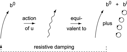
Figure 2: Intuitive picture of excitation of overtones in case of a dominant fundamental mode.

VII Mean overtone excitation level

The idea of determining mean square mode coefficients $\langle a^{k}a^{\ell*}\rangle$ of a statistically steady dynamo by solving the eigenvalue problem corresponding to Eq. (34) may be conceptually helpful, but in practice it leads to an extremely complicated problem because there are so many indices: each single index in Eq. (34) actually comprises three other indices corresponding to the three spatial degrees of freedom. Approximation methods seem to be the only way out. For example, if the geodynamo has a dominant dipole mode we may hope that the sums on the right hand side of (34) are dominated by the term $m=n=0$. Assuming a statistically steady state we then arrive at

$$\langle a^{k}a^{\ell*}\rangle\,\simeq\;-\;\frac{M^{k0\ell 0}+M^{\ell 0k0*}}{\lambda_{k}\,+\,\lambda_{\ell}^{*}}\;\langle|a^{0}|^{2}\rangle\ .$$ (39)

This relation gives the magnitude of the cross correlation $\langle a^{k}a^{\ell*}\rangle$ relative to the mean square amplitude of the fundamental mode. The mean square overtone amplitude is:

$$\langle|a^{k}|^{2}\rangle\,\simeq\;\frac{M^{k0k0}}{-\,\Re\lambda_{k}}\;\langle|a^{0}|^{2}\rangle\ .\vspace{2.mm}$$ (40)

Since $M^{k0k0}=\int_{0}^{\infty}\!{\rm d}\tau\,\langle C^{k0}(t)C^{k0*}(t-\tau)\rangle\simeq|C^{k0}|_{\rm r.m.s.}^{2}\tau_{\rm c}\allowbreak=\big{|}\int_{V}\,\mbox{\boldmath$u$}\cdot\hat{\mbox{\boldmath$\jmath$}}{}^{k}\times\mbox{\boldmath$b$}^{0}\,{\rm d}^{3}\mbox{\boldmath$r$}\big{|}_{\rm r.m.s.}^{2}\tau_{\rm c}\$ we obtain

$$\frac{\langle|a^{k}|^{2}\rangle}{\langle|a^{0}|^{2}\rangle}\;\simeq\;\frac{-1}{\Re\lambda_{k}}\;\left|\int_{V}\,\mbox{\boldmath$u$}\cdot\hat{\mbox{\boldmath$\jmath$}}{}^{k}\times\mbox{\boldmath$b$}^{0}\,{\rm d}^{3}\mbox{\boldmath$r$}\,\right|_{\rm r.m.s.}^{2}\tau_{\rm c}\vspace{2.mm}$$ (41)

The physical picture behind (41) is as follows, see Fig. 2. The turbulent convection $u$ creates new small scale fields (overtones) by continuously deforming the dominant fundamental mode. This is encoded in the numerator of (41). These overtones are subsequently damped by resistive effects ($\Re\lambda_{k}$ in the denominator). The balance of the two processes determines the excitation level. Excitation of overtone $k$ is effective at locations where $\hat{\mbox{\boldmath$\jmath$}}{}^{k}\times\mbox{\boldmath$b$}^{0}$ is large, in particular when the turbulent flow $u$ is parallel to it. Hoyng and Van Geffen HvG93 have derived a relation similar to (41) for a simple dynamo, and these authors found that it agrees accurately with numerical results.

Further progress requires evaluation of (41) or of $M^{k0k0}$, for which there are basically two options. For a model dynamo it may be done analytically. Otherwise we need to measure the flow $u$ and compute (41) as an integral over the correlation function of $C^{k0}(t)$.

Here we shall restrict ourselves to an estimate of the order of magnitude of (41) for a spherical dynamo with radius $R$. The volume integration in (41) may be estimated as in (20), except that we now do not eliminate the number of convective cells $N$:

$$C^{k0} \sim \int_{V}\,\mbox{\boldmath$u$}\cdot\hat{\mbox{\boldmath$\jmath$}}{}^{k}\times\mbox{\boldmath$b$}^{0}\,{\rm d}^{3}\mbox{\boldmath$r$}\;$$ (42)

$$\sim u_{\rm r.m.s.}\,N^{-1/2}\,(R/k)^{-1}\ ,$$

so that $|\int\cdots|_{\rm r.m.s.}^{2}\tau_{\rm c}\sim u_{\rm r.m.s.}^{2}\tau_{\rm c}\,N^{-1}(k/R)^{2}\sim(\beta/R^{2})\,N^{-1}k^{2}$, where $\beta$ is the turbulent diffusion coefficient. Due to the resistive term in (15), $\Re\lambda_{k}$ scales approximately as $k^{2}$, so that $k^{2}/(-\Re\lambda_{k})\sim$ constant $\sim R^{2}/\beta$. Hence we predict that to order of magnitude

$$\frac{\langle|a^{k}|^{2}\rangle}{\langle|a^{0}|^{2}\rangle}\;\sim\;\frac{\beta}{R^{2}}\;\frac{1}{N}\;\frac{k^{2}}{-\Re\lambda_{k}}\,\sim\,\frac{1}{N}\ \ \ \ {\rm for}\ \ \ \ k\ll\frac{R}{\lambda_{\rm c}}\ .$$ (43)

The meaning of $k$ above and in (20) and (21) is not immediately clear as it comprises three quantum numbers $n$ (radial) and $\ell,\,m$ for the two angular co-ordinates. Since $k$ appears when $R/k$ is taken to be the spatial scale of $\mbox{\boldmath$b$}^{k}$, one should assign $k=1$ to the fundamental mode. For overtones one may think of $k$ as a geometrical mean, $k=(n\ell m)^{1/3}$, but an exact interpretation is of course not possible.

The implication for the geodynamo is that the r.m.s. mode amplitude relative to the fundamental mode would be of the order of $N^{-1/2}\sim 0.1$, approximately independent of mode number. This does not seem to be an outrageous number, but it cannot be readily compared with the data MMM96 because these do not distinguish between modes of different radial order.

Estimate (43) assumes effectively that $k\ll R/\lambda_{\rm c}$, i.e. that $R/k$, the spatial scale of mode $\mbox{\boldmath$b$}^{k}$, is much larger than the correlation length $\lambda_{\rm c}$. For high-order overtones with $k\gg R/\lambda_{\rm c}$ (spatial scale of mode $\mbox{\boldmath$b$}^{k}$ smaller than $\lambda_{\rm c}$) we obtain:

$$\frac{\langle|a^{k}|^{2}\rangle}{\langle|a^{0}|^{2}\rangle}\;\sim\;\frac{1}{N}\;\left(\frac{R}{k\lambda_{\rm c}}\right)^{3}\,\qquad{\rm for}\qquad k\gg\,\frac{R}{\lambda_{\rm c}}\ .$$ (44)

For very high order modes the excitation level approaches zero.

VIII Discussion

We have analysed the statistical properties of the magnetic field generated by a turbulent dynamo in a nonlinearly saturated state. The properties of the mean and convective flow in this saturated state are supposed to be given, which allows us to use linear theory. Starting from an expansion in a set of base functions, we have derived statistical properties of the expansion coefficients $a^{k}(t)$, viz. the means $\langle a^{k}\rangle$, the cross correlations $\langle a^{k}a^{\ell*}\rangle$, and the autocorrelation functions $\langle a^{k}(t)a^{k*}(t+\tau)\rangle$. The convection may have any spatial scale distribution. Conditions for validity are (1) a short correlation time, $C^{k\ell}\tau_{\rm c}\ll 1$, and (2) the effect of the mean flow $v$ in one correlation time is small, $S^{k\ell}\tau_{\rm c}\ll 1$. The second assumption is made for convenience, and the theory can still be deployed if it does not hold. These two conditions have been worked out for the geodynamo in (20) and (21), and seem to be well satisfied for the lower multipole coefficients $a^{k}$. The two main tools enabling our analysis are (1) the fact that currents and vector potentials form a biorthogonal set in the volume $V$ of the dynamo, and (2) the theory of stochastic differential equations.

Any set of magnetic fields $\mbox{\boldmath$b$}^{k}(\mbox{\boldmath$r$})$ may be used for the expansion. However, since the theoretical results contain averages over the turbulence that also occur in mean field theory, it turns out that the eigenfunctions of the dynamo equation are a preferred set, in terms of which our results assume their simplest form. This is an important point, and the reader might easily get the wrong impression, as we pay quite some attention to the dynamo coefficients $\alpha_{ij}$ and $\beta_{ijk}$ and to eigenfunctions and eigenvalues of the dynamo equation. But this is only done in the interest of determining the preferred basis and its properties, not because we want to focus our study on the mean field concept $\langle\mbox{\boldmath$B$}\rangle$.

VIII.1 Nature of the dynamo field

The physical picture that emerges from our study is that the dynamo field is a superposition of transiently excited eigenmodes whose coherence time and frequency are determined by the corresponding eigenvalue of the dynamo equation, as had been surmised by Hoyng H03 . For the theory to make sense, all these eigenvalues should have negative real parts. This property could be proven in the restricted case of locally isotropic turbulence, but a general proof is still lacking. The r.m.s. excitation level of the modes is given by an equation that determines the cross correlations $\langle a^{k}a^{\ell*}\rangle$ up to an overall constant. It follows that the relative excitation level of the modes is determined by the statistics of the flow and by linear theory. This is an example showing that linear theory is not yet fully exhausted. Determination of the absolute excitation levels requires explicit inclusion of nonlinear effects in the theory. Unfortunately, this equation for $\langle a^{k}a^{\ell*}\rangle$ is rather complicated and cannot be solved in general. An approximate expression for $\langle|a^{k}|^{2}\rangle\,/\,\langle|a^{0}|^{2}\rangle$ exists when the fundamental mode is dominant in magnitude, which may hopefully apply in the case of numerical geodynamo models.

VIII.2 Applications

Application of this work is restricted to kinematically stable dynamos, as defined in Sec. I, that are in a quasi-steady saturated state. Otherwise, there is no restriction, and numerical models and laboratory dynamo experiments are equally well eligible. And although current computer technology does not yet permit construction of numerical solar dynamo models with adequate resolution, such models do also qualify once they become available (and turn out to be kinematically stable, which in view of their much higher magnetic Reynolds number could be a problem). What is needed is the possibility to measure the flow, so that the dynamo coefficients $\alpha_{ij}$ and $\beta_{ijk}$ and thence the preferred basis may be determined. The theory developed here may be extended in several directions. One is the computation of the mean reversal rate of numerical geodynamo models, see Sec. VIII.3. Another would be the statistical distribution of the expansion coefficients. We did not consider this topic here, but it might be of interest as a theoretical underpinning of the Giant Gaussian Process approach to geomagnetic field modelling CP88 ; HlM94 .

VIII.3 Mean reversal rate and phase memory

The geomagnetic dipole reverses its direction at random moments, on average once every few $10^{5}$ yr MMM96 , and numerical geodynamo models exhibit a similar behaviour. In this paper we have argued that the imaginary part of $\lambda_{k}$ is the frequency and $-1/\Re\lambda_{k}$ the coherence time of mode $k$. We apply that to the fundamental mode, and identify the coherence time of the fundamental dipole mode with the mean time between reversals. So we anticipate that $\lambda_{0}$ is real (zero frequency) and slightly negative (a relatively long coherence time). This leads to a simple method for computing the mean reversal rate of a geodynamo model: determine the $\alpha$ and $\beta$ tensors (by measuring the flow) and compute $\lambda_{0}$.

Unfortunately, there is a snag. In units of the inverse diffusion time $\beta/R^{2}$, we will have $0<-\lambda_{0}\ll 1$, while for the overtones $-\Re\lambda_{k}\geq 1$. It will be difficult to determine the dynamo coefficients accurately enough to attain a precision in the eigenvalues of a small fraction of $\beta/R^{2}$. And this is necessary since the mean reversal rate of the geodynamo is $\sim 0.01\beta/R^{2}$. So this does not seem to be a practical way to compute these quantities. However, if the fundamental mode is dominant we may use (39) with $k=\ell=0$, to obtain:

$${\rm mean\ reversal\ rate}\,=\,-\,\lambda_{0}\,\simeq\,M^{0000}\,\sim\,\frac{\beta}{R^{2}}\;\frac{1}{N}\ .$$ (45)

Here we used (42) to estimate $M^{0000}\sim|C^{00}|^{2}_{r.m.s.}\tau_{\rm c}\sim(\beta/R^{2})/N$. For the geodynamo (45) is of the right order of magnitude, $\sim 8\times 10^{-14}\,$s^-1 or once per $4\times 10^{5}\,$yr, taking for $\beta\sim 100\,\eta\sim 100\,$m²s^-1 and $N\sim 100$ convection cells. We mention in passing that the determination of the mean reversal rate from data is complicated by issues such as the time resolution of the data AS94 .

A related application would be the solar dynamo, which has a periodic fundamental mode, $\Im\lambda_{0}\simeq(22\,{\rm yr})^{-1}$, and according to the theory developed here, $-1/\Re\lambda_{0}$ would be the coherence time of that mode, i.e. the time over which the solar cycle remembers its phase. From observations we know that the variability of the period $P$ of the solar cycle $(\delta P)_{\rm r.m.s.}/P\simeq\Re\lambda_{0}/\Im\lambda_{0}\sim 0.1$ H96 . In principle it should now be possible to compute this number from theory.

VIII.4 The FOSA enigma

Although mean field dynamo theory is not our main focus, we point out that we are now in a position to shed new light on the problem of the First Order Smoothing Approximation (FOSA). We illustrate the point for the solar dynamo, but the argument most likely holds for any turbulent dynamo. The FOSA enigma refers to the derivation of the dynamo equation, where one is forced to make an unjustified approximation, the First Order Smoothing Approximation (FOSA). But in spite of this the dynamo equation produces very convincing results, such as a periodic solar dynamo with migrating dynamo waves, a butterfly diagram, etc. In short, mean field theory seems to perform much better than one may reasonably expect, and the question is why?

A fast road to mean field theory is to interpret (17) as the induction equation, i.e. we put $x=\mbox{\boldmath$B$}$, $A=\nabla\times\mbox{\boldmath$v$}\,\times\allowbreak-\eta\nabla^{2}$ and $F(t)=\nabla\times\mbox{\boldmath$u$}\,\times\,$, see Appendix B.B.1 or Ref. H03 . The result is the dynamo equation (25), and since $F=(\nabla\times\mbox{\boldmath$u$}\,\times)_{\rm r.m.s.}\simeq u_{\rm r.m.s.}/\lambda_{\rm c}$, the short correlation time requirement $F\tau_{\rm c}\ll 1$ leads to $u_{\rm r.m.s.}\tau_{\rm c}/\lambda_{\rm c}\ll 1$ (FOSA), which is unlikely to be satisfied in actual dynamos.

One should be aware of the fact that the condition of a short correlation time, $F\tau_{\rm c}\ll 1$, is qualitative. It is not known by how much $F\tau_{\rm c}$ should be smaller than unity to avoid that higher-than-second-order correlations become important, and this may also differ from application to application. It is possible that in the dynamo case $F\tau_{\rm c}=fu_{\rm r.m.s.}\tau_{\rm c}/\lambda_{\rm c}$ with a numerical factor $f$ that is actually much less than unity. This could explain why the solutions of the dynamo equation behave as if $F\tau_{\rm c}\ll 1$ even though $u_{\rm r.m.s.}\tau_{\rm c}/\lambda_{\rm c}\sim 1$. Unfortunately, it is not obvious how this idea may be verified.

The theory developed here does not consider an average of $B$, but rather averages of expansion coefficients of $B$, and that makes a big difference. This allows us to shed some light on the FOSA issue from a different perspective. The short correlation time condition (20) translated to the solar dynamo is now

$$C^{k\ell}\tau_{\rm c} \sim u_{\rm r.m.s.}\,\tau_{\rm c}\left(\frac{4\pi R^{2}d}{\lambda_{\rm c}^{3}}\right)^{-1/2}\!\!\frac{1}{\sqrt{Rd\,}/k}$$ (46)

$$\sim \frac{u_{\rm r.m.s.}\,\tau_{\rm c}}{\lambda_{\rm c}}\;\frac{k}{\sqrt{4\pi}}\,\left(\frac{\lambda_{\rm c}}{R}\right)^{3/2}\frac{\lambda_{\rm c}}{d}\;\ll\,1\ .$$

For the number of convection cells we took $4\pi R^{2}d/\lambda_{\rm c}^{3}$ with $d=$ thickness of the dynamo layer, and $\sqrt{Rd\,}=$ spatial scale of the fundamental mode, $\sqrt{Rd\,}/k$ for overtone $k$. The remarkable fact is that (46) is amply satisfied, while FOSA is not ($u_{\rm r.m.s.}\tau_{\rm c}\sim\lambda_{\rm c}$). It follows that the results of the present paper hold for the solar dynamo. The magnetic field consists therefore of a superposition of transiently excited eigenmodes of the dynamo equation (25) with $\alpha_{ij}$ and $\beta_{ijk}$ given by (50) even though FOSA is violated. The FOSA problem would be fully solved if we can show that the fundamental mode has a dominant amplitude, that is, in the stationary solution $\langle a^{k}a^{\ell*}\rangle$ of Eq. (34), the largest element should be $\langle|a^{0}|^{2}\rangle$. We have thus eased the FOSA problem by mapping it onto another problem that seems more amenable to a quantitative treatment.

VIII.5 Outlook

We are currently in the process of testing the theory developed here with the help of a numerical geodynamo model. The averages we have computed above depend only on a few properties of the turbulent convection: the mean flow $v$ and the dynamo coefficients $\alpha_{ij}$ and $\beta_{ijk}$. These may be inferred from sufficiently long measurements of the flow $\mbox{\boldmath$u$}(t)$. This allows computation of $\alpha_{ij}$ and $\beta_{ijk}$ from their defining relation (50), and the eigenfunctions and eigenvalues of the dynamo equation. Once we know the basis functions, we may obtain time series of $C^{k\ell}(t)$ and, finally, $M^{km\ell n}$ from (35). It seems unlikely, incidentally, that $M^{km\ell n}$ can be computed with (37) and (38), because there appears to be no clear separation of scales in numerical models. At the same time the dynamo field $B$ is to be measured and projected onto $\hat{\mbox{\boldmath$b$}}{}^{k}$ [or rather the vector potential $A$ is to be projected on $\hat{\mbox{\boldmath$\jmath$}}{}^{k}$ as in (11)] to obtain the expansion coefficients $a^{k}(t)$ and their statistical properties. These may then be compared with the theoretical predictions. The usual practice in numerical dynamo models is that one observes and analyses interaction between local structures. A novel aspect of our approach is that the physics of the dynamo may now be analysed in terms of interaction of global structures. It is hoped that in doing so we gain new perspectives on the inner workings of numerical dynamo models.

Appendix A The form of the mode equations

Consider first an inner product in $V$, and construct an adjoint set $\hat{\mbox{\boldmath$b$}}{}^{i}$ of $\mbox{\boldmath$b$}^{j}$ so that these are biorthogonal in $V$: $\int_{V}\hat{\mbox{\boldmath$b$}}{}^{i}\cdot\mbox{\boldmath$b$}^{j}\,{\rm d}^{3}\mbox{\boldmath$r$}\,=\,\delta^{ij}$. The equivalent of (5) is:

$$\int_{V}\hat{\mbox{\boldmath$b$}}{}_{1}\cdot\mbox{\boldmath$b$}_{2}\,{\rm d}^{3}\mbox{\boldmath$r$}\,=\int_{V}\hat{\mbox{\boldmath$\jmath$}}{}_{1}\cdot\mbox{\boldmath$a$}_{2}\,{\rm d}^{3}\mbox{\boldmath$r$}\,-\oint_{\partial V}\hat{\mbox{\boldmath$b$}}{}_{1}\times\mbox{\boldmath$a$}_{2}\cdot{\rm d}^{2}\mbox{\boldmath$\sigma$}\ .$$ (47)

The surface term is in general nonzero, and is no longer cancelled by a second surface term $\oint_{\partial E}...$. Hence currents and vector potentials no longer constitute a biorthogonal set in $V$. However, we may still proceed and infer from (10) and (1) that

$$\dot{a}^{k}(t) = \int_{V}\,\hat{\mbox{\boldmath$b$}}{}^{k}\cdot\dot{\mbox{\boldmath$B$}}\;{\rm d}^{3}\mbox{\boldmath$r$}$$ (48)

$$= \int_{V}\,\hat{\mbox{\boldmath$b$}}{}^{k}\cdot\nabla\times\{(\mbox{\boldmath$v$}+\mbox{\boldmath$u$})-\,\eta\nabla\}\times\mbox{\boldmath$B$}\;{\rm d}^{3}\mbox{\boldmath$r$}\ ,\qquad$$

which is (13). We may get rid of $\nabla\times$ operating on $\{\cdots\}$ by integrating by parts which yields (12), however at the expense of the following surface term added to the right hand side:

$$-\oint_{\partial V}\,\hat{\mbox{\boldmath$b$}}{}^{k}\times\{(\mbox{\boldmath$v$}+\mbox{\boldmath$u$})-\,\eta\nabla\}\times\mbox{\boldmath$B$}\cdot{\rm d}^{2}\mbox{\boldmath$\sigma$}\ ,$$

which is in general nonzero, i.e. the boundary conditions do not force it to be zero. The conclusion is that if we use an inner product in $V$ there is no way to infer (12) – we are stuck with (13).

Next consider an inner product in $V+E$, as defined in (4). This leads us to Eq. (10), and we then hit the problem that it is not clear how to proceed with $\int_{E}\,\hat{\mbox{\boldmath$b$}}{}^{k}\cdot\dot{\mbox{\boldmath$B$}}\;{\rm d}^{3}\mbox{\boldmath$r$}$. The induction equation does not hold in $E$, and there is no obvious choice for $\mbox{\boldmath$V$}=\mbox{\boldmath$v$}+\mbox{\boldmath$u$}$ and $\eta$ that one can make, so that $\nabla\times(\mbox{\boldmath$V$}\,-\,\eta\nabla\,)\times\mbox{\boldmath$B$}$ represents $\dot{\mbox{\boldmath$B$}}$ in $E$. Again we would be stuck, except that we now have the biorthogonal current - vector potential mechanism (6) at our disposal. We integrate (9) by parts and arrive at Eq. (11). There is no longer any problem with surface terms. Finally we proceed from Eq. (11) to (12) as outlined in the main text.

Appendix B Explicit form of the dynamo operator $D$

There are two ways to arrive at Eqs. (22-25). The fast way is to bypass (19) and to derive (25) and (24) straightaway. We then insert expansion (3) in (25), and use the inner product (6) to isolate Eqs. (22)-(23). This method a disadvantage: it is subject to the FOSA condition and has therefore a restricted applicability. The second method is to start from Eq. (19) and to compute the correlation function appearing in there, which leads us to (22) and following equations. This method is more laborious and also assumes a short correlation time. However, since it uses expansion coefficients of $B$ rather than $B$ itself, it turns out to have much wider range of validity. This validity issue is not considered here but in Sec. V and VIII.4.

B.1 Computation via the dynamo equation

We interpret (17) as the induction equation, and identify $x=\mbox{\boldmath$B$}$, $A=\nabla\times\mbox{\boldmath$v$}\,\times\allowbreak-\eta\nabla^{2}$ and $F(t)=\nabla\times\mbox{\boldmath$u$}\,\times\,$. Application of (18) leads to the dynamo equation (25) with

$$D\mbox{\boldmath$b$} = \left\{(\mbox{\boldmath$v$}-\eta\nabla)\,+\int_{0}^{\infty}\!{\rm d}\tau\,\langle\mbox{\boldmath$u$}^{t}\times\nabla\times\mbox{\boldmath$u$}^{t-\tau}\rangle\right\}\times\mbox{\boldmath$b$}\qquad$$ (49)

$$= (\mbox{\boldmath$v$}-\eta\nabla)\times\mbox{\boldmath$b$}\,+\int_{0}^{\infty}\!{\rm d}\tau\,$$

$$\ \ \ \left\langle\,\mbox{\boldmath$u$}^{t}\times[\,(\mbox{\boldmath$b$}\cdot\nabla)\mbox{\boldmath$u$}^{t-\tau}\,-\,(\mbox{\boldmath$u$}^{t-\tau}\cdot\nabla)\mbox{\boldmath$b$}\,]\,\right\rangle\ ,$$

since $\nabla\cdot\mbox{\boldmath$b$}=0$, and we assume incompressibility, $\nabla\cdot\mbox{\boldmath$u$}=0$. Time arguments appear momentarily as an upper index: $\mbox{\boldmath$u$}^{t}\equiv\mbox{\boldmath$u$}(\mbox{\boldmath$r$},t)$. Relation (49) is equivalent to (24) with

$$\alpha_{ns} = \epsilon_{npq}\int_{0}^{\infty}\!{\rm d}\tau\,\langle u_{p}^{t}(\nabla_{s}u_{q}^{t-\tau})\rangle\ ,\qquad\qquad\quad$$

$$\rm and$$ (50)

$$\beta_{nqs} = \epsilon_{nps}\int_{0}^{\infty}\!{\rm d}\tau\,\langle u_{p}^{t}u_{q}^{t-\tau}\rangle\ ,$$

where $u_{p}^{t}=p$-th vector component of $\mbox{\boldmath$u$}(\mbox{\boldmath$r$},t)$. These are the familiar $\alpha$- and $\beta$-tensors from mean field theory, in the FOSA approximation, for incompressible convection, and without assuming any flow symmetry. Note that $\beta_{nqs}=0$ when $n=s$. Hence 9 out of the 27 components of $\beta_{nqs}$ are zero. This is no longer the case when resistive effects are taken into account.

To make the connection with Eq. (22) insert expansion (3) in (25): $\partial_{t}\langle a^{i}\rangle\mbox{\boldmath$b$}^{i}=\langle a^{\ell}\rangle\nabla\times D\mbox{\boldmath$b$}^{\ell}$ (summation over $i$ and $\ell$). Uncurling to $\partial_{t}\langle a^{i}\rangle\mbox{\boldmath$a$}^{i}=\langle a^{\ell}\rangle D\mbox{\boldmath$b$}^{\ell}+\nabla\psi$, left multiplication with $\hat{\mbox{\boldmath$\jmath$}}{}^{k}$ and use of the inner product (6) produces (22) and (23).

B.2 Computation from (19)

The disadvantage of the above argument is that the requirement of a short correlation time $F\tau_{\rm c}\ll 1$ leads to the restriction $u_{\rm r.m.s.}\tau_{\rm c}/\lambda_{\rm c}\ll 1$ (FOSA), while there are, unfortunately, several indications that $u_{\rm r.m.s.}\tau_{\rm c}/\lambda_{\rm c}\sim 1$. We can do better if we start from Eq. (19) and compute the correlation function. The result is the same, but the range of validity is much wider, see Sec. V and VIII.4.

To evaluate the correlation function in (19) it is useful to set up a formal approach, which is really an overkill here, but not in the next Section as we deal with resistive effects. We consider operators in vector space with a left and a right vector gate, for example $\mbox{\boldmath$\rm C$}=\mbox{\boldmath$u$}\,\times\,$, and $\mbox{\boldmath$a$}\cdot\mbox{\boldmath$\rm C$}\cdot\mbox{\boldmath$b$}=\mbox{\boldmath$a$}\cdot\mbox{\boldmath$u$}\times\mbox{\boldmath$b$}$. Since $(\mbox{\boldmath$\rm C$}\cdot\mbox{\boldmath$b$})_{i}=(\mbox{\boldmath$u$}\times\mbox{\boldmath$b$})_{i}=\epsilon_{isk}u_{s}b_{k}\,$ and $(\mbox{\boldmath$\rm C$}\cdot\mbox{\boldmath$b$})_{i}=C_{ik}b_{k}$ we have $C_{ik}=\epsilon_{isk}u_{s}$. But $\rm C$ has also a representation in function space, denoted with upper indices. This is $C^{ik}(t)\,=\,\int_{V}\,\hat{\mbox{\boldmath$\jmath$}}{}^{i}\cdot\mbox{\boldmath$u$}\times\mbox{\boldmath$b$}^{k}\,{\rm d}^{3}\mbox{\boldmath$r$}$, defined in (LABEL:eq:ckl). While $C^{ik}$ is an $\infty\times\infty$ array of functions of time, $C_{ik}$ is a $3\times 3$ array of functions of $r$ and $t$.

For the computation of the infinite internal summation over $i$ in (19), we consider a slightly more general question: given two operators $P^{k\ell}$ and $Q^{k\ell}$ in function space representation, compute $(PQ)^{ik}=P^{i\ell}Q^{\ell k}$ (summation over $\ell$). Here the completeness relation (8) figures as the essential tool:

$$(PQ)^{ik} = \int_{V}\;\hat{\mbox{\boldmath$\jmath$}}{}^{i}\cdot\mbox{\boldmath$\rm P$}\cdot\mbox{\boldmath$b$}^{\ell}\;{\rm d}^{3}\mbox{\boldmath$r$}\int_{V}\;\hat{\mbox{\boldmath$\jmath$}}{}^{\ell}\cdot\mbox{\boldmath$\rm Q$}\cdot\mbox{\boldmath$b$}^{k}\;{\rm d}^{3}\mbox{\boldmath$r$}$$ (51)

$$= \int\!\!\!\int_{V}{\rm d}{\it 1}{\rm d}{\it 2}\ \hat{\jmath}{}^{i}_{n1}\,P_{nm1}\,b^{\ell}_{m1}\,\hat{\jmath}{}^{\ell}_{p2}\,Q_{pr2}\,b^{k}_{r2}\qquad$$

$$= \int_{V}{\rm d}^{3}\mbox{\boldmath$r$}\ \hat{\jmath}{}^{i}_{n}\,P_{nm}\,\epsilon_{pms}\,\nabla_{s}\,Q_{pr}\,b^{k}_{r}$$

$$= \int_{V}{\rm d}^{3}\mbox{\boldmath$r$}\ \hat{\jmath}{}^{i}_{n}\,P_{nm}\,(\nabla\times\mbox{\boldmath$\rm Q$}\cdot\mbox{\boldmath$b$}^{k})_{m}$$

$$= \int_{V}{\rm d}^{3}\mbox{\boldmath$r$}\ \hat{\mbox{\boldmath$\jmath$}}{}^{i}\cdot(\mbox{\boldmath$\rm P$}\cdot\nabla\times\mbox{\boldmath$\rm Q$})\cdot\mbox{\boldmath$b$}^{k}\ .$$

Notation: $\hat{\jmath}{}^{i}_{n1}=$ $n$-th vector component of $\hat{\mbox{\boldmath$\jmath$}}{}^{i}(\mbox{\boldmath$r$}_{1})$, etc. In the second line we insert the completeness relation $\hat{\jmath}{}^{\ell}_{p2}\,b^{\ell}_{m1}=\epsilon_{pms}\delta({\it 1}-{\it 2})\nabla_{s2}$, after which the volume integral over ${\it 2}\equiv\mbox{\boldmath$r$}_{2}$ may be done with the help of the delta-function. In the third line $\nabla_{s}$ operates on $Q_{pr}$ and $b^{k}_{r}$ as these had originally the argument $\mbox{\boldmath$r$}_{2}$. We see that $\nabla\times$ appears at the location of the sum over $\ell$. Relation (51) tells us that the sum over $\ell$ in the top line is equal to an integral of an ordinary vector expression. It may be generalised to several internal summations, e.g.

$$(PQT)^{ik}\,=\,\int_{V}{\rm d}^{3}\mbox{\boldmath$r$}\ \hat{\mbox{\boldmath$\jmath$}}{}^{i}\cdot\mbox{\boldmath$\rm P$}\cdot\nabla\times\mbox{\boldmath$\rm Q$}\cdot\nabla\times\mbox{\boldmath$\rm T$}\cdot\mbox{\boldmath$b$}^{k}\ ,$$ (52)

where each $\nabla$ operates on everything to its right.

The summation over $i$ in (19) is now almost trivial. With the help of (51) and $\mbox{\boldmath$\rm C$}^{t}=\mbox{\boldmath$u$}^{t}\,\times$ we find that

$$C^{ki}(t)C^{i\ell}(t-\tau)\! = \!\int_{V}{\rm d}^{3}\mbox{\boldmath$r$}\ \hat{\mbox{\boldmath$\jmath$}}{}^{k}\cdot\mbox{\boldmath$\rm C$}(t)\cdot\nabla\times\mbox{\boldmath$\rm C$}(t-\tau)\cdot\mbox{\boldmath$b$}^{\ell}$$ (53)

$$\!\!\!\!\!\!\!\!\!\!\!\!\!\!\!\!\!\!\!\!=\int_{V}{\rm d}^{3}\mbox{\boldmath$r$}\ \hat{\mbox{\boldmath$\jmath$}}{}^{k}\cdot\mbox{\boldmath$u$}^{t}\times\nabla\times\mbox{\boldmath$u$}^{t-\tau}\!\times\mbox{\boldmath$b$}^{\ell}\ .$$

Now take $\int_{0}^{\infty}{\rm d}\tau\,\langle\ \rangle$ of (53), combine that with $S^{k\ell}$ from (15), and we have proven that the operator between $\{\ \}$ in (19) is equal to $D^{k\ell}=\int_{V}{\rm d}^{3}\mbox{\boldmath$r$}\;\hat{\mbox{\boldmath$\jmath$}}{}^{k}\cdot D\cdot\mbox{\boldmath$b$}^{\ell}$ with $D$ given by (49).

B.3 Resistive effects

Sofar we have ignored the exponential operators $\exp(\pm A\tau)$ in (18) and (19) which is tantamount to ignoring all mean flow and resistive effects on the $\alpha$ and $\beta$ tensors. Here we investigate the influence of resistivity, with the help of the operator technique introduced above. Instead of (19) our starting point is now

$$\frac{{\rm d}}{{\rm d}t}\,\langle a^{k}\rangle = \biggl{\{}S^{k\ell}\,+\,\int_{0}^{\infty}\!{\rm d}\tau\,\big{\langle}C^{km}(t)\,[\,\exp(S\tau)\,]^{mn}\qquad$$ (54)

$$\qquad C^{np}(t-\tau)\,[\,\exp(-S\tau)\,]^{p\ell}\,\big{\rangle}\biggr{\}}\,\langle a^{\ell}\rangle\ ,$$

with $S^{k\ell}$ and $C^{mn}(t)$ given by (15) and (LABEL:eq:ckl). There are three internal summations in (54), over $m,n$ and $p$, but as we shall see the exponential operators contain additional summations. As a first step we compute

$$[\,P\exp(S\tau)Q\,]^{ik}\,=$$ (55)

$$\quad=\left[\,P\,(\,1+\bullet\,S\tau+{\textstyle\frac{1}{2}}\bullet\,S\bullet S\,\tau^{2}+\cdots)\bullet\,Q\,\right]^{ik}\qquad$$

$$\quad=\int_{V}{\rm d}^{3}\mbox{\boldmath$r$}\ \hat{\mbox{\boldmath$\jmath$}}{}^{i}\cdot\mbox{\boldmath$\rm P$}\cdot\exp(\nabla\times\mbox{\boldmath$\rm S$}\,\tau)\cdot\nabla\times\mbox{\boldmath$\rm Q$}\cdot\mbox{\boldmath$b$}^{k}\ .$$

In the first and second line $P,Q$ and $S$ are $\infty\times\infty$ arrays with numbers as entries, and a bullet $\bullet$ indicates an internal summation over a double upper index. To arrive at the last line we apply relation (52). As explained in the previous section, $\nabla\times$ appears at the location of each internal summation; $\mbox{\boldmath$\rm P$},\,\mbox{\boldmath$\rm Q$}$ and $\rm S$ are vector operators, e.g. $\mbox{\boldmath$\rm S$}=(\mbox{\boldmath$v$}-\eta\nabla)\times$, and a center dot indicates an internal summation over a double lower (vector) index, i.e. the usual vector product. Since relation (55) is easily generalised, we are now in a position to compute:

$$\int_{0}^{\infty}\!{\rm d}\tau\left[\,\bigl{\langle}C(t)\,\exp(S\tau)\,C(t-\tau)\bigr{\rangle}\exp(-S\tau)\,\right]^{k\ell}$$ (56)

$$=\int_{0}^{\infty}\!\!{\rm d}\tau\int_{V}{\rm d}^{3}\mbox{\boldmath$r$}\;\hat{\mbox{\boldmath$\jmath$}}{}^{k}\cdot\big{\langle}\mbox{\boldmath$\rm C$}^{t}\cdot{\rm e}^{\nabla\times\mbox{\boldmath$\rm S$}{\displaystyle\tau}}\cdot\nabla\times\mbox{\boldmath$\rm C$}^{t-\tau}\big{\rangle}$$

$$\hskip 113.81102pt\times\,{\rm e}^{-\nabla\times\mbox{\boldmath$\rm S$}{\displaystyle\tau}}\cdot\mbox{\boldmath$b$}^{\ell}$$

$$=\int_{V}{\rm d}^{3}\mbox{\boldmath$r$}\;\hat{\mbox{\boldmath$\jmath$}}{}^{k}\cdot\bigg{[}\int_{0}^{\infty}\!\!{\rm d}\tau\;\big{\langle}\mbox{\boldmath$u$}^{t}\times{\rm e}^{\tau\eta\nabla^{2}}\cdot\nabla\times\mbox{\boldmath$u$}^{t-\tau}\big{\rangle}\quad$$

$$\hskip 113.81102pt\times\,{\rm e}^{-\tau\eta\nabla^{2}}\bigg{]}\cdot\mbox{\boldmath$b$}^{\ell}\ .$$

The time argument appears again as an upper index; at the second $=$ sign (1) the integration order is reversed, (2) we use $\mbox{\boldmath$\rm C$}=\mbox{\boldmath$u$}\,\times$, and (3) we stipulate zero mean flow so that $\nabla\times\mbox{\boldmath$\rm S$}=-\eta\nabla\times\nabla\times=\eta\nabla^{2}$, since $\nabla\times\mbox{\boldmath$\rm S$}$ operates exclusively on vectors having zero divergence. Next, we combine (56) with $S^{k\ell}$ from (15) to see that Eq. (54) is equivalent to Eqs. (22) and (23) with

$$D=(\mbox{\boldmath$v$}-\eta\nabla)\,\times$$ (57)

$$+\int_{0}^{\infty}\!{\rm d}\tau\;\big{\langle}\mbox{\boldmath$u$}^{t}\times{\rm e}^{\tau\eta\nabla^{2}}\cdot\nabla\times\mbox{\boldmath$u$}^{t-\tau}\big{\rangle}\times\,{\rm e}^{-\tau\eta\nabla^{2}}\,.\qquad$$

The difference with (49) is in the exponential operators $\exp(\pm\tau\eta\nabla^{2})$ that embody the effect of a finite resistivity on the $\alpha$- and $\beta$ tensors. They are evolution operators: $\exp(\tau\eta\nabla^{2})\mbox{\boldmath$b$}\equiv\mbox{\boldmath$B$}(\mbox{\boldmath$r$},\tau)$, where $\mbox{\boldmath$B$}(\mbox{\boldmath$r$},t)$ is the solution of $\partial_{t}\mbox{\boldmath$B$}=\eta\nabla^{2}\mbox{\boldmath$B$}$ with initial condition $\mbox{\boldmath$B$}(\mbox{\boldmath$r$},0)=\mbox{\boldmath$b$}(\mbox{\boldmath$r$})$. This is usually written in terms of the more familiar Green function formalism KR80 . The operator technique has the advantage of being very compact. Explicit expressions for the $\alpha$ and $\beta$ tensors may be extracted from (57) with the help of a spatial Fourier transformation of the flow $u$. For this and related matters we refer to H03 .

Appendix C Proof of $\Re\lambda_{k}<0$

We close with a proof that the eigenvalues of the dynamo equation of a statistically steady dynamo with locally isotropic small-scale turbulence all have negative real parts. We begin with Eq. (34), take $k=\ell$ and put $\partial_{t}\langle a^{k}a^{\ell*}\rangle=0$ on account of statistical steadiness:

$$\Re\lambda_{k}\,\langle|a^{k}|^{2}\rangle\,=\,-\,{\textstyle\frac{1}{2}}\,(M^{kmkn}+M^{knkm*})\langle a^{m}a^{n*}\rangle\ .$$ (58)

(summation over $m$ and $n$, not over $k$). It is essential that we restrict attention to kinematically stable dynamos. In that case the induction equation (on which our results are based) will generate the quasi-steady saturated field of the dynamo, and $\langle a^{k}a^{\ell*}\rangle$ will actually be constant.

Small-scale turbulence allows us to invoke (37), and locally isotropic convection is understood to imply that the tensor $\sigma_{pq}$ is diagonal:

$$\sigma_{pq}(\mbox{\boldmath$r$})\,=\,\beta\lambda_{\rm c}^{3}\,\delta_{pq}\ ,$$ (59)

with

$$\beta\lambda_{\rm c}^{3}\,=\,\frac{1}{3}\int_{V}{\rm d}^{3}\mbox{\boldmath$\rho$}\int_{0}^{\infty}\!{\rm d}\tau\,\langle\mbox{\boldmath$u$}(\mbox{\boldmath$r$},t)\cdot\mbox{\boldmath$u$}(\mbox{\boldmath$r$}+\mbox{\boldmath$\rho$},t-\tau)\rangle\ .$$ (60)

The expression on the right is written as $\beta\lambda_{\rm c}^{3}$ because it has the dimension of a turbulent diffusion coefficient times a correlation volume. We use $\beta\lambda_{\rm c}^{3}$ as a generic symbol defined by (60). It may be a function of position. In this approximation we have

$$M^{kmkn}\,=\,\int_{V}{\rm d}^{3}\mbox{\boldmath$r$}\;\beta\lambda_{\rm c}^{3}\;(\hat{\mbox{\boldmath$\jmath$}}{}^{k}\times\mbox{\boldmath$b$}^{m})\cdot(\hat{\mbox{\boldmath$\jmath$}}{}^{k}\times\mbox{\boldmath$b$}^{n})^{*}\ .$$ (61)

Since we now also have that $M^{knkm*}=M^{kmkn}$, it follows that

$$\Re\lambda_{k}\,\langle|a^{k}|^{2}\rangle = -\int_{V}{\rm d}^{3}\mbox{\boldmath$r$}\;\beta\lambda_{\rm c}^{3}\;(\hat{\mbox{\boldmath$\jmath$}}{}^{k}\times\mbox{\boldmath$b$}^{m})\cdot(\hat{\mbox{\boldmath$\jmath$}}{}^{k}\times\mbox{\boldmath$b$}^{n})^{*}\cdot$$ (62)

$$\qquad\qquad\qquad\qquad\qquad\quad\cdot\,\langle a^{m}a^{n*}\rangle$$

$$= -\int_{V}{\rm d}^{3}\mbox{\boldmath$r$}\;\beta\lambda_{\rm c}^{3}\;\langle|\hat{\mbox{\boldmath$\jmath$}}{}^{k}\times\mbox{\boldmath$B$}|^{2}\rangle\ .$$

In the last line the summation over $m$ and $n$ has been performed with the help of relation (3). It follows that $\Re\lambda_{k}<0$, provided $\beta\lambda_{\rm c}^{3}$ is positive. This will be the case for almost all turbulent flows $\mbox{\boldmath$u$}(\mbox{\boldmath$r$},t)$. We stress that the proof allows for a finite resistivity. We have tried to extend the proof to more general dynamos, and while we have not been unsuccesful yet, we are confident that such an extension should be possible.

The physics behind the above proof is not some kind of stability analysis, but rather ordinary phase mixing, cf. Sec. V.3. The field of the dynamo may be represented as a sum of oscillators, $\mbox{\boldmath$B$}=\sum_{i}a^{i}\mbox{\boldmath$b$}^{i}$. The mode amplitudes $a^{i}=A^{i}\cos(\omega^{i}t+\varphi^{i})$ have a variable magnitude $A^{i}$ and a randomly drifting phase $\varphi^{i}$. The average over an ensemble of dynamos $\langle\mbox{\boldmath$B$}\rangle=\sum_{i}\langle A^{i}\cos(\omega^{i}t+\varphi^{i})\rangle\mbox{\boldmath$b$}^{i}$ will be zero. It follows that the mean field $\langle\mbox{\boldmath$B$}\rangle$ over an ensemble of statistically steady dynamos is zero, as in (31). This in turn implies $\Re\lambda_{k}<0$. Another pertinent remark in this connection is that there are several examples of randomly perturbed or driven oscillators whose mean amplitude is zero if the mean energy is constant vK76 ; H03 .

References

- (1) G. Rüdiger and R. Hollerbach, The Magnetic Universe (Wiley-VCH, Weinheim, 2004).
- (2) G.A. Glatzmaier and P.H. Roberts, P.H., Nature 377, 203 (1995).
- (3) W. Kuang and J. Bloxham, Nature 389, 371 (1997).
- (4) U.R. Christensen, P. Olson and G.A. Glatzmaier, Geophys. Res. Lett. 25, 1565 (1998).
- (5) F. Takahashi, M. Matsushima and Y. Honkura, Science 309, 459 (2005).
- (6) U.R. Christensen and J. Wicht, in Treatise on Geophysics, Vol. 8, edited by P. Olson (Elsevier, Amsterdam, 2007), p. 245.
- (7) A. Kageyama and T. Sato, Phys. Rev. E. 55, 4617 (1997).
- (8) P. Olson, U. Christensen and G.A. Glatzmaier, J. Geophys. Res. 104, 10383 (1999).
- (9) F. Krause and K.H. Rädler, Mean Field Magnetohydrodynamics and Dynamo Theory (Akademie-Verlag, Berlin, 1980).
- (10) J. Wicht and P. Olson, Geochem. Geophys. Geosys. 5, Q03H10 (2004).
- (11) M. Schrinner, K.H. Rädler, D. Schmitt, M. Rheinhardt and U.R. Christensen, Geophys. Astrophys. Fluid Dynamics 101, 81 (2007).
- (12) J. Wicht, S. Stellmach and H. Harder, Numerical Models of the Geodynamo, in Geomagnetic Field Variations, edited by K.H. Glassmeier, H. Soffel and J. Negendank (Springer, 2008), p. 107.
- (13) K.H. Moffatt, Magnetic Field Generation in Electrically Conducting Fluids (Cambridge U.P., 1978).
- (14) W.M. Elsasser, Phys. Rev. 69, 106 (1946); Phys. Rev. 70, 202 (1946).
- (15) N.G. van Kampen, Physics Reports 24C, 171 (1976).
- (16) F. Cattaneo and S.M. Tobias, J. Fluid Mech. 621, 205 (2009).
- (17) A. Tilgner and A. Brandenburg, Mon. Not. R. Astron. Soc. 391, 1477 (2008).
- (18) P. Hoyng, M.A.J.H. Ossendrijver and D. Schmitt, Geophys. Astrophys. Fluid Dynamics 94, 263 (2001).
- (19) P. Hoyng, Astrophys. J. 332, 857 (1988).
- (20) A. Pouquet, U. Frisch and J. Léorat, J. Fluid Mech. 77, 321 (1976).
- (21) P. Hoyng and N.A.J. Schutgens, Astron. Astrophys. 293, 777 (1995).
- (22) P.M. Morse, and H. Feshbach, Methods of Theoretical Physics (McGraw-Hill, New York, 1953).
- (23) M. Schrinner, J. Jiang, D. Schmitt and P. Hoyng, Mon. Not. R. Astron. Soc., to be submitted.
- (24) P.A.M. Dirac, The Principles of Quantum Mechanics (Oxford U.P., 1978).
- (25) N.G. van Kampen, Physica 74, 215 (1974); ibidem 74, 239 (1974).
- (26) P. Hoyng, in Advances in Nonlinear Dynamos, edited by A. Ferriz-Mas and M. Núñez (Taylor & Francis, New York, 2003), p. 1.
- (27) We use a lower index on to avoid a summation over . Summation is implied over double upper indices, but not over mixed upper and lower double indices.
- (28) P. Hoyng, Astron. Astrophys. 171, 357 (1987).
- (29) J.H.G.M. van Geffen and P. Hoyng, Astron. Astrophys. 213, 429 (1989).
- (30) P. Hoyng and J.H.G.M. van Geffen, Geophys. Astrophys. Fluid Dynamics 68, 203 (1993).
- (31) R.T. Merrill, M.W. McElhinny and P.L. McFadden, The Magnetic Field of the Earth (Academic Press, New York, 1996).
- (32) C.G. Constable and R.L. Parker, J. Geophys. Res. 93, 11569 (1988).
- (33) G. Hulot and J.L. Le Mouël, Phys. Earth Planet. Int. 82, 167 (1994).
- (34) A. Anufriev and D. Sokoloff, Geophys. Astrophys. Fluid Dynamics 74, 207 (1994).
- (35) P. Hoyng, Solar Phys. 169, 253 (1996).