Tayler instability of toroidal magnetic fields in MHD Taylor-Couette flows

Abstract

The nonaxisymmetric ‘kink-type’ Tayler instability (TI) of toroidal magnetic fields is studied for conducting incompressible fluids of uniform density between two infinitely long cylinders rotating around the same axis. The electric current flows within the gap between the cylinders is axial direction. For given Reynolds number of rotation the magnetic Prandtl number Pm of the liquid conductor and the ratio of the cylinder’s rotation rates are the free parameters. It is shown that for resting cylinders the critical Hartmann number for the unstable modes does not depend on Pm. By rigid rotation the instability is suppressed where the critical ratio of the rotation velocity and the Alfvén velocity of the field (only) slightly depends on Pm. For $\rm Pm=1$ the rotational quenching of TI takes its maximum.
One also finds that rotation laws with negative shear (i.e. ${\rm d}{\it\Omega}/{\rm d}R<0$) strongly destabilize the toroidal field if the rotation is not too fast. In radiative zones of young stars, galaxies and in the fluid crust of neutron stars this effect could have drastic implications. For sufficiently high Reynolds numbers of rotation the suppression of the nonaxisymmetric magnetic instability always dominates. Superrotation laws support the rotational stabilization but only for not too high Pm.
The angular momentum transport of the instability is anticorrelated with the shear so that an eddy viscosity can be defined which proves to be positive. For negative shear the Maxwell stress of the perturbations remarkably contributes to the angular momentum transport.
We have also shown the possibility of laboratory TI experiments with a wide-gap container filled with fluid metals like sodium or gallium. Even the effect of the rotational stabilization can be reproduced in the laboratory with electric currents of only a few kAmp.

1 Motivation

A known instability of toroidal fields is the current-driven (‘kink-type’) Tayler instability (TI) which is basically nonaxisymmetric (Tayler 1957; Vandakurov 1972; Tayler 1973; Acheson 1978). The toroidal field becomes unstable against nonaxisymmetric perturbations for a sufficiently large magnetic field amplitude depending on the radial profile of the field. A global rigid rotation of the system stabilizes the TI, i.e. much higher field amplitudes can be kept stable. For the rapidly rotating regime ${\it\Omega}^{2}>{\it\Omega}_{\rm A}^{2}$ (with ${\it\Omega}_{\rm A}$ is the Alfvén frequency of the toroidal field) the stability becomes complete, i.e. all possible modes in incompressible fluids of uniform density are stable (Pitts & Tayler 1985). We shall demonstrate in the present paper how this instability and its stabilization by rigid rotation can experimentally be realized with fluid conductors like sodium and gallium. There is so far no empirical or observational proof of the existence of the TI (Maeder & Meynet 2005).

Another important topic in this respect is the stability of rotation laws with ${\rm d}{\it\Omega}/{\rm d}R<0$ (‘subrotation’). It is known that they become centrifugally unstable in the hydrodynamic regime if they are steep enough to fulfill the Rayleigh criterion (${\rm d}(R^{2}{\it\Omega})/{\rm d}R<0$). This linear instability is basically axisymmetric. However, for magnetized ideal fluids under rapid rotation, Acheson (1978) even finds instability of the nonaxisymmetric mode with $m=1$ if the shear flow is ‘superAlfvénic’, i.e.

$$-R\frac{{\rm d}{\it\Omega}^{2}}{{\rm d}R}>{\it\Omega}_{\rm A}^{2}.$$ (1)

Hence, a nonaxisymmetric MHD instability exists even for rather flat rotation laws if a weak toroidal magnetic field is present (despite of the rapid-rotation condition ${\it\Omega}^{2}>{\it\Omega}_{\rm A}^{2}$). Of course, relation (1) has no own meaning for vanishing magnetic fields. One can also say that Eq. (1) describes a destabilizing role of the differential rotation with ${\rm d}{\it\Omega}/{\rm d}R<0$. The system of flow and field becomes unstable although the differential rotation alone would be stable and also the magnetic field alone would be stable.

It is, of course, important to know whether this result is modified for real fluids with finite values of viscosity and magnetic diffusivity. We shall show that indeed an extreme destabilization of magnetic fields by weak subrotation exists for moderately rapid rotation. More important, however, is the behavior of this nonaxisymmetric instability for very fast rotation as the latter tends to destroy nonaxisymmetric magnetic patterns. We shall find that it indeed disappears for too fast rotation. The astrophysical consequences for the stability of toroidal magnetic fields in differentially rotating stellar radiative zones and in the fluid crust of high-spinning neutron stars might be very strong.

Important is also the existence of a nonaxisymmetric instability for flat subrotation laws even for current-free toroidal fields ($B_{\phi}\propto 1/R$) which we have called azimuthal magnetorotational instability (AMRI, see Rüdiger et al. 2007a). It appears if the shear becomes superAlfvénic, i.e. the magnetic Reynolds number exceeds the (high enough) Lundquist number of the toroidal field. For too high Reynolds numbers, however, also this effect disappears. Nonuniform rotation always tends to suppress any nonaxisymmetric magnetic mode. The same phenomenon can be observed for the nonaxisymmetric modes of TI.

Another new question arises about the role of ‘superrotation’ (i.e. ${\rm d}{\it\Omega}/{\rm d}R>0$) which is always stable in the hydrodynamic regime. One can expect that toroidal fields subject to superrotation may be stabilized. Then it should also be true that for solar low latitudes, where in the bulk of the convection zone the equatorial ${\it\Omega}$ increases outwards, the toroidal field is stabilized and can be amplified to much higher values than it would be possible for the opposite rotation law. Note that the sunspots with their rather high magnetic field strength appear in the same area as the superrotation does. An open question is whether a rotation law with negative shear destabilizes the field so that it cannot reach high amplitudes. In the present paper it is shown with a simplifying cylinder geometry that indeed for not too large magnetic Prandtl numbers superrotation stabilizes toroidal magnetic fields while subrotation strongly destabilizes toroidal magnetic fields in case that the rotation is not too fast. The stabilization by superrotation, however, vanishes for large magnetic Prandtl number.

In the shearing-sheet box approximation Tagger, Pellat & Coroniti (1992) already considered nonaxisymmetric modes for vertical fields and also for azimuthal fields (Balbus & Hawley 1992). Except by the already mentioned authors, the stability problem of a system of toroidal fields and differential rotation has been studied in cylindric geometry several times (Michael 1954; Chandrasekhar 1961; Howard & Gupta 1962; Chanmugam 1979; Knobloch 1992: Dubrulle & Knobloch 1993; Kumar, Coleman & Kley 1994; Pessah & Psaltis 2005; Shalybkov 2006) but in all these studies only axisymmetric perturbations are considered. In ideal MHD also nonaxisymmetric modes have been studied for current-free toroidal fields (Ogilvie & Pringle 1996). Here as a continuation of papers by Rüdiger et al. (2007a,b) attention is focused to the nonaxisymmetric perturbation modes with $m=1$ for real fluids. In particular, the possible realizations of the instabilities as experiments in the (MHD-)laboratory are discussed.

2 The Taylor-Couette geometry

A Taylor-Couette container is considered confining a toroidal magnetic field of given amplitudes at the cylinders which rotate with different rotation rates ${\it\Omega}$ (see Fig. 1). In order to simulate the situation at the bottom of the convection zone (or even at its top) the gap between the cylinders is considered as small. For laboratory applications the case of a very wide gap is also considered. Formally, the inner radius is $\hat{\eta}$% of the outer radius. The extreme values of $\hat{\eta}=0.05$ and $\hat{\eta}=0.95$ are used in the present paper contrary to the calculations by Rüdiger et al. (2007a) for a medium gap of $\hat{\eta}=0.5$.

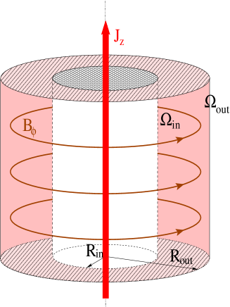
Figure 1: The conducting fluid resides between two concentric cylinders with radii $R_{\mathrm{in}}$ and $R_{\mathrm{out}}$ rotating with ${\it\Omega}_{\rm in}$ and ${\it\Omega}_{\rm out}$. $B_{\phi}$ is the magnetic field due to axial currents inside and outside the inner cylinder.

The fluid confined between the cylinders is assumed to be incompressible with uniform density and dissipative with the kinematic viscosity $\nu$ and the magnetic diffusivity $\eta$.

Derived from the conservation law of angular momentum the rotation law ${\it\Omega}(R)$ in the fluid is

$${\it\Omega}(R)=a+\frac{b}{R^{2}}$$ (2)

with

$$a=\frac{\mu_{\it\Omega}-\hat{\eta}^{2}}{1-\hat{\eta}^{2}}{\it\Omega}_{\rm in},\qquad b=\frac{1-\mu_{\it\Omega}}{1-\hat{\eta}^{2}}R_{\mathrm{in}}^{2}{\it\Omega}_{\rm in},$$ (3)

where

$$\hat{\eta}=\frac{R_{\rm{in}}}{R_{\rm{out}}},\qquad\qquad\qquad\mu_{\it\Omega}=\frac{{\it\Omega}_{\rm{out}}}{{\it\Omega}_{\rm{in}}}.$$ (4)

${\it\Omega}_{\rm in}$ and ${\it\Omega}_{\rm out}$ are the imposed rotation rates of the inner and outer cylinders with radii $R_{\rm in}$ and $R_{\rm out}$. After the Rayleigh stability criterion the flow is hydrodynamically stable for $\mu_{\it\Omega}>\hat{\eta}^{2}$. We are only interested in hydrodynamically stable regimes so that $\mu_{\it\Omega}>\hat{\eta}^{2}$ must be fulfilled. Rotation laws with ${\rm d}{\it\Omega}/{\rm d}R>0$ are described by $\mu_{\it\Omega}>1$ and rotation laws with ${\rm d}{\it\Omega}/{\rm d}R<0$ by $\mu_{\it\Omega}<1$. $\mu_{\it\Omega}=1$ gives the case of rigid rotation.

Also the magnetic profiles are restricted for real fluids. The solution of the stationary induction equation without inducing shear reads

$$B_{\phi}=AR+\frac{B}{R}.$$ (5)

in cylinder geometry. $A$ and $B$ are the fundamental quantities; the term $AR$ in Eq. (5) corresponds to uniform axial currents with $I=2A$ everywhere within $R<R_{\rm out}$, and $B/R$ corresponds to a uniform additional current only within $R<R_{\rm in}$. In the present paper we generally put $B=0$ with the consequence that the azimuthal magnetorotational instability (AMRI) does not appear. The behavior of the toroidal field is thus only due to TI for magnetic fields which are increasing outwards.

It is useful to define the quantity

$$\mu_{B}=\frac{B_{\rm{out}}}{B_{\rm{in}}}=\frac{AR_{\rm out}+B/R_{\rm out}}{AR_{\rm in}+B/R_{\rm in}},$$ (6)

measuring the variation of $B_{\phi}$ across the gap. Vanishing $B$ leads to $\mu_{B}=1/\hat{\eta}$. For $\hat{\eta}\to 1$ this choice is so close to the current-free solution $\mu_{B}=\hat{\eta}$ that the field becomes unstable against perturbations with $m=1$ only for very high Hartmann numbers.

In the following we fix $\mu_{B}=1/\hat{\eta}$ but we shall vary the magnetic Prandtl number

$$\rm Pm=\frac{\nu}{\eta},$$ (7)

and also the values of $\mu_{\it\Omega}$. If the results are to be applied to parts of the solar convection zone the magnetic Prandtl number must be replaced by its value of order unity for the turbulent medium.

3 Equations and numerical model

The dimensionless MHD equations for incompressible fluids are

$${\rm Re}\frac{\partial\mbox{\boldmath$u$}}{\partial t}+{\rm Re}(\mbox{\boldmath$u$}\cdot\nabla)\mbox{\boldmath$u$}=-\nabla P+\Delta\mbox{\boldmath$u$}+{\mathrm{Ha}^{2}}\mathop{\rm rot}\nolimits\mbox{\boldmath$B$}\times\mbox{\boldmath$B$},$$

$${\rm Rm}\frac{\partial\mbox{\boldmath$B$}}{\partial t}=\Delta\mbox{\boldmath$B$}+{\rm Rm}\mathop{\rm rot}\nolimits(\mbox{\boldmath$u$}\times\mbox{\boldmath$B$}),$$ (8)

with $\mathop{\rm div}\nolimits{\mbox{\boldmath$u$}}=\mathop{\rm div}\nolimits{\mbox{\boldmath$B$}}=0$ and with the Hartmann number

$$\mathrm{Ha}=\frac{B_{\rm in}D}{\sqrt{\mu_{0}\rho\nu\eta}}.$$ (9)

Here $D=\sqrt{R_{\mathrm{in}}(R_{\mathrm{out}}-R_{\mathrm{in}})}$ is used as the unit of length, $\eta/D$ as the unit of velocity and $B_{\rm in}$ as the unit of magnetic fields. Frequencies including the rotation ${\it\Omega}$ are normalized with the inner rotation rate ${\it\Omega}_{\rm in}$. The Reynolds number $\mathrm{Re}$ is defined as

$$\mathrm{Re}=\frac{{\it\Omega}_{\rm in}D^{2}}{\nu}$$ (10)

and the magnetic Reynolds number as

$$\rm Rm=\frac{{\it\Omega}_{\rm in}D^{2}}{\eta}.$$ (11)

It appears here as useful to work with the ‘mixed’ Reynolds number

$$\rm Rem=\sqrt{\rm Re\cdot Rm}$$ (12)

which is symmetric in $\nu$ and $\eta$ as it is also the Hartmann number. For ${\rm Pm}=1$ it is ${\rm Re}={\rm Rm}={\rm Rem}$. It is sometimes useful to use the Lundquist number ${\rm S}=\sqrt{\rm Pm}\ {\rm Ha}$. The ratio of Rem and Ha,

$${\rm Mm}=\frac{{\rm Rem}}{{\rm Ha}},$$ (13)

is called the magnetic Mach number.

Applying the usual normal mode analysis, we look for solutions of the linearized equations of the form

$$F=F(R){\rm{exp}}\bigl{(}{\rm{i}}(kz+m\phi+\omega t)\bigr{)}.$$ (14)

Using Eq. (14), linearizing the Eq. (8) and representing the result as a system of first order equations, one finds

$$\frac{{\rm d}u_{R}}{{\rm d}R}+\frac{u_{R}}{R}+{\textrm{i}}\frac{m}{R}u_{\phi}+{\textrm{i}}ku_{z}=0,$$

$$\frac{{\rm d}P}{{\rm d}R}+{\textrm{i}}\frac{m}{R}\phi_{u}+{\textrm{i}}kZ+\left(k^{2}+\frac{m^{2}}{R^{2}}\right)u_{R}+$$

$$\qquad\qquad\qquad+{\textrm{iRe}}(\omega+m{\it\Omega})u_{R}-2{\it\Omega}{\textrm{Re}}u_{\phi}-$$

$$\qquad\qquad\qquad-{\textrm{iHa}}^{2}mAb_{R}+2{\textrm{Ha}}^{2}Ab_{\phi}=0,$$

$$\frac{{\rm d}\phi_{u}}{{\rm d}R}-\left(k^{2}+\frac{m^{2}}{R^{2}}\right)u_{\phi}-{\textrm{iRe}}(\omega+m{\it\Omega})u_{\phi}+$$

$$\qquad\qquad\qquad+2{\textrm{i}}\frac{m}{R^{2}}u_{R}-\frac{{\textrm{Re}}}{R}\frac{{\rm d}}{{\rm d}R}\left(R^{2}{\it\Omega}\right)u_{R}+$$

$$\qquad\qquad\qquad+2{\textrm{Ha}}^{2}Ab_{R}+{\textrm{iHa}}^{2}mAb_{\phi}-{\textrm{i}}\frac{m}{R}P=0,$$

$$\frac{{\rm d}Z}{{\rm d}R}+\frac{Z}{R}-\left(k^{2}+\frac{m^{2}}{R^{2}}\right)u_{z}-{\textrm{iRe}}(\omega+m{\it\Omega})u_{z}-$$

$$\qquad\qquad\qquad-{\textrm{i}}kP+{\textrm{iHa}}^{2}mAb_{z}=0,$$

$$\frac{{\rm d}b_{R}}{{\rm d}R}+\frac{b_{R}}{R}+{\textrm{i}}\frac{m}{R}b_{\phi}+{\textrm{i}}kb_{z}=0,$$

$$\frac{{\rm d}b_{z}}{{\rm d}R}-\frac{{\textrm{i}}}{k}\left(k^{2}+\frac{m^{2}}{R^{2}}\right)b_{R}+{\textrm{PmRe}}\frac{1}{k}(\omega+m{\it\Omega})b_{R}+$$

$$\qquad\qquad\qquad+\frac{1}{k}\frac{m}{R}\phi_{B}-\frac{1}{k}mAu_{R}=0,$$

$$\frac{{\rm d}\phi_{B}}{{\rm d}R}-\left(k^{2}+\frac{m^{2}}{R^{2}}\right)b_{\phi}-{\textrm{iPmRe}}(\omega+m{\it\Omega})b_{\phi}+$$ (15)

$$+{\textrm{i}}\frac{2m}{R^{2}}b_{R}-Ru_{R}+{\textrm{PmRe}}R\frac{{\rm d}{\it\Omega}}{{\rm d}R}b_{R}+{\textrm{i}}mAu_{\phi}=0,$$

where $\phi_{u}$, $Z$ and $\phi_{B}$ are defined as

$$\phi_{u}=\frac{{\rm d}u_{\phi}}{{\rm d}R}+\frac{u_{\phi}}{R},\ \ \ \ Z=\frac{{\rm d}u_{z}}{{\rm d}R},\ \ \ \ \phi_{B}=\frac{{\rm d}b_{\phi}}{{\rm d}R}+\frac{b_{\phi}}{R}$$ (16)

and $A=1/R_{\rm in}$ ($R_{\rm in}$ in units of $D$).

An appropriate set of ten boundary conditions is needed to solve the system (15). For the velocity the boundary conditions are always no-slip,

$$u_{R}=u_{\phi}=u_{z}=0.$$ (17)

For conducting walls the radial component of the field and the tangential components of the current must vanish, yielding

$${\rm d}b_{\phi}/{\rm d}R+b_{\phi}/R=b_{R}=0.$$ (18)

These boundary conditions are applied at both $R_{\rm{in}}$ and $R_{\rm{out}}$. The wave number is varied as long as for given Hartmann number the Reynolds number takes its minimum. The procedure is already described in detail by Shalybkov, Rüdiger & Schultz (2002). One immediately finds that the sign of the real wave number $k$ is free so that with the solution for $k$ also another one with $-k$ exists. For containers bounded in $z$ standing waves can thus develop.

For insulating walls the boundary conditions are more complicated (see Rüdiger et al. 2007b).

The necessary and sufficient condition for the stability of toroidal fields in ideal Taylor-Couette flows against axisymmetric perturbations is by Michael (1954) and reads

$$\frac{1}{R^{3}}\frac{{\rm{d}}}{{\rm{d}}R}(R^{2}\Omega)^{2}-\frac{R}{\mu_{0}\rho}\frac{{\rm{d}}}{{\rm{d}}R}\left(\frac{B_{\phi}}{R}\right)^{2}>0.$$ (19)

Fields which are not steeper than $B_{\phi}\propto R$ are thus always stable against $m=0$ perturbations if the rotation law is also stable. Tayler (1973) found the necessary and sufficient condition

$$\frac{{\rm d}}{{\rm d}R}\left(RB_{\phi}^{2}\right)<0$$ (20)

for stability of an ideal nonrotating fluid against nonaxisymmetric disturbances. Our field profile $B_{\phi}=AR$ is thus stable against $m=0$ and unstable for sufficiently large field amplitudes, i.e. ${\rm Ha}>{\rm Ha}_{\rm crit}$. The same is true for nearly uniform fields with $\mu_{B}\simeq 1$. A general criterion for rotating flows does not exist.

First the system (15) is used to demonstrate that for resting cylinders the ${\rm Ha}_{\rm crit}$ does not depend on the magnetic Prandtl number Pm. To this end in the equations all terms resulting from the rotational influence are canceled. The frequency $\omega$ is replaced by $\omega/{\rm Re}$. Furthermore, the flow components $u_{\phi}$ and $u_{z}$ are replaced by $-{\rm i}u_{\phi}$ and $-{\rm i}u_{z}$ and the field component $b_{R}$ is replaced by ${\rm i}b_{R}$. It results

$$\frac{{\rm d}u_{R}}{{\rm d}R}+\frac{u_{R}}{R}+\frac{m}{R}u_{\phi}+ku_{z}=0,$$

$$\frac{{\rm d}P}{{\rm d}R}+\frac{m}{R}\phi_{u}+kZ+\left(k^{2}+\frac{m^{2}}{R^{2}}\right)u_{R}+$$

$$\qquad\qquad\qquad+{\textrm{i}}\omega u_{R}+\frac{{\textrm{Ha}}^{2}m}{R_{\rm in}}b_{R}+\frac{2{\textrm{Ha}}^{2}}{R_{\rm in}}b_{\phi}=0,$$

$$\frac{{\rm d}\phi_{u}}{{\rm d}R}-\left(k^{2}+\frac{m^{2}}{R^{2}}\right)u_{\phi}-{\textrm{i}}\omega u_{\phi}-2\frac{m}{R^{2}}u_{R}-$$

$$\qquad\qquad\qquad-\frac{2{\textrm{Ha}}^{2}}{R_{\rm in}}b_{R}-\frac{{\textrm{Ha}}^{2}m}{R_{\rm in}}b_{\phi}+\frac{m}{R}P=0,$$

$$\frac{{\rm d}Z}{{\rm d}R}+\frac{Z}{R}-\left(k^{2}+\frac{m^{2}}{R^{2}}\right)u_{z}-{\textrm{i}}\omega u_{z}+$$

$$\qquad\qquad\qquad+kP-\frac{{\textrm{Ha}}^{2}m}{R_{\rm in}}b_{z}=0,$$

$$\frac{{\rm d}b_{R}}{{\rm d}R}+\frac{b_{R}}{R}+\frac{m}{R}b_{\phi}+kb_{z}=0,$$

$$\frac{{\rm d}b_{z}}{{\rm d}R}+\frac{1}{k}\left(k^{2}+\frac{m^{2}}{R^{2}}\right)b_{R}+{\textrm{Pm}}\frac{{\rm i}}{k}\omega b_{R}+$$

$$\qquad\qquad\qquad+\frac{m}{kR}\phi_{B}-\frac{m}{kR_{\rm in}}u_{R}=0,$$

$$\frac{{\rm d}\phi_{B}}{{\rm d}R}-\left(k^{2}+\frac{m^{2}}{R^{2}}\right)b_{\phi}-{\textrm{iPm}}\omega b_{\phi}-$$ (21)

$$\qquad\qquad\qquad-\frac{2m}{R^{2}}b_{R}-Ru_{R}+\frac{m}{R_{\rm in}}u_{\phi}=0,$$

Note that the magnetic Prandtl number only survives together with ${\rm i}\omega$ which is purely imaginary for marginal instability. Hence, in the real part of the system (21) the frequency terms including the Pm do not appear. The only free parameter in the real part of the system (21), therefore, is the critical Hartmann number which results thus as equal for all Pm. Shalybkov (2006) has given a similar result but only for $m=0$.

Figure 2: The critical Hartmann number for ${\it\Omega}=0$ for various container gaps ($\hat{\eta}$) between conducting cylinders. The numbers are valid for all magnetic Prandtl numbers, see text.

The Hartmann numbers ${\rm Ha}_{\rm crit}$ for various $\hat{\eta}$ are given in Fig. 2. They vary over many orders of magnitude and become very small for wide gaps ($\hat{\eta}\to 0$). For small $\hat{\eta}$ the critical Hartmann number vanishes like

$${\rm Ha}_{\rm crit}\propto{\hat{\eta}}^{1.5}$$ (22)

with a factor of about 25. Our calculation with the smallest $R_{\rm in}$ concern $\hat{\eta}=0.001$ and lead to $\rm Ha=0.00075$.

In the present paper the gap between the cylinders is assumed as narrow ($\hat{\eta}=0.95$) and in another computation as wide ($\hat{\eta}=0.05$) so that the unit of distances, $D$, is the same in both cases for fixed outer radius. The narrow gap model serves to astrophysical discussions (solar tachocline, neutron star crust, supergranulation layer) while the wide gap results are needed to prepare future laboratory experiments. We have shown with similar models that indeed wide gaps are much more suitable for TI experiments with liquid metals like sodium or gallium than narrow gaps (Rüdiger et al. 2007b).

4 Narrow gap

For $\hat{\eta}=0.95$ it is $\mu_{B}=1.05$. The critical Hartmann number for $\rm Re=0$ is 3061 for all Pm (see Fig. 2). The Rayleigh limit for centrifugal instability is $\mu_{\it\Omega}=\hat{\eta}^{2}=0.9025$.

4.1 Rigid rotation

We start with the simplest case of the interaction of toroidal field and global rotation, i.e. with the marginal instability for rigid rotation ($\mu_{\it\Omega}=1$).

Figure 3: Narrow gap ($\hat{\eta}=0.95$): The suppression of the TI by rigid rotation. The curves are marked with their magnetic Prandtl number Pm. The rotational suppression of TI is weaker for $\rm Pm\neq 1$ than for $\rm Pm=1$. Rotating fluids with $\rm Pm=1$ allow the strongest fields to be stable.

The results of the calculations are shown in Fig. 3 in the plane Rem-Ha. As we already know the critical Hartmann number Ha for $\rm Rem=0$ does not depend on the magnetic Prandtl number. The new result is that the critical Ha always grows for growing rotation rate. This is the stabilizing action of rotation. In the representation of Fig. 3 (where the parameters on both axes are symmetric in $\nu$ and $\eta$) the growth of the critical magnetic amplitudes is strongest for ${\rm Pm}=1$ but it becomes weaker for ${\rm Pm}\neq 1$. For ${\rm Rem}\lower 1.72218pt\hbox{$\;\buildrel<\over{\scriptstyle\sim}\;$}500$ the differences of the critical magnetic fields for Pm varying over three orders of magnitude are surprisingly small.

For higher values of Rem the curves seem to represent a linear relation between Rem and Ha. Note that in Fig. 3 the magnetic Mach number

$${\rm Mm}=\frac{{\it\Omega}D}{B_{\rm in}/\sqrt{\mu_{0}\rho}}$$ (23)

is the smallest for ${\rm Pm}=1$. If this behavior remained true also for much higher Ha then the consequences should be strong: In turbulent fluids and/or in simulations with ${\rm Pm}=1$ rather strong magnetic fields remain stable which for the real $\mathrm{Pm}\neq 1$ are already unstable. For small Pm (stellar radiative interior) and high Pm (galaxies, neutron stars) the magnetic instability is much more efficient and already works for much smaller magnetic field strengths.

For neutron stars the ratio (23) yields

$${\rm Mm}\simeq\frac{3\cdot 10^{14}\ {\rm Gauss}}{B_{\phi}},$$ (24)

so that $B_{\phi}\simeq 3\cdot 10^{14}$ Gauss is the critical value for the toroidal field. We have here used the numerical values ${\it\Omega}=100$ s^-1, $\rho\simeq 10^{13}$ g/cm³ and $H\simeq 3\cdot 10^{5}$ cm.

The same data are plotted in Fig. 4 in the Rm-S plane. Again the curves are marked with their magnetic Prandtl numbers. One can read this plot in the sense that rotation, magnetic field and magnetic diffusivity $\eta$ are given and the viscosity (in units of $\eta$) is varied. For high viscosity the fields must be much stronger to become unstable. One finds a distinct stabilizing influence of the viscosity. The rotational influence, however, is weaker for high viscosity.

The results are applied to the bottom of the convection zone. The theory of the advection-dominated dynamo requires the small value of $10^{11}$ cm²/s for the eddy diffusivity $\eta$ while the eddy viscosity $\nu$ should be larger for the explanation of the differential rotation pattern so that ${\rm Pm}\geq 10$. With ${\it\Omega}\simeq 2\cdot 10^{-6}$ s^-1 and $D\simeq 10^{10}$ cm we find ${\rm Rm}\simeq 2000$. Figure 4 yields $\rm S\leq 10^{4}$ for stability. With $\rho\simeq 0.1$ g/cm³ the upper limit for stable toroidal fields becomes 100 kGauss. Stronger fields will not be stable against the Tayler instability. This value does not grow if the non-uniformity of the rotation (i.e. superrotation) is included due to the high value of Pm (see below).

Figure 4: The same as in Fig. 3 but for fixed magnetic diffusivity $\eta$ and varied viscosity. High viscosity stabilizes the magnetic fields and reduces the rotational influence.

4.2 Nonuniform rotation

The form of the rotation law is now changed for various magnetic Prandtl numbers. Rotation laws with negative shear (here $\mu_{\it\Omega}=0.5$ and $\mu_{\it\Omega}=0.92$) and superrotation laws (here $\mu_{\it\Omega}=1.07$) are investigated. The rotation law with $\mu_{\it\Omega}=0.5$ is centrifugally unstable also without magnetic field. It is given only for demonstration. The remaining rotation laws are stable in the hydrodynamic regime. One finds the numerical results for marginal stability of the $m=1$ mode in Fig. 5. Superrotation stabilizes the field more than solid-body rotation. For subrotation the behavior is opposite. While for rigid rotation and superrotation the critical Hartmann numbers grow for growing Reynolds number Rem, for subrotation the Ha become smaller so that finally the shear becomes superAlfvénic. This effect is in accordance with the Acheson relation (1).

Figure 5: Reynolds number vs. Hartmann number of the TI for subrotation ($\mu_{\it\Omega}=0.5$, $\mu_{\it\Omega}=0.92$), rigid rotation ($\mu_{\it\Omega}=1$) and superrotation ($\mu_{\it\Omega}=1.07$). Note the rotational quenching for $\mu_{\it\Omega}=1$, the strong destabilization by subrotation and the stabilization by superrotation. Conducting cylinder walls, $\hat{\eta}=0.95$, $\rm Pm=1$.

Figure 6: The same as in Fig. 5 for $\mu_{\it\Omega}=0.92$ but for much higher Reynolds numbers. The rotational destabilization does only hold for medium Reynolds numbers. For faster rotation the rotational stabilization dominates. $\rm Pm=1$.

This finding, however, cannot be the final answer. Very intensive differential rotation always tends to suppress nonaxisymmetric magnetic patterns. We therefore expect that for higher Reynolds numbers the Eq. (1) looses its meaning. In Fig. 6 the marginal-instability curve for $\mu_{\it\Omega}=0.92$ is thus followed to very high values of the Reynolds number. The result of the calculations is that also for subrotation the basic rotation finally suppresses the instability if $\rm Rem\lower 1.72218pt\hbox{$\;\buildrel>\over{\scriptstyle\sim}\;$}3000$.

Up to this value the differential rotation acts destabilizing. In regions of convection zones with ${\rm d}{\it\Omega}/{\rm d}R<0$ much weaker toroidal fields become unstable than for ${\rm d}{\it\Omega}/{\rm d}R>0$. This finding should have strong implications for the electrodynamics of rotating stars. Young stars typically rotate ten times faster then old stars such as the Sun. For the supergranulation part of the solar convection zone the magnetic Reynolds number does not exceed (say) 300. For younger solar-type stars, however, it can easily reach the value of 3000. For all Pm and a Reynolds number of order 3000 the field becomes unstable already for very small Ha of order 100. Hence, the maximum stable toroidal fields in this zone for which the helioseismology provides a clear subrotation is much weaker for fast rotating stars than for the slow-rotating Sun. Fast rotators are thus not able to accumulate strong toroidal field which could be observed as starspots close to the equator.

In Fig. 5 also the (dashed) curve for ${\mu}_{\it\Omega}=0.5$ is given for comparison. Such a rotation law is unstable without magnetic field for $m\geq 0$. The magnetic field additionally destabilizes the rotation law so that for $\rm Ha=3061$ the TI works even without any rotation.

The differences of the results for subrotation and for superrotation only appear for faster rotation but it is until now unclear how strong the magnetic fields must be. The calculations for nonuniform rotation laws must be extended to smaller and higher magnetic Prandtl numbers. Figure 7 gives the results for $\rm Pm=0.1$ and $\rm Pm=10$. They can be best written with the characteristic numbers Rem and Ha because in this formulation the differences for the small and the large magnetic Prandtl number are smallest. For small magnetic Prandtl number the stabilizing influence of superrotation is stronger than for high magnetic Prandtl numbers. Note that for $\rm Pm=10$ the stabilization of the magnetic field by superrotation is even smaller than that of rigid rotation. It is not clear whether for even larger magnetic Prandtl numbers rotation laws with positive shear become able to destabilize the magnetic fields.

Written with Rem and Ha one finds for given rotation law with $\mu_{\it\Omega}\simeq 1$ that $\rm Pm=1$ yields the most effective stabilization of the toroidal magnetic field. For $\rm Pm\neq 1$ the stabilization is stronger for small Pm than for large Pm. The differences, however, are small. For subrotation ($\mu_{\it\Omega}<1$) the very effective rotational destabilization of the magnetic field hardly depends on the magnetic Prandtl number.

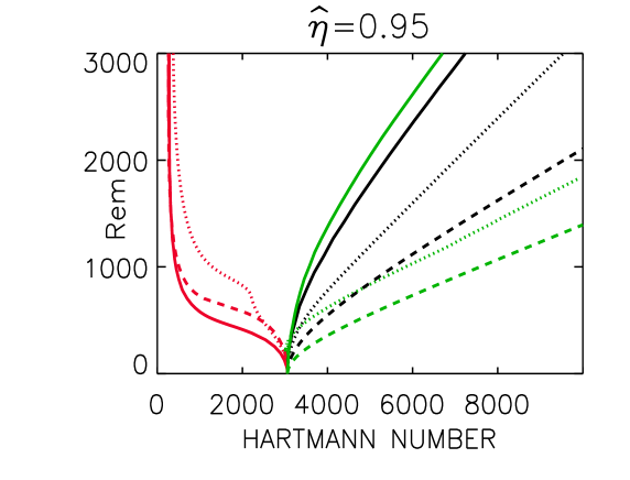
Figure 7: The same as in Fig. 5 but for $\rm Pm=0.1$ (dotted), $\rm Pm=1$ (dashed) and $\rm Pm=10$ (solid). The curves for negative shear ($\mu_{\it\Omega}=0.92$, subrotation) are red and the curves for positive shear ($\mu_{\it\Omega}=1.07$, superrotation) are green. For large Pm superrotation yields less stability than rigid rotation.

In summary, we have shown for the container with the narrow gap that without rotation the critical Hartmann number is $\rm Ha=3061$ independent of the magnetic Prandtl number. This value is increased for solid-body rotation and for superrotation but it is drastically reduced to about 100 for subrotation with ${\rm Rem}\geq 1000$. There is no strong dependence of these characteristic numbers on the magnetic Prandtl number. However, for too fast rotation (${\rm Rem}>3500$) the destabilization changes to rotational stabilization (see Fig. 6). On the other hand, the role of superrotation to stabilize the magnetic field changes to destabilization for too high magnetic Prandtl number.

4.3 The angular momentum transport

The solutions of the linear equations are free of an arbitrary real parameter of any sign. We do not know, therefore, the sign of the flow and/or the field. However, for quadratic expressions such as the correlation tensor or the electromotive force one can find the signs as all the solutions are multiplied with one and the same parameter.

Let us apply this idea to the angular momentum transport

$$T_{R}=\langle u_{R}^{\prime}u_{\phi}^{\prime}-\frac{1}{\mu_{0}\,\rho}B_{R}^{\prime}B_{\phi}^{\prime}\rangle.$$ (25)

The average procedure consists of an integration over the azimuth $\phi$. The question we shall answer is whether $T_{R}$ and ${\rm d}{\it\Omega}/{\rm d}R$ are anticorrelated. If this is true then the angular momentum flows towards the minimum of the angular velocity, and one can introduce an eddy viscosity $\nu_{\rm T}$ in accordance to

$$T_{R}=-\nu_{\rm T}R\frac{{\rm d}{\it\Omega}}{{\rm d}R}$$ (26)

with positive $\nu_{\rm T}$.

After normalization the expression (25) reads

$$T_{R}\simeq\langle u_{R}^{\prime}u_{\phi}^{\prime}\rangle-{\rm Ha}^{2}{\rm Pm}\langle B_{R}^{\prime}B_{\phi}^{\prime}\rangle.$$ (27)

In Fig. 8 the angular momentum (25) normalized with $\sqrt{\langle u_{R}^{\prime 2}u_{\phi}^{\prime 2}\rangle}$ is given. Without magnetic fields its absolute value must be smaller than unity. The Maxwell stress, however, may produce higher values. We take from Fig. 8 that in the linear theory the magnetic contribution is surprisingly small.

Figure 8: The angular momentum transport (25) for subrotation ($\mu_{\it\Omega}=0.92$, top) and superrotation ($\mu_{\it\Omega}=1.07$, bottom). $\rm Re=500$, $\rm Pm=1$. The torque is positive for subrotation and negative for superrotation. The values are normalized with the turbulence intensity $U=\sqrt{\langle u_{R}^{\prime 2}\rangle\langle u_{\phi}^{\prime 2}\rangle}$. Due to the Maxwell stress they can exceed unity.

For simplicity we only work here with ${\rm Pm}=1$. The angular momentum transport vanishes for rigid rotation and it is indeed anticorrelated with $\nabla{\it\Omega}$. The diffusion approximation (26) is thus possible. Its magnetic part is (only) of the same order than its kinetic part.

5 Wide gap

For $\hat{\eta}=0.05$ it is $\mu_{B}=1/\hat{\eta}=20$. The critical Hartmann number for $\rm Re=0$ is 0.31 for all Pm (see Fig. 9). The Rayleigh limit for centrifugal instability is $\mu_{\it\Omega}=\hat{\eta}^{2}=0.0025$.

5.1 Electric currents

The technical possibilities are now discussed to realize this Hartmann number in the laboratory working with liquid metals. Let $I_{\rm axis}$ be the axial current inside the inner cylinder and $I_{\rm fluid}$ the axial current between the inner and the outer cylinder. The assumption $B=0$ in Eq. (5) provides

$$\frac{I_{\rm fluid}}{R_{\rm out}^{2}-R_{\rm in}^{2}}=\frac{I_{\rm axis}}{R_{\rm in}^{2}}$$ (28)

as the current density is homogeneous. Hence,

$$\frac{I_{\rm fluid}}{I_{\rm axis}}=\frac{1-\hat{\eta}^{2}}{\hat{\eta}^{2}}=399$$ (29)

for $\hat{\eta}=0.05$. It is also clear that

$$B_{\rm in}=\frac{I_{\rm axis}}{5R_{\rm in}},$$ (30)

where $R$, $B$ and $I$ are measured in cm, Gauss and Amp.

Figure 9: The same as in Fig. 2 but for $\hat{\eta}\to 0$. The dotted line represents the algebraic expression $25\cdot{\hat{\eta}}^{1.5}$.

It follows

$$I_{\rm axis}=\frac{5R_{\rm in}{\rm Ha}}{D}\sqrt{\mu_{0}\rho\nu\eta}=5\sqrt{\frac{\hat{\eta}}{1-\hat{\eta}}}{\rm Ha}\sqrt{\mu_{0}\rho\nu\eta}.$$ (31)

With the limit (22) of Ha for small $\hat{\eta}$ one finds

$$I_{\rm fluid}=140\sqrt{1-\hat{\eta}}(1+\hat{\eta})\sqrt{\mu_{0}\rho\nu\eta}\ \ [{\rm Amp}].$$ (32)

With the numerical values for $\hat{\eta}=0.05$ and $\sqrt{\mu_{0}\rho\nu\eta}=25.6$ for the gallium-tin alloy used in the experiment PROMISE we find

$$I_{\rm fluid}=11.8\ {\rm Ha}\ \ [{\rm kAmp}]$$ (33)

for the electric current through the gallium and

$$I_{\rm axis}=29.5\ {\rm Ha}\ \ [{\rm Amp}]$$ (34)

for the current along the axis. With ${\rm Ha}=0.31$ for $\hat{\eta}=0.05$ (see Fig. 9) the results are $I_{\rm fluid}=3.66$ kAmp and $I_{\rm axis}=9.1$ Amp.

In the limit $\hat{\eta}\to 0$ the total current through the fluid conductor becomes 3.20 kAmp which is within the present-day technical possibilities. It should thus be possible to realize the nonaxisymmetric current-driven TI in the MHD laboratory also with fluids of small magnetic Prandtl number, e.g. with sodium and gallium.

5.2 Uniform rotation

Figure 10 gives for the wide-gap container the rotational quenching of the TI for various values of the magnetic Prandtl number Pm similar to Fig. 3 for the narrow gap. Again the lines for marginal instability in the Rem-Ha plane are straight lines. The line for $\rm Pm=1$ gives the ultimate stabilization by rigid rotation. A stronger stabilization does not exist. Hence, if ${\rm Rem}\lower 1.72218pt\hbox{$\;\buildrel<\over{\scriptstyle\sim}\;$}6\cdot{\rm Ha}$ then the fluid is always unstable (for rigid rotation). The rotational stabilization is much weaker for all $\rm Pm\neq 1$. It is in particular weak for very small Pm.

Figure 10: The same as in Fig. 3 but for $\hat{\eta}=0.05$. The curves are marked with the magnetic Prandtl numbers. Again rotating fluids with $\rm Pm=1$ undergo the strongest stabilization.

The question is whether also the rotational stabilization of the TI can be probed in the laboratory. Therefore, the rigidly rotating wide-gap container is considered also for the very small magnetic Prandtl numbers of fluid metals. The magnetic Prandtl number of sodium is about $\rm Pm=10^{-5}$, and for gallium it is about $\rm Pm=10^{-6}$. Without rotation the critical Hartmann number is 0.31 for this container (independent of Pm). With rotation the numerical results are given in Fig. 11. We find the rotational stabilization also existing for fluids with their small Pm. For not too fast rotation the differences of the resulting critical Ha are very small for both the fluid conductors so that experiments with gallium are also possible. For a (small) Reynolds number of order 1000 the marginal-stable magnetic field is about two times higher than for $\rm Re=0$. It should thus not be too complicated to find the basic effect for the rotational suppression of TI – which proves to be important both for the rapid-rotating hot MS stars and also for neutron stars – in the MHD laboratory.

Figure 11: The suppression of the TI in a wide-gap container by rigid rotation for $\rm Pm=10^{-5}$ and $\rm Pm=10^{-6}$. The standard Reynolds number (10) is given for experimental applications. $\hat{\eta}=0.05$, $\mu_{B}=20$.

The curves in Fig. 11 do not become more steep for $\rm Pm\to 0$. There is no visible difference between the curves for ${\rm Pm}=10^{-6}$ and ${\rm Pm}=0$.

6 Conclusions

In this paper the interplay of Tayler instability and rotation for incompressible fluids of uniform density filling the gap between the cylinders of a Taylor-Couette container is considered. The toroidal field is the result of an electric current of homogeneous density. It is shown that for zero rotation the critical magnetic field amplitudes for marginal instability does not depend on the magnetic Prandtl number. The critical magnetic field strongly depends on the gap width. It is very high for small gaps and it this rather low for wide gaps. For small enough inner radius $R_{\rm in}$ the critical Hartmann number (of the inner field) runs as $R_{\rm in}^{1.5}$. The resulting electric currents necessary for TI with $m=1$ are 3.66 kAmp if the material is the same gallium-tin alloy as used in the experiment PROMISE. Such currents can easily be produced in the laboratory.

For a narrow gap with $\hat{\eta}=0.95$ the rotational quenching of the TI is studied in detail. Figure 3 displays the rotational stabilization for various magnetic Prandtl numbers. For the normalization of the basic rotation a ‘mixed’ Reynolds number (12) is used in which – as in the Hartmann number – the viscosities $\nu$ and $\mu$ are symmetric. The ratio of this Reynolds number Rem and the Hartmann number is basically free of any diffusivity. For fast enough rotation just this ratio describes the rotational quenching of TI for various Pm. In this representation the results for Pm between 0.01 and 10 are rather simple. The most effective stabilization of TI happens for $\rm Pm=1$. It is weaker for both smaller Pm and higher Pm. This is an unexpected result which may warn that many numerical simulations with $\rm Pm\simeq 1$ could overlook the nonaxisymmetric instability of strong toroidal fields.

Also the inclusion of differential rotation leads to surprising results. For $\rm Pm=1$ the Fig. 5 presents the basic differences for rotation laws with different signs of ${\rm d}{\it\Omega}/{\rm d}R$. While superrotation always stabilizes the magnetic field, there is a dramatic destabilization phenomenon by subrotation for medium rotation rates. This is the effect announced with Eq. (1) by Acheson (1978). For slow and fast rotators (old and young stars with outer convection zones) with negative shear the toroidal magnetic fields have a very different stability behavior. Slowly rotating (old) stars with small Rem can accumulate much stronger magnetic fields than young stars with their larger Rem. However, if the rotation is too strong then the nonaxisymmetric instabilities are more and more destroyed by the very strong shear (see Fig. 6).

Our calculations demonstrate that rigid rotation always stabilizes the magnetic field against the nonaxisymmetric TI. We have also shown that this rotational stabilization should be observable in the laboratory. Figure 11 provides the result that the critical Hartmann number in a wide-gap container of $\hat{\eta}=0.05$ can be increased by a factor of two by a rigid rotation of Reynolds number 1000. For the gallium-tin alloy with its molecular viscosity of $3.4\cdot 10^{-3}$ cm²/s this Reynolds number is reached for a rotation frequency of about $11.4/R_{\rm out}^{2}$ Hz with $R_{\rm out}$ in cm. The rotation frequency of 0.11 Hz for $R_{\rm out}\simeq 10$ cm is rather small. For the same container one needs the electric current of 7.32 kAmp through the gallium-tin alloy to realize the Tayler instability in the rotating fluid conductor.

References

- [1] Acheson, D.J.: 1978, RSPTA 289, 459
- [2] Balbus, S.A., Hawley, J.F.: 1992, ApJ 400, 610
- [3] Chandrasekhar, S.: 1961, Hydrodynamic and Hydromagnetic Stability, Clarendon Press, Oxford
- [4] Chanmugam, G.: 1979, MNRAS 187, 769
- [5] Dubrulle, B., Knobloch, E.: 1993, A&A 274, 667
- [6] Howard, L.N., Gupta, A.S.: 1962, JFM 14, 463
- [7] Knobloch, E.: 1992, MNRAS 255, 25p
- [8] Kumar, S., Coleman, C.S., Kley, W.: 1994, MNRAS 266, 379
- [9] Maeder, A., Meynet, G.: 2005, A&A 440, 1041
- [10] Michael, D.H.: 1954, Mat 1, 45
- [11] Ogilvie, G.I., Pringle, J.E.: 1996, MNRAS 279, 152
- [12] Pessah, M.E., Psaltis, D.: 2005, ApJ 628, 879
- [13] Pitts, E., Tayler, R.J.: 1985, MNRAS 216, 139
- [14] Rüdiger, G., Hollerbach, R., Schultz, M., Elstner, D.: 2007a, MNRAS 377, 1481
- [15] Rüdiger, G., Schultz, M., Shalybkov, D., Hollerbach, R.: 2007b, Phys Rev E 76, 056309
- [16] Shalybkov, D.: 2006, Phys Rev E 73, 016302
- [17] Shalybkov, D., Rüdiger, G., Schultz, M.: 2002, A&A 395, 339
- [18] Tagger, M., Pellat, R., Coroniti, F.V.: 1992, ApJ 393, 708
- [19] Tayler, R.J.: 1957, PPSB 70, 31
- [20] Tayler, R.J.: 1973, MNRAS 161, 365
- [21] Vandakurov, Yu.V.: 1972, SvA 16, 265
- [22]