Conductance of telescoped double-walled nanotubes from perturbation calculations

Abstract

In a telescoped double-walled nanotube (TDWNT), with the inner tube partially extracted from the outer tube, the total current is forced to flow between the layers. Considering the interlayer Hamiltonian as a perturbation, we can obtain an analytic formula for the interlayer conductance. The accuracy of the perturbation formula is systematically improved by including higher-order terms. The interlayer interaction effective in the perturbation formula is the product of the interlayer Hamiltonian and the wave function. It clarifies the effects of the spatial range of the interlayer Hamiltonian and the band energy shift.

I Introduction

Electronic and mechanical properties of single-walled nanotubes (SWNTs) originate from the $\pi$ and $\sigma$ bonds in their honeycomb lattice.tubeHamada ; NT-book ; review Although the interlayer bonds are considerably weaker than the intralayer $\pi$ and $\sigma$ bonds, they are important for the formation of double-walled nanotubes (DWNT), multi-walled nanotubes, and nanotube bundles. The telescoped double-walled nanotube (TDWNT) shown in Fig. 1 was formed from a DWNT by partially extracting the inner tube. Since the rigid honeycomb lattice is relatively unaffected by the weak interlayer bonds, the basic motions of the TDWNT are limited to the interlayer motions caused by relative slide and rotation between the outer and inner SWNTs. Attaching a piezoelectric electrode to each edge, where only a single monolayer exists, we can measure the relation between the interlayer motions and the $total$ current forced to flow between the layers. The interlayer motion and the interlayer force were investigated theoretically using molecular dynamics MD-phonon-sliding-shock-wave ; MD-telescope-friction ; LDA-interlayer-elastic ; MD-GHz-oscillator ; DWNT-interlayer-pot-R.Saito and experimentally by AFM and TEM.AFM-sidecontact-SWNTbridge ; AFM-SEM-nano-resonator ; AFM-telescope The interlayer conductances were also measured experimentally.exp-telescope-Zettl ; exp-telescope-Nakayama-conductance The relationship between the interlayer conductance and the interlayer motion can be used to construct nano electro-mechanical systems (NEMS), such as nano-mechanical switches, nano-switch and nano-displacement sensors.

The interlayer bond between atoms $\alpha$ and $\beta$ is represented by the interlayer Hamiltonian element $H_{\alpha,\beta}$. The interlayer motion influences the conductance through the change of these elements. Considering the interlayer Hamiltonian as a perturbation, we can show that the effective interlayer interaction is the product of the interlayer Hamiltonian and the wave function. Though this effective interlayer interaction ref1 was discussed in Ref.Tamura , its relation to the conductance was complicated. In the present paper, the perturbation formula simplifies this relation. The perturbation formula was not discussed in most of the preceding theoretical works about the conductances of TDWNTs Uryu-telescope ; telescope-Kim ; telescope-Buia ; telescope-comp-phys ; Kim ; telescope-Hasson ; telescope-Grace ; Tamura . In Refs. NT-FGR ; Turnney-Cooper , the perturbation formula was discussed but limited to the incommensurate interlayer configuration. The present paper shows that the perturbation formula is effective even for commensurate TDWNTs, e.g. the (5,5)-(10,10) TDWNT, despite their larger interlayer interaction. In order to confirm the validity of the perturbation theory, the effect of higher order terms , that was not discussed in Refs. NT-FGR ; Turnney-Cooper , is also examined.

Approximate analytical formulas in Refs. telescope-Grace ; telescope-Kim include fitting parameters other than the Hamiltonian. Though the fitting parameters are useful for precise reproduction of the exact results, they produce ambiguity about the relation between the conductance and the Hamiltonian. In the present paper, the perturbation formula is discussed for the interpretation of the relation between the Hamiltonian and the conductance. Thus the fitting parameters are excluded. Since there is no fitting parameter, agreement between the perturbation formula and the exact results is limited. Nevertheless the perturbation formula is effective in the interpretation when it reproduces qualitatively the relation between the Hamiltonian and the conductance.

The paper is organized as follows. The tight-binding (TB) model used in the present paper is described in Sec. II. The perturbation formulas are derived in Sec. III. The results of Ref.Tamura are reproduced by the perturbation formulas in Sec. IV A. Corrections of the TB Hamiltonian suggested by Refs. telescope-comp-phys ; Kim are analyzed in Sec. IV B and IV C. Summary and discussion are shown in Sec. V.

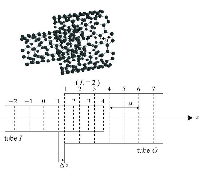
Figure 1: Telescoped double-walled nanotube (TDWNT).

II Tight-Binding Model

We considered the TDWNT composed of two armchair tubes, $(n_{O},n_{O})$ and $(n_{I},n_{I})$. The symbols $O$ and $I$ indicate the outer and inner tubes, respectively. As the interlayer distance must be close to that of graphite, only the case of $n_{O}=n_{I}+5$ was considered. Henceforth, the symbol $\mu$ indicates either $O$ or $I$. The cylindrical coordinates $(r,\theta,z)$ of the atoms in the tube $\mu$ are

$$(r,\theta,z)=\left(R_{\mu},\;\frac{\pi\chi_{l,j}}{6n_{\mu}}+\delta_{\mu,I}\Delta\theta,\;\frac{a}{2}j+\delta_{\mu,O}\Delta z\right)$$ (1)

with integers $l,j$, $\chi_{l,j}\equiv 6l-5-(-1)^{l+j}$, the lattice constant $a\equiv\sqrt{3}\times 0.142$ nm, and $R_{\mu}=\sqrt{3}an_{\mu}/(2\pi)$. Regarding the range of $j$, $j\geq 1$ for tube $O$ and $j\leq 2L$ for tube $I$, where $L$ is the number of unit cells in the overlap region. As shown in Fig. 1, the overlap length equals $(L-0.5)a-\Delta z$. Figure 2 shows the relationship between the integers $(l,j)$ and the coordinates $(\theta,z)$. The geometric structure and the definition of $(\Delta\theta,\Delta z)$ are the same as in Ref.Tamura , where $|\Delta\theta|<\pi/n_{O}$ and $|\Delta z|<a/4$.

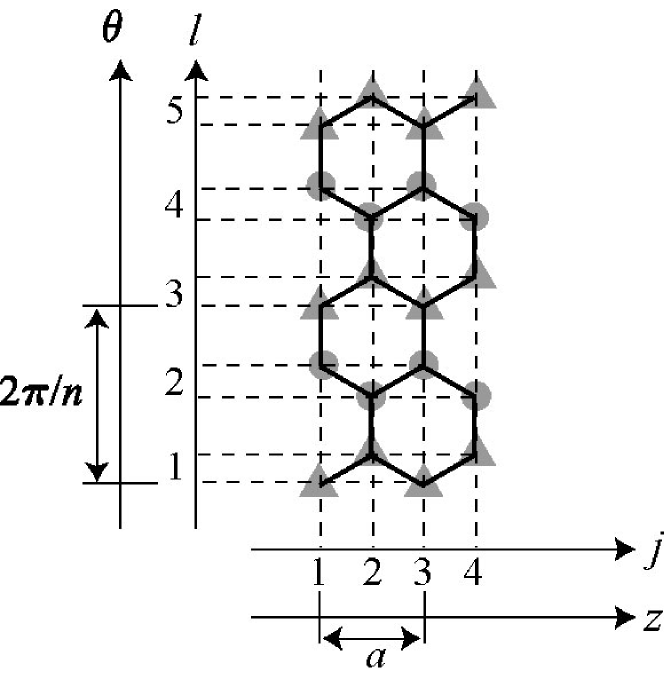
Figure 2: Relationship between integer indexes $(l,j)$ and coordinates $(\theta,z)$. Triangles and circles correspond to odd $l$ and even $l$, respectively.

The $\pi$ orbital at position (1) is denoted by $|\mu,l,j\,\rangle$ and is assumed to be orthonormal, i.e., $\langle\mu^{\;\prime},l^{\;\prime},j^{\;\prime}|\mu,l,j\,\rangle=\delta_{\mu,\mu^{\;\prime}}\delta_{l,l^{\;\prime}}\delta_{j,j^{\;\prime}}$, where ’bra’ and ’ket’ are used to simplify the notation. The Hamiltonian $H$ of the TDWNT is decomposed as $H=H^{(0)}_{I}+H^{(0)}_{O}+V$, where $H^{(0)}_{\mu}$ and $V$ correspond to the intralayer and interlayer Hamiltonian elements, respectively. The interlayer element between atom $\alpha=(O,l,j)$ and atom $\beta=(I,l^{\;\prime},j^{\;\prime})$ is represented by

$$\langle\alpha|V|\beta\rangle=\left\{\begin{array}[]{cc}(W+\Delta W)e^{\frac{d-r}{L_{c}}}\cos\theta_{\alpha,\beta}&\;\cdots r<r_{c}\\ 0&\;\cdots r>r_{c}\end{array}\right.$$ (2)

with $\theta_{\alpha,\beta}=\theta_{\alpha}-\theta_{\beta}$, inter-atomic distance $r$, constants $W=0.36$ eV, $d=0.334$ nm, $L_{c}=0.045$ nm, and cutoff radius $r_{c}$. The interlayer bonds were classified as ’AA’, ’BB’, or ’AB’ bonds. When either $\alpha$ or $\beta$ had an interlayer bond shorter than $r_{0}$ with the third atom $\gamma$ $(\neq\alpha,\beta)$ and $r>$ $r_{0}$, the bond between $\alpha$ and $\beta$ was classified as an AB bond. Tamura ; Lambin ; Charlier Here, $r_{0}=(a/\sqrt{3})\sqrt{(0.36)^{2}+(15/2\pi)^{2}}=0.34283$ nm,cut-off-note $\Delta W=-0.20$ eV for AB bonds, and $\Delta W=0$ for AA and BB bonds. The covalent bond character is the origin of the negative value of $\Delta W$, the small cutoff radius $r_{c}$, and the dependence on $\theta$. The intralayer elements were $-t=-2.75$ eV between nearest neighbors, $\varepsilon$ for the diagonal terms of $H^{(0)}_{O}$, and zero otherwise. Even when no interlayer interaction exists, the linear dispersion lines of tube $O$ shift from those of tube $I$ due to the difference in curvature causing $\sigma-\pi$ mixing. In the following discussions, this shift is called ’intrinsic’ and is distinct from the shift induced by interlayer interaction. Kim ; DWNT-band ; single-band-TB-2 The parameter $\varepsilon$ was introduced to represent this intrinsic shift.

The energy $E^{(\mu)}_{\sigma,k}$ and the wave function $|\mu,\sigma,k\}$ of an isolated SWNT were obtained from $H^{(0)}_{\mu}|\mu,\sigma,k\}=E^{(\mu)}_{\sigma,k}|\mu,\sigma,k\}$ as

$$E^{(\mu)}_{\sigma,k}=-2t\cos(ka/2)-t\sigma+\varepsilon\delta_{\mu,O}$$ (3)

$$|\mu,\sigma,k\}=\frac{1}{\sqrt{2}}\sum_{j}\exp(ikaj/2)|\mu,\sigma,j\,\rangle\rangle$$ (4)

and

$$|\mu,\sigma,j\,\rangle\rangle=\frac{1}{\sqrt{2n_{\mu}}}\sum_{l=1}^{2n_{\mu}}\sigma^{l}|\mu,l,j\,\rangle$$ (5)

with the wave number $k$ and the mirror symmetry $\sigma=\pm 1$. When $\varepsilon=0$ and $r_{c}=(a/\sqrt{3})\sqrt{(1.37)^{2}+(15/2\pi)^{2}}=$ 0.39085 nm,cut-off-note the total Hamiltonian $H=H^{(0)}_{I}+H^{(0)}_{O}+V$ becomes equivalent to that of Ref. Tamura . The reflection at the open edges $(j=1,2L)$ was neglected here, but will be considered in Sec. III B. The ket $|\mu,\sigma,j\,\rangle\rangle$ defined by Eq. (5) will be used in Sec. III B.

III Derivation of the perturbation formula

III.1 Fermi’s golden rule

Since the interlayer Hamiltonian element in Eq. (2) is much smaller than the intralayer $\pi$ bonding $t=2.75$ eV, it can be considered as a perturbation. According to Fermi’s golden rule (FGR), the probability of a transition caused by the perturbation $V$ per unit time is

$$P(O,\sigma,k|I,\sigma^{\;\prime},k^{\;\prime}) = \frac{4\pi^{2}}{h}\left|\left\{O,\sigma,k|V|I,\sigma^{\;\prime},k^{\;\prime}\right\}\right|^{2}$$ (6)

$$\times\delta(E^{(O)}_{\sigma,k}-E^{(I)}_{\sigma^{\;\prime},k^{\;\prime}}).$$

The density of states with positive group velocity was derived from Eq. (3) as

$$D^{(\mu)}_{\sigma}(E^{(\mu)}) = \frac{a}{2\pi}\left(\frac{d}{dk}E^{(\mu)}_{\sigma,k}\right)^{-1}$$ (7)

$$= \left(\pi\sqrt{4t^{2}-(E^{(\mu)}+\sigma t-\varepsilon\delta_{\mu,O})^{2}}\right)^{-1}$$

per unit cell of tube $\mu$. Note that the wave function (4) was also normalized per unit cell.

When the Fermi level $E_{F}$ is close to zero, the interlayer current $I$ can be estimated to be

$$I \simeq 2e\sum_{\sigma,\sigma^{\;\prime}}\int dE^{(O)}\int dE^{(I)}(f_{O}-f_{I})D^{(O)}_{\sigma}D^{(I)}_{\sigma^{\;\prime}}$$ (8)

$$\times P(O,\sigma,k|I,\sigma^{\;\prime},k^{\;\prime})$$

$$\simeq G_{0}V_{b}\sum_{\sigma,\sigma^{\;\prime}}F_{\sigma,\sigma^{\;\prime}}\left|\left\{O,\sigma,k^{(O)}_{\sigma}|V|I,\sigma^{\;\prime},k^{(I)}_{\sigma^{\;\prime}}\right\}\right|^{2},$$

where

$$F_{\sigma,\sigma^{\;\prime}}\equiv 4\pi^{2}d^{(O)}_{\sigma}d^{(I)}_{\sigma^{\;\prime}},$$ (9)

$G_{0}\equiv 2e^{2}/h$, $d^{(\mu)}_{\sigma}\equiv D^{(\mu)}_{\sigma}(E_{F})$, and $V_{b}$ denotes the bias voltage. The Fermi wave number $k^{(\mu)}_{\sigma}$ satisfies $E_{F}=-2t\cos(k^{(O)}_{\sigma}a/2)-t\sigma+\varepsilon$, $E_{F}=-2t\cos(k^{(I)}_{\sigma^{\;\prime}}a/2)-t\sigma^{\;\prime}$ and the positive group velocity, $\sin(k^{(\mu)}_{\sigma}a/2)>0$. As both the bias voltage $V_{b}$ and the temperature were close to zero, the Fermi-Dirac distribution function difference $f_{O}-f_{I}$ was replaced by $eV_{b}\delta(E_{F}-E^{(O)})$ in Eq. (8).

According to Landauer’s formula, on the other hand, the conductance $G=I/V_{b}$ is determined by

$$G=G_{0}\sum_{\sigma=\pm}\sum_{\sigma^{\;\prime}=\pm}T_{\sigma,\sigma^{\;\prime}},$$ (10)

where $T_{\sigma,\sigma^{\;\prime}}$ denotes the interlayer transmission rate from $|I,\sigma^{\;\prime},k^{\;\prime}\}$ to $|O,\sigma,k\}$. By comparing Eq. (8) to Eq. (10), an approximate formula for the transmission rate can be obtained as follows.

$$T_{\sigma,\sigma^{\;\prime}}=\frac{4}{3t^{2}}\left|\left\{O,\sigma,k^{(O)}_{\sigma}|V|I,\sigma^{\;\prime},k^{(I)}_{\sigma^{\;\prime}}\right\}\right|^{2}$$ (11)

Here we concentrate our discussion into cases where $|E_{F}|$ and $|\varepsilon|$ are much less than $t$, i.e.,

$$k^{(O)}_{\sigma}\simeq k^{(I)}_{\sigma}\simeq\frac{\pi}{a}\left(1+\sigma\frac{1}{3}\right),$$ (12)

$$\pi d^{(O)}_{\sigma}\simeq\pi d^{(I)}_{\sigma^{\;\prime}}\simeq\frac{1}{\sqrt{3}t},$$ (13)

and $F_{\sigma,\sigma^{\;\prime}}\simeq 4/(3t^{2})$.

Using Eqs. (4),(5) and (11),

$$T_{\sigma,\sigma^{\;\prime}}=\frac{1}{3t^{2}}\left|A^{(cor)}_{\sigma,\sigma^{\;\prime}}+A_{\sigma,\sigma^{\;\prime}}B_{\sigma,\sigma^{\;\prime}}\right|^{2}$$ (14)

where

$$A^{(cor)}_{\sigma,\sigma^{\;\prime}}\equiv\left(\frac{\bar{V}_{3,2}^{\sigma,\sigma^{\;\prime}}}{\omega_{\sigma}^{(O)}}-\bar{V}_{2,3}^{\sigma,\sigma^{\;\prime}}\omega_{\sigma^{\;\prime}}^{(I)}\right)\left(\frac{\omega_{\sigma^{\;\prime}}^{(I)}}{\omega_{\sigma}^{(O)}}\right)^{2L},$$ (15)

$$A_{\sigma,\sigma^{\;\prime}}\equiv\sum_{j=1}^{2}\sum_{s=-1}^{1}\bar{V}^{\sigma,\sigma^{\;\prime}}_{j,j+s}\left(\omega_{\sigma^{\;\prime}}^{(I)}\right)^{j+s}\left(\omega_{\sigma}^{(O)}\right)^{-j}$$ (16)

$$B_{\sigma,\sigma^{\;\prime}}\equiv\sum_{m=0}^{L-1}\left(\frac{\omega_{\sigma^{\;\prime}}^{(I)}}{\omega_{\sigma}^{(O)}}\right)^{2m},$$ (17)

$$\omega^{(\mu)}_{\sigma}\equiv\exp(ik^{(\mu)}_{\sigma}a/2),$$ (18)

and

$$\bar{V}_{j,j^{\;\prime}}^{\sigma,\sigma^{\;\prime}} \equiv \langle\langle O,\sigma,j|V|I,\sigma^{\;\prime},j^{\;\prime}\,\rangle\rangle$$ (19)

$$= \sum_{l=1}^{2n_{O}}\sum_{l^{\;\prime}=1}^{2n_{I}}\frac{\sigma^{l}\left(\sigma^{\;\prime}\right)^{l^{\;\prime}}}{2\sqrt{n_{I}n_{O}}}\langle O,l,j|V|I,l^{\;\prime},j^{\;\prime}\,\rangle.$$

When $j\leq 0$ or $j^{\;\prime}\geq 2L+1$, Eq. (19) equals zero. Otherwise Eq. (19) is determined by $j-j^{\;\prime}$ and the parity of $j$. The cutoff distance $r_{c}$ in Eq. (2) is so short that Eq. (19) becomes zero when $|j-j^{\;\prime}|>1$. In Eq. (14), $\{O,k^{(O)}_{\sigma},\sigma|V|I,k^{(I)}_{\sigma^{\;\prime}},\sigma^{\;\prime}\}$ is resolved into the $z$-axis factor $B_{\sigma,\sigma^{\;\prime}}$ and $\theta$-axis factor $A_{\sigma,\sigma^{\;\prime}}$ with the boundary correction $A^{(cor)}_{\sigma,\sigma^{\;\prime}}$ at $z=(L-0.5)a$. The correction $A^{(cor)}_{\sigma,\sigma^{\;\prime}}$, however, is comparable to the $\theta$-factor $A_{\sigma,\sigma^{\;\prime}}$, while the $z$-factor $B_{\sigma,\sigma^{\;\prime}}$ can become much larger than unity. Thus we can neglect $A^{(cor)}_{\sigma,\sigma^{\;\prime}}$ in Eq. (14) as

$$T_{\sigma,\sigma^{\;\prime}}=\frac{1}{3t^{2}}|A_{\sigma,\sigma^{\;\prime}}|^{2}|B_{\sigma,\sigma^{\;\prime}}|^{2}.$$ (20)

Because $B_{\sigma,-\sigma}\ll B_{\sigma,\sigma}$, $T_{+,-}$ and $T_{-,+}$ are negligible compared to $T_{+,+}$ and $T_{-,-}$. Thus the following discussion will concentrate on the dominant transmission rates, $T_{+,+}$ and $T_{-,-}$. Since $k^{(O)}a-k^{(I)}a\simeq 2\varepsilon/(\sqrt{3}t)$,

$$T_{\sigma,\sigma}\simeq\frac{|A_{\sigma,\sigma}|^{2}}{\varepsilon^{2}}\sin^{2}\left(\frac{\varepsilon L}{\sqrt{3}t}\right).$$ (21)

When $|\varepsilon|L\ll\sqrt{3}t$ , Eq. (21) is approximated by

$$T_{\sigma,\sigma}\simeq\frac{|A_{\sigma,\sigma}|^{2}}{3t^{2}}L^{2}.$$ (22)

III.2 Green’s function

With the base set $|\mu,\sigma,j\,\rangle\rangle$ defined by Eq. (5), tubes $O$ and $I$ can be approximated by chains. The nonzero intra-chain elements are $\langle\langle\mu,j|\,H^{(0)}_{\mu}|\mu,j\pm 1\,\rangle\rangle=-t$ and $\langle\langle\mu,j|\,H^{(0)}_{\mu}|\mu,j\,\rangle\rangle=\varepsilon\delta_{\mu,O}-\sigma t$. Here we suppress index $\sigma$ to simplify the notation. As shown in Fig. 3 , $h_{c}$ was introduced to cut away the artificial chains and form the open edges. The nonzero elements are $\langle\langle I,2L+1\,|\,h_{c}\,|I^{\,},2L\,\rangle\rangle=\langle\langle I,2L\,|\,h_{c}\,|I^{\,},2L+1\,\rangle\rangle=t$ and $\langle\langle O,0\,|\,h_{c}\,|O,1\,\rangle\rangle=\langle\langle O,1\,|\,h_{c}\,|O,0\,\rangle\rangle=t$. The inter-chain element $\bar{V}^{\sigma,\sigma}_{j,j^{\;\prime}}$ was defined by Eq. (19). The retarded Green’s functions were defined with positive infinitesimal $\eta$ as $\widetilde{g}=\left(E+i\eta-H^{(0)}\right)^{-1}$, $g=\left(E+i\eta-H^{(0)}-h_{c}\right)^{-1}$, $\widetilde{G}=\left(E+i\eta-H^{(0)}-V\right)^{-1}$, and $G=\left(E+i\eta-H^{(0)}-h_{c}-V\right)^{-1}$, where $H^{(0)}=H^{(0)}_{I}+H^{(0)}_{O}$. The inter-chain elements of $\widetilde{g}$ and $g$ are zero, while the intra-chain elements $\langle\langle\mu,m\,|\widetilde{g}\,|\mu,n\,\rangle\rangle$ and $\langle\langle\mu,m\,|g\,|\mu,n\,\rangle\rangle$ are denoted by $\left(\widetilde{g}_{\mu}\right)_{m,n}$ and $\left(g_{\mu}\right)_{m,n}$, respectively.

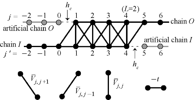
Figure 3: Schema of the reduced Hamiltonian when $L=2$.

As was shown in Ref. Datta ,

$$\left(\widetilde{g}_{\mu}\right)_{m,n}=\frac{-i}{\sqrt{3}t}\left(\,\omega^{(\mu)}\right)^{|\,m-n\,|}$$ (23)

where Eq. (13) was used. Using Dyson’s equation $g=\widetilde{g}+\widetilde{g}h_{c}g$, we can derive

$$\left(g_{O}\right)_{m,n}=\left(\widetilde{g}_{O}\right)_{m,n}+\left(\widetilde{g}_{O}\right)_{m,0}t\left(g_{O}\right)_{1,n}.$$ (24)

Substituting $m=1$ in Eq. (24),

$$\left(g_{O}\right)_{1,n}=\frac{\left(\widetilde{g}_{O}\right)_{1,n}}{1-t\left(\widetilde{g}_{O}\right)_{1,0}}$$ (25)

is obtained. Using Eqs. (23), (24) and (25),

$$\left(g_{O}\right)_{m,n}=\left(\widetilde{g}_{O}\right)_{m,n}-\left(\widetilde{g}_{O}\right)_{m+n,0}.$$ (26)

The matrix $g_{I}$ is obtained in the same way as

$$\left(g_{I}\right)_{m,n}=\left(\widetilde{g}_{I}\right)_{m,n}-\left(\widetilde{g}_{I}\right)_{m+n,4L+2}.$$ (27)

Dyson’s equations $\widetilde{G}=\widetilde{g}+\widetilde{g}\;V\widetilde{G}=\widetilde{g}\sum_{m}(V\;\widetilde{g})^{m}$ and $G=g+gVG=g\sum_{m}(Vg)^{m}$ indicate

$$\widetilde{G}_{j,j^{\;\prime}} = \left[\widetilde{g}_{O}\bar{V}\widetilde{g}_{I}\left(1-^{\;t}\!\bar{V}\widetilde{g}_{O}\bar{V}\widetilde{g}_{I}\right)^{-1}\right]_{j,j^{\;\prime}}$$ (28)

and

$$G_{j,j^{\;\prime}}=\left[g_{O}\bar{V}g_{I}\left(1-^{\;t}\!\bar{V}g_{O}\bar{V}g_{I}\right)^{-1}\right]_{j,j^{\;\prime}}$$ (29)

,respectively, where $\widetilde{G}_{j,j^{\;\prime}}\equiv\langle\langle O,j\,|\,\widetilde{G}\,|I^{\,},j^{\;\prime}\,\rangle\rangle$ and $G_{j,j^{\;\prime}}\equiv\langle\langle O,j\,|\,G\,|I^{\,},j^{\;\prime}\,\rangle\rangle$ . Using Fisher-Lee relationDatta ; Fisher-Lee and Eq. (13), we can obtain the transmission rate $T$ as

$$T=3t^{2}\left|\widetilde{G}_{2L+1,0}\right|^{2}$$ (30)

including the higher terms and

$$T=3t^{2}\left|G_{2L+1,0}\right|^{2}$$ (31)

including both the higher terms and reflection at the open edges. The explicit relation of Eq. (30) and Eq. (31) to the inter-chain elements $\bar{V}_{j,j^{\;\prime}}$ is summarized in the Appendix. In the Appendix, we can see that the first order term of Eq. (30), $3t^{2}|\left(\widetilde{g}_{O}\bar{V}\,\widetilde{g}_{I}\right)_{2L+1,0}|^{2}$, coincides with the FGR formula (14).

III.3 Expansion of Eq. (30)

Equation (30) can be expanded as

$$T=3t^{2}\left|\sum_{m=0}^{\infty}\left(\frac{-1}{3t^{2}}\right)^{m+1}q_{m}\right|^{2}$$ (32)

where

$$q_{m} \equiv (-3t^{2})^{m+1}\left(\widetilde{g}_{O}\bar{V}\,\widetilde{g}_{I}(^{\;t}\bar{V}\,\widetilde{g}_{O}\bar{V}\,\widetilde{g}_{I})^{m}\right)_{2L+1,0}$$ (33)

$$= \sum_{j_{l},j^{\prime}_{l},s_{l},s^{\prime}_{l}}e^{i(\beta_{O}+\beta_{I})}f$$

$$f=\bar{V}_{j_{m},j_{m}+s_{m}}\prod_{l=0}^{m-1}\bar{V}_{j_{l},j_{l}+s_{l}}\bar{V}_{j^{\prime}_{l}+s^{\prime}_{l},j^{\prime}_{l}}$$ (34)

$$\beta_{O}=\frac{k^{(O)}}{2}a\left(-j_{0}+\sum_{l=0}^{m-1}|j^{\prime}_{l}+s^{\prime}_{l}-j_{l+1}|\right)$$ (35)

and

$$\beta_{I}=\frac{k^{(I)}}{2}a\left(|j_{m}+s_{m}|+\sum_{l=0}^{m-1}|j_{l}+s_{l}-j^{\prime}_{l}|\right).$$ (36)

As the ranges of indexes of Eq. (33) are $1\leq j_{l}\leq 2L,\;1\leq j^{\prime}_{l}\leq 2L,\;-1\leq s_{l}\leq 1$ and $-1\leq s^{\prime}_{l}\leq 1$,note-index the number of terms in Eq. (33) is $3^{2m+1}(2L)^{2m+1}$. Firstly we consider the case of $\varepsilon=0$, i.e., $k^{(O)}=k^{(I)}$. Among the $3^{2m+1}(2L)^{2m+1}$ terms, those satisfying the condition

$$j_{0}>j^{\prime}_{0}>j_{1}>j^{\prime}_{1}>\cdots>j^{\prime}_{m-1}>j_{m}$$ (37)

are dominant, because $\beta_{O}+\beta_{I}=s_{m}+\sum_{l=0}^{m-1}(s_{l}+s^{\prime}_{l})$ irrespective of indexes $\{j_{l},j^{\prime}_{l}\}$ in these dominant terms. The other terms cancel each other because of their random phases $\beta_{O}+\beta_{I}$. Since the number of the dominant terms is $3^{2m+1}(2L)^{2m+1}/(2m+1)!$, Eq. (33) can be approximated by

$$q_{m}=\frac{L^{2m+1}}{(2m+1)!}A|A|^{2m}$$ (38)

where $A$ was defined by Eq. (16). From Eqs. (32) and (38), we can obtain

$$T=\sin^{2}\left(\frac{|A|L}{\sqrt{3}t}\right).$$ (39)

In order to discuss the case where $k^{(O)}\neq k^{(I)}$, we refer to the dispersion relation of the DWNT. The DWNT can be approximated by the double chain of which the inter-chain Hamiltonian element $V^{\prime}_{j,j^{\;\prime}}$ is related to Eq. (19) as $V^{\prime}_{j,j^{\;\prime}}\equiv(\bar{V}_{1,1+j^{\;\prime}-j}+\bar{V}_{2,2+j^{\;\prime}-j})/2$. The dispersion relation of the double chain is obtained as ref1 ; ref2

$$E^{(\pm)}_{\sigma,k}=E^{(I)}_{\sigma,k}+\frac{1}{2}\left(\varepsilon\pm\sqrt{\varepsilon^{2}+|\widetilde{A}_{\sigma}|^{2}}\right)$$ (40)

where

$$\widetilde{A}_{\sigma}\equiv\sum_{j=1}^{2}\sum_{s=-1}^{1}\bar{V}^{\sigma,\sigma}_{j,j+s}\exp(ikas/2).$$ (41)

Figure 4 shows that Eq. (40) coincides well with the exact dispersion lines. Comparing Eq. (41) with Eq. (16), we can see that $\widetilde{A}_{\sigma}$ and $A_{\sigma,\sigma}$ are essentially the same. In Eq. (40), we can see that the intrinsic band shift $\varepsilon$ changes the total band shift $E^{(+)}-E^{(-)}$ from $|A|$ to $\sqrt{|A|^{2}+\varepsilon^{2}}$. Assuming the same effect of $\varepsilon$ on Eq. (38), we can obtain

$$q_{m}=\frac{L^{2m+1}}{(2m+1)!}A(|A|^{2}+\varepsilon^{2})^{m}.$$ (42)

From Eqs. (32) and (42), we can also obtain

$$T=\frac{|A|^{2}}{|A|^{2}+\varepsilon^{2}}\sin^{2}\left(\frac{L\sqrt{|A|^{2}+\varepsilon^{2}}}{\sqrt{3}t}\right).$$ (43)

When $L\sqrt{|A|^{2}+\varepsilon^{2}}\ll\sqrt{3}t$ or $|A|\ll|\varepsilon|$, Eq. (43) coincides with Eq. (21).

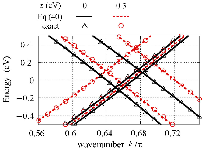
Figure 4: The dispersion relation of the DWNT with parameters $(n_{O},n_{I},\Delta\theta,\Delta z)=(10,5,\frac{4\pi}{130},-0.05a)$ and $\varepsilon$ (eV) =0, 0.3. The triangles and circles show the exact dispersion relation. The solid and dashed lines represent Eq. (40).

IV Analysis with the perturbation formula

In the following sections, the transmission rates at $E_{F}=0.1$ eV $\simeq 0.0364t$ are calculated from the conditioned transfer matrix (CTM) Tamura ; Tamura-CTM and the perturbation formulas (20),(30),(31) with the common TB Hamiltonian. In the CTM, the transmission rates were obtained from the $S$ (scattering) matrix and the numerical errors were estimated to be $\sum_{i,k}|(\sum_{j}S^{*}_{j,i}S_{j,k})-\delta_{i,k}|$, as the exact $S$ matrix must be unitary. The estimated errors of the CTM in this paper were less than $4\times 10^{-6}$. Though the perturbation results were less accurate than the CTM results, they are useful in analyzing the CTM results.

IV.1 Original TB model ( $\varepsilon=0$, $r_{c}=0.39085$ nm)

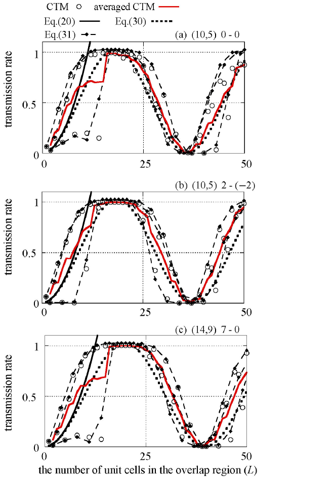
Figure 5: Interlayer transmission rates $T_{+,+}$ between the $+$ channels of $(n_{O},n_{I})$ $i_{\theta}$-$i_{z}$ TDWNTs at $E_{F}=0.1$ eV, where $\Delta\theta=2\pi i_{\theta}/(13n_{O})$ and $\Delta z=ai_{z}/40$. The black solid lines, dotted lines, closed diamonds, open circles and red solid lines show Eqs. (20), (30), (31), CTM and averaged CTM, respectively. The closed diamonds are connected with the dashed lines at intervals of $3a$. The values of $|A_{+,+}|/t$ are 0.1492, 0.1435 and 0.1355 in (a), (b) and (c), respectively.

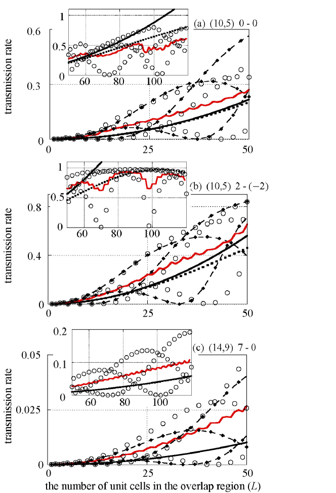
Figure 6: The same calculations as in Fig. 5, except the transmissions $T_{-,-}$ are between the $-$ channels. In (c), Eq. (20) and Eq. (30) nearly coincide with each other. In the insets with the range $50\leq L\leq 120$, the data of Eq. (31) are omitted because they make the insets busy. The values of $|A_{-,-}|/t$ are 0.0167, 0.0262 and 0.0036 in (a), (b) and (c), respectively.

Figures 5 and 6 represent $T_{+,+}$ and $T_{-,-}$, respectively, as a function of integer $L$. The overlap length $(L-0.5)a-\Delta z$ was changed discretely and $\Delta z$ was fixed. The black solid lines, dotted lines, closed diamonds and open circles show Eqs. (20), (30), (31), and CTM, respectively. In contrast to the monotonic increase of FGR formula (20) with $L$, CTM and Eq. (31) showed a rapid oscillation with a period close to $3a$ superimposed on a slower oscillation. Only a slower oscillation appeared in Eq. (30) because Eq. (30) does not include the reflection at the open edge. To show the slower oscillation, the closed diamonds were connected with the dashed lines at intervals of $3a$ and the averaged CTM data defined as $T^{(ave)}_{L}=(T_{L-1}+T_{L}+T_{L+1})/3$ were shown by the red solid lines.

The effects of the structure parameters ($L,n_{O},\Delta z,\Delta\theta$ ) were reproduced qualitatively by the first order formula (20) when Eq. (20) is less than unity, i.e., when $L<\sqrt{3}t/|A|$. The values of $|A|/t$ are shown in Figure captions. Even when $L>\sqrt{3}t/|A|$, Eqs. (30) and (31), which include higher order terms, were effective, indicating the validity of the perturbation formula. Note the scale of the vertical axis in Fig. 6. The transmission rate $T_{-,-}$ of the TDWNTs becomes larger particularly when $n_{O}=n_{I}+5=10$. Tamura

IV.2 Modification of $r_{c}$

When $n_{O}=n_{I}+5=10$, the maximum conductance of the TDWNT is $2G_{0}$ in the tight-binding (TB) calculation, but only $G_{0}$ in the local density approximation (LDA) .Tamura ; telescope-Kim ; telescope-Buia ; telescope-comp-phys ; Kim The difference in the interlayer Hamiltonian between TB and LDA is the most probable origin of this disagreement. To evaluate the order of the interlayer Hamiltonian elements in the LDA calculation, the ADF calculation ADF1 ; ADF2 ; ADF3 with single zeta 1s, 2s, and 2p orbitals was performed for a (10,10)-(5,5) DWNT composed of four unit cells. The structure is represented by Eq. (1), $1\leq j\leq 8$, $\Delta\theta=0$, and $\Delta z=0.025a$. Dangling bonds at $j=1,8$ were terminated by hydrogen atoms with a bond length of 0.11 nm. In the $(R_{\mu}\theta,z)$ plane, the C-C-H angle is $2\pi/3$ as is the C-C-C angle. Geometric optimization was omitted, since a slight change in the structure is not relevant to the order of the interlayer elements. With the $\pi$ orbital $\psi_{\pi}$ defined as $\psi_{\pi}\equiv\cos\theta\phi_{2{\rm px}}+\sin\theta\phi_{2{\rm py}}$, Fig. 7 shows the interlayer ADF Fock matrix elements of the $\pi$ orbitals as a function of atomic distance. The TB elements used in Ref.Tamura are also shown in Fig. 7 for comparison. The intralayer elements between nearest neighbors were $-4.73\sim-4.49$ eV in the ADF and $-t=-2.75$ eV in the TB. Thus, Fig. 7 shows that the interlayer elements normalized by the nearest neighbor elements were larger in the ADF than in the TB model. When we adjust the TB model to reproduce the LDA results, the adjusted TB model needs to have contradictory features; larger interlayer elements and smaller interlayer transmission rates compared to the original TB. To resolve the contradiction, we should notice that the ADF result showed no clear cutoff radius $r_{c}$ in Fig. 7. Inspired by these results, we discuss the effect of $r_{c}$ in this section.

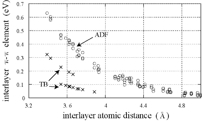
Figure 7: Interlayer Fock matrix elements between $\pi$ orbitals calculated by ADF. Interlayer tight-binding model based on Ref.Lambin is shown as crosses for comparison.

Figure 8 shows $T_{-,-}$ for $r_{c}=0.385$ nm, 0.39085 nm and 0.4 nm. We can see that $T_{-,-}$ increases as $r_{c}$ decreases in the averaged CTM results (dotted lines). As this relation between $r_{c}$ and $T_{-,-}$ was reproduced by the perturbation formulas (solid lines and dashed lines), it can be explained by the effective interlayer interaction $A_{-,-}$ as follows. Interlayer bonds are drawn between atoms $(O,l,1)$ and $(I,l^{\;\prime},2)$ in Fig. 9 when the corresponding Hamiltonian elements $\langle O,l,1|V|I,l^{\;\prime},2\,\rangle$ are finite, or when the atomic distances are smaller than $r_{c}$. The interlayer bonds with even or odd $l+l^{\;\prime}$ are called even or odd bonds in the following discussion, and represented by solid or dashed lines, respectively, in Fig. 9, where the parity of $l$ and $l^{\;\prime}$ is distinguished by triangles and circles, using the same representation of parity as in Fig. 2.

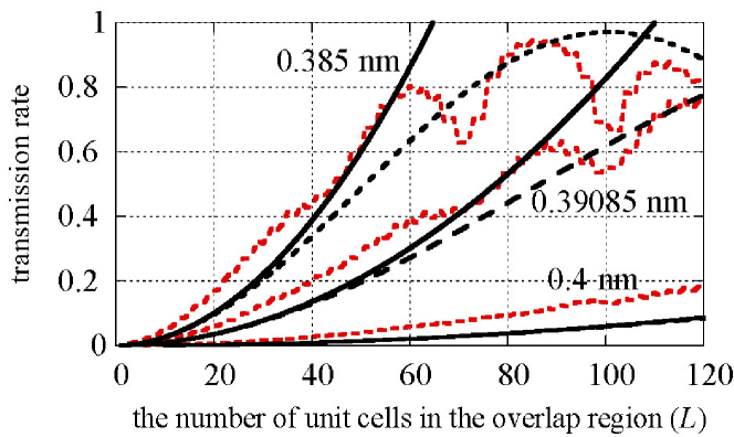
Figure 8: Interlayer transmission rate $T_{-,-}$ of the TDWNT ($n_{O}=n_{I}+5=10,\Delta\theta=4\pi/130,\Delta z=0$) calculated at $E_{F}=0.1$ eV using Eq. (20) (solid lines), Eq. (30) (dashed lines) and the averaged CTM (dotted lines) for the shortened cutoff radius $r_{c}=0.385$ nm, the original one $r_{c}=0.39085$ nm and the lengthened one $r_{c}=0.4$ nm. The values of $|A_{-,-}|/t$ are 0.0271, 0.0160 and 0.0044 when $r_{c}=0.385$ nm, 0.39085 nm and 0.4 nm, respectively.

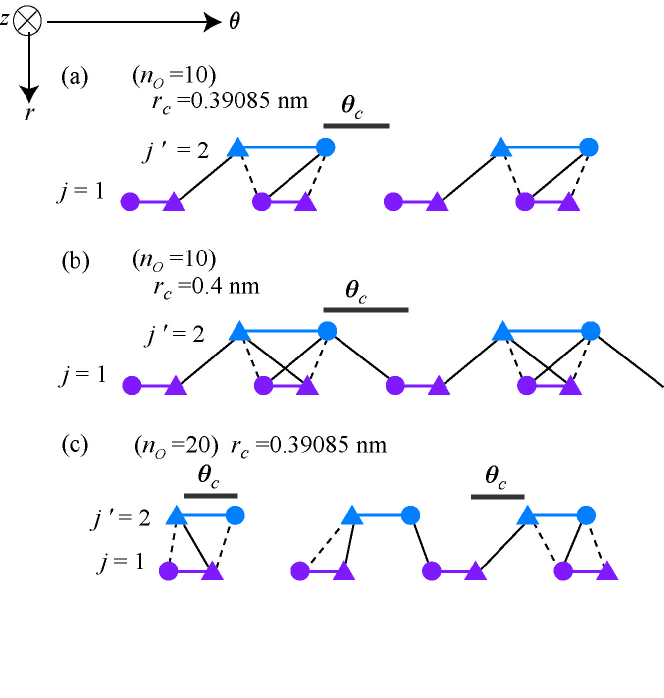
Figure 9: Horizontal positions of triangles and circles indicate $\theta$ coordinates of atoms $(O,l,1)$ and $(I,l^{\;\prime},2)$ (a), (b) $n_{O}=n_{I}+5=10,\Delta\theta=4\pi/130,\Delta z=0$, and (c) $n_{O}=n_{I}+5=20,\Delta\theta=-\pi/60,\Delta z=0$. The interlayer bonds were drawn when the inter-atomic distance was smaller than $r_{c}$, so that the corresponding Hamiltonian elements shown by Eq. (2) were finite. The cutoff radius $r_{c}$ was 0.39085 nm in (a) and (c), and 0.4 nm in (b). The interlayer bond between atoms $\alpha$ and $\beta$ was formed only when $|\theta_{\alpha}-\theta_{\beta}|<\theta_{c}\equiv 2\arcsin\left(\sqrt{(4\pi^{2}r_{c}^{2}-X))/(12n_{I}n_{O}a^{2})}\;\right)$. Here $X\equiv(75+\pi^{2}(j^{\;\prime}-j)^{2})a^{2}$, $j^{\;\prime}-j=2-1=1$, and $\theta_{c}$ is shown by bars.

Figure 10: Changes of $|A_{-,-}|^{2}$ of the (10,10)-(5,5) TDWNTs caused by increase of $r_{c}$ from 0.39085 nm to 0.4 nm. The interlayer configurations are $\Delta\theta=i_{\theta}\pi/65$ $(i_{\theta}=0,1,2,\cdots,12)$ and $\Delta z=i_{z}a/40$ $(i_{z}=0,1,2,3,4)$.

The parameters ( $n_{O},\Delta\theta,\Delta z$) were chosen to be the same in Figs. 9 (a) and (b) as in Fig. 8. Since $T_{-,-}$ in Eq. (20) is reduced by different parities of $l+l^{\;\prime}$ in Eq. (19), the reduction of $T_{-,-}$ is determined by the balance between odd and even bonds. This balance tends to be lost when the number of interlayer bonds per unit cell is small, as is illustrated by Fig. 9 (a); the even bonds are considerably longer than the odd bonds, although they are equal in number. On the contrary, this imbalance is redressed in Fig. 9 (b) by increase of the number of interlayer bonds caused by increasing $r_{c}$. In cases where $n_{O}>10$, on the other hand, the number of interlayer bonds is large enough to reduce $T_{-,-}$ without increasing $r_{c}$. This is illustrated in Fig. 9 (c), where $n_{O}=n_{I}+5=20,$ $\Delta\theta=-\pi/60$, and $\Delta z=0$. Figure 10 shows $|A_{-,-}(r_{c}=0.4{\rm nm})|^{2}-|A_{-,-}(r_{c}=0.39085{\rm nm})|^{2}$ for the (10,10)-(5,5) TDWNTs of which the interlayer configurations are $\Delta\theta=i_{\theta}\pi/65$ $(i_{\theta}=0,1,2,\cdots,12)$ and $\Delta z=i_{z}a/40$ $(i_{z}=0,1,2,3,4)$. Figure 10 clearly indicates that increase of $r_{c}$ tends to reduce $|A_{-,-}|^{2}$ and $T_{-,-}$.

IV.3 Modification of $\varepsilon$

Figure 6 of Ref. Kim indicates a close correlation between the intrinsic band shift $|\varepsilon|$ and the suppression of the transmission rate $T_{-,-}$. These appeared in multi-band TB multiband-TB ; multiband-TB-okada ; Slater and LDA, but not in single band TB. Here we should distinguish $|\varepsilon|$ from the total shift $\sqrt{|A|^{2}+\varepsilon^{2}}$ shown by Eq. (40). Inspired by these results, we investigate the effects of $|\varepsilon|$ in this section.

Figures 11 and 12 show the same calculations as Figs. 5 (b) and 6 (b), respectively, except that the intrinsic band shift $\varepsilon$ was changed from zero to (a) 0.1 eV (b) 0.3 eV, or (c) 0.5 eV. The decrease in the CTM transmission rate with increasing $\varepsilon$ was reproduced qualitatively by Eq. (20). We can also see that precision of the perturbation formula was systematically improved by Eqs. (30) and (31).

Equation (30) almost coincides with Eq. (43) as is seen in Fig. 13. Thus Eq. (43) indicates that the first peak of Eq. (30) as a function of $L$ appears at

$$(L,T)=\left(\frac{t\sqrt{3}\pi}{2\sqrt{|A|^{2}+\varepsilon^{2}}},\;\frac{|A|^{2}}{|A|^{2}+\varepsilon^{2}}\right).$$ (44)

The first peak position of the averaged CTM is denoted by $(L_{\rm ctm},\;T_{\rm ctm})$ and compared to Eq. (44) in Table I for Figs. 5 (b), 6 (b), 11 and 12. The peak height of Eq. (44) is lower than $T_{\rm ctm}$ when $|\varepsilon|/|A|$ is large. Nevertheless Eq. (44) qualitatively reproduces the dependence of $(L_{\rm ctm},\;T_{\rm ctm})$ on $\varepsilon$. When $|\varepsilon|\ll t$, the intrinsic shift $\varepsilon$ exercises only slight influence over $|A|$.

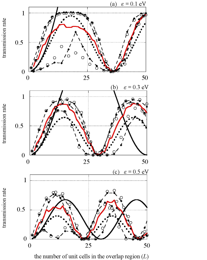
Figure 11: The same calculations as in Fig. 5 (b), except the intrinsic band shift $\varepsilon$ was (a) 0.1 eV, (b) 0.3 eV, or (c) 0.5 eV. The values of $|A_{+,+}|/t$ are shown in Table I.

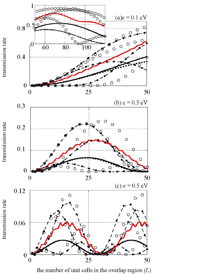
Figure 12: The same calculations as in Fig. 6 (b), except the intrinsic band shift $\varepsilon$ was (a) 0.1 eV, (b) 0.3 eV, or (c) 0.5 eV. The values of $|A_{-,-}|/t$ are shown in Table I.

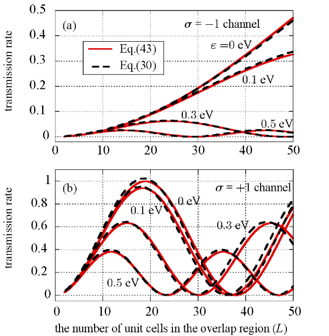
Figure 13: Comparison between Eq. (30) (dashed lines) and Eq. (43) (solid lines) when $(n_{O},n_{I},\Delta\theta,\Delta z)=(10,5,\frac{4\pi}{130},-0.05a)$ and $\varepsilon$ (eV) =0, 0.1, 0.3, 0,5. We can see that Eq. (30) almost coincides with Eq. (43). The data of Eq. (30) are shown also in Figs. 5(b), 6(b), 11 and 12.

$\varepsilon\;$(eV)		0	0.1	0.3	0.5
	$|A_{+,+}|/t$	0.1435	0.1435	0.1432	0.1430
	$\frac{\sqrt{3}t\pi}{2\sqrt{|A_{+,+}|^{2}+\varepsilon^{2}}}$	18.95	18.38	15.11	11.76
$\sigma=+1$	$(L_{\rm ctm})$	(18)	(15)	(13)	(14)
	$\frac{|A_{+,+}|^{2}}{|A_{+,+}|^{2}+\varepsilon^{2}}$	1.000	0.940	0.633	0.382
	($T_{\rm ctm})$	(0.998)	(0.807)	(0.873)	(0.570)
	$|A_{-,-}|/t$	0.0262	0.0268	0.0279	0.0291
	$\frac{\sqrt{3}t\pi}{2\sqrt{|A_{-,-}|^{2}+\varepsilon^{2}}}$	103.9	60.25	24.16	14.78
$\sigma=-1$	$(L_{\rm ctm})$	(90)	(70)	(28)	(16)
	$\frac{|A_{-,-}|^{2}}{|A_{-,-}|^{2}+\varepsilon^{2}}$	1.000	0.351	0.062	0.025
	($T_{\rm ctm})$	( 0.918)	(0.787)	(0.149)	(0.061)

Table 1: The first peak positions of the averaged CTM $(L_{\rm ctm},T_{\rm ctm})$ in Figs. 5 (b), 6 (b), 11 and 12 are compared with Eq. (44). The values of $|A|/t$ are also shown.

V summary and discussion

Considering the interlayer Hamiltonian as a perturbation, we derived the first order formula (20), the formula including the higher-order terms (30), the formula including both the higher-order terms and reflection at the open edges (31). Expanding Eq. (30), we can see that Eq. (30) is the essentially the same as Eq. (43). They were applied to TDWNTs composed of $(n_{O},n_{O})$ and $(n_{O}-5,n_{O}-5)$ armchair tubes.

The perturbation formulas clarified the effects of the interlayer Hamiltonian on the interlayer conductance $G$. The product of the interlayer Hamiltonian and the wave function can be considered as the effective interlayer interaction because it determines the perturbation formulas (20), (43) and the dispersion relation (40). The effective interlayer interaction per unit cell and that per total overlapped region were denoted by $A_{\sigma,\sigma^{\;\prime}}$ and $A_{\sigma,\sigma^{\;\prime}}B_{\sigma,\sigma^{\;\prime}}$, respectively. Here the parity $\sigma=+,-$ or $\sigma^{\;\prime}=+,-$ indicates whether the wave function of the outer or inner tube, respectively, changes its sign along the circumference. The first order (FGR) formula (20) was proportional to $|A_{\sigma,\sigma^{\;\prime}}|^{2}|B_{\sigma,\sigma^{\;\prime}}|^{2}$. Because $|B_{\sigma,-\sigma}|$ was negligible compared to $|B_{\sigma,\sigma}|$, we could neglect the inter-channel transmission rates $T_{+,-}$ and $T_{-,+}$.

The CTM transmission rate had a rapid oscillation superimposed on a slower oscillation as a function of $L$. Although Eqs. (20) and (30) could not reproduce the rapid oscillation, they approximated the long-period oscillation. The rapid oscillation is reproduced by Eq. (31), which includes the reflection at the open edge. The first order formula (20) exceeds unity when $|\varepsilon|<|A|$, while the higher-order formula (30) never exceeds unity and reproduced qualitatively the first peak of the CTM results. The systematic improvement of the accuracy indicates the validity of the perturbation formulas.

To represent the range $L<L_{max}$ where Eq. (20) reproduced the averaged CTM results, we define $L_{1}\equiv t\sqrt{3}/|A|$ and $L_{2}\equiv\pi t\sqrt{3}/\sqrt{4|A|^{2}+4\varepsilon^{2}}$; Equation (22) reaches unity at $L=L_{1}$ and the first peak of Eq. (30) appears at $L=L_{2}$. The upper limit of the effective range, $L_{max}$, is classified according to $|\varepsilon|/|A|$ as follows. (i) When $|\varepsilon|/|A|\gg 1$, Eq. (20) almost coincided with Eq. (30) and showed the underestimated peak heights. Nevertheless it reproduced well the period of the oscillation of the averaged CTM even when $L>L_{2}$. In this sense, $L_{max}>L_{2}$. Figures 12 (b) and 12 (c) correspond to this case. (ii)$L_{max}=L_{2}(<L_{1})$ when $|\varepsilon|/|A|$ is comparable to unity but larger than $\sqrt{\frac{\pi^{2}}{4}-1}(\simeq 1.2)$. Figures 11 (c) and 12 (a) correspond to this case. (iii)$L_{max}=L_{1}(<L_{2})$, when $|\varepsilon|/|A|<\sqrt{\frac{\pi^{2}}{4}-1}$. Figures 5,6, 8, 11 (a) and 11 (b) correspond to this case.

Since the first principle results suggested the significant effects of the cutoff radius $r_{c}$ and the intrinsic band shift $\varepsilon$ on the conductance, they were analyzed by the effective interlayer interaction $A_{\sigma,\sigma}B_{\sigma,\sigma}$ in Eq. (20). The band shift $|\varepsilon|$ reduced the conductance because it lowered $|B|$. As $r_{c}$ became longer, the number of nonzero terms in Eq. (19) increased. When $\sigma=\sigma^{\;\prime}=-$, the nonzero terms introduced by increasing $r_{c}$ could cancel the terms already present in Eq. (19). Thus, a longer $r_{c}$ could reduce $|A_{-,-}|$ and $T_{-,-}$.

In contrast to rigorous calculations, which involve complicated matrix inversion, the first order perturbation formula (20) involves a simple linear combination of the interlayer Hamiltonian elements. This enabled us to clarify the role of the interlayer Hamiltonian in the transmission rate. In addition to DWNTs, there are various other systems composed of two monolayer subsystems; side-to-side contact of two SWNTs, AFM-sidecontact-SWNTbridge ; telescope-Buia ; Turnney-Cooper an SWNT on graphene, NT-on-graphene and bilayer graphene. few-layer-graphite By sliding one subsystem along the other, a generalized telescoped system can be obtained in which the interlayer bonds can be considered a perturbation. The perturbation formula is an important tool to analyze the NEMS formed by these telescoped systems.

*

Appendix A

Eqs. (30) and (31) are explicitly related to Eq. (19) in this Appendix. Only the case where $\sigma=\sigma^{\;\prime}$ is considered here and thus index $\sigma$ is suppressed in the following formulas as in Sec. III B. For example, the symbol $\bar{V}^{\sigma,\sigma}_{j,j^{\;\prime}}$ is abbreviated as $\bar{V}_{j,j^{\;\prime}}$.

Eqs. (30) and (31) can be represented by

$$3t^{2}\left|\widetilde{G}_{2L+1,0}\right|^{2}=\left|\sum\limits_{j^{\,\prime}=0}^{2L}\widetilde{x}_{j^{\,\prime}}\widetilde{Y}_{j^{\,\prime},\,0}\right|^{2}$$ (45)

and

$$3t^{2}\left|G_{2L+1,0}\right|^{2}=\left|\sum\limits_{j^{\,\prime}=0}^{2L}x_{j^{\,\prime}}Y_{j^{\,\prime},\,0}\right|^{2}$$ (46)

with the following formulas

$$\widetilde{x}_{j^{\,\prime}} \equiv -\sqrt{3}t\left(\omega^{(O)}\right)^{-2L-1}\left(\widetilde{g}_{O}\bar{V}\widetilde{g}_{I}\right)_{2L+1,j^{\,\prime}}$$ (47)

$$= \sum_{j_{0}=1}^{2L+1}\left(\omega^{(O)}\right)^{-j_{0}}v_{j_{0},j^{\,\prime}}^{(I)},$$

$$\widetilde{Y}=\left(1+v^{(O)}v^{(I)}\right)^{-1},$$ (48)

$$v^{(I)}_{j,j^{\,\prime}} \equiv i(\bar{V}\widetilde{g}_{I})_{j,j^{\,\prime}}$$ (49)

$$= \sum_{s=-1}^{1}\frac{\bar{V}_{j,j+s}}{\sqrt{3}t}\left(\omega^{(I)}\right)^{|j+s-j^{\;\prime}|},$$

$$v^{(O)}_{j^{\,\prime},j} \equiv i(\,^{t}\bar{V}\widetilde{g}_{O})_{j^{\,\prime},j}$$ (50)

$$= \sum_{s^{\;\prime}=-1}^{1}\frac{\bar{V}_{j^{\;\prime}+s^{\;\prime},j^{\;\prime}}\;}{\sqrt{3}t}\left(\omega^{(O)}\right)^{|j^{\;\prime}+s^{\;\prime}-j|},$$

$$x_{j^{\,\prime}} \equiv -i\sqrt{3}t\left(\omega^{(O)}\right)^{-2L-1}\left(g_{O}\bar{V}g_{I}\right)_{2L+1,j^{\,\prime}}$$ (51)

$$= \sum_{j=1}^{2L+1}2\sin\left(\frac{k^{(O)}a}{2}j\right)X_{j,j^{\,\prime}}^{(I)},$$

$$Y=(1+X^{(O)}X^{(I)})^{-1},$$ (52)

$$X_{j,j^{\,\prime}}^{(I)}=v_{j,j^{\,\prime}}^{(I)}-v_{j,4L+2-j^{\,\prime}}^{(I)},$$ (53)

and

$$X_{j^{\,\prime},j}^{(O)}=v_{j^{\,\prime},j}^{(O)}-v_{j^{\,\prime},-j}^{(O)}\;\;.$$ (54)

For the inverse matrix calculation in Eqs. (48) and (52), $v^{(\mu)}$ and $X^{(\mu)}$ are considered as $(2L+1)\times(2L+1)$ matrixes in which indexes are restricted to $1\leq j\leq 2L+1$ and $0\leq j^{\;\prime}\leq 2L$. From Eqs. (47), (48), (49) and (50), we can obtain Eqs. (32), (33), (34), (35) and (36). Eqs. (47) and (49) show that the first order term of Eq. (30), $3t^{2}|\left(\widetilde{g}_{O}\bar{V}\,\widetilde{g}_{I}\right)_{2L+1,0}|^{2}=|\widetilde{x}_{0}|^{2}$, coincides with the FGR formula (14).

References

- (1) N. Hamada, S. I. Sawada, and A. Oshiyama, Phys. Rev. Lett. 68, 1579 (1992); J. W. Mintmire, B. I. Dunlap, and C. T. White, ibid 68, 631 (1992); R. Saito, M. Fujita, G. Dresselhaus, and M. S. Dresselhaus, Phys. Rev. B 46, 1804 (1992).
- (2) R. Saito, G. Dresselhaus, and M. S. Dresselhaus, Physical Propertiesof Carbon Nanotubes (Imperial College Press, London,1998).
- (3) J. -C. Charlier, X. Blase, and S. Roche, Rev. Mod. Phys. 79, 677 (2007).
- (4) P. Tangney, M. L. Cohen, and S. G. Louie, Phys. Rev. Lett. 97, 195901 (2006).
- (5) J. Servantie and P. Gaspard, Phys. Rev. B 73, 125428 (2006); Phys. Rev. Lett. 91 185503 (2003).
- (6) E. Bichoutskaia, A. M. Popov, A. El-Barbary, M. I. Heggie, and Y. E. Lozovik, Phys. Rev. B 71, 113403 (2005). E. Bichoutskaia, M. I. Heggie, A. M. Popov, and Y. E. Lozovik, ibid. 73, 045435 (2006).
- (7) Q. Zheng and Q. Jiang, Phys. Rev. Lett. 88 045503 (2002). S. B. Legoas, V. R. Coluci, S. F. Braga, P. Z. Coura, S.O. Dantas, and D. S. Galvao, ibid. 90 055504 (2003). W. Guo, Y. Guo, H. Gao, Q. Zheng and W. Zhong. ibid 91, 125501 (2003); Q. Zheng, J. Z. Liu and Q. Jiang, Phys. Rev. B 65, 245409 (2002).
- (8) R. Saito, M. Matsumoto, T. Kimura, G. Dresselhaus and M. S. Dresselhaus, Chem. Phys. Lett. 348, 187 (2001).
- (9) B. Bhushan, X. Ling, A. Jungen and C. Hierold, Phys. Rev. B 77 165428 (2008). B. Bhushan and X. Ling, ibid. 78 045429 (2008).
- (10) K. Jensen, C. Girit, W. Mickelson, and A. Zettl, Phys. Rev. Lett. 96 215503 (2006).
- (11) A. Kis, K. Jensen,S. Aloni, W. Mickelson, and A. Zettl, Phys. Rev. Lett. 97 025501 (2006).
- (12) J. Cumings and A. Zettl, Science 289, 602 (2000); Phys. Rev. Lett. 93, 086801 (2004).
- (13) S. Akita and Y. Nakayama, J. J. Appl. Phys. 43, 3796 (2004).
- (14) Q. Yan, G. Zhou, S. Hao, J. Wu, and W. Duan, Appl. Phys. Lett. 88, 173107 (2006).
- (15) The effective interlayer interaction was denoted by in Ref.Tamura . When , Eq. (40) coincides with Eq. (23) of Ref.Tamura , where and .
- (16) R. Tamura, Y. Sawai, and J. Haruyama, Phys. Rev. B 72, 045413 (2005).
- (17) S. Uryu and T. Ando, Phys. Rev. B 76, 155434 (2007).
- (18) D. -H. Kim and K. J. Chang, Phys. Rev. B, 66, 155402 (2002).
- (19) C. Buia, A. Buldum, and J. P. Lu, Phys. Rev. B, 67, 113409 (2003).
- (20) Y. -J. Kang, J. Kang, Y, -H Kim, K. J. Chang, Comp. Phys. Commun. 177 30 (2007).
- (21) Y-J. Kang, K. J. Chang, and Y H. Kim, Phys. Rev. B 76, 205441 (2007).
- (22) A. Hansson and S. Stafstrom, Phys. Rev. B, 67, 075406 (2003).
- (23) I. M. Grace, S. W. Bailey, and C. J. Lambert, Phys. Rev. B, 70, 153405 (2004).
- (24) S. Uryu and T. Ando, Phys. Rev. B 72, 245403 (2005).
- (25) M. A. Tunney and N. R. Cooper, Phys. Rev. B 74, 075406 (2006).
- (26) Ph. Lambin, V. Meunier, and A. Rubio, Phys. Rev. B 62, 5129 (2000).
- (27) J. C. Charlier, J. P. Michenaud, and Ph. Lambin, Phys. Rev. B 46, 4540 (1992).
- (28) Five significant figures of and were necessary to reproduce the results of Ref.Tamura , because and cause a discontinuous change. In more realistic calculations, we should replace this by a continuous change.
- (29) Y. -K. Kwon and D. Tománek, Phys. Rev. B 58, R16001 (1998); Y. Miyamoto, S. Saito, and D. Tománek, ibid 65, 041402 (2001). R. Saito, G. Dresselhaus, and M. S. Dresselhaus, J. Appl. Phys. 73, 494, (1993).
- (30) M. Pudlak and R. Pincak, Eur. Phys. J. B 67, 565 (2009).
- (31) Supriyo Datta, Electronic Transport in Mesoscopic Systems (Cambridge University Press, Cambridge 1995).
- (32) D. S. Fisher and P. A. Lee, Phys. Rev. B 23, 6851 (1981).
- (33) As we neglected in Eq. (14), the boundary corrections are neglected in Eq.(33). In the original definition, and . In Eq.(33), and . Here the element is the same as the original definition. Figure 3 illustrates the original definition of .
- (34) When Eq. (12) holds, the group velocity of Eq. (40) is positive. Using the relation and Eq. (40), we can obtain the linear dispersion line with the negative velocity in Fig. 4.
- (35) R. Tamura and M. Tsukada, Phys. Rev. B 61, 8548 (2000).
- (36) G. te Velde, F.M. Bickelhaupt, S.J.A. van Gisbergen, C. Fonseca Guerra, E.J. Baerends, J.G. Snijders, T. Ziegler, ’Chemistry with ADF’, J. Comput. Chem. 22, 931 (2001).
- (37) C. Fonseca Guerra, J.G. Snijders, G. te Velde, and E.J. Baerends, Theor. Chem. Acc. 99, 391 (1998).
- (38) ADF2008.01, SCM, Theoretical Chemistry, Vrije Universiteit, Amsterdam, The Netherlands, http://www.scm.com.
- (39) M. S. Tang, C. Z. Wang, C. T. Chan, and K. M. Ho, Phys. Rev. B 53, 979 (1996).
- (40) S. Okada and S. Saito, J. Phys. Soc. Jpn. 64, 2100 (1995).
- (41) J. C. Slater and G. F. Koster, Phys. Rev. 94, 1498 (1954).
- (42) M. R. Falvo, J. Steele, R. M. Taylor II, and R. Superfine, Phys. Rev. B 62 R10665 (2000); A. Buldum and Jian Ping Lu, Phys. Rev. Lett. 83 5050 (1999).
- (43) K. S. Novoselov, A. K. Geim, S. V. Morozov, D. Jiang, Y. Zhang, S. V. Dubonos, I. V. Grigorieva, A. A. Firsov, Science 306, 666 (2004).