Feshbach Resonance Induced Fano Interference in Photoassociation

Abstract

We consider photoassociation from a state of two free atoms when the continuum state is close to a magnetic field induced Feshbach resonance and analyze Fano interference in photoassociation. We show that the minimum in photoassociation profiles characterized by the Fano asymmetry parameter $q$ is independent of laser intensity, while the maximum explicitly depends on laser intensity. We further discuss the possibility of nonlinear Fano effect in photoassociation near a Feshbach resonance.

I introduction

In recent times, quantum interferences have occupied a prominent place in physics and these occur rather ubiquitously. Many well-known examples of these include Fano interferences Fano61 ; eberly ; gsafano , electromagnetically induced transparency (EIT) EITHarrisPRL89 , vacuum induced interferences in spontaneous emission viiGSAbook . The quantum interferences have resulted in large number of applications in coherent control of the optical properties, control of spontaneous emission scullyzhuzubairyScience and slow light HauHarris ; recentpaperBoyd . Quantum interference has been experimentally demonstrated in coherent formation of molecules atom-molecule and Autler-Townes splitting two-photon ; moal in two-photon PA. Theoretical formulation of PA within the framework of Fano’s theory has been developed in Refs. semian and semian2 . Recent experimental Junker:prl:2008 ; Winkler ; ni and theoretical Mackie:prl:2008 ; pellegrini:njp:2009 ; cote2 ; Kuznetsova studies on photoassociation (PA) near a magnetic field Feshbach resonance (MFR) mfr have generated a lot of interest in Fano interference with ultracold atoms. In a remarkable experiment, Junker et al. Junker:prl:2008 have demonstrated asymmetric spectral line shape and saturation in PA due to a tunable MFR. Asymmetric line shape is a hallmark of Fano-effect and the experimental results of Junker:prl:2008 can be attributed to the Fano interference.

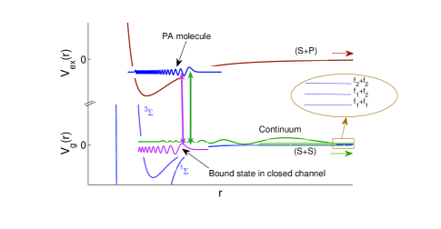
Figure 1: A Schematic diagram showing the diatomic potentials, continuum and bound states, bound-bound and bound-continuum laser couplings. Note that the two double-arrow vertical lines refer to the same laser field - green line corresponds to continuum-bound and the magenta line refers to bound-bound couplings. The ground asymptotic channels ($f_{a}+f_{b}$) in the absence of a magnetic field corresponds to separated atoms in two different hyperfine numbers $f_{a}$ and $f_{b}$.

Here we demonstrate quantum interference in the context of photoassociation (PA) pa under the condition when a Feshbach resonance is also involved in photoassociation. We show Fano like interference minimum in photoassociation spectrum. In analogy to the well know Fano q-parameter we can introduce a parameter which governs the existence of this minimum. Although the minimum is independent of laser intensity, the maximum is shown to depend explicitly on laser intensity. From our calculations we extract line shapes which are in broad agreement with the experimental results of junker et al. Junker:prl:2008 . Our formula for photoassociation is expressed in terms of parameters each of which has a clear physical meaning and is measurable. We derive probability of PA excitation for arbitrary intensities of the laser field and thus we also discuss nonlinear Fano effect. The current work has some features in common with the recent paper of Kuznetsova et al. Kuznetsova though these authors address a different problem which is the population transfer using two laser beams. Our emphasis is on quantum interferences in PA using a single laser beam.

The paper is organized in the following way. In section 2, we consider a simple model of three-channel time-independent scattering in the presence of an optical and a magnetic field. By using Green’s functions, we present compact analytical solution of the model. We then discuss selective results in Sec.3. The paper is concluded in Sec.4.

II The model and its solution

To begin with, we model PA in the presence of a Feshbach resonance as a three-channel scattering problem. There are two ground-state asymptotic hyperfine channels of which one is closed and the other one is open. The third channel corresponds to the photoassociated excited molecular configuration. The two ground state channels are coupled via hyperfine interaction. At a Feshbach resonance, the two atoms will form a quasibound state in the closed channel as schematically illustrated in Fig.1. As the strength of the applied magnetic field is varied, this quasibound state can move across the collision energy. When a PA laser is applied to form an excited photoassociated molecule (PM), there arise two competing pathways of dipole transitions as shown by different colors in Fig.1. One is the continuum-bound and the other one is bound-bound transition. We assume that the energy spacing of closed-channel quasibound states and rotational spacing of PM states are much larger than PA laser line width so that only one rotational level ($J$) of a particular vibrational state $v$ of PM is coupled to a particular quasibound state by the PA laser.

Let us write an energy eigenstate of the system of two atoms interacting simultaneously with a magnetic and a PA laser field in the form

$$\mid\Psi_{E}\rangle=\Phi_{f}\mid g_{2}\rangle+\chi\mid g_{1}\rangle+\Phi_{p}\mid e\rangle$$ (1)

where $E$ is an energy eigenvalue, $\mid g_{1(2)}\rangle$ represents the internal electronic states of 1(2) or open(closed) channel and $\mid e\rangle$ denotes the electronic state of the excited molecule. $\Phi_{f}$ and $\Phi_{p}$ are the diatomic bound states. The continuum state has the form $\chi=\int dE^{\prime}b_{E^{\prime}}\psi_{E^{\prime}}$ where $\psi_{E^{\prime}}$ is an energy-normalized scattering state of collision energy $E^{\prime}$ and $b_{E^{\prime}}$ is the density of unperturbed continuum states. The state (1) is assumed to be energy-normalized. The Hamiltonian of the system can be written as $H=H_{kin}+H_{elec}+H_{hfs}+H_{B}+H_{L}$ where $H_{kin}$ denotes a term corresponding to the total kinetic energy of the two atoms and $H_{elec}$ is a term that depends on only electronic coordinates of the two atoms, $H_{hfs}$ is the hyperfine interaction term. Here $H_{B}$ represents the magnetic interaction in the atomic states, and $H_{L}$ the laser interaction between atomic or molecular states. From the time-independent Schrödinger equation $H\Psi_{E}=E\Psi_{E}$ under Born-Oppenheimer approximation, one obtains the following coupled equations

$$\left[-\frac{\hbar^{2}}{2\mu}\frac{d^{2}}{dr^{2}}+B_{J}(r)\right]\Phi_{p} + \left(V_{e}(r)-\hbar\omega_{L}-E-i\hbar\frac{\gamma}{2}\right)\Phi_{p}$$ (2)

$$= -\Lambda_{1}\chi-\Lambda_{2}\Phi_{f}$$

$$\left[-\frac{\hbar^{2}}{2\mu}\frac{d^{2}}{dr^{2}}+V_{2}(r)-E\right]\Phi_{f}=-\Lambda_{2}^{*}\Phi_{p}-V^{*}\chi$$ (3)

$$\left[-\frac{\hbar^{2}}{2\mu}\frac{d^{2}}{dr^{2}}+V_{1}(r)-E\right]\chi=-\Lambda_{1}^{*}\Phi_{p}-V\Phi_{f}$$ (4)

where $\omega_{L}$ is the laser frequency, $\Lambda_{1}$ and $\Lambda_{2}$ are the laser-induced transition dipole matrix elements between $\mid e\rangle$ and $\mid g_{1}\rangle$, and between $\mid e\rangle$ and $\mid g_{2}\rangle$, respectively. Here $V_{i}$ ( $i\equiv 1,2$) are the potentials including hyperfine and Zeeman terms, $V_{e}$ is the excited state molecular potential and $V$ stands for hyperfine spin coupling between closed channel bound state and continuum states. Here $B_{J}(r)=\hbar^{2}J(J+1)/(2\mu r^{2})]$ is the rotational term of the excited state. Note that for the ground scattering and bound states we have considered only the zero rotational state. The zero of energy scale is taken to be the threshold $E_{th}$ of the open channel 1 and the energies of the bound states are measured from this reference. For two homonuclear atoms, the asymptotic form of the potential $V_{e}(r\rightarrow\infty)\sim\hbar\omega_{A}-C_{3}/r^{3}$, where $C_{3}$ is the long-range coefficient of dipole-dipole interaction between one ground state S-atom and another excited state P-atom and $\omega_{A}$ is the atomic frequency. These three coupled equations can be solved exactly by the use of real space Green’s function as described below.

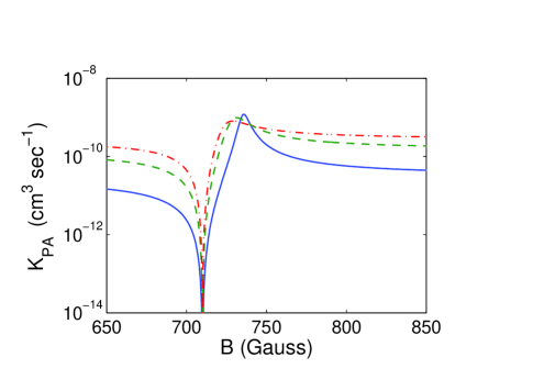
Figure 2: PA rate $K_{PA}$ in cm³ sec^-1 is plotted as a function of magnetic field $B$ in Gauss. The parameters are $\Gamma_{p}=0.1$ MHz (solid line), $\Gamma_{p}=0.5$ MHz (dashed line) and $\Gamma_{p}=1.0$ MHz (dashed-dotted line). The parameter $q_{f}$ is chosen to be - 8.90 (solid line), -7.63 (dashed) and - 6.36 (dashed-dotted) so that the minimum and maximum of $K_{PA}$ occur at $B=710$ G and $B\simeq 736$ G, respectively. The other parameters are $\gamma$ = 11.7 MHz, $S_{pc}$= - 2.8 MHz and temperature $T=10\mu$K. The laser is assumed to be tuned on resonance with the continuum-bound transition.

It is convenient to write $V_{e}=\hbar\omega_{A}+\tilde{V}_{ex}$, where $\tilde{V}_{ex}(r\rightarrow\infty)\sim-C_{3}/r^{3}$. Let $\phi_{p}$ denote the bound state solution of the the potential $\tilde{V}_{ex}$ and $E_{p}$ be the corresponding bound state (negative) energy. The Green’s function for homogeneous part with $\Lambda_{1}=\Lambda_{2}=0$ (i.e. without laser couplings) of Eq. (2) can be written as

$$G_{p}(r,r^{\prime})=-\frac{1}{\hbar\delta+E-E_{p}+i\hbar\gamma/2}\phi_{p}(r)\phi_{p}(r^{\prime})$$ (5)

where $\delta=\omega_{L}-\omega_{A}$. Using this function, we can write down the solution of equation (2) in the form $\Phi_{p}=A_{p}\phi_{p}(r)$ where

$$A_{p}=\frac{\int dr^{\prime}\left[\Lambda_{1}(r^{\prime})\chi(r^{\prime})+\Lambda_{2}(r^{\prime})\phi_{p}(r^{\prime})\right]\phi_{p}(r^{\prime})}{\hbar\delta+E-E_{p}+i\hbar\gamma/2}$$ (6)

Similarly, with the use of Green’s function for the homogeneous part of Eq. (3), we have $\Phi_{f}(r)=A_{m}\phi_{f}(r)$ where

$$A_{m} = \frac{\int dr^{\prime}\left[V^{*}(r^{\prime})\chi(r^{\prime})+A_{p}\Lambda_{2}(r^{\prime})\phi_{p}(r^{\prime})\right]\phi_{f}(r^{\prime})}{E-E_{f}}$$ (7)

where $\phi_{f}(r)$ is the wave function and $E_{f}$ is the energy of bound state in the closed channel in the absence of laser field. Now, we can express $A_{p}$ in terms of integrals involving the continuum state $\chi$ and molecular bound states $\phi_{p}$ and $\phi_{f}$. Then substituting $\Phi_{p}$ and $\Phi_{f}$ expressed in terms of $A_{p}$ and $\chi$ in Eq. (4) and making use of the relation $\chi=\int dEb_{E}\psi_{E}$, we obtain

$$-\frac{\hbar^{2}}{2\mu}\frac{d^{2}}{dr^{2}}\psi_{E}(r) + [V_{1}(r)-E]\psi_{E}(r)=-\Lambda_{1}^{*}(r)\tilde{A}_{p}\phi_{p}(r)$$ (8)

$$- \frac{(\tilde{V}_{fc}+\tilde{A}_{p}\Lambda_{pf})}{E-E_{f}}V(r)\phi_{p}(r)$$

where

$$\tilde{A}_{p}=\frac{\tilde{\Lambda}_{pc}(E-E_{f})+\Lambda_{pf}\tilde{V}_{fc}}{{\cal D}(E-E_{f})-|\Lambda_{pf}|^{2}}.$$ (9)

Here ${\cal D}=\hbar\delta+E-E_{p}+i\hbar\gamma/2$, $\tilde{V}_{fc}=\int dr\phi_{f}(r)V(r)\psi_{E}(r)$, $\tilde{\Lambda}_{pc}=\int dr\phi_{p}(r)\Lambda_{1}(r)\psi_{E}(r)$ and $\tilde{\Lambda}_{2,pf}=\int dr\phi_{p}(r)\Lambda_{2}(r)\phi_{f}(r)$. Equation (8) can now be solved by constructing the Green’s function with the scattering solutions of the homogeneous part (i.e., for $\Lambda_{1}=V=0$). This Green’s function can be written as

$${\cal K}(r,r^{\prime})=-\pi[\psi_{E}^{0,reg}(r)\psi_{E}^{0,irr}(r^{\prime})+i\psi_{E}^{0,reg}(r)\psi_{E}^{0,reg}(r^{\prime})],$$

$$\hskip 71.13188pt(r^{\prime}>r)$$

$${\cal K}(r,r^{\prime})=-\pi[\psi_{E}^{0,reg}(r^{\prime})\psi_{E}^{0,irr}(r)+i\psi_{E}^{0,reg}(r)\psi_{E}^{0,reg}(r^{\prime})],$$

$$\hskip 71.13188pt(r^{\prime}<r)$$

where the regular function $\psi_{E}^{0,reg}(r)$ vanishes at $r=0$ and the irregular solution $\psi_{E}^{0,irr}(r)$ is defined by boundary only at $r\rightarrow\infty$. These have the familiar asymptotic behavior $\psi_{E}^{0,reg}(r)\sim j_{0}\cos\eta_{0}-n_{0}\sin\eta_{0}$ and $\psi_{E}^{0,irr}(r)\sim n_{0}\cos\eta_{0}+j_{0}\sin\eta_{0}$, where $j_{0}$ and $n_{0}$ are the spherical Bessel and Neumann functions for $\ell=0$ and $\eta_{0}$ is the s-wave phase shift in the absence of laser and magnetic field couplings. Here $E=\hbar^{2}k^{2}/(2\mu)$ with $\mu$ being the reduced mass of the two atoms. Next, we can express the solution of Eq. (8) in the following form

$$\psi_{E} = \exp(i\eta_{0})\psi_{E}^{0.reg}+\int dr^{\prime}{\cal K}(r,r^{\prime})\left[\Lambda_{1}^{*}(r^{\prime})\tilde{A}_{p}\phi_{p}(r^{\prime})\right.$$ (10)

$$+ \left.\frac{\tilde{V}_{fc}^{*}+\tilde{A}_{p}\Lambda_{pf}}{E-E_{f}}V(r^{\prime})\phi_{f}(r^{\prime})\right].$$

The stimulated line width of photoassociated molecule is given by the Fermi-Golden rule expression $\Gamma_{p}=2\pi|\tilde{\Lambda}_{pc}^{0}|^{2}/\hbar$ and the Feshbach resonance line width is $\Gamma_{f}=2\pi\mid\tilde{V}_{fc}^{0}\mid^{2}/\hbar$, where $\tilde{V}_{fc}^{0}=\int dr\phi_{f}(r)V(r)\psi_{E}^{0,reg}(r)$ and $\tilde{\Lambda}_{pc}^{0}=\int dr\phi_{p}(r)\Lambda_{1}(r)\psi_{E}^{0,reg}(r)$. The Stark energy shift due to laser coupling of PM state with the continuum is given by $S_{pc}=\int\int dr^{\prime}dr\phi_{p}(r)\Lambda_{1}^{*}(r){\rm Re}[{\cal K}(r^{\prime},r)]\Lambda_{1}(r^{\prime})\phi_{p}(r^{\prime})$. Further, the physics of Feshbach resonance leads us to introduce the parameter

$$V_{pf}=\int\int dr^{\prime}dr\phi_{f}(r)V(r){\rm Re}[{\cal K}(r^{\prime},r)]\Lambda_{1}^{*}(r^{\prime})\phi_{p}(r^{\prime})$$

which represents an effective continuum-mediated magneto-optical coupling between the two bound states where $S_{fc}=\int\int dr^{\prime}dr\phi_{f}(r)V^{*}(r){\rm Re}[{\cal K}(r^{\prime},r)]V(r^{\prime})\phi_{f}(r^{\prime})$ is the energy shift of the closed channel bound state due to its coupling with the continuum. Now writing $\epsilon=(E-\tilde{E}_{f})/(\Gamma_{f}/2)$ with $\tilde{E}_{f}=E_{f}+S_{fc}$ being the shifted energy of the closed-channel bound state, and introducing a parameter

$$q_{f}=\frac{\Lambda_{pf}+V_{pf}}{\pi\tilde{\Lambda}_{pc}^{0}\tilde{V}_{fc}^{0}}$$ (11)

which we call “Feshbach asymmetry parameter”, we can express

$$\tilde{A}_{p}=\frac{\sqrt{\pi\hbar\Gamma_{p}/2}}{\hbar\Gamma_{f}/2}\left(\frac{\epsilon+q_{f}}{\epsilon+i}\right)\frac{\exp(i\eta_{0})}{\Delta_{p}+i\gamma/\Gamma_{f}+D_{I}}$$ (12)

where $\Delta_{p}=[E-(E_{p}-\hbar\delta)]/(\Gamma_{f}/2)=\epsilon-[E_{p}-\hbar\delta-\tilde{E}_{f}]/(\Gamma_{f}/2)$ is independent of laser intensity and $D_{I}=(-2S_{pc}+i\Gamma_{p})/\Gamma_{f}-(\Gamma_{p}/\Gamma_{f})(q_{f}-i)^{2}/(\epsilon+i)$ is a parameter which is proportional to laser intensity $I$. In writing the above equation we have assumed that $\tilde{V}_{fc}^{0}$, and $\tilde{\Lambda}_{pc}^{0}$ are real quantities. Note that $q_{f}$ is independent of laser power since its numerator as well as the denominator is proportional to laser amplitude. Following the Ref. verhaar , we can express $\epsilon$ in terms of applied magnetic field in the form

$$\epsilon=\frac{E-E_{th}-(E_{th}-\tilde{E}_{f})}{\Gamma_{f}/2}=\frac{E-E_{th}}{\Gamma_{f}/2}-\frac{B-B_{0}}{\Delta(ka_{bg})}$$ (13)

where $E_{th}$ is the threshold of the open channel, $\Delta$ is the Feshbach resonance width, $B_{0}$ is the resonance magnetic field and $a_{bg}$ is the background scattering length. Here $E-E_{th}$ is the asymptotic collision energy. The energy $E_{th}$ depends on the applied magnetic field due to Zeeman shift of the atomic level. The resonance scattering length is given by $a_{res}=-a_{bg}\Delta/(B-B_{0})$.

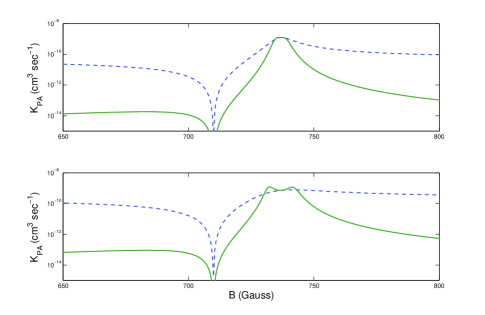
Figure 3: The dashed lines are $K_{PA}$ vs. $B$ plots when PA laser is tuned on resonance with continuum-bound transition. The solid lines are corresponding plots when the laser is tuned on resonance with bound-bound transition. For upper panel (a) $\Gamma_{p}=0.01\Gamma_{f}$, and for lower panel (b) $\Gamma_{p}=0.05\Gamma_{f}$. For both the panels, the other fixed parameters are $q_{f}=-9.0$, $\gamma=0.7\Gamma_{f}$, $T=10\mu$K, $\Gamma_{f}=16.67$ MHz and $B_{0}=736.72$ Gauss. The minimum and maximum of dashed curve in (a) appear at 710 Gauss and 736.8 Gauss, respectively.

Before we discuss our main results, we would like to point out how our mathematical treatment discussed above is related to the recent work of Koznetsova et al. Kuznetsova who have studied a related model in a different context which is to transfer of atoms into ground state molecules via two-photon process near a Feshbach resonance. Our approach is to find out the real space dressed wave function by solving time-independent scattering problem by Green’s function method while they have adapted a quantum optics-based approach of finding time-dependent amplitudes of the dressed state by solving coupled differential equations numerically.

III The results and discussion

We now discuss characteristic features of our main results. PA spectrum is given by the PA rate coefficient $K_{PA}=\langle v_{rel}\sigma_{PA}\rangle$, where $\sigma_{PA}=(\hbar\gamma|\tilde{A}_{p}|^{2})/(2\pi k^{2})$ is the cross section for the loss of atoms due to decay of the excited molecules. Here $\langle\cdots\rangle$ implies thermal averaging over the relative velocity $v_{rel}=\hbar k/\mu$. Note that, in the limit $\Gamma_{f}\rightarrow 0$, PA spectrum reduces to a Lorentzian implying that coupling between closed channel bound state and the continuum is essential for the occurrence of Fano interference. When both $\Lambda_{2}$ and $\tilde{V}_{fc}^{0}$ go to zero, the spectrum reduces to that of standard PA. For numerical illustrations, we consider a model system of two ground-state (S_1/2) ⁷Li atoms undergoing PA from the ground molecular configuration ${{}^{3}}\Sigma^{+}_{u}$ to the vibrational state $v=83$ of the excited molecular configuration ${{}^{3}}\Sigma_{g}$ which correlates asymptotically to 2S_1/2 + 2P_1/2 free atoms. The spontaneous linewidth is taken to be $\gamma=11.7$ MHz prodan . The experimental value of shift $S_{pc}$ is reported be $-1.7\pm 0.2$ MHz /W cm² prodan . The resonance width is $\Delta=-192.3$ Gauss and the background scattering length $a_{bg}=-24.5a_{0}$ ($a_{0}$ is Bohr radius) Pollack . The Feshbach resonance linewidth $\Gamma_{f}$ at 10 $\mu$K temperature is calculated out to be 16.66 MHz using the parameters reported in Ref. chin .

Depending on how PA laser is tuned, we have two cases. In the first case (case-I), laser is on or near resonance with free-bound transition but off-resonant with bound-bound transition. In the second case (case-II), it is resonant with bound-bound transition. PA rate will be maximized at the poles of Eq. (12). In case-I, there is only one pole of Eq. (12) which depends on laser intensity. The minimum in the spectrum is solely determined by the asymmetry parameter $q_{f}$ and is independent of laser intensity. We first consider case-I and plot $(K_{PA})$ as a function of $B$ for three different values of $\Gamma_{p}$ in Fig.2. For these three different $\Gamma_{p}$ values we choose three different $q_{f}$ parameters such that the maximum appears near $B=736$ G Junker:prl:2008 . Since the minimum position $B_{min}$ is independent of laser intensity, we also choose three different values of resonant magnetic field $B_{0}$ such that $B_{min}$ remains fixed at 710 G for theses three $\Gamma_{p}$ values. In this case there arises asymmetric Fano profile with one minimum and one maximum. This results from quantum interference between continuum-bound and bound-bound Raman-type transition pathways. This interpretation of Raman Fano profile is in accordance with the recent experimental observation of two-photon PA by Moal et al. moal .

Next we consider case-II in which PA laser is tuned in resonance with bound-bound rather than continuum-bound transition. In this case we have $\hbar\delta-E_{p}+\tilde{E}_{f}=0$ and so $\Delta_{p}=\epsilon$. Then $\tilde{A}_{p}$ will have two maxima given by

$$\epsilon(\epsilon+i)+i\tilde{\Gamma}_{t}(\epsilon+i)-\tilde{\Gamma}_{p}(q_{f}-i)^{2}=0.$$ (14)

where $\tilde{\Gamma}_{t}=\Gamma_{t}/\Gamma_{f}$ with $\Gamma_{t}=\Gamma_{p}+\gamma$ being the total line width, and $\tilde{\Gamma}_{p}=\Gamma_{p}/\Gamma_{f}$. For the sake of comparison, we plot spectra in Fig.3 for both the cases. Figure 3(a) shows that a single maximum appears in both the cases when laser intensities are low. As laser intensity increases, the maximum in case-I disappears while a two peak structure emerges in case-II as displayed in Fig.3(b). We notice that PA rate is lower in case-II in comparison to case-I for the same magnetic field and other parameters except near the two maxima. To further investigate into the double-peak structure, we demonstrate spectra for case-II at higher intensities in Fig.4 which clearly indicates the nonlinear features of Fano interference. The origin of the two peaks lies in Autler-Townes splitting eberly due to bound-bound resonant coupling when continuum-bound dipole coupling is scanned into two-photon resonance. At lower intensities, the two peaks can appear on the same side of Fano minimum. As a result, there can appear another smaller minimum (we call it Autler-Townes (AU) minimum in order to distinguish it from Fano minimum) between the two peaks. By comparing Fig.3(a) with Fig.3(b), we note that the AU minimum at a higher intensity appears near the position where maximum would have appeared at a lower intensity. The separation between the two maxima increases with increasing laser intensities as shown in Fig.4. As one of the peaks crosses the Fano minimum at an increased laser intensity, the AU minimum disappears due to its interference with the much stronger Fano minimum resulting in two-maximum structure only. The double-maximum structure is particularly prominent in the strong-coupling regime where $\Gamma_{p}$ exceeds the spontaneous line width $\gamma$ of PA molecule. Recently, Pellegrini and Cote pellegrini:njp:2009 have theoretically obtained double-minimum spectra using the formalism of Ref. cote2 which is to first diagonalize the part of the Hamiltonian pertaining to the ground state scattering (continuum interacting with the bound state in closed-channel), and then to calculate the optical transition matrix element between this diagonalized state and the excited molecular state by Fermi-Golden rule. This is similar to linear Fano theory Fano61 and hence can not be applied for strong-coupling that can further modify the continuum state significantly. In our formalism, we have diagonalized the full Hamiltonian nonperturbatively.

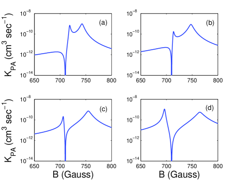
Figure 4: Shown are $K_{PA}$ vs. $B$ plots when PA laser is tuned on resonance with bound-bound transition for $\Gamma_{p}=0.5\gamma$ (a), $\Gamma_{p}=\gamma$ (b), $\Gamma_{p}=2\gamma$ (c) and $\Gamma_{p}=4\gamma$ (d). The parameters chosen are $B_{0}=730.51$Gauss, $q_{f}=-6.89$ with all others parameters remaining same as in Fig.2

IV conclusion

The results discussed above clearly demonstrate linear and nonlinear aspects of Fano interference in weak- and strong-coupling regimes, respectively. Observation of two-minimum and two-maximum structures crucially depends on precise tuning of PA laser on or near resonance with bound-bound transition. If the laser field is tuned to get the maximum amount of loss of atoms for a fixed magnetic field, the resulting PA spectrum will mostly correspond to the case-I with a single maximum. To explore the nonlinear Fano effect, it is important to know the binding energy of the closed-channel bound state so that the laser can be accurately tuned near resonance with the bound-bound transition as the magnetic field is varied. Recently, nonlinear Fano effect was observed in quantum dot Recentnaturepaper . Although Autler-Townes splitting has been recently demonstrated in two-photon PA two-photon ; moal , it is yet to be observed in PA with a single laser beam in the presence of Feshbach resonance. Fano interference may further be explored in photoassociation between heteronuclear atoms such as Na and Cs bigelow or K and Rb ni which have broad magnetic Feshbach resonance and shorter ranged excited potentials.

Acknowledgment
We are thankful to N. Bigelow for discussions. This work is supported by the NSF Grant No. PHYS 0653494.

References

- (1) U. Fano, Phys. Rev. 124, 1866 (1961).
- (2) K. Rzazewski and J. H. Eberly, Phys. Rev. Lett. 47, 408 (1981).
- (3) P. Lambropoulos and P. Zoller, Phys. Rev. A 24, 379 (1981); G. S. Agarwal et al., Phys. Rev. Lett. 48, 1164 (1982); G. S. Agarwal, S. L. Haan, and J. Cooper, Phys. Rev. A 29, 2552 (1984).
- (4) S. E. Harris , Phys. Rev. Lett. 62, 1033 (1989); S. Harris, Physics Today 50, 36 (1997); M. D. Lukin and A. Imamoglu, Nature 413, 273 (2001).
- (5) G. S. Agarwal, Quantum Statistical Theories of Spontaneous Emission and Their Relation to Other Approaches, Springer Tracts in Modern Physics: Quantum Optics (Springer-Verlag, Berlin, 1974); A. A. Svidzinsky, J. Chang, and M. O. Scully, Phys. Rev. Lett. 100, 160504 (2008).
- (6) M. O. Scully and M. S. Zubairy, Science 301, 181 (2003).
- (7) L. V. Hau et al., Nature 397, 594 (1999).
- (8) Z. Shi et al., Phys. Rev. Lett. 99, 240801 (2007).
- (9) R. Wynar et al., Science 287, 1016 (2000); K. Winkler et al., Phys. Rev. Lett. 95, 063202 (2005); C. Ryu et al., cond-mat/0508201.
- (10) R. Dumke et al., Phys. Rev. A 72, 041801(R) (2005).
- (11) S. Moal et al. Phys. Rev. Lett. 96, 023203 (2006).
- (12) J. L. Bohn and P. S. Julienne, Phys. Rev. A 60, 414 (1999).
- (13) J. L. Bohn and P. S. Julienne, Phys. Rev. A 54, R4637 (1996).
- (14) M. Junker et al., Phys. Rev. Lett. 101, 060406 (2008).
- (15) K. Winkler et al., Phys. Rev. Lett. 98,043201 (2007).
- (16) K. K. Ni et al., Science 322, 231 (2008).
- (17) M. Mackie et al., Phys. Rev. Lett. 101, 040401 (2008).
- (18) P. Pellegrini and R. Cote, New J. Phys.11, 055047 (2009).
- (19) P. Pellegrini, M. Gacesa and R. Cote, Phys. Rev. Lett. 101, 053201 (2008).
- (20) E. Kuznetsova et al., New J. Phys. 11, 055028 (2009).
- (21) E. Tiesinga, B. J. Verhaar and H. T. C. Stoof, Phys. Rev. A 47,4114 (1993); S. Inouye et al., Nature 392, 151 (1998); Ph. Courteille et al., Phys. Rev. Lett. 81, 69 (1998); J. L. Roberts et al., Phys. Rev. Lett. 81, 5109 (1998).
- (22) H. R. Thorsheim, J. Weiner, and P.S. Julienne, Phys. Rev. Lett. 58, 2420 (1987); for reviews on PA, see J. Weiner et al., Rev. Mod. Phys. 71, 1 (1999); F. Masnou-Seeuws and P. Pillet, Adv. At. Mol. Phys. 47, 53(2001); K. M. Jones et al., Rev. Mod. Phys. 78, 483 (2006).
- (23) A. J. Moerdijk, B. J. Verhaar and A. Axelsson, Phys. Rev. A 51, 4852 (1995).
- (24) I. D. Prodan et al., Phys. Rev. Lett.91 080402 (2003).
- (25) S. E. Pollack et al., Phys.Rev. Lett.102, 090402 (2009).
- (26) C. Chin et al. LANL arXiv 0812.1496 (2008).
- (27) M. Kroner et al., Nature 451, 311 (2008).
- (28) J. P. Shaffer, W. Chalupczak, and N. P. Bigelow, Phys. Rev. Lett. 82, 1124 (1999); C. Haimberger et al., Phys. Rev. A 70, 021402(R) (2004).