A general multivariate latent growth model with
applications in student careers Data warehouses

Abstract

The evaluation of the formative process in the University system has been assuming an ever increasing importance in the European countries. Within this context the analysis of student performance and capabilities plays a fundamental role. In this work we propose a multivariate latent growth model for studying the performances of a cohort of students of the University of Bologna. The model proposed is innovative since it is composed by: (1) multivariate growth models that allow to capture the different dynamics of student performance indicators over time and (2) a factor model that allows to measure the general latent student capability. The flexibility of the model proposed allows its applications in several fields such as socio-economic settings in which personal behaviours are studied by using panel data.

1 Introduction

The Bologna Process started in 1999 with the aim of creating a European Higher Education Area, in which students could choose from a wide and transparent range of high quality courses and benefit from smooth recognition procedures. The Bologna Declaration has initiated a series of reforms needed to make European Higher Education more compatible and comparable, more competitive and more attractive than before, both for Europeans and for students from other continents. Hence, the evaluation of formative processes has received a growing attention by policy makers and public agents in order to identify critical factors for achievements that can improve curricula, instructional strategies, and conditions for learning.
An important emerging problem is the comparison between students’ performances i) when different supporting and tutoring actions are adopted during the course of studies, ii) in presence of different personal situations. With this purpose, several Universities have created Data WareHouse (DWH) systems to collect detailed multivariate individual responses over time, which consist of mixtures of count, categorical, and continuous observations. These longitudinal data allow to answer questions about student progress, evaluate how each individual performs over time (within-individual change), predict the main differences among individuals in their change (interindividual differences in change). However, in presence of multidimensional observations, a challenging problem is the characterization of both temporal and cross-sectional dependencies among response variables having different measurement scales. In such cases, it is natural to consider models in which the dependency among the responses is due to the presence of both one or more latent variables and random effects, as shown in several approaches developed in the literature.
Roy and Lin (2000) proposed a 2-step linear mixed model applied to multiple continuous outcomes. These authors use time-dependent factors to account for correlations of items within time. On the other hand, a random intercept and random effects are introduced for explaining the correlations across time of both items and time-dependent latent variables, respectively. An extension to such models is provided by Dunson (2003), who introduced a dynamic latent trait model for multidimensional longitudinal data in the context of the Generalized Linear Latent Variable Model (GLLVM) so that different kinds of observed variables can be considered. An autoregressive structure that allows for covariates is used to model the structural part. The model is estimated by using the MCMC procedure. Within the same framework, a full information likelihood estimation method via the EM algorithm is developed by Cagnone et al. (2009) with particular attention to ordinal data.
A very general approach is represented by multilevel models (Skrondal and Rabe-Hesketh, 2004) that allow to deal with longitudinal and/or multidimensional mixed data. In presence of repeated measures, occasions are viewed as first level units whereas respondents are second level units. With multidimensional data, first level units are represented by items nested within individuals. When both the dimensions are considered more complex hierarchical structures have to be taken into account.
Multidimensional and longitudinal data are also treated within the traditional structural equation approach (SEM). They are modeled in two different ways.
According to the first one (Jöreskog and Sörbom, 2001), a standard confirmatory factor model is considered and its the main feature is that the corresponding error terms are correlated over time. Moreover, the latent variables are identified by setting to 1 the same loading over time.
The second approach is represented by latent growth models, widely applied in the analysis of change (Singer and Willett, 2003). Random effects are included into the model to account for the individual differences both in the initial status and in the rate of growth. The peculiar feature of such models is that the random coefficients are treated as latent variables within the traditional SEM approach (Muthén and Khoo, 1998). In this context, univariate analysis are usually performed by studying the temporal dynamics of a single indicator, considered as a proxy of the individual performance. Multivariate extensions essentially consist of modeling the trajectories of several items separately, and then to allow for correlations among random coefficients (Bollen and Curran, 2006; Raykov, 2007).
This work is motivated by the study of the data coming from the DWH of the University of Bologna. We focus on the achievements of a cohort of students enrolled in 2001 at the Faculty of Economics. Multiple items are present in the data set. Their behaviour over time can be classically analyzed by means of multivariate latent curves, where all the variability between items is captured by the correlation of the random coefficients. However, some of these items can be seen as indicators of student latent capabilities. Hence, part of their variability can be due to latent constructs. In order to take into account these two important aspects simultaneously we propose a new, general, class of models, that consists of two parts: i) multivariate latent curves that describe the behaviour of each item over time, ii) a factor model that specifies the relationship between manifest and latent variables. Although these two components have been widely developed in the literature separately, the novelty of our proposal lies in integrating them into a unique framework.

The model is developed within the GLLVM framework. According to this approach, the response variables are assumed to follow different distributions of the exponential family, with item-specific linear predictors depending on both time-specific covariates, latent variables, and measurement errors. Moreover, we extend the GLLVM by including item-specific random coefficients so that each item has its own trajectory over time. Our approach has clear advantages with respect to both multivariate latent curves since the unobservable capabilities of the single individual can be taken into account, and the dynamic factor models since we incorporate a more flexible treatment of the temporal dynamics of the items. The latter are also assumed to be heteroscedastic over time.
The paper is organized as follows. In Section 2 we present the data source and perform an exploratory analysis to demonstrate the potential of our approach in describing student performances over time. Section 3 describes the proposed methodology in terms of model specification, identification and estimation. In Section 4 we present the results of model estimation for the overall data set and for different temporal patterns observed in the sample. We conclude with a discussion in Section 5.

2 Data

The data set analyzed was extracted from the Data warehouse of the University of Bologna. This latter is a system that collects and constantly updates informations by integrating data coming from sources of different nature. The project started in 2002 in order to support planning, control and decision processes.

The DWH contains a great amount of information per each student and allows to build the overall university student career. It is also possible to find socio-demographic information (gender, country/region of origin, etc.) and the mark obtained in the final exam of the High School. We decided to analyze the cohort of $n=821$ students enrolled at the Faculty of Economics in the academic year 2001/2002 since this Faculty is one of the biggest of the University of Bologna and such year is the first available in the DWH, so that several time points can be observed.

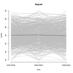
Figure 1: Trajectories of AM in the three academic years for Overall, Grad, Nograd patterns.

Therefore, this data set does not contain missing data in the first three years of the study. After the third year, the presence of missing data is due to different reasons: either students that got the degree in time (three years), or drop outs, or simply missing information. Hence, we analyzed the performance of the selected students in the first three academic years: $t_{1}=2001/2002$; $t_{2}=2002/2003$; $t_{3}=2003/2004$. In the data set, two variables are available for evaluating the student performance over time: the marks obtained in every exam and the number of exams taken per each time point. The average of the marks (AM) per each student in each academic year is considered. In the left side of Figure 1 the AM trajectories for the full sample of students are reported. They vary from 18 (minimum mark to pass the exam) to 30 (maximum mark) even if they are mostly concentrated in the range 21-28, and the overall mean (black line) is over 24 for all the observed time points. Within the selected sample we can distinguish two different temporal behaviours: the first one concerns students who got the degree in the first three years (Grad) while the second one concerns students that at $t_{3}$ did not manage to get the degree yet (Nograd). Indeed, as shown in the center and in the right side of Figure 1, the former presents a higher overall average mark and a lower variability than the latter. In Table 1 the descriptive statistics of AM for the overall sample, Grad ($n_{1}=195$) and Nograd ($n_{2}=626$) are reported. Grad presents the highest correlations over the three time points. On the other hand, Nograd is very similar to the Overall sample in terms of both first and second order moments.

Table 1: Descriptive statistics of AM in the three academic years

Overall Grad Nograd $t_{1}$ $t_{2}$ $t_{3}$ $t_{1}$ $t_{2}$ $t_{3}$ $t_{1}$ $t_{2}$ $t_{3}$ Mean $23.88$ $24.14$ $23.59$ $26.15$ $26.33$ $26.32$ $23.17$ $23.46$ $22.74$ Std Dev $4.62$ $4.10$ $5.26$ $1.85$ $1.99$ $2.05$ $4.99$ $4.34$ $5.65$ Correlations $t_{2}$ $0.41$ $0.68$ $0.34$ $t_{3}$ $0.32$ $0.37$ $0.67$ $0.76$ $0.25$ $0.29$

Table 2: Number of students per NE over time for the Overall sample, Grad and Nograd

Overall Grad Nograd NE $t_{1}$ $t_{2}$ $t_{3}$ $t_{1}$ $t_{2}$ $t_{3}$ $t_{1}$ $t_{2}$ $t_{3}$ 0 $22$ $16$ $30$ $0$ $0$ $0$ $22$ $16$ $30$ 1 $37$ $20$ $36$ $0$ $0$ $0$ $37$ $20$ $36$ 2 $59$ $60$ $53$ $1$ $1$ $0$ $58$ $59$ $53$ 3 $98$ $95$ $67$ $1$ $0$ $0$ $97$ $95$ $67$ 4 $118$ $139$ $92$ $6$ $9$ $0$ $112$ $130$ $92$ 5 $147$ $173$ $105$ $23$ $32$ $3$ $124$ $141$ $102$ 6 $167$ $149$ $161$ $61$ $63$ $53$ $106$ $86$ $108$ 7 $131$ $100$ $138$ $70$ $54$ $65$ $61$ $46$ $73$ 8 $42$ $36$ $73$ $33$ $13$ $34$ $9$ $23$ $39$ 9 - $11$ $40$ - $5$ $21$ - $6$ $19$ 10 - $8$ $21$ - $5$ $16$ - $3$ $5$ 11 - $12$ $3$ - $12$ $2$ - $0$ $1$ 12 - $2$ $0$ - $1$ $0$ - $1$ $0$ 13 - $0$ $1$ - $0$ $0$ - $0$ $1$ 14 - $0$ $1$ - $0$ $1$ - $0$ $0$

The number of exams (NE) is a count variable whose range is different in the observed time points. Table 2 shows the number of students classified according to NE both taken in the three time points and the groups defined before. The hyphens indicate that in the first academic year, a student can take at most eight exams. We can observe that, in general, Grad students present the same behaviour over the three years, that is, they take a number of exams greater than three, and concentrate it between six and seven. On the contrary, Nograd students take a number of exams equal or greater than zero, mostly concentrated between four to six. Moreover, few students of the overall sample take more than eight exams at $t_{2}$ (only $4,1\%$) and at $t_{3}$ (only $8,1\%$). It can be useful to evaluate whether i) the variable NE shows a dependence over time and ii) there is an association between the variable AM and NE within the same time. To this aim, the variable AM has been recoded for all the time points into four classes according to the quartiles of the distribution. As for the variable NE, the categories from 1 to 3 and categories from 9 to 14 have been collapsed to avoid the problem of sparseness that affects these data in the extreme categories. In Table 3 the values of the Chi square tests (with associated p-values) are reported for all the pairs of NE over time and for all the pairs of AM and NE within time. The association between AM and NE for Grad is not significant at time $t_{2}$, whereas all others are significant, indicating that both the variables can be good indicators of the student capability.

Table 3: Associations between variables

Pairs Overall Grad Nograd $\chi^{2}$ $df$ p-value $\chi^{2}$ $df$ p-value $\chi^{2}$ $df$ p-value $\text{NE}_{t_{1}}$ vs $\text{NE}_{t_{2}}$ $209.10$ $30$ $0.000$ $73.64$ $30$ $0.000$ $80.73$ $30$ $0.001$ $\text{NE}_{t_{1}}$ vs $\text{NE}_{t_{3}}$ $219.178$ $30$ $0.000$ $85.26$ $20$ $0.000$ $89.51$ $30$ $0.000$ $\text{NE}_{t_{2}}$ vs $\text{NE}_{t_{3}}$ $199.02$ $36$ $0.000$ $88.18$ $24$ $0.000$ $110.74$ $36$ $0.000$ $\text{AM}_{t_{1}}$ vs $\text{NE}_{t_{1}}$ $147.45$ $15$ $0.000$ $32.25$ $15$ $0.006$ $90.94$ $15$ $0.000$ $\text{AM}_{t_{2}}$ vs $\text{NE}_{t_{2}}$ $92.53$ $18$ $0.000$ $21.39$ $18$ $0.260$ $36.50$ $18$ $0.006$ $\text{AM}_{t_{3}}$ vs $\text{NE}_{t_{3}}$ $137.81$ $18$ $0.000$ $91.52$ $9$ $0.000$ $84.46$ $18$ $0.001$

3 Modeling and estimation

For a given student a record consists of number of exams (NE) and the average marks (AM) achieved in each academic year. Hence, in this section we present parametric growth models for mixed observations, and provide special treatment to count and continuous responses.

3.1 Multivariate latent growth curves

Suppose that $J$ items are observed for $n$ individuals at $T_{j},j=1,...,J$, different time points. The measured outcomes for a randomly selected individual are denoted by $\boldsymbol{y}=(\boldsymbol{y}_{1}^{\prime},...,\boldsymbol{y}_{j}^{\prime},...,\boldsymbol{y}_{J}^{\prime})^{\prime}$, where the elements $\boldsymbol{y}_{j}=(y_{1j},...,y_{Tj})^{\prime}$, $j=1,2,...,J$, consist of mixtures of count ($j=1,...,J_{1}$) and continuous ($j=J_{1}+1,...,J$) responses. In analyzing data of this type, a challenging problem is the characterization of both the temporal and the cross-sectional dependency among variables that have different measurement scales. In such cases, it is natural to consider models in which the dependencies are due to the presence of both several latent variables and random effects, stacked into the vector $\boldsymbol{\eta}$ (Cagnone et al., 2009). The marginal distribution of the overall responses is given by

$$f(\boldsymbol{y}|\boldsymbol{x})=\int g(\boldsymbol{y}|\boldsymbol{\eta},\boldsymbol{x})h(\boldsymbol{\eta})d\boldsymbol{\eta}$$ (1)

where $g(\boldsymbol{y}|\boldsymbol{\eta},\boldsymbol{x})$ is the conditional distribution of the responses $\boldsymbol{y}$ given a set of covariates $\boldsymbol{x}$ and the latent variables $\boldsymbol{\eta}$, and $h(\boldsymbol{\eta})$ is their prior density function. We refer to the GLLVM framework developed in Bartholomew and Knott (1999) for multivariate mixed responses and in Moustaki (2003) when covariate effects are included. We extend that framework to allow for multivariate longitudinal data. One of the main assumption of the GLLVM approach is the conditional independence of the responses (within and over time) given the latent variables, that is

$$g(\boldsymbol{y}|\boldsymbol{\eta},\boldsymbol{x})=\prod_{j=1}^{J}\prod_{t=1}^{T_{j}}g(y_{tj}|\boldsymbol{\eta},\boldsymbol{x}_{tj})$$ (2)

where $g(y_{tj}|\boldsymbol{\eta},\boldsymbol{x}_{tj})$ is a distribution of the exponential family. For count data,

$$g(y_{tj}|\boldsymbol{\eta},\boldsymbol{x}_{tj})=\left(\begin{array}[]{c}n_{t}\\ y_{tj}\\ \end{array}\right)\left(\frac{\exp(\upsilon_{tj})}{1+\exp(\upsilon_{tj})}\right)^{y_{tj}}\left(\frac{1}{1+\exp(\upsilon_{tj})}\right)^{n_{t}-y_{tj}}\qquad j=1,...,J_{1}$$ (3)

where $n_{t}$ is the number of ”trials” (or opportunities for an event). Even if counts are generally modeled using a Poisson distribution, when the events being counted for a unit occur at a constant rate in continuous time and are mutually independent, a binomial distribution is more appropriate. Indeed we will deal with counts corresponding to the number of exams that the student takes in each academic year, given the maximum number of exams $n_{t}$ observed for that year. The counts have a binomial distribution if the events for a unit are independent and equally probable. This assumption is satisfied in our model by assuming the conditional independence of the responses given the latent variables $\boldsymbol{\eta}$.
On the other hand, for continuous data

$$g(y_{tj}|\boldsymbol{\eta},\boldsymbol{x}_{tj})=\frac{1}{\sqrt{2\pi}\sigma_{tj}}\exp\left(-\frac{1}{2}\left(\frac{y_{tj}-v_{tj}}{\sigma_{tj}}\right)^{2}\right)\quad j=J_{1}+1,...,J$$ (4)

where $\sigma_{tj}^{2}$ is the variance of the continuous responses supposed to be heteroscedastic over time and between items.

As in the classical generalized linear model, $\upsilon_{tj}$ is the linear predictor for the $j$th outcome at time $t$ and the link between the linear predictor and the conditional means of the random distributions can be any monotonic differentiable function. In this context, the link is the logit of the probability associated to each count for the binomial distribution defined in eq. (3) and the identity function in the case of the normal distribution defined in eq. (4).

For both kinds of observed variables the linear predictor is defined as

$$\upsilon_{tj}=\sum_{r=0}^{p}\beta_{rj}\lambda_{t}^{r}+\sum_{k=1}^{q}\lambda_{kj}z_{k}+\sum_{l=1}^{b}\gamma_{tjl}x_{tjl}\qquad t=1,...,T_{j},\quad j=1,...,J$$ (5)

and in matrix form

$$\upsilon_{tj}=\boldsymbol{w}_{tj}\boldsymbol{\eta}+\boldsymbol{\gamma}_{tj}\boldsymbol{x}_{tj},\qquad j=1,...,J$$ (6)

where

$$\boldsymbol{w}_{t1} = [1,\lambda_{t},...,\lambda_{t}^{p},...,0,...,0,\lambda_{11},\lambda_{21},...,\lambda_{q1}],$$

$$\cdots \cdots\qquad\cdots$$

$$\boldsymbol{w}_{tJ} = [0,...,0,...,1,\lambda_{t},...,\lambda_{t}^{p},\lambda_{1J},\lambda_{2J},...,\lambda_{qJ}],$$

$$\boldsymbol{\gamma}_{tj} = [\gamma_{tj1},...,\gamma_{tjb}],$$

$$\boldsymbol{x}_{tj} = [x_{tj1},...,x_{tjb}].$$

The latent variables $\boldsymbol{\eta}=(\beta_{0j},...,\beta_{pj},z_{1},...,z_{q})$ are random effects and latent traits that account for both the temporal and the cross-sectional dependence between items. The $\gamma_{tjl}$ are fixed regression parameters representing the effects of the covariates $x_{tjl},l=1,...,b$. As it is done with ”classical” univariate growth models, the random coefficients $\boldsymbol{\beta}_{j}=(\beta_{0j},...,\ldots,\beta_{pj})$, $j=1,...,J$, and the corresponding loadings $\lambda_{t},t=1,...,T_{j}$, are introduced in order to describe the temporal behaviour of each item, $p$ being the degree of the fitted trajectory. The $\lambda_{t}$’s either can be fixed, in the case of linear polynomials, or can be parameters to be estimated if a nonlinear function is more appropriate. The model is very flexible since it allows to specify different temporal dynamics for each item. The common factors $\boldsymbol{z}=(z_{1},\ldots,z_{q})$ can represent traits of an individual (e.g. general and specific student abilities, intelligence, etc. ) and determines the correlation between multiple responses despite their temporal behaviour.

By defining the linear predictor in this way, the temporal dependence between items as well as the autocorrelation of each item are explained by variance and covariance elements related to the random growth parameters $\boldsymbol{\beta}_{j},j=1,...,J$. On the other hand, the cross-correlation between items despite their temporal behaviour is caught by the factor model via the loadings $\boldsymbol{\lambda}_{jz}=(\lambda_{j1},...,\lambda_{jq}),j=1,...,J$. These assumptions are contained in the prior density function of the latent variables, $h(\boldsymbol{\eta})$, supposed to be a multivariate normal density with mean vector $\boldsymbol{\mu}_{\boldsymbol{\eta}}=(\mu_{\beta_{01}},...,\mu_{\beta_{p1}},...,\mu_{\beta_{0J}},...,\mu_{\beta_{pJ}},0,...,0)$ and covariance matrix $\boldsymbol{\Psi}=\left(\begin{array}[]{cc}\boldsymbol{\Psi}_{\beta}&\mathbf{0}\\ \mathbf{0}&\boldsymbol{\Psi}_{z}\\ \end{array}\right),$ where $\boldsymbol{\Psi}_{\beta}$ is the full covariance submatrix related to the random effects $\boldsymbol{\beta}_{j},j=1,..,J$, and $\boldsymbol{\Psi}_{z}$ is the submatrix of the block matrix related to the latent factors $\boldsymbol{z}$. We assume that the random coefficients $\boldsymbol{\beta}_{j}$ and the factors $\boldsymbol{z}$ are independent. Furthermore, some constraints must be placed to ensure identifiability of the model based on the observed data. In particular, as in classical latent variable models, there is indeterminacy related to the scales of the latent factors $\boldsymbol{z}$ (Jöreskog, 1969). This indeterminacy can be eliminated by either setting $\lambda_{1j}=1$ or letting the variances of the factors be one, with at least one of the loadings constrained to be positive for each factor.

As a consequence of the structural specification of the model via $h(\boldsymbol{\eta})$, the covariances between different responses, seeing in the scale provided by the link function, are given by

$$\text{Cov}(v_{tji},v_{t^{\prime}ji}) = \boldsymbol{w}_{tj\beta}\Psi_{\beta}\boldsymbol{w}_{t^{\prime}j\beta}^{\prime}+\boldsymbol{w}_{jz}\Psi_{\beta}\boldsymbol{w}_{jz}^{\prime}$$

$$\text{Cov}(v_{tji},v_{tj^{\prime}i}) = \boldsymbol{w}_{tj\beta}\Psi_{\beta}\boldsymbol{w}_{tj^{\prime}\beta}^{\prime}+\boldsymbol{w}_{jz}\Psi_{\beta}\boldsymbol{w}_{j^{\prime}z}^{\prime}$$

$$\text{Cov}(v_{tji},v_{t^{\prime}j^{\prime}i}) = \boldsymbol{w}_{tj\beta}\Psi_{\beta}\boldsymbol{w}_{t^{\prime}ji\beta}^{\prime}+\boldsymbol{w}_{jz}\Psi_{\beta}\boldsymbol{w}_{j^{\prime}z}^{\prime}$$

where $\boldsymbol{w}_{tj\beta}$ and $\boldsymbol{w}_{jz},t=1,2,...,T_{j},j=1,2,...,J$, indicate the coefficients in $\boldsymbol{w}_{tj}$ related to the random effects $\boldsymbol{\beta}_{j},j=1,...,J,$ and the latent traits $\boldsymbol{z}$, respectively.

3.2 Estimation

The parameters of the model are estimated through the Maximum Likelihood (ML) method via the EM algorithm, since the latent variables $\boldsymbol{\eta}$ are unobserved. The EM starts with initial values of the parameters. The algorithm consists of an expectation and a maximization step. In the expectation step the expected score function from the complete likelihood ($\boldsymbol{y},\boldsymbol{\eta}|\boldsymbol{x}$) given the covariates is computed. In the maximization step updated parameter estimates are obtained from the equations derived in the E-step. The whole procedure is repeated until convergence.

For a random sample of size $n$, it follows by eq. (1) that the complete log-likelihood is written as:

$$L = \sum_{i=1}^{n}\log f(\boldsymbol{y}_{i},\boldsymbol{\eta}_{i}|\boldsymbol{x}_{i})$$ (7)

$$= \sum_{i=1}^{n}\left[\log g(\boldsymbol{y}_{i}|\boldsymbol{\eta}_{i},\boldsymbol{x}_{i})+\log h(\boldsymbol{\eta}_{i})\right]$$

where $g$ is the likelihood of the data conditional on the covariates, the latent variables and the random effects and $h$ is the common distribution function of the latent traits and the random effects. From eq. (7), we see that the first component depends on both the factor loadings $\boldsymbol{\lambda}_{jz},j=1,...,J$ and the variance parameters $\boldsymbol{\sigma}_{j}^{2}=(\sigma_{1}^{2},...,\sigma_{T_{j}}^{2}),j=J_{1}+1,...,J,$ whereas the second component depends on $(\boldsymbol{\mu}_{\boldsymbol{\eta}},\boldsymbol{\Psi})$.

3.2.1 Estimation of $\boldsymbol{\mu}_{\boldsymbol{\eta}}$ and $\boldsymbol{\Psi}$

From the normality of $\boldsymbol{\eta}$, the second component of the log-likelihood given in eq. (7) (up to a constant) for an individual $i$ is written as

$$\log h(\boldsymbol{\eta}_{i})=-\frac{1}{2}\ln\boldsymbol{\Psi}-\frac{1}{2}(\boldsymbol{\eta}_{i}-\boldsymbol{\mu}_{\boldsymbol{\eta}})\boldsymbol{\Psi}^{-1}(\boldsymbol{\eta}_{i}-\boldsymbol{\mu}_{\boldsymbol{\eta}})^{\prime}.$$ (8)

The expected score function needed for the EM implementation is taken with respect to the posterior distribution of the latent variables $h(\boldsymbol{\eta}_{i}|\boldsymbol{y}_{i},\boldsymbol{x}_{i})$. The expected score function for the parameter vector $\boldsymbol{\mu}_{\eta}$ becomes

$$ES_{i}(\boldsymbol{\mu}_{\eta})=\int S_{i}(\boldsymbol{\mu}_{\eta})h(\boldsymbol{\eta}_{i}|\boldsymbol{y}_{i},\boldsymbol{x}_{i})d\boldsymbol{\eta}_{i},\qquad i=1,...,n$$ (9)

where

$$S_{i}(\boldsymbol{\mu}_{\eta})=\frac{\partial\log h(\boldsymbol{\eta}_{i})}{\partial\boldsymbol{\mu}_{\eta}}=\boldsymbol{\Psi}^{-1}(\boldsymbol{\eta}_{i}-\boldsymbol{\mu}_{\boldsymbol{\eta}}).$$

Similarly, we obtain the score function for $\boldsymbol{\Psi}$, that is,

$$S_{i}(\boldsymbol{\Psi})=\frac{\partial\log h(\boldsymbol{\eta}_{i})}{\partial\boldsymbol{\Psi}}=-\frac{1}{2}\boldsymbol{\Psi}^{-1}-\frac{1}{2}\boldsymbol{\Psi}^{-1}(\boldsymbol{\eta}_{i}-\boldsymbol{\mu}_{\boldsymbol{\eta}})(\boldsymbol{\eta}_{i}-\boldsymbol{\mu}_{\boldsymbol{\eta}})^{\prime}\boldsymbol{\Psi}^{-1}.$$

By solving $\sum_{i=1}^{n}ES_{i}(\boldsymbol{\mu}_{\eta})=0$ and $\sum_{i=1}^{n}ES_{i}(\boldsymbol{\Psi})=0$ we get explicit solutions for the maximum likelihood estimators of $\boldsymbol{\mu}_{\eta}$ and $\boldsymbol{\Psi}$.

3.2.2 Estimation of $\boldsymbol{\lambda}_{jz}$ and $\boldsymbol{\sigma}_{j}^{2}$

The estimation of parameters $\boldsymbol{\lambda}_{jz},j=1,...,J$ and $\boldsymbol{\sigma}_{j}^{2},j=J_{1}+1,...,J$ depends on the first component of the log-likelihood given in eq. (7). Under the conditional independence assumption, the log-likelihood of the count and continuous data can be written as

$$\log g(\boldsymbol{y}_{i}|\boldsymbol{\eta}_{i},\boldsymbol{x}_{i}) = \sum_{j=1}^{J_{1}}\sum_{t=1}^{T_{j}}\left[\log\left(\begin{array}[]{c}n_{t}\\ y_{tji}\\ \end{array}\right)+y_{tji}\upsilon_{tji}-n_{t}\log\left(1+\exp(\upsilon_{tji})\right)\right]+$$ (12)

$$+ \sum_{j=J_{1}+1}^{J}\sum_{t=1}^{T_{j}}\left[-\frac{1}{2}\log(2\pi)-\frac{1}{2}\log(\sigma_{tj}^{2})-\frac{(y_{tji}-\upsilon_{tji})^{2}}{2\sigma_{tj}^{2}}\right]$$ (13)

The first component refers to count variables and will be used to derive estimates of the factor loadings corresponding to such variables, that is, $\boldsymbol{\lambda}_{jz},j=1,...,J_{1}$. The expected score function of the parameter vector $\lambda_{jz}$ is again taken with respect to the posterior $h(\boldsymbol{\eta}_{i}|\boldsymbol{y}_{i},\boldsymbol{x}_{i})$:

$$ES_{i}(\boldsymbol{\lambda}_{jz})=\int S_{i}(\boldsymbol{\lambda}_{jz})h(\boldsymbol{\eta}_{i}|\boldsymbol{y}_{i},\boldsymbol{x}_{i})d\boldsymbol{\eta}_{i},\quad i=1,...,n$$ (14)

where

$$S_{i}(\boldsymbol{\lambda}_{jz})=\frac{\partial\log g(y_{tji}|\boldsymbol{\eta}_{i},\boldsymbol{x}_{i})}{\partial\boldsymbol{\lambda}_{jz}},$$

and

$$\frac{\partial\log g(y_{tji}|\boldsymbol{\eta}_{i},\boldsymbol{x}_{i})}{\partial\boldsymbol{\lambda}_{jz}}=\sum_{t=1}^{T_{j}}\boldsymbol{z}_{i}\left(y_{tji}-n_{t}\frac{\exp(\upsilon_{tji})}{(1+\exp(\upsilon_{tji}))}\right)\qquad j=1,...,J_{1}.$$ (15)

By replacing eq. (15) into eq. (14) and solving $\sum_{i=1}^{n}ES_{i}(\boldsymbol{\lambda}_{jz})=0$ we get non-explicit solutions for the parameter vector $\boldsymbol{\lambda}_{jz}$. A Newton-Raphson algorithm is used to solve the nonlinear maximum likelihood equations.

From the second component in the likelihood (13) we estimate factor loadings and variance components corresponding to continuous items. The expected score functions for the parameters $\boldsymbol{\lambda}_{jz},j=J_{1}+1,...,J$, are given by

$$ES_{i}(\boldsymbol{\lambda}_{jz})=\int S_{i}(\boldsymbol{\lambda}_{jz})h(\boldsymbol{\eta}_{i}|\boldsymbol{y}_{i},\boldsymbol{x}_{i})d\boldsymbol{\eta}_{i},\qquad i=1,...,n$$ (16)

where

$$S_{i}(\boldsymbol{\lambda}_{jz})=\sum_{t=1}^{T_{j}}\boldsymbol{z}_{i}^{2}\lambda_{jzi}-\sum_{t=1}^{T}\boldsymbol{z}_{i}(y_{tji}-\sum_{r=0}^{p}\beta_{rj}\lambda_{t}^{r}).$$

Similarly, we obtain the score function for each element in $\boldsymbol{\sigma}_{j}^{2},j=J_{1}+1,...,J$, that is,

$$S_{i}(\sigma_{tj}^{2})=\sigma_{tj}^{2}-(y_{tji}-\upsilon_{tji})^{2}\qquad t=1,...,T_{j},\quad i=1,...,n.$$

By solving $\sum_{i=1}^{n}ES_{i}(\boldsymbol{\lambda}_{jz})=0,\sum_{i=1}^{n}ES_{i}(\boldsymbol{\sigma}_{j}^{2})=0$ we get explicit solutions for the maximum likelihood estimators of $\boldsymbol{\lambda}_{jz}$ and $\boldsymbol{\sigma}_{j}^{2}$ for $j=J_{1}+1,...,J$.

Integrals are approximated by using Gauss-Hermite quadrature points. In order to apply the Gauss-Hermite approximation to the integral of equations (9), (14), and (16) we consider the Cholesky decomposition of the covariance matrix $\boldsymbol{\Psi}$ given by $\boldsymbol{\Psi}=\boldsymbol{C}\boldsymbol{C}^{\prime}$. As shown by Cagnone et al. (2009), this is necessary because the non null submatrices of $\boldsymbol{\Psi}$, namely $\boldsymbol{\Psi}_{\boldsymbol{\beta}}$ and $\boldsymbol{\Psi}_{\boldsymbol{z}}$, are not diagonal.

The steps of the EM algorithm are defined as follows:

Step 1:

choose initial estimates for the model parameters. Starting values for the loadings are obtained by fitting separate confirmatory factor analysis models at each time points. Initial values for the other parameters are chosen arbitrarily.

Step 2:

compute the expected score functions for all the parameters (E-step).

Step 3:

obtain improved estimates for the parameters by solving the nonlinear maximum likelihood equations for the parameters corresponding to the count items and explicit solutions for the parameters of the continuous items and the latent distribution (M step).

Step 4:

repeat steps 2-3 until convergence is attained.

4 Results

We start the analysis by estimating a model for the overall dataset of students observed at the three different time points. As already discussed, the aim of the analysis is twofold: (1) analyze the student careers over time with respect to the Number of Exams taken in each occasion (NE) and the corresponding Average Marks (AM), and (2) measure the general latent capability of the students. Therefore, we analyze how the variables NE and AM change over time by means of multivariate latent growth models, and we extend these models by including a common factor that can explain the atemporal variability that exists between the two items. In particular, since only three different academic years are considered, a linear polynomial model ($p=1$) could be appropriate to describe the temporal pattern of both NE and AM. Measurement invariance over time of the loadings in the one-factor model ($q=1$) is assumed. Thus, the estimated model (denoted as Model A) is characterized by the following linear predictor

$$\upsilon_{tj}=\beta_{0j}+\beta_{1j}(t-1)+\lambda_{j}z=\boldsymbol{w}_{tj}\boldsymbol{\eta},\qquad t=1,2,3,\quad j=NE,AM$$

where

$$\boldsymbol{w}_{tNE} = [1,0,1,2,0,0,0,0,\lambda_{NE}]$$

$$\boldsymbol{w}_{tAM} = [0,0,0,0,1,0,1,2,\lambda_{AM}],$$

$$\boldsymbol{\eta} = [\beta_{0NE},\beta_{1NE},\beta_{0AM},\beta_{1AM},z].$$

Binomial-logistic and Normal heteroscedastic linear regression models are estimated for the NE and AM, respectively. The multivariate normal density of the latent variables $h(\boldsymbol{\eta}$) has mean vector $\boldsymbol{\mu}_{\boldsymbol{\eta}}=(\mu_{\beta_{0NE}},\mu_{\beta_{1NE}},\mu_{\beta_{0AM}},\mu_{\beta_{1AM}},0)$ and covariance matrix $\boldsymbol{\Psi}=\left(\begin{array}[]{cc}\boldsymbol{\Psi}_{\beta}&\mathbf{0}\\ \mathbf{0}&1\\ \end{array}\right).$ For identification reasons, the variance of the common latent factor $z$ is set equal to 1.
FORTRAN and R codes have been implemented to estimate the model. (They are available from the authors upon request). Parameter estimates of Model A for the overall dataset are reported in Table 4.

Table 4: Estimates for the overall data set (standard errors in brackets)

Model A Coefficients Estimates Multivariate growth model $\hat{\mu}_{\beta_{0}NE}$ $\hskip 7.11317pt0.249$ $(0.047)$ $\hat{\mu}_{\beta_{1}NE}$ $-0.443$ $(0.026)$ $\hat{\mu}_{\beta_{0}AM}$ $\hskip 7.11317pt23.98$ $(0.326)$ $\hat{\mu}_{\beta_{1}AM}$ $-0.113$ $(0.244)$ $\hat{\boldsymbol{\Psi}}_{\beta}$ $\left(\begin{array}[]{cccc}$\hskip 2.84544pt0.231$^{*}&&&\\ $-0.107$^{*}&$\hskip 2.84544pt0.093$^{*}&&\\ $\hskip 2.84544pt1.004$^{*}&$-0.531$^{*}&$\hskip 1.42271pt 4.980$^{*}&\\ $-0.363$^{*}&$\hskip 1.42271pt 0.413$^{*}&$-2.183$^{*}&$2.164$^{*}\\ \end{array}\right)$ *: significant at $5\%$ level. Factor model $\hat{\lambda}_{NE}$ $\hskip 4.26773pt0.524$ $(0.073)$ $\hat{\lambda}_{AM}$ $\hskip 4.26773pt2.581$ $(0.449)$ $\hat{\sigma}_{1AM}^{2}$ $10.080$ $(0.340)$ $\hat{\sigma}_{2AM}^{2}$ $\hskip 4.26773pt9.953$ $(0.176)$ $\hat{\sigma}_{3AM}^{2}$ $14.568$ $(0.395)$

It can be noticed that both NE and AM present similar temporal dynamics, even if expressed on different scales. In terms of the population mean trajectory, NE presents a mean initial status equal to 0.249, indicating that in the first year the students take, in mean, around 4.5 exams, as expressed in the original scale. The students’ progress is described by the slope mean parameter $\mu_{\beta 1}$, equal to -0.443, reflecting the linear, term-by-term, worsening in mean achievement during the second and third years. Both the mean initial status and rate of growth are coherent with the descriptive analyses we performed in Section 2, since on average the number of exams, as derived by Table 2, were 4.76, 4.43, and 4.47 in $t_{1},t_{2},t_{3}$, respectively. Similarly, at the initial status, students obtain an average mark (in mean) around 23.98, but this mean worsens over time as indicated by the mean slope parameter $\hat{\mu}_{\beta_{1}AM}$ equal to $-0.133$.
By looking at the covariances specific of each item in $\hat{\boldsymbol{\Psi}}_{\beta}$, students present a higher variability in the initial status than in the rate of growth, with a negative correlation between initial status and slope, for both NE and AM. Multivariate latent curves also allow to analyze the covariation between the temporal dynamics of NE and AM by estimating cross-covariances between random intercepts and slopes of the two curves. There are positive and significant covariances between $\beta_{0NE}$ and $\beta_{0AM}$ as well as between the random slopes, $\beta_{1NE}$ and $\beta_{1AM}$, indicating that students with higher (smaller) average marks in the first year tend to take a higher (smaller) number of exams at $t_{1}$, and that students with positive (negative) slopes for AM generally present a similar pattern for NE. On the other hand, negative covariances are estimated between $\beta_{0NE}$ and $\beta_{1AM}$ as well as between $\beta_{0AM}$ and $\beta_{1NE}$. Differently from classical multivariate latent growth modeling, these cross-covariances between NE and AM curves are free from the effect of a common latent factor $z$ we estimated via integrating the growth curves with a one factor model.

When manifest variables are of different types, care is needed in the interpretation of the factor loadings, depending on the scale of the $y_{tj}$. In order to interpret the latent factor $z$ we shall therefore have to ensure that the $\lambda$s are calibrated so that they may be meaningfully compared across variable types. This may be done in a variety of ways but we follow the approach of Takane and De Leeuw (1987) and Bartholomew and Knott (1999), which provides a parametrization that keeps the interpretation as close as possible to the familiar methods of traditional factor analysis. This approach is based on a standardization of the coefficients of the latent variable $z$ in order to express correlation coefficients between the manifest variable $y_{tj}$ and the factor $z$.
For the normal item, $\lambda_{AM}$ denotes the covariance between the manifest variables $y_{tAM}$ and the factor $z$. By dividing $\lambda_{AM}$ by the square root of the variance of the continuous variable $y_{tAM},t=1,2,3$, we obtain the correlation between $y_{tAM}$ and $z$, that is

$$\lambda_{tAM}^{*}=\frac{\lambda_{AM}}{\sqrt{\psi_{\beta_{0AM}}^{2}+2(t-1)\psi_{\beta_{0AM},\beta_{1AM}}+(t-1)^{2}\psi_{\beta_{1AM}}^{2}+\lambda_{AM}^{2}+\sigma_{tAM}^{2}}},\qquad t=1,2,3.$$ (17)

Notice that the correlation varies over time, hence

$$\hat{\lambda}_{1AM}^{*} = 0.554$$

$$\hat{\lambda}_{2AM}^{*} = 0.586$$

$$\hat{\lambda}_{3AM}^{*} = 0.505$$

The amplitude of the factor loadings is quite similar in all the three occasions and on average is equal to $0.548$, indicating that the measurement invariance assumption is appropriate.
On the other hand, for the binomial item, the standardization follows that proposed for binary items (Moustaki and Knott, 2001) and based on the equivalence of the response function and underlying variable approaches (Takane and De Leeuw, 1987). In this context, the correlation between a normal variable supposed to be underlying the binomial discrete observations and the latent variable $z$ is given by

$$\lambda_{tNE}^{*}=\frac{\lambda_{NE}}{\sqrt{\psi_{\beta_{0NE}}^{2}+2(t-1)\psi_{\beta_{0NE},\beta_{1NE}}+(t-1)^{2}\psi_{\beta_{1NE}}^{2}+\lambda_{NE}^{2}+1}},\qquad t=1,2,3.$$ (18)

The estimated standardized binomial loadings are

$$\hat{\lambda}_{1NE}^{*} = 0.427$$

$$\hat{\lambda}_{2NE}^{*} = 0.445$$

$$\hat{\lambda}_{3NE}^{*} = 0.435$$

which are really close to each other; the amplitude of the standardized factor loadings is on average $0.436$. The standardized coefficients given for normal and binomial variables can be used for a unified interpretation of the loadings, bringing the interpretation close to factor analysis. The common factor $z$ explains the interrelationships between the two observed items net from their temporal dependence. Both variables are significant indicators of this latent capability. Moreover, they both influence positively this unobserved construct. Ignoring the presence of a common factor in multivariate latent growth models can lead to an overestimation of the cross-variation among multiple curves.

The goodness of fit of Model A has been checked separately for the count and continuous part (Moustaki and Knott, 2001). As for the count part of the model, significant information concerning the goodness of fit can be found in the margins. In particular, the one-way margins of the differences between the observed ($O$) and expected ($E$) frequencies under the model are investigated; any large discrepancies will suggest that the model does not fit well these counts. The Chi square test as well as high-way margins are not appropriate because of the sparseness of the data (Reiser, 1996). Table 5 gives the GF-fit measures, calculated as $((O-E)^{2}/E)$, for each Binomial variable (Bartholomew et al., 2002).

Table 5: Count items: GF-fit values for the one-way margins.

Counts $y_{1EN}$ $y_{2EN}$ $y_{3EN}$ 0 11.58 11.65 11.23 1 0.10 1.59 3.05 2 5.78 0.22 10.39 3 5.45 0.39 15.20 4 8.73 4.97 5.91 5 1.10 16.18 0.95 6 7.58 5.12 34.35 7 24.47 0.33 37.70 8 3.65 23.75 2.33 9 - 31.37 0.04 10 - 13.06 0.66 11 - 0.31 7.94 12 - 0.02 0 13 - - 0.41 14 - - 1.23

We can observe that the GF-fits are not good, especially those on count 7 for $y_{1NE}$, on 8 and 9 for $y_{2NE}$, and on counts 6 and 7 for $y_{3NE}$. Reasons of this misfitting of Model A on the overall sample will be next investigated.

For the normal part of the model we check the discrepancies between the sample correlation matrix and the one estimated from the model, as illustrated in Table 6 for the variables $y_{1AM},y_{2AM}$, and $y_{3AM}$.

Table 6: Normal items: discrepancies between sample and estimated correlation matrices.

$y_{1EN}$ $y_{2EN}$ $y_{3EN}$ $y_{1EN}$ 0.00 -0.05 0.02 $y_{2EN}$ -0.05 0.00 -0.05 $y_{3EN}$ 0.02 -0.05 0.00

The discrepancies between observed correlations and those estimated are particularly small, indicating that the fit of the model for the normal variables is good.

In Section 2, we showed that among the 821 students, two different temporal patterns were evident, one related to those students who graduated at $t_{3}$ (Grad) and the other to students who did not get the degree regularly at the third year (Nograd). Hence, we shall analyze these two different groups of students in order to investigate the reasons of the poorness of fit for the count part of the Model A in the overall dataset. Therefore, in the following, we fit Model A to the Grad and Nograd students, separately.

4.1 The Graduate students

We first consider the $195$ students who graduated at $t_{3}$, and we start by fitting the Model A described above. The results of the estimation are reported in Table 7. It can be noticed that parameter estimates corresponding to both the multivariate latent growth and the factor parts of Model A differ substantially from what we obtained for the overall sample. As for the former, both NE and AM present higher mean initial status than the overall sample. They are equal to $6.05$ for NE and to $26.17$ for AM, as expressed in the original scales. Furthermore, the mean trajectory for NE has a worsening pattern over time, whereas the one corresponding to AM presents an increasing but not significant temporal behaviour. By looking at the variability around the mean trajectories, this is significant in the initial status ($0.133$) and in the rate of growth ($0.072$) corresponding to NE which also shows a negative correlation between the random intercept and slope. On the other hand, there is not a significant variability for AM with respect to its mean trajectory, indicating that the Grad students show a similar pattern over time. This finding is also evident in all the (not significant) covariances between random coefficients of NE and AM.

As for the factor part, the loading associated to the binomial variable is very close to 0 and not significant, suggesting that the number of exams for these students is not a measure of their capability. However, also the loading associated to AM is not significant. This means that for Grad students it makes no sense to specify a common factor related to the variables AM and NE. A justification could be found from the not significant association between AM and NE for Grad in time $t_{2}$, as shown in Section 2. This evidence can be a hint to test the assumption of measurement invariance over time. If we estimate a model where this assumption is relaxed, denote it as Model B (Table 7), we can notice that the time dependent loadings are very different. This is particularly true for the variable NE, for which the loading does not change greatly in the first two time points but becomes negative in $t_{3}$. For the variable AM the loading increases over time. Clearly, the measurement invariance cannot be assumed. This result is also confirmed by the AIC and BIC criteria that show that Model B is better than Model A. However, from our viewpoint, Model B is meaningless in the factor part. Moreover, if we look at the one-way margins associated to Model B (Table 8) we can see that again there are goodness of fit problems at time points $t_{2}$ and $t_{3}$.
These results for Grad highlight two different aspects of the analysis. First of all, we have a slight individual variability around NE and AM mean trajectories, indicating a similar temporal behaviour of these students. Moreover, the higher values of these means compared to those obtained for the overall sample show a good performance of this group. Secondly, in this case the two variables are not measures of a latent construct that in the overall sample we identified as capability.

Table 7: Estimates for graduate (Grad) students

Model A Coefficients Estimates Multivariate growth model $\hat{\mu}_{\beta_{0}NE}^{2}$ $1.133$ $(0.086)$ $\hat{\mu}_{\beta_{1}NE}^{2}$ $-0.577$ $(0.050)$ $\hat{\mu}_{\beta_{0}AM}^{2}$ $26.172$ $(0.149)$ $\hat{\mu}_{\beta_{1}AM}^{2}$ $0.080$ $(0.061)$ $\boldsymbol{\Psi}_{\beta}$ $\left(\begin{array}[]{cccc}$0.133$^{*}&&&\\ $-0.097$^{*}&$0.072$^{*}&&\\ $0.441$&$-0.327$&$2.197$&\\ $0.044$&$-0.026$&$-0.086$&$0.376$\\ \end{array}\right)$ *: significant at $5\%$ level. Factor model $\hat{\lambda}_{NE}$ $0.005$ $(0.262)$ $\hat{\lambda}_{AM}$ $0.670$ $(3.360)$ $\hat{\sigma}_{1AM}^{2}$ $0.702$ $(0.147)$ $\hat{\sigma}_{2AM}^{2}$ $1.292$ $(0.113)$ $\hat{\sigma}_{3AM}^{2}$ $0.328$ $(0.185)$ AIC= 4304.090 BIC= 4309.602 Model B Coefficients Estimates Multivariate growth model $\hat{\mu}_{\beta_{0}NE}^{2}$ $1.193$ $(0.093)$ $\hat{\mu}_{\beta_{1}NE}^{2}$ $-0.594$ $(0.066)$ $\hat{\mu}_{\beta_{0}AM}^{2}$ $26.225$ $(0.192)$ $\hat{\mu}_{\beta_{1}AM}^{2}$ $0.188$ $(0.079)$ $\boldsymbol{\Psi}_{\beta}$ $\left(\begin{array}[]{cccc}$0.136$^{*}&&&\\ $-0.103$^{*}&$0.078$^{*}&&\\ $0.445$&$-0.340$&$2.727$&\\ $0.025$&$-0.021$&$-0.167$&$0.317$\\ \end{array}\right)$ *: significant at $5\%$ level. Factor model $\hat{\lambda}_{1NE}$ $0.300$ $(0.413)$ $\hat{\lambda}_{2NE}$ $0.465$ $(0.594)$ $\hat{\lambda}_{3NE}$ $-0.103$ $(0.185)$ $\hat{\lambda}_{1AM}$ $0.156$ $(0.339)$ $\hat{\lambda}_{2AM}$ $0.440$ $(0.571)$ $\hat{\lambda}_{3AM}$ $0.734$ $(0.886)$ $\hat{\sigma}_{1AM}^{2}$ $0.616$ $(0.129)$ $\hat{\sigma}_{2AM}^{2}$ $1.300$ $(0.114)$ $\hat{\sigma}_{3AM}^{2}$ $0.351$ $(0.177)$ AIC= 4226.847 BIC= 4273.520

Table 8: Count items: GF-fit values for the one-way margins, Model B.

Counts $y_{1EN}$ $y_{2EN}$ $y_{3EN}$ 2 0.34 0.05 - 3 4.65 - - 4 7.46 0.03 - 5 4.20 16.28 18.16 6 1.37 58.32 11.10 7 5.29 13.48 19.52 8 0.86 15.12 0.00 9 - 23.81 0.40 10 - 14.41 0.50 11 - 0.02 2.35 12 - 1.38- - 13 - - - 14 - - 30.51

4.2 The Nograduate students

Coherently with the previous analysis, we first estimated Model A for Nograd students. The results are reported in Table 9. The growth model shows results similar to the overall sample with a higher variability for AM with respect to its mean trajectory.

Table 9: Estimates for Undergraduate (Nograd) students

Model A Coefficients Estimates Multivariate growth model $\hat{\mu}_{\beta_{0}NE}^{2}$ $-0.030$ $(0.055)$ $\hat{\mu}_{\beta_{1}NE}^{2}$ $-0.353$ $(0.035)$ $\hat{\mu}_{\beta_{0}AM}^{2}$ $23.337$ $(0.431)$ $\hat{\mu}_{\beta_{1}AM}^{2}$ $-0.183$ $(0.326)$ $\boldsymbol{\Psi}_{\beta}$ $\left(\begin{array}[]{cccc}$\hskip 0.56917pt 0.171$^{*}&&&\\ $-0.109$^{*}&$\hskip 0.56917pt 0.131$^{*}&&\\ $\hskip 0.56917pt 0.930$^{*}&$-0.610$^{*}&$ 5.514$^{*}&\\ $-0.552$^{*}&$\hskip 0.56917pt 0.658$^{*}&$-3.304$^{*}&$3.492$^{*}\\ \end{array}\right)$ *: significant at $5\%$ level. Factor model $\hat{\lambda}_{NE}$ $0.473$ $(0.119)$ $\hat{\lambda}_{AM}$ $2.609$ $(0.706)$ $\hat{\sigma}_{1AM}^{2}$ $12.356$ $(0.567)$ $\hat{\sigma}_{2AM}^{2}$ $12.484$ $(0.269)$ $\hat{\sigma}_{3AM}^{2}$ $17.307$ $(0.612)$ AIC= 18773.348 BIC= 18788.483 Model C Coefficients Estimates Multivariate growth model $\hat{\mu}_{\beta_{0}NE}^{2}$ $-0.031$ $(0.051)$ $\hat{\mu}_{\beta_{1}NE}^{2}$ $-0.353$ $(0.032)$ $\hat{\mu}_{\beta_{0}AM}^{2}$ $23.346$ $(0.406)$ $\hat{\mu}_{\beta_{1}AM}^{2}$ $-0.215$ $(0.294)$ $\boldsymbol{\Psi}_{\beta}$ $\left(\begin{array}[]{cccc}$\hskip 0.56917pt 0.184$^{*}&&&\\ $-0.117$^{*}&$\hskip 0.56917pt 0.133$^{*}&&\\ $\hskip 0.56917pt 0.935$^{*}&$-0.619$^{*}&$5.180$^{*}&\\ $-0.570$^{*}&$\hskip 0.56917pt 0.709$^{*}&$-3.241$^{*}&$4.052$^{*}\\ \end{array}\right)$ *: significant at $5\%$ level. Factor model $\hat{\lambda}_{NE}$ $0.464$ $(0.079)$ $\hat{\lambda}_{AM}$ $2.502$ $(0.620)$ $\hat{\sigma}_{AM}^{2}$ $13.642$ $(0.234)$ AIC= 18777.719 BIC= 18791.260

Table 10: Count items: GF-fit values for the one-way margins, Model A, Nograd.

Counts $y_{1EN}$ $y_{2EN}$ $y_{3EN}$ 0 7.69 11.56 5.01 1 0.86 1.67 4.91 2 7.91 0.18 9.11 3 3.48 1.33 8.28 4 2.16 7.46 0.17 5 1.01 12.83 2.96 6 9.86 0.33 20.67 7 12.61 7.89 8.47 8 0.27 10.92 0.41 9 - 14.13 0.27 10 - 5.54 3.57 11 - - 3.21 12 - 0.35 - 13 - - 1.53

In this case the results related to the factor model are very interesting. Differently from what we found for the Grad group, the loadings are both significant and positively related to the latent variable and indicate that, as in the overall data set, the factor model is appropriate. Differently from what we found in all previous analysis, the GF-fits of this model are satisfactory for all the observed time points, as reported in Table 10. Thus the count part of the model is well fitted by the binomial distribution. Also for the normal part the fit is very good, the discrepancies between observed and estimated correlations being very low (Table 11). Therefore, Model A fits well the Nograd students data.

Table 11: Normal items: discrepancies between sample and estimated correlation matrices, Model A, Nograd.

$y_{1EN}$ $y_{2EN}$ $y_{3EN}$ $y_{1EN}$ 0.00 -0.07 0.02 $y_{2EN}$ -0.07 0.00 -0.08 $y_{3EN}$ 0.02 -0.08 0.00

If we look again at Table 9 Model A, it can be noticed that the values of $\sigma^{2}_{AM}$ are quite similar over time; thus, it can be interesting to evaluate if AM is homoscedastic over time. The results of the estimation of the model with homoscedastic errors (Model C) are reported in the bottom part of Table 9. Although all the parameter estimates do not change abruptly, the AIC and BIC are slightly better for Model A than for Model C, suggesting that such assumption does not hold. Thus, the comparison between the loadings of AM and NE for evaluating the influence of each item on the latent variable requires their standardization according to eq. (17) for AM and to eq. (18) for NE. We get the following standardized loadings: $\hat{\boldsymbol{\lambda}}_{AM}^{*}=(0.525,0.560,0.534)$, and $\hat{\boldsymbol{\lambda}}_{NE}^{*}=(0.401,0.414,0.388)$. As in the overall data set, the correlation between $z$ and AM is slightly higher than that between $z$ and NE.

5 Discussion

In this paper we extended and applied multivariate latent growth models to the analysis of student record data collected repeatedly in the Data warehouse system of the University of Bologna. The proposed approach is innovative since it allows to evaluate both the student performance over time and individual capabilities simultaneously. Key features include i) a flexible modeling of the temporal dynamics of the observed variables via specific latent curves, and ii) an extension of the multivariate growth model that incorporates a factor part. Such component explains the association between the observed items by means of latent variables, interpreted as different traits or capabilities.
The complexity of the model proposed lies in different aspects, such as the presence of mixed data, the possibility of both including several latent variables/random effects and estimating specific temporal patterns for the observed variables. Hence, computational problems occur in the parameter estimation. We successfully solved them by implementing an ad hoc EM algorithm (Fortran and R code are available upon request by the authors). As far as we know, commercial software does not allow to treat all these aspects simultaneously.

We demonstrated, via different specifications of the model, how our general approach can provide insights into the data structure. In particular, the analysis carried out on a cohort of students enrolled at the Faculty of Economics observed at three different time points highlighted an heterogeneity in the overall data set in terms of both average marks and number of exams. This is due to the presence of different temporal patterns within the cohort, since we have students who regularly graduate at $t_{3}$ (Grad) and students who did not manage to get the degree within the third year (Nograd). Grad students perform very well in terms of both number of exams and average marks with similar temporal pattern. Nograd take a lower number of exams with lower average marks, but within this group we have a significant variability both in the initial status and in the rate of growth. The factor part of the model for the Grad student fails in measuring a general capability by means of the observed indicators considered. We found that this fact depends on the fundamental assumption of measurement invariance of items over time. Such assumption does not hold in this case. On the contrary, the model fits well the data of Nograd students. What we called atemporal latent capability is well measured by the average mark and the number of exams taken, both being significantly related to the latent variable. The good performance of the model is confirmed by the analysis of some goodness of fit statistics.
The heterogeneity observed in the patterns of graduate and nograduate students has implications on the results of the overall data set. On the one hand parameter estimates for the overall sample are quite similar to those of Nograd students, the factor loadings of the two variables being both significant. This is in part due to the larger sample size of Nograd students. However, the presence of different performances of the Grad students reflects on the poorness of fit of the count variable in the overall data set.

The model proposed here was motivated by the study of the students’ achievements and the good results obtained clearly show its appropriateness. However, such methodology can be applied successfully in many other fields, such as socio-economic settings in which personal behaviours are studied by using panel data collected through the administration of questionnaires.

In the present example no covariates have been considered. In practice, we may have useful time dependent and time independent covariates such as gender, region of origin, age, etc. that can be incorporated into the model. In particular, an emerging field of investigation is based on the comparison of the performances of students who completed the degree compared with those who abandoned (Smith and Naylor, 2001; Draper and Gittoes, 2004). Furthermore, the treatment of missing data would allow to extend our analysis to more time points and evaluate if non linear or higher degree polynomial trajectories can describe the temporal behaviour of the items studied. Preliminary studies performed with the software LISREL (Bianconcini et. al, 2007) showed how different latent curves can fit the weighted average marks for different groups of students within the cohort analyzed. Such problems will motivate our future investigations along these lines of research.

References

- (1)
- Bartholomew and Knott (1999) Bartholomew D.J. and Knott M. (1999). Latent Variable Models and Factor Analysis. London: Hodder Arnold.
- Bartholomew et al. (2002) Bartholomew D.J, Steele F., Moustaki I., Galbraith J. (2002). Analysis and Interpretation of Multivariate Data for Social Scientists. Chapman and Hall/CRC
- Bianconcini et. al (2007) Bianconcini S., Cagnone S., Mignani, S. and Monari, P. (2002). A latent curve analysis of unobserved heterogeneity in University student achievements Statistica. 1, pp. 40-56
- Bollen and Curran (2006) Bollen K.A and Curran P.J. (2006). Latent Curve Models: a Structural Equation Perspective. New York:John Wiley and Sons.
- Cagnone et al. (2009) Cagnone S., Moustaki I. and Vasdekis V. (2009). Latent variable models for multivariate longitudinal ordinal responses. British Journal of Mathematical and Statistical Psychology. in press.
- Draper and Gittoes (2004) Draper D. and Gittoes M. (2004). Statistical analysis of performance indicators in UK higher education Journal of the Royal Statistical Society: Series A (Statistics in Society). 167,3, pp. 449-474.
- Dunson (2003) Dunson D.B. (2003). Dynamic Latent Trait Models for Multidimensional Longitudinal Data. Journal of American Statistical Association. 98, 463, pp. 555-563.
- Jöreskog (1969) Joreskog K. (1969). A General Approach to Confirmatory Maximum Likelihood Factor Analysis. Psychometrika. 34, 183-202.
- Jöreskog and Moustaki (2001) Jöreskog K. amd Moustaki I. (1969). Factor analysis of ordinal variables: A comparison of three approaches. Multivariate Behavioral Research. 36, 347-287.
- Jöreskog and Sörbom (2001) Jöreskog K. and Sörbom D. (2001). LISREL 8: Users Reference Guide. SSI, Chicago, Second Edition.
- Moustaki (2003) Moustaki I. (2003) A generalized class of latent variable models for ordinal manifest variables with covariate effects on the manifest and latent variables. British journal of mathematical and statistical psychology. 53, 337-357.
- Moustaki and Knott (2001) Moustaki I. and Knott M. (2001) Generalized latent trait models. Psychometrika. 65, 391-411.
- Muthén and Khoo (1998) Muthén B. and Khoo S.T. (1998) Longitudinal studies of achievement growth using latent variable modeling. Learning and Individual Differences. 10, 73-101.
- Reiser (1996) Analysis of residual for the multinomial item response model. Psychometrika. 61, 509-528.
- Raykov (2007) Raykov T. (2007). Longitudinal Analysis With Regressions Among Random Effects: A Latent Variable Modeling Approach. Structural Equation Modeling: A Multidisciplinary Journal. 14, 1, pp. 146 169.
- Roy and Lin (2000) Roy, J. and Lin, X. (2000). Latent Variable Models for Longitudinal Data with Multiple Continuous Outcomes. Biometrics. 56, 4, pp. 1047 - 1054.
- Singer and Willett (2003) Singer J.D. and Willett J.B. (2003). Applied Longitudinal Data Analysis: Modeling Change and Event Occurrence. New York: Oxford University Press.
- Skrondal and Rabe-Hesketh (2004) Skrondal, A. and Rabe-Hesketh S. (2004). Generalized Latent Variable Modeling: Multilevel, Longitudinal, and Structural Equation Models. Boca Raton, FL: Chapman and Hall/CRC.
- Smith and Naylor (2001) Smith J.P. and Naylor R.A. (2001). Dropping out of university: A statistical analysis of the probability of withdrawal for UK university students Journal of the Royal Statistical Society: Series A (Statistics in Society). 164,2, pp. 389-405.
- Takane and De Leeuw (1987) Takane Y. and De Leeuw J. (1987). On the relationship between item response theory and factor analysis of discretized vaiables Psychometrika. 52, pp. 393-408.