The Fate of the Initial State Perturbations in Heavy Ion Collisions
Abstract
Heavy ion collisions at RHIC are well described by the (nearly ideal) hydrodynamics. In the present paper we study propagation of perturbations induced by moving charges (jets) on top of the expanding fireball, using hydrodynamics and (dual) magnetohydrodynamics. Two experimentally observed structures, called a “cone” and a “hard ridge”, have been discovered in dihadron correlation function with large- trigger, while “soft ridge” is a similar structure seen without hard trigger. All three can be viewed as traces left by a moving charge in matter, on top of overall expansion. A puzzle is why those perturbations are apparently rather well preserved at the time of the fireball freezeout. We study two possible solutions to it: (i) a “wave-splitting” acoustic option and (ii) a “metastable electric flux tubes”. In the first case we show that rapidly variable speed of sound under certain conditions leads to secondary sound waves, which are at freezeout time closer to the original location and have larger intensities than the first wave. In the latter case we rely on (dual) magnetohydrodynamics, which also predicts two cones or cylinders of the waves. We also briefly discuss metastable electric flux tubes in the near- phase and their relation to clustering data.
I Introduction
The issues to be discussed are somewhat similar in nature to what happened in cosmology in the last decades. While the average Hubble-like expansion of the Universe has been dramatically confirmed by the discovery of background radiation more than 40 years ago, more recent observations of small-amplitude temperature fluctuations have transformed cosmology into a much more quantitative science.
Similarly, experimental data obtained in heavy ion collisions at RHIC were shown to be in very good agreement with hydrodynamical description of the “Little Bang”. Especially good results are obtained in hydrodynamics supplemented by the hadronic cascades hydro ; Hirano:2004ta ; Nonaka:2006yn . Dissipative effects from viscosity provide only small corrections, at the few percent level, see more in Romatschke:2007mq ; Dusling:2007gi ; Heinz:2008qm . Except for rather short time of initial accelration, the hydro solution can actually be rather well approximated by Hubble flow with being approximately space and time-independent . If so, the expansion can be approximated by a quite simple form
| (1) |
which we will use below.
In the last few years RHIC experiments have focused more on two and three-particle correlations, which revealed rather rich phenomenology
of correlations. These correlations appear due to certain fluctuations, propagating on top of the overall Hubble-like expantion.
Quite puzzling dynamics of such perturbations is the subject of this paper.
We will turn to experimental observations in the next section: but before we do so, let me formulate the main
dilemma of this work:
either
(A) these perturbations are
in nature, although propagating a bit differently
from what can be naively expected on the basis of a geometric optics,
or (B)
they are not hydrodynamical but include certain extra fields/structures, affecting
their expansion.
In this work we will examine whether both of those solutions are viable. The option (A) – to be referred to as the “acoustic solution” – will reveal creation of the secondary waves, induced by time-dependent speed of sound. (In fact this effect was already noticed in Ref. CasalderreySolana:2005rf in connection with conical flow.) As we will show, such secondary waves are brighter and smaller in size, as sketched in Fig.3(c). However, as we will find, it is not clear whether solution A will be viable quantitatively, as it require rather sharp drop in a speed of sound.
The second option B also leads to double cones, now as two components of Alfven waves in a (dually)magnetized medium. Furthermore, some of them have small or even zero expansion velocity, and indication to existence of stabilized electric flux tubes in near-Tc temperature interval. Metastable microscopic flux tubes in the near- region had also been considered in a different context before, by Liao and myself Liao:2007mj ; Liao:2008vj in connection with lattice data on lattice potentials and charmonium survival. Yet again, although such tubes have good reasons to exist, the final conclusion on whether they are robust enough to explain the observed “cone” and two “ridges” would require a lot of further experimental and theoretical work.
Early stages of heavy ion collisions are believed to be described by the so called “glasma” , a set of random color fields created by color charges of partons of the two colliding nuclei at the moment of the collision McLerran:1993ni . For large nuclei those charges and fields can become large enough to be treated classically. However as two discs with charges move away from each other, those classical field are getting smaller and (in a still poorly understood process) rather quickly create the quark-gluon plasma, in which the occupation numbers becoming .
Perturbative theory of asymptotically hot QGP predicts perturbative electric screening mass from the one-loop perturbative polarization tensor Shuryak:1977ut . However perturbative approach provides no screening of the static magnetic fields, , like in the QED plasma. The crucial difference between the QED and QCD plasmas lies in the existence of magnetically charged quasiparticles – monopoles and dyons – leading to nonzero magnetic screening mass first suggested by Polyakov 30 years ago Polyakov:1978vu and by now well confirmed by subsequent lattice studies. Thus hot QGP, unlike the electromagnetic plasmas, screen the electric and the magnetic fields at some microscopic scales, although at a bit different ones.
Furthermore, recent theory developments known as “magnetic scenario” Liao_ES_mono ; Chernodub:2006gu for the near- region show that the situation with electric and magnetic screening masses get in fact inverted in this region. Multiple lattice studies, e.g. ref Nakamura:2003pu have shown that at the relation between electric and magnetic screening masses get inverted, . As the electric screening mass strongly decreases, partly because of heavy quark and gluon quasiparticles and partly because of their suppression by small Polyakov loop expectation value , going to zero below . As temperature decreasing toward the magnetic screening mass is instead increasing monotonously, to a rather large value
| (2) |
Such behavior of screening as well as other theoretical considerations had lead to the “magnetic scenario” Liao_ES_mono ; Chernodub:2006gu , which basically views the near- region ( up to 1.4) as magnetic-dominated plasma, dominated by (gluomagnetic) monopoles/dyons. (It was formally known as the “M-phase”, from “mixed” of the 1st order transition, can now also be called M-phase from “magnetic”. ) Furthermore, even “electric-dominated” QGP, at , has viscosity and diffusion strongly influenced by electric-magnetic scattering Liao_ES_mono ; Ratti:2008jz .These effects provide a natural explanation for unusually small viscosity observed at RHIC and also predicting its value at the LHC.
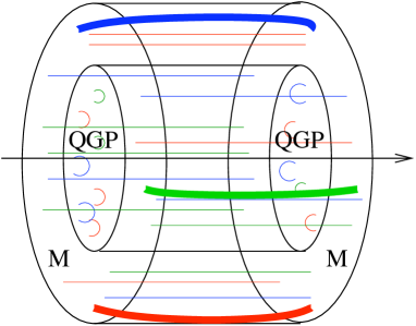
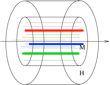
The most important consequence of that for the present paper is that in the M-phase of the collision the magnetic field is well screened while the one remains (nearly) . This leads to the central new idea of this paper: that QGP produced in central part of RHIC collisions should have a “dual corona” in which (rather than magnetic) fields coexist with the plasma, affecting both the overall expansion and the propagation of perturbations. We will suggest to use “dual magnetohydrodynamics” (DMHD) for the description of diffuse electric fields in the M-phase, in particular study their effect on the velocity of propagation of small perturbations. We will further argue below that like solar corona, that of QGP should have metastable flux tubes, although microscopically thin ones which cannot be directly described by DMHD approximation.
The word “corona” used here comes from the physics of the Sun. Let me briefly remind the reader that it was started by Galileo Galilei, who in 1612 spent some time observing the motion of the black spots on the Sun and correctly concluded from motion of the spots that they must resign on a surface of a rotating sphere: he thus argued the spots were not shadows of some planets passing in front, as it was thought of before. In due time relation between the spots and solar magnetism was understood: modern telescopes allows one to see the fine structure of solar spots, resolving individual magnetic flux tubes. Better understanding of solar magnetism came with the advance of plasma physics in 1940’s and development of MHD, which explained both the influence of diffuse magnetic field on plasma and formation and mechanical stability of the flux tubes. The MHD flux tubes are supported by the electron current, while the positive charges – the ions – are heavy and dont move. Since it is not a supercurrent, there is inevitable friction and thus metastability of the flux tube solutions.
As at RHIC the central part of the produced fireball reaches relatively high temperature , we expect both fields to be effectively screened there, see the central cylindrical part of Fig.1 marked QGP. But in the near- region vanishing electric component leads to vanishing electric screening mass. This means that plasma in the outer cylindrical part of Fig.1 marked M (mixed or magnetic) is nearly pure magnetic. It is very important to emphasize that although this region on the phase diagram is represented by a very narrow strip , it corresponds to more than order of variation of the energy or entropy density, and the corresponding space-time volume in the expansion of the fireball is by no means small. I A snapshot of the geometry of the M region at some early time is shown in Fig.1: here are unscreened electric fields (thin lines) and magnetic flux tubes (think lines). The lower plot show similar snapshot at collision energy much smaller than at RHIC, planned to be investigated in a specialized run.
II New structures observed in two and three particle correlations
II.1 The cone and the ridges
Three different correlation phenomena have been discovered in
heavy ion collisions at RHIC:
(i) the so called “cone” STAR_cone ; PHENIX_cone , is a two-peaked structure
seen in azimuthal distribution of hadrons on the “away-side” from a trigger hadron
(the region off quenched companion jet);
(ii) the so called “hard ridge” seen on the “same-side”
in the triggered events
Putschke ;
(iii) and the “soft ridge” observed in 2-particle correlations
without any hard trigger Adams:2005aw in the minijet region,
with transverse momenta .
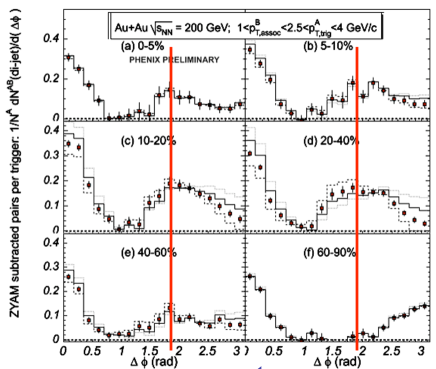
(i) The “cone” has been discovered in the 2-particle azimuthal correlations like the one shown in Fig.2. One can see from this figure the disappearance of the “away-side” peak at and appearance of new peaks at completely different angle, as one moves from peripheral to central collisions. After discovery of those effects there was extensive studies of the 3-particle correlations as well. This is a rather complicated subject to go into here, let me just say that they has confirmed the observed structure is indeed cone-like, and not e.g. a reflected jet.
(ii) the hard ridge is also seen in 2-particle correlators, but plotted on the two-dimensional plane, the differences between the azimuthal angles and pseudorapidities of the two particles. The jet remnants make a peak near , which was found to sit on top of the “ridge”, with comparable width in but very wide width . For plots and various features one can consult the original talk by Putschke Putschke . Later it was shown by PHOBOS collaboration phobos that the rapidity range of the ridge extends at least up to .
(iii) the “soft ridge” is found by STAR collaboration Adams:2005aw ; star_ridge without a trigger, in the 2-particle correlations.
For many experimental details and phenomenological considerations related to these phenomena the reader may consult e.g. the talks at recent specialized workshop cathie_workshop .
We will return to these observations below,
turning now to
their suggested explanations:
(i) Stoecker et al,
as well as Casalderrey, Teaney and myself conical have proposed
that the energy deposited by a quenched jet goes into two
hydrodynamical excitation modes, the sound and the so called diffusion or wake modes.
The sound from the propagating jet should thus create the famous Mach cone,
in qualitative agreement with the conical structure observed.
(ii) One early model for “hard ridge” has been
introduced in my paper Shuryak:2007fu . It relates it with the
forward-backward jets accompanying any hard scattering, providing
extra particles (“hot spot”) widely distributed in rapidity.
This idea is then combined with the one suggested previously by
Voloshin Voloshin:2003ud , namely that extra particles
deposited in the fireball would be moved transversely by the radial
hydrodynamical flow, should produce a peak at certain
azimuthal angle corresponding to the position of the hot spot, see Fig.3(a).
While particles of the ridge are separated by large rapidity gaps and cannot
communicate during the expansion process,
their azimuthal emission angles remain correlated with each other because they originate from
the same “hot spot” in the transverse plane.
(iii) Similarly, transverse hydro boost of “hot spots” was used for the
explanation of the “soft ridge”
by McLerran and collaborators
Dumitru:2008wn ; Gavin:2008ev . They have pointed out that
the initial state color fluctuations in the
colliding nuclei would create longitudinal “color flux tubes”
any hard collisions.
As these tubes are being stretched between two fragmentation regions
of the colliding nuclei, they also lead to long-range rapidity
correlations.

II.2 Naive hydrodynamics and the remaining puzzles
So, at a very qualitative level the origin of all three phenomena seem to be explained: yet at more qualitative level a lot of puzzles appear. As an example, consider the simplest of them, the “soft ridge”. As discussed in Dumitru:2008wn ; Gavin:2008ev , the initial stage (proper time where is the so called saturation scale at RHIC) can be discussed using classical Yang-Mills equations: thus color fluctuations naturally appear. However, the observed pions come from final freezeout time, separated from the initial “glasma” era by much longer time . This is certainly so, as the explanation heavily relies on radial hydro velocity and thus it has to wait till the hydro velocity is being created. As we will argue below, there are many reasons why one might have expected nearly complete disappearance of this signal during this time.
Common to all three cases is deposition of some additional energy (or entropy), on top of the “ambient matter”. The number of correlated particles in all of them constitute a small fraction of the total multiplicity: thus they can only be seen in a high-statistics correlation analysis. Furthermore, simple estimates show that it would not be possible to detect any trace of that tiny perturbation if it would be distributed over a significant fraction of the fireball: the only possibility is that it remains well localized in transverse direction.
Smallness of perturbation in respect to total system size by itself does not guarantee that the perturbations is small , in respect to local density of ambient matter. However it will become so if perturbation would give rise to divergent conical (or cylindrical, or spherical) waves, see Fig.3(b). Similar to circles from a stone thrown into a pond, initial perturbation may become some waves, with basically nothing left at the original location at later time. Even without dissipation, ideal hydrodynamics predicts that the final radius of those waves is given by the “sound horizon”
| (3) |
As we will detail below, by the the freezeout proper time , this distance is not small, or so, since the speed of sound changes between in QGP and about at its minimum near The amplitude of the wave is decreasing accordingly, and the width of distribution grows, making us wandering if any trace of the perturbation can remain observable.
And yet, we observe all three correlations, as if nothing happened to them during rather long time of the hydro process, . This is the puzzle discussion/resolution of which is the main objective of this paper. The idea behind it is that there can be some reasons providing second unusual mode of propagation, with reduction or maybe even vanishing of the speed of its spread and lead to an observable structures at late time, see see Fig.3(c).
(In the case of a cone, additional consideration is that the “wake” mode, behind the jet, is – in contrast – not expanding or weakening: and yet it is observed. In the case of ridges, large size of waves comparable to nuclear radius will make the radial flow directions be rather different at different places, widening the peak in azimuth well beyond what is actually observed. The puzzle is especially clear in the case of “ridges”, whose explanation heavily rely on substantial hydrodynamical flow velocity, which cannot be formed promptly and is known to be developed only by the freezeout time.)
Let me now add few more important observations on the soft ridges. The spectra of particles in cone and ridges, as well as their composition (not shown) are drastically different from jet remnants Putschke . Particularly telling is large baryon/meson ratio which clearly indicate that their existence is related to the ambient matter boosted by the hydrodynamical flow. The boosted baryons and sharpening of the peak nicely confirm that the particles of the ridge do come late, from the final freezeout of the system.
The fact that the cones and ridges are best seen for secondaries with is also a confirmation of their hydro origin. The famous elliptic flow also is maximal at such momenta, as is the baryon/meson ratio following from the radial flow. Hydro effects in general are increasing with and thus are maximal at the upper limit of hydro description, which is exactly in this region, as viscosity corrections tell us.
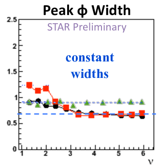
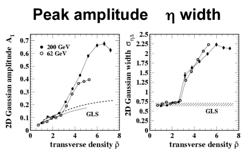
Further confirmation of hydro origin of ridges comes from the centrality dependence of the angular width of the ridge: the peak in azimuth for more central collisions, see Fig.4. This happens because of two interrelated effects, both well documented. For central collisions there is (i) an of the radial hydro velocity, accompanied by (ii) a substantial in the freezeout temperature (which goes from in peripheral down to for central collisions.
Now, let us return to the puzzles.The observed width of the azimuthal peaks provides strong limits on how large is the “spot” at the freezeout moment. In Fig.5 we have plotted the shape of azimuthal peak produced by (semi) circles of radii 1..6 fm. To see those, one has to do a very simple calculation, superimposed the radial Hubble flow with the circular spot, and calculated this angular distribution. As one can see from this figure, the width of the distribution grows – it is 0.57, 0.56, 0.69, 0.76, 0.83, 0.89 for the 6 curves shown. Moreover, the distribution shapes become very different from that observed, with two maxima shifted from (corresponding to direction of flow at two points at which the circle intersect the fireball boundary). Comparing such distribution with observations, e.g. their width with those shown in Fig.4,one finds that the radius of a spot at freezeout is restricted to be or so. As we already argued in the Introduction, this is already by about factor two smaller than the radius of the “sound horizon” expected with the realistic speed of sound . Therefore, naive picture of expanding hydro waves is in direct contradiction to data.
Having mentioned the main puzzle, let me also point out other cases of qualitative differences between the overall hydro expansion and the (soft) ridge. The latter has dramatic centrality dependence shown in Fig.6, sharply disappearing at cenrtain centrality. (The lines and shaded area marks GLS is some simple scaling expected from noninteracting minijet event generator: it only describe the data at peripheral bins at small densities). Furthermore, the comparison of the 200 and 62 GeV AuAu data shows that the transition point seem to be at the transverse particle density , so one may naively think that for the matter is simply too dilute to show hydrodynamical effects. Yet in fact both radial and elliptic flows have quite smooth centrality dependence and show no rapid changes at the same point at all.
This difference between ridges and overall hydro flows may be directly related to the main dilemma of this paper. If the cones and ridges are hydrodynamical, then why can they be so different from overall hydrodynamical expansion in their centrality dependence?
Strong temperature dependence can in principle be related to the issue of timing of the energy deposition. There is a difference between timing of the “cone” and “ridges”: while the latter obviously originate early, for “cones” the exact energy deposition time/place depends on the jet quenching mechanism. As gluon (or light quark) jets move with a speed of light, by the time of the order of nuclear size they either leave the fireball, or are already completely quenched. Recently purely geometrical study of angular distribution of quenching Liao:2008dk indicated that most of jet quenching rate should happen in the near- region. It is surprising, taking into account much higher density of QGP at earlier time.
Another dramatic finding, pointing to the same direction, was unexpected observation of similar “cones” by CERES and NA49 collaborations at much lower collision energy of CERN SPS (see recent summary by Appelhauser in cathie_workshop ). Since at the SPS energy there is practically no QGP phase, it can only be there starting in the near- (mixed) phase.
Obviously we would like to see what happens with the ridges at lower collision energies. Note that both explanations we propose in this work have problems with QGP away from : it is hard to stabilize the flux tube there and also impossible to stop expansion of the sound waves with rather large sound speed . And yet ridges disappear in very peripheral collisions: we would like to know what happens as the collision energy gets lower. (Those questions are presumably be addressed by the expected scan down in RHIC energy, planned in the nearest future.)
Another surprising experimental fact is quite large value of the cone angle, deduced from 2 and 3-particle correlators. It seems to be in the range radians (not too far from or cylindrical waves!). The Mach formula gives the speed of pertinent perturbation to be about
| (4) |
well below the expected speed of sound (except maybe near ). So again, it is either (A) a coil effect, reducing expansion, or (B) a sound with a nontrivial production mechanism.
III Acoustical waves in expanding fireball with variable speed of sound
III.1 Model equation of motion
Now we turn to discussion of the evolution of small perturbations sitting on top of overall (Hubble-like) expansion. Equations for this case have been worked out by Casalderrey-Solana and myself in Ref. CasalderreySolana:2005rf , and applied to “conical flow” conical from quenched jets. In this paper we have already found that in the vicinity of the QCD phase transition there is a wave splitting phenomenon. The framework we will use to study the effects of the variable speed of sound and matter expansion we have looked for the simplest example possible, keeping the problem time-dependent but homogeneous in space. This can be achieved in a Big-Bang-like setting in which the space is created dynamically by gravity. Consider a liquid in flat Freedman-Robertson-Walker metric :
| (5) |
where the parameter (the instantaneous Hubble radius of our “universe”) is treated as external (not to be derived from Einstein equations but from hydrodynamical solution. For isotropic expansion only the longitudinal projection is needed, which is the equation of entropy conservation leading to
| (6) |
for any R(t), provided expansion is adiabatic.
A simple substitution of a variable into the equations of motion for perturbations is inconsistent. One should instead find a correct non static solution of the hydrodynamical equations and only then, using this solution as zeroth order, study first order perturbations such as sound propagation. The linearized equations for hydrodynamical perturbations in this background has been derived in CasalderreySolana:2005rf . Using the normalized perturbation
| (7) |
one may eliminate other components of the stress tensor and get the following single equation
| (8) | |||
In the derivation we have not assumed any particular expansion function or particular equation of state, just general thermodynamic relations.
In Ref. CasalderreySolana:2005rf we have used a bit different time variable and Fourier decomposition in space, reducing the problem to an oscillator with the time-dependent frequency and specific exciting force (the third term) which is for . Note that it creates amplification of dimensionless perturbation, which is similar to the case of Universe expansion effect on small perturbations, running away from each other.
III.2 Generation of the secondary wave
Let us remind the setting in which the solutions were studied. We have already explained that we expect the expansion to be exponential and the value was fixed from matter expansion. For simplicity, we use the same expansion in 3d, although in heavy ion collisions the longitudinal expansion is different.
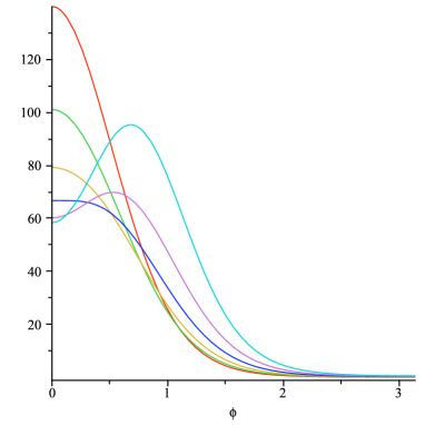
The main ingredient is the variable speed of sound . As we have already emphasized in the Introduction, at early stages at RHIC the matter is believed to be in the form of quark-gluon plasma (QGP), and thus with . This makes the third term in our eqn (8): which is nice since in this stage the Hubble flow is not yet a good approximation. In the near- region the energy density is increasing much more rapidly than the pressure, which makes matter “soft” and dropping to its minimum, known as the “softest point”. Aftre that is rising again, in the hadronic “resonance gas”. Our model-dependent time histories at two transverse position are depicted in Fig.8, for three different scenarios we would study.
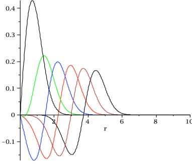
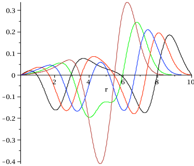
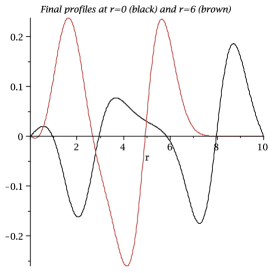
Solutions for eqn (8) corresponding to Fig.8(a) (the sharpest change) for initial Gaussian perturbation is shown in the Fig.7. In each cases we show in three pictures subsequent stages of evolution for as profiles taken every fm/c. We start with 5 curves of the fireball history, Figs.7(a) corresponding to the QGP era. Since the main new (third) term in (8) is absent, and our solution corresponds to “naive evolution” of the original perturbation into expanding primary wave. No visible trace of the perturbation remains at the initial position, and their are no secondary waves.
In Figs.7(b) we show what happens during the mixed phase: the evolution of perturbations slows down as expected. One also finds growth in amplitude, and also the secondary wave starts to appear. Figs.7(c) show that in the hadronic phase both waves start propagating outward – if there is time left to freezeout.
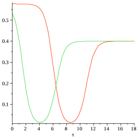
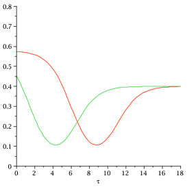
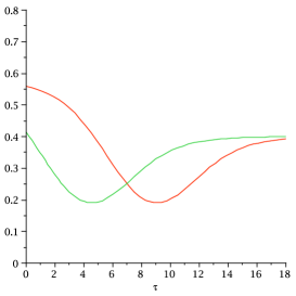
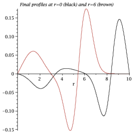
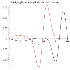
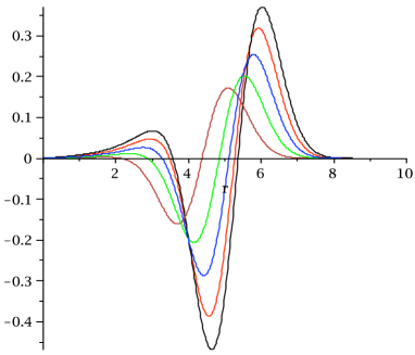
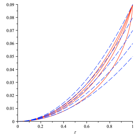
We have further studied how the amplitude of the secondary wave depends on the variation of speed of sound. For this purpose we have used e.g. 3 scenarios depicted in Fig. 8. In Fig.9 (a-c) we show the final profile of the wave at freezeout, for two histories corresponding to (the fireball center) and (fireball rim).
Let us start with (a) in which one finds of the secondary wave at the rim of about the same magnitude as the primary wave. It means that the sound intensity (which scales as ) is for the secondary wave about an order of magnitude larger. This would make the secondary wave much more likely candidate to be observable.
Furthermore, the azimuthal angular width of the ridge observed experimentally is less than 1 rad, see Fig4. Given the magnitude of the rapidity of the radial flow – up to 0.7 near the edge of the firebal and known thermal spread of secondaries at freezeout, one can explain the observed width the spot size remains small as compared to the fireball radius. This condition is fulfilled only for the secondary wave, while for the primary one one should include extra spread of the radial flow directions. Thus the secondary wave offers possible resolution of the puzzle.
As one can see from the solution shown in Fig. 9 (b,c), the effect is unfortunately not quite robust: the amplitude of the secondary wave decreases if the speed of sound is changing more smoothly.
IV Dual Magnetohydrodynamics (DMHD)
Magnetohydrodynamics is a well known part of plasma physics, developed by Alfven, Fermi, Chandrasekhar and many others since 1940’s, see standard textbook such as LL . It is an approximation which keeps only magnetic field in Maxwell eqns, while the electric field is assumed to be totally screened. Ideal MHD approximation is the limit of conductivity of plasma , similar to viscosity approximation for ideal hydrodynamics. In MHD the coupling between the field and and matter is obtained by inclusion of the (magnetic) field contribution into the stress tensor of the medium.
The major new idea we put forward in this work is the suggestion to use the dual Magnetohydrodynamics (DMHD) as an approximation effectively valid in the near- (or M) region. This proposal would of course lead to multiple consequences, of which we will discuss only the simplest ones. Qualitatively, the main effect of the electric (dual-magnetic) fields in plasma can be incorporated simply by including the fields stress tensor together with that of the plasma. It would lead to extra “elasticity” (pressure), helping the overall expansion a bit. Furthermore, as fields are directed longitudinally, one gets certain anisotropy of the medium, with the speed of perturbation depending on its angle relative to the beam (and field) axis.
The notations we are going to use are simply dual to standard ones in MHD. Thus the “magnetic current” of moving monopoles would be denoted by , the coupling constant , and the (gluo)electric field related to dual , but with different normalization. The pressure of the field is
| (9) |
where we keep different in normalization, Thus, apart of tildas, Maxwell eqns look familiar, same as in textbooks. In the infinite conductivity limit, those can be written as two dual-magnetic eqns
| (10) | |||
complemented by Euler eqn of hydrodynamics
| (11) |
| (12) |
appended by the magnetic stress tensor, as well as the usual matter continuity eqn
| (13) |
Thinking about possible applications of DMHD, one should first clearly separate two opposite limits: (i) the weak field case, with ; and (ii) the strong field case, with . We will discuss them subsequently. In the former case matter properties is only weakly affected by imbedded field, while strong field region expands till the pressure balance is reached, expelling plasma from it. The situations with weak “diffuse” fields as well as strong fields, creating flux tubes with no plasma inside, is well known in e.g. solar plasma.
IV.1 Perturbations in the (dual)-magnetized plasma
In this work we restrict ourselves to the simplest problem, that of propagation of small-amplitude waves. in the simplest geometry, in which only one (longitudinal or ) component of the field is nonzero. Assuming the field to be permanent and homogeneous of some amplitude one can linearize the MHD equations, look for plain wave solutions and determine the dispersion relation for the waves.
Qualitatively it is not hard to tell what is going to happen: depending on the relative sign of the pressure perturbation and that of the field, there would be solutions, one with a speed large and one smaller than the sound speed. This is well documented textbook problem, see e.g. chapter 69 of LL , so we just mention the final expression for the velocities of two “magnetosounds” or Alfven waves is
| (14) |
where is the speed of sound in “unmagnetized” medium without field and the energy density, is the angle between the field strength and the the direction of the wave propagation. Note a case in which the wave goes transverse to the field ( ) in which the lower mode has zero speed.
In the case of jet quenching – when the jet direction is more or less up to experimentalist to pick – general shape of these waves can be complicated. However when the jet (or original charge fluctuation) propagates longitudinally, in the same direction as the field, the problem is axially symmetric and results in general in two cones. The angles of their propagation can be obtained from the previous expression, in which the l.h.s. is substituted by Mach relation , v is the velocity of the jet, and solve it for the . The resulting equation can be solved analytically, giving
| (15) |
or zero or no solution. One obvious condition is that a jet should be “supersonic” .
Better insight into this equation is provided by Fig.10 which display several values of the field energy density relative to matter and jet velocity for which nontrivial cone angles exist. As one can see from the lower plot, only for rather slow jet there are solutions with nonzero : otherwise the cone solution is at corresponding to zero velocity or non-expanding (stabilized) field region. In general, note that the scales on two figures are different: the angle of the outer cone is larger than for ordinary Mach cone, while the inner one is small if not zero. Therefore, qualitatively we return to the picture depicted in Fig.3(c). For obvious reason, one may think that the slower waves are brighter: perhaps we observe those.
IV.2 Flux tubes
In the previous subsection we considered the electric field to be constant in space. If instead we have a spot of such field, localized in transverse plane, inevitable there is nonzero , which is a part of and by Maxwell equation it should be proportional to (dual) current . This tells us that a flux tube solution must have a “coil” with a current running around and trying to cancel the field outside the spot. Ideal DMHD has axially symmetric solution – the classical flux tube – similar to what is used in solar physics. Two nonzero equations for -dependent of the set are
| (16) |
| (17) |
from which it follows that the pressure is balanced in a simple way
| (18) |
Two equations for three functions mean that there is functional freedom to select the tube profile. Dissipative terms proportional to viscosity and (1/conductivity) can also be accounted for: they lead to more equations.
Furthremore, MHD flux tubes in electromagnetic plasmas is different from that of the plasma of monopoles under considerations: unlike electrons and ions, the monopoles and antimonopoles of opposite charges have the same mass. Thus the monopole current actually consists of two components of different charge, counterrotating in the opposite directions. If the magnetic plasma is sufficiently strongly coupled, their mutual rescattering would produce significant friction and short lifetime of such configuration. However the main distinction between the macroscopically large flux tubes, which can be described by MHD equations, and the QCD flux tubes is that the latter have microscopic transverse size, smaller or comparable to the mean free path in the medium.
Let us at this point remind the reader brief history of flux tubes in QCD, also known as QCD strings. Early ideas that such flux tubes are surrounded by a magnetic supercurrent due to presumed “dual superconductivity” in the QCD vacuum 't Hooft-Mandelstam were refined in magnetic effective theory Baker:1996rv and confirmed by multiple lattice studies such as Bali:1998de . With the advent of “magnetic scenario” Liao_ES_mono ; Chernodub:2006gu for the near- region, it was suggested that “normal” (Bose-uncondenced) magnetic quasiparticles would also be able to create a “coil” around electric flux tubes, sufficient to stabilize them. above certain density.
Stability condition of microscopically small metastable flux tubes, created by scattering of monopoles on the electric flux, has been worked out in two papers by Liao and myself Liao:2007mj ; Liao:2008vj . If the flux tube is small and monopoles can penetrate into it, their contribution to the positive or negative current depends on the (cylindrical) partial wave: as a result expression for the current are rather involved. There is no need to describe these calculations here: let me just quote the final condition for the mechanical stability of the flux tube
| (19) |
where are the monopole mass, the temperature, the magnetic coupling and the monopole density, respectively. The numerical value in the r.h.s. follows from numerical solution for the flux tubes subject to quantum scattering by magnetic monopoles.
So, what is the range in which the density of both condensed and “normal” monopoles is sufficient to support the flux tubes? Are there any phenomenological or numerical evidences that such flux tubes actually exist? In RefsLiao:2007mj ; Liao:2008vj the main input idea was based on lattice data of the interquark potentials at finite . In brief, the central observation is large difference between the free energy and the potential energy
| (20) |
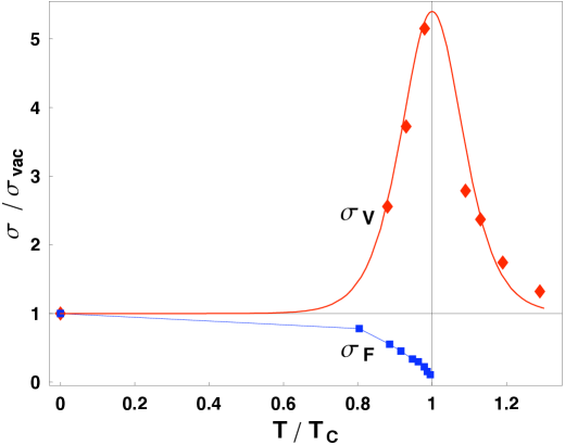
associated with quark pair at distance . We will not show the potentials themselves but just their effective string tensions for both, calculated as a slope of the linear part extracted from Kaczmarek_pure_gauge , is shown in Fig.11. The physical difference between the two, first discussed by Zahed and myself Shuryak:2004tx in the context of hadronic spectroscopy at finite , is that corresponds to adiabatically slow motion of the quarks, slow enough to produce maximal entropy possible and reach thermal equilibrium at any . However when quarks are moving with certain velocity away from each other, only a fraction of the maximal entropy can be produced (because of Landau-Zener argument on level crossing): thus the effective potential would be
| (21) |
For relatively rapid motion in which no entropy is produced, , and one returns to . These arguments have been important to discussion of charmonium survival at RHIC as well as say dominance of baryons our_suscept in the near- region seen on the lattice.
The difference between the two potentials is discussed in detail in Liao:2008vj : in short has been related to “supercurrent coil” and to “normal metastable coil”. If so, large peak at of the tension of is related Liao:2007mj ; Liao:2008vj to a peak in “normal” monopole density at . The condenced and normal monopole density needed to accomodate flux tubes with such tensions have been derived in RefsLiao:2007mj ; Liao:2008vj and compared with direct lattice observations of monopoles. The summary of those studies is that metastable flux tubes seem to exist at , changing from stable to metastable around .
IV.3 Production and breaking of the flux tubes
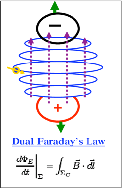
Since the cones and ridges are all created by electrically charged particles propagating in the plasma, they do start with rotating magnetic field related to “dual Faraday” effect shown in Fig.12. While in electric plasma the acceleration happens radially, the magnetic objects are accelerated by the magnetic field. For a relativistic charge those are circles concentrated in a pancake of the width with the spatial distribution
| (22) |
Monopoles (with magnetic charge ) experience instant kick, in the corresponding direction. Its magnitude has no gamma factor and is proportional to the product of electric and magnetic couplings , a Dirac integer. (For elementary quark/gluon electric charge and for Polyakov-t’Hooft monopoles it is just ). Of course electric charge fluctuations can lead to larger charge values as well. This velocity (near-)instantaneously produces a current (or a “coil’) running around the flux. The questions under which condition it is robust enough to contain the field into a static flux tube will be discussed elsewhere.
The interpretation of the linear part of the potential energy coming from the lattice as a metastable flux tube mentioned in the previous subsection, Fig.11, can be used to provide estimates of the absolute amount of energy/matter involved. At the values are astonishingly large: the energy per unit length (tension) reaches at its peak , corresponding to the entropy density of about . One may ask if those parameters can be compatible with observations of the ridges/cone at RHIC.
Let me start addressing this issue from the point of view of energy first. The total energy of the flux tube, or the work done by its tension on the departing charges (large- valence quarks) is . For the M-phase lasting and the proposed V-potential tension, one gets the energy loss of about 25 GeV. Keeping in mind that the total energy of each nucleon in the center of mass is 100 GeV, at RHIC energy used for heavy ions, and that each nucleon has three valence quarks plus sea plus gluons, we conclude that it is comparable to quark total energy. So, if the string would not break, it would be able to transfer valence quarks from the fragmentation region to midrapidity: and we know from experiment that it happens with very small probablity.
The conclusion is then that such strings get broken at time shorter than used in this estimate. This is also known to be true for the usual (vacuum or ) strings: for those the rate of breaking has been phenomenologically extracted from hadron decays, especially of hadrons with large angular momenta (Regge trajectories) and event generators based on the Lund model.
Naively, one might think that “metastable” flux tubes in the M-phase should have lifetime than the vacuum QCD strings. First, their decay can be related not only to (i) the quark pair production, as in vacuum, but also to (ii) just picking up quarks from the ambient matter. However, looking at numbers more closely one finds that it is not nacessarely so.
Quark pair production is described by Schwinger fermion pair production rate (the leading exponent only) in a constant electric field
| (23) |
where is the charged particle mass. The tension scales as , where are electric field and transverse size of the flux tube. There is a universal flux, so , and thus in any change of the tube the field scales as the first power of the tension. If the tension grows by some factor, e.g. as suggested by lattice potential , the field should grow by the same factor. Naively, it would greatly reduce its lifetime111In 1990’s people discussed the so called “color ropes”, as flux tubes with larger flux and thus the field strength, as compared with the vacuum strings. It was done to explain higher strangeness content in AA relative to pp collisions: but the lifetime of such ropes should be smaller than that of the elementary strings. .
Yet the effective mass of quark quasiparticles near is also quite different from “constituent quark mass” in the vaccum () . For example, direct lattice studies Petreczky:2001yp show that at , with perhaps even larger value at . Thus the combination which enters the exponent of the Schwinger formula is not decreasing but rather grows. It suggests a rather counterintuitive conclusion: flux tubes at may have breaking rate than in the vacuum.
The same argument, based on large quark/gluon mass near , leads to small Boltzmann weight which explains small density of these quasiparticles and thus small probablity of a string breaking by picking up free charges.
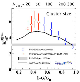
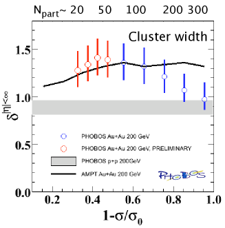
Remarkably, recent RHIC data provided direct experimental indications for enhanced stabilty of the flux tube in matter relative to pp. We will use those from PHOBOS collaboration, which has large rapidity coverage of their silicon detector. Fig.13(a) shows that the number of charged particles in a cluster observed in AuAu collisions (points) is about twice that seen in correlation studies of the pp collisions (shaded horizontal region), so that they reach the size of 6 charged particles (or 9 total). (The exception are central collisions on the right, in which case extensive hadronic after-burning kills the correlations.) The figure (b) shows that the produced clusters are not near-isotropically decaying resonances as in pp, (shaded horizontal region), but are instead more extended in rapidity. This last fact shows their direct relation to the “soft ridge” and flux tubes. Similar CuCu data (not shown) demostrate basically the same clusters, provided the same centrality is taken: this shows that geometry and surface-to-volume ratio is important. Taken together, we interpret those clustering data as direct proof of significant changes in the flux tube decay parameters in AuAu relative to pp: the tubes apparently gets denser and decay less frequently, into larger pieces.
Let me also try to connect the multiplicity in the clusters observed with the entropy as seen in lattice potentials. At the peak the entropy per length is as high as . If this entropy all goes into final pions at freezeout, one can estimate the cluster absolute length. Neglecting the pion mass – that is considering matter to be ideal massless bose gas at freezeout – one find that entropy is 3.6 per particle, or for 10 pions in a cluster. Thus if the decay takes place in the M phase, the cluster corresponds to a string length of 1.2 fm or so. However if the decay rate is small and the string survivies through the M-phase to hadronic phase, the string tension is reduced to the vacuum value 1 GeV/fm, the length corresponding to the observed cluster would be as long as 6 fm. In principle this information can be directly related to the r.m.s. rapidity width of the cluster seen from fig.13(b). We are planning to compare it with some PYTHIA-like simulations to tell whether those clusters can be consistently reproduced.
IV.4 Discussion and predictions
In this section we have suggested two consequences of the small electric screening mass in the M-phase (near region): (i) unscreened bulk electric fields and (ii) metastable (and possibly even relatively long lived) electric flux tube. Taken together, they were called “QGP corona”, with reference to similar phenomena in solar plasma. We had tried to connect this picture with phenomenology of fireball perturbations, namely ridges and cone. Now we would like to speculate further along this line, pointing out some further consequences of the “corona” idea, which can be further tested in experiment.
One direction is related with the predictions of the energy/centrality dependence of the ridges and cones. Already in the introduction we have shown in our sketch of the idea, depicted in Fig.1, we indicated that since the geometry of the M-phase domain is quite different for different collision energies. For RHIC the M-phase sits on the outside of the fireball (Fig.(a)), thus it get a maximal boost from the hydrodynamical expansion and may produce ridges with rather narrow peaks in the azimuthal angle. For much lower energies – corresponding both to the SPS fixed target experiments and planned RHIC scan down) – one should find the M-phase only on the inner part of the fireball (Fig.(b)), which experience little hydro boost if at all. The logical prediction is then that no soft or hard ridges should be observed in this case. Standard modelling using the realistic geometry/density distributions should make those predictions quantitative.
The “cone” is a different story: first of all, those do not rely on overall hydrodynamics and thus may well happen at the very center of the firball and yet be observed. Second important distinction: “cones” are perturbations created by the “away-side” jet, and thus have completely different geometry/timimg. If the trigger jet is surface biased, the away side jet has to fly through rather long path inside fireball, with its length varying roughly between its radius and diameter, 6-12 fm. As one can see from hydro solution, the M-phase starts at time zero at the edge and time about 5 fm/c at the center. Combining two observations together, one would see, that the away-side jet is travelling most of its long path in the M-phase. Furthermore, even at low collision energies, when the M-phase occupies only the central part of the fireball, this conclusion is still fulfilled. The prediction then is that “cones” should not show very strong dependence on collision energy and centrality, in contrast to ridges.
Let us now see how these ideas confront the available data. SPS experiments – CERES and NA49 – have not seen anything like ridges. The centrality and energy dependence of RHIC data we shave shown in Fig.6 do indeed suggest that this phenomenon is disappearing rather rapidly. On the other hand, both CERES and NA49 observe away-side structures which are remarcably similar to RHIC data on the away-side, see review by Harald Appelsh user at the workshop cathie_workshop . We conclude that the picture in which ridges originate from spacial part of the “QGP corona”, while cones are from its temporal part, at times 5-10 fm, is in qualitative agreement with the data.
Finally, let me indicate one more direction of future studies: possible role of the unscreened electric fields in the M-phase in early-time hydro evolution. The pressure of the field, adding to (very low) pressure of the M-phase may help to start hydro a bit earlier and help explain the HBT puzzle. Some studies of the kind (but with non-equilibrium fields rather than DMHD ones) have been made in Ref. Vredevoogd:2008id .
V Conclusions
In summary, we discussed two scenarios of the evolution of extra energy/matter deposited by some fluctuations on top of the “Little bang”. In the scenario (A) we solved equations for propagation of sound with variable speed of sound in expanding matter, using the Hubble flow approximation. We have found that the rapid drop of the sound velocity in the “mixed” phase generates the secondary wave, which under certain conditions may be brighter and smaller in size, and thus is much better candidate for the observed “cone” and “ridges”. However this effect strongly depends on how sharply the speed of sound changes near , with the secondary wave being washed away if changes in the speed of sound gets are too smooth.
In the scenario (B) we assumed that electric field remains unscreened for the duration of the M-phase (near ) and used dual Magnetohydrodynamics. We also found a potential for two expanding cylinders/cones. Furthermore, the speed of one mode can be zero which means that the flux tube of electric gauge field can be pressure- stabilized, by a (metastable) “coil” or current by magnetic charges in plasma. We have argued that this phenomenon is likely to stabilize the flux tubes in the near-Tc region, approximately at . However this temperature interval does not account to all the time of the “Little Bang” at RHIC energies. Presumably the “coil” effect is still present at higher , partially reducing the tube expansion.
For the readers who may be surprised by similarity of the “double cones”, let us remind that similar phenomena are well known in other fields of physics and may appear for multiple reason. In particular, in “dusty” strongly coupled electrodynamic plasmas double Mach cones have been experimentally observed (see e.g.dusty ): in this case these are sound and “shear” or hydroelastic modes which generate them. (Perhaps this option can lead to a “scenario C” not yet considered.)
The very fact that we discuss two competing scenario should tell the reader that at the moment it is hard to tell whether they are robust enough to survive further scrutiny and explain pertinent observations. The “acoustical solution” is not quite robust, it does work only for rather sharp QCD transition which current lattice data do not support. Survival of electric field in the QGP corona is to be studied more, as well as presence of metastable flux tubes. Clearly more theoretical work is needed, including dedicated lattice studies of both monopoles and speed of sound. As far as experiment is concerned, it would be highly important to insure planning so that that jet correlations in question can be followed with sufficient accuracy during the planned RHIC scan toward the lower collision energies. Changing the collision energy one changes the timing of the fireball eras, in a predictable manner, thus for the phenomena we proposed some quantitative predictions can be worked out and tested.
Having said that, we emphasize that those theoretical and experimental studies seem to be very much justified as both may potentially become important discoveries. If the “acoustic scenario” (A) is the explanation, it would be a direct experimental signature of sharp quasi-1st-order QCD phase transition. If the DHMD scenario (B) would be confirmed, it would be quite significant finding, confirming reality of “QGP corona” in which physics is different from what it is inside, as much as it is on the Sun. It will be a big boost to “magnetic scenario” for the near- region Liao_ES_mono ; Chernodub:2006gu .
Acknowledgments. The author indebted to his collaborators (and former students), JinFeng Liao and Jorge Casalderrey-Solana, with whom the development of some of these ideas have been made. I am also indepteed to Larry McLerran and Raju Venugopalan, who attracted his attention to the soft ridge problem, to participants of the correlation workshop cathie_workshop for illuminating discussions, and also to G.Stephens for his explanation of PHOBOS correlation data. This work was supported in parts by the US-DOE grant DE-FG-88ER40388.
References
- (1) D. Teaney, J. Lauret and E. V. Shuryak, Phys. Rev. Lett. 86, 4783 (2001) “A hydrodynamic description of heavy ion collisions at the SPS and RHIC,” arXiv:nucl-th/0110037.
- (2) T. Hirano, Acta Phys. Polon. B 36, 187 (2005)
- (3) C. Nonaka and S. A. Bass, Phys. Rev. C 75, 014902 (2007)
- (4) P. Romatschke and U. Romatschke, Phys. Rev. Lett. 99, 172301 (2007)
- (5) K. Dusling and D. Teaney, Phys. Rev. C 77, 034905 (2008)
- (6) U. W. Heinz and H. Song, J. Phys. G 35, 104126 (2008)
- (7) J. Casalderrey-Solana and E. V. Shuryak, arXiv:hep-ph/0511263.
- (8) J. Liao and E. Shuryak, Phys. Rev. C 77, 064905 (2008)
- (9) J. Liao and E. Shuryak, arXiv:0804.4890 [hep-ph].
- (10) L. D. McLerran and R. Venugopalan, Phys. Rev. D 49, 2233 (1994) [arXiv:hep-ph/9309289].
- (11) E. V. Shuryak, Sov. Phys. JETP 47, 212 (1978) [Zh. Eksp. Teor. Fiz. 74, 408 (1978)].
- (12) S. Mandelstam, Phys. Rept. 23, 245 (1976); G. ’t Hooft, “Topology Of The Gauge Condition And New Confinement Phases In Nonabelian Nucl. Phys. B 190, 455 (1981).
- (13) A. M. Polyakov, Phys. Lett. B 72, 477 (1978).
- (14) J. Liao and E. Shuryak, Phys. Rev. C 75, 054907 (2007) Phys. Rev. Lett. 101, 162302 (2008)
- (15) M. N. Chernodub and V. I. Zakharov, Phys. Rev. Lett. 98, 082002 (2007) [arXiv:hep-ph/0611228].
- (16) A. Nakamura, T. Saito and S. Sakai, Phys. Rev. D 69, 014506 (2004) [arXiv:hep-lat/0311024].
- (17) C. Ratti and E. Shuryak, Phys. Rev. D 80, 034004 (2009) [arXiv:0811.4174 [hep-ph]].
- (18) J.Adams et al (STAR collaboration) PRL 95 (2005) 152301
- (19) S.S.Adler et al (PHENIX collaboration) PRL 97 (2006) 052301
- (20) J.Putschke, Talk at Quark Matter 2006 (for STAR collaboration), Shanghai, Nov.2006. J.Phys.G: Nucl.Part.Phys.34 (2007) S679
- (21) J. Adams et al. [STAR Collaboration], J. Phys. G 32, L37 (2006) [arXiv:nucl-ex/0509030].
- (22) M.Daugherity (for the STAR coll.), Anomalous centrality variation…, QM08, J.Phys.G.Nucl/Part.Phys. 35 (2008) 104090
- (23) G. I. Veres et al. [PHOBOS Collaboration], arXiv:0806.2803 [nucl-ex].
- (24) CATHIE workshop “Critical assessment of theory and experiments on correlations at RHIC, Feb.25-26, BNL. http://www.bnl.gov/cathie-riken
- (25) G.S.F.Stephans (Phobos collaboration) talk at AGS/RHIC Users meeting, June 2009, see also Phys. Rev. C75(2007)054913.arXiv: 0812.1172
- (26) J. Casalderrey-Solana, E. V. Shuryak and D. Teaney, J. Phys. Conf. Ser. 27, 22 (2005) [Nucl. Phys. A 774, 577 (2006)] L. M. Satarov, H. Stoecker and I. N. Mishustin, Phys. Lett. B 627, 64 (2005)
- (27) E. V. Shuryak, Phys. Rev. C 76, 047901 (2007) [arXiv:0706.3531 [nucl-th]].
- (28) S. A. Voloshin, Phys. Lett. B 632, 490 (2006) [arXiv:nucl-th/0312065].
- (29) A. Dumitru, F. Gelis, L. McLerran and R. Venugopalan, Nucl. Phys. A 810, 91 (2008) [arXiv:0804.3858 [hep-ph]].
- (30) S. Gavin, L. McLerran and G. Moschelli, Phys. Rev. C 79, 051902 (2009) [arXiv:0806.4718 [nucl-th]].
- (31) J. Liao and E. Shuryak, Phys. Rev. Lett. 102, 202302 (2009)
- (32) E. Shuryak, Prog. Part. Nucl. Phys. 62, 48 (2009)
- (33) L.D.Landau and E.M.Lifshitz, Theoretical Physics, volume VIII, Electrodynamics of continuous media. volume 8 of Landau-Lifshitz course, Academic Press.
- (34) M. Baker, arXiv:hep-ph/9609269.
- (35) G. S. Bali, arXiv:hep-ph/9809351.
- (36) E. V. Shuryak and I. Zahed, Phys. Rev. D 70, 054507 (2004)
- (37) J. Liao and E. V. Shuryak, Phys. Rev. D 73, 014509 (2006)
- (38) A. D’Alessandro and M. D’Elia, arXiv:0711.1266 [hep-lat].
- (39) O. Kaczmarek and F. Zantow, Phys. Rev. D 71, 114510 (2005)
- (40) P. Petreczky, F. Karsch, E. Laermann, S. Stickan and I. Wetzorke, Nucl. Phys. Proc. Suppl. 106, 513 (2002)
- (41) J. Vredevoogd and S. Pratt, arXiv:0810.4325 [nucl-th].
- (42) G. I. Veres et al. [PHOBOS Collaboration], arXiv:0806.2803 [nucl-ex].
- (43) O. Kaczmarek, F. Karsch, E. Laermann and M. Lutgemeier, Phys. Rev. D 62, 034021 (2000) O. Kaczmarek, F. Karsch, P. Petreczky and F. Zantow, Phys. Lett. B 543, 41 (2002) O. Kaczmarek, F. Karsch, P. Petreczky and F. Zantow, Nucl. Phys. Proc. Suppl. 129, 560 (2004)
- (44) V.Nosenko et al, Phys.Rev.E 68, 056409 (2003)