Cis-Regulatory Modules Drive Dynamic Patterns of a Multicellular System

Abstract

How intracellular and extracellular signals are integrated by transcription factors is essential for understanding complex cellular patterns at the population level. In this Letter, by using a synthetic genetic oscillator coupled to a quorum-sensing apparatus, we propose an experimentally feasible cis-regulatory module (CRM) which performs four possible logic operations (ANDN, ORN, NOR and NAND) of input signals. We show both numerically and theoretically that these different CRMs drive fundamentally different dynamic patterns, such as synchronization, clustering and splay state.

Biological organisms possess an enormous repertoire of genetic responses to ever-varying combinations of cellular and environmental signals BookDavidson01 ; BookAlon06 . Such a repertoire is typically encoded in complex regulatory networks, and affects patterning, differentiation and growth. At the heart of these networks are cis-regulatory modules (CRMs), which contain a cluster of binding sites for transcription factors (TFs) and determine the place and timing of gene action within the network. Both deciphering the codes and elucidating the functions of CRMs involved in various developmental processes are a major challenge in biology.

It has been shown that CRMs can perform an elaborate computation at the individual gene level: the transcription rate of a gene depends on the active concentration of each of inputs Buchler03 ; PlosComputBiol06 ; Mangan03 ; Setty03 ; PlosBiol06 . On the other hand, cells live in a complex environment and can sense many different signals, in particular those from neighboring cells. Therefore, at the multicell level CRMs need to integrate intracellular and extracellular signals so as to coordinate gene expression. Given that cells are frequently subject to chemical signals from neighboring cells, it is worth studying the effect of chemical communication on the dynamic patterns of multicellular systems. Modeling studies, for example, have shown that a population of repressilators coupled to quorum sensing can work as a macroscopic genetic clocks Garcia-Ojalvo04 . In that study, two input signals (i.e., two TFs) regulate a target gene independently. TFs, however, are often integrated in a combinatorial logic manner, and moreover such a combination may take different forms Buchler03 ; PlosComputBiol06 ; Mangan03 ; Setty03 ; PlosBiol06 . From views of evolutionism, CRMs are changeable, e.g., cis-regulatory mutations AWGregory07 . Such a mutation constitutes an important part of the genetic basis for adaptation. A naturally arising question is how the changes of CRMs affect cellular patterns of populations of genetic oscillators. We address this question by designing a multicellular network with a CRM consisting of repressilators Repressilator coupled to quorum sensing Garcia-Ojalvo04 ; McMillen02 ; Fuqua96 in Escherichia coli. In contrast to the previous studies Garcia-Ojalvo04 ; McMillen02 that numerically showed that coupled genetic oscillators can demonstrate synchronous behaviors, we both numerically and theoretically show that different signal integration (ANDN, ORN, NOR, NAND type of responses) leads to fundamentally different properties, such as synchronization, clustering, and splay state. Our results indicate that the CRM has a significant influence on the mode of cellular patterns.

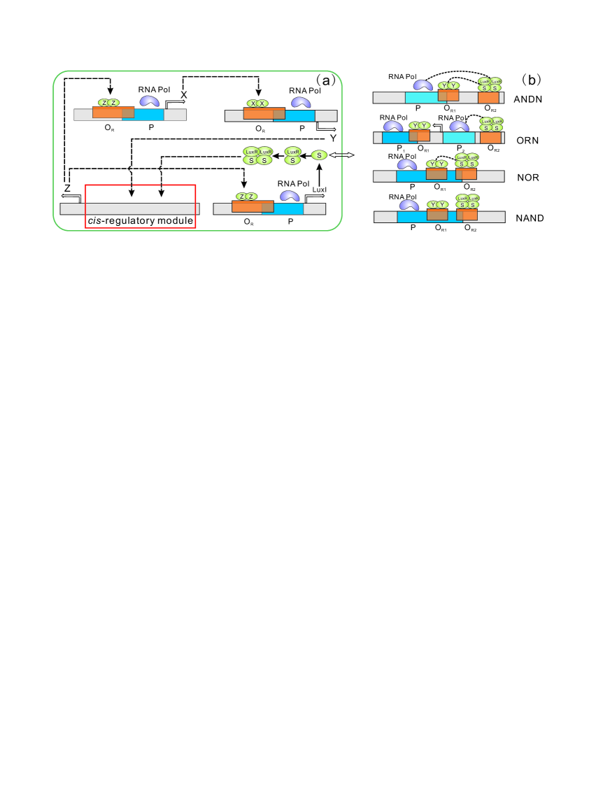
Figure 1: (color). (a) The schematic diagram of a multicellular system with a cis-regulatory module (CRM). Three transcriptional repressors (X, Y, Z) inhibit one another in a cyclic way. The gene luxI from the LuxI/LuxR module first synthesizes a small molecule S. Both S and LuxR then form a hetero-tetramer complex. The dimer of Y and the complex co-regulate the target gene, thus carrying out the function of a CRM (symbolled by the empty box). The right bidirectional arrow indicates that S can freely diffuse through the cellular membrane. (b) Four cis-regulatory constructs for implementations of four different logic functions. From top to bottom is ANDN, ORN, NOR and NAND, respectively. In ANDN, the activator S is unable to act if the repressor Y is bound to the promoter; In ORN, the CRM is constructed using a weak promoter and a strong promoter, where the activator S is able to act if the repressor Y is bound to the promoter; In NOR, two repressors S and Y produce the full repression cooperatively; In NAND, the promoter is regulated exclusively by two repressors. In (a) and (b), P and O_R denote the promoter (dark blue box for the strong promoter and light blue box for the weak promoter) and the operator site (jacinth box) respectively, and the RNA Pol represents RNA polymerase. We use offset and overlapping boxes to indicate the mutual repression and the dashed lines to indicate the cooperative interaction.

A multicellular network under investigation is schematically shown in Fig. 1(a). In such a network, the signaling molecule (S) carries out the information exchange between cells and regulates the expression of a target gene through a CRM. The S and the TF (Y) first bind to specific DNA sequences of the CRM, and then co-regulate the expression of the gene in a combinatorial scheme. In theory, this type of CRM can perform eight different cis-regulatory input functions (CRIFs) PlosComputBiol06 , but limited by the cyclic repression structure of repressilator, we have only four types of CRIFs: ANDN, ORN, NOR and NAND (see Ref. Supp for exact explanations). Figure 1 (b) gives the detailed regulation scheme of every CRM.

Based on the biochemical reactions given in Table 1 and defining the rescaled concentrations as our dynamical variables, the dimensionless equations of intracellular dynamics are described as

$$\frac{d{\bf X}_{i}}{dt} = {\bf F}({\bf X}_{i},S_{i})\,,$$ (1)

$$\frac{dS_{i}}{dt} = E({\bf X}_{i},S_{i})+\eta(S_{e}-S_{i})\,,$$ (2)

where subscript $i$ represents cell $i$ ($=1,2,\cdots,N$), and ${\bf X}_{i}=(x_{i},\,y_{i},\,z_{i},\,X_{i},\,Y_{i},\,Z_{i})^{\rm T}$ with $x_{i}$, $y_{i}$ and $z_{i}$ standing for three mRNA concentrations, and $X_{i}$, $Y_{i}$ and $Z_{i}$ for three protein concentrations. $S_{i}$ represents the concentration of the signaling molecule inside the $i$th cell whereas $S_{e}$ does the concentration of the signal in the extracellular environment. Because of the fast diffusion of the extracellular signal compared to the repressilator period, $S_{e}$ can be assumed to be in the quasi-steady state, leading to $S_{e}=\frac{Q}{N}\sum_{i=1}^{N}S_{i}$, where the parameter $Q$ depends on the cell density in a nonlinear way Garcia-Ojalvo04 . ${\bf F}=(F_{1},F_{2},\ldots,F_{6})^{\rm T}$ with $F_{1}=\frac{\alpha}{1+Z^{n}}-x$, $F_{2}=\frac{\alpha}{1+X^{n}}-y$, $F_{4}=\beta(x-X)$, $F_{5}=\beta(y-Y)$, $F_{6}=\beta(z-Z)$, $E=\gamma X-\delta S$, and

$$F_{3}={\rm CRIF}-z\,,$$ (3)

where we omit subscript $i$ for convenience, and the core function CRIF corresponding to ANDN, ORN, NOR and NAND respectively is listed in the first part of Table 1. The detailed derivation of CRIFs and ${\bf F}$ is put in Ref. Supp . Throughout this Letter, all parameters except for $Q$ are set as $\alpha=204$, $\beta=1$, $\gamma=0.01$, $\delta=1$, $n=2$, $\eta=2$, $\mu=51$, $\nu=204$, $\lambda=1$, which come from experimentally-reasonable settings Supp . Since the numerical results do not depend qualitatively on the cell number, we set $N=120$.

Table 1: Biochemical reactions and cis-regulatory input functions (CRIFs). See Ref. Supp for the derivation of CRIFs, experimental values of parameters (including $\mu$, $\nu$ and $\lambda$ that depend on reaction rates), and meanings of all used symbols.

$$\begin{array}[]{cccccc}\hline\cr\hline\cr\lx@intercol\hfil\mbox{Logic Function}\hfil\lx@intercol&\lx@intercol\hfil\mbox{\hskip 14.22636ptCRIF}\hfil\lx@intercol&\lx@intercol\hfil\hskip 14.22636pt\mbox{Reactions}\hfil\lx@intercol\\ \hline\cr\lx@intercol\hfil\rule[0.0pt]{0.0pt}{16.58774pt}\mbox{ANDN}\hfil\lx@intercol&\lx@intercol\hfil\hskip 14.22636pt\displaystyle\frac{\mu S^{2}}{1+S^{2}+Y^{2}+\lambda S^{2}Y^{2}}\hfil\lx@intercol&\lx@intercol\hfil\hskip 14.22636pt\mbox{\char 172\char 173\char 174\char 176}\hfil\lx@intercol\\[8.61108pt] \lx@intercol\hfil\mbox{ORN}\hfil\lx@intercol&\lx@intercol\hfil\hskip 14.22636pt\displaystyle\frac{\mu S^{2}+\nu}{1+S^{2}+Y^{2}}\hfil\lx@intercol&\lx@intercol\hfil\hskip 14.22636pt\mbox{\char 172\char 174\char 175\char 176}\hfil\lx@intercol\\[8.61108pt] \lx@intercol\hfil\mbox{NOR}\hfil\lx@intercol&\lx@intercol\hfil\hskip 14.22636pt\displaystyle\frac{\nu}{1+S^{2}+Y^{2}+\lambda S^{2}Y^{2}}\hfil\lx@intercol&\lx@intercol\hfil\hskip 14.22636pt\mbox{\char 172\char 173\char 174\char 175}\hfil\lx@intercol\\[8.61108pt] \lx@intercol\hfil\mbox{NAND}\hfil\lx@intercol&\lx@intercol\hfil\hskip 14.22636pt\displaystyle\frac{\nu}{1+S^{2}+Y^{2}}\hfil\lx@intercol&\lx@intercol\hfil\hskip 14.22636pt\mbox{\char 172\char 174\char 175}\hfil\lx@intercol\\[8.61108pt] \hline\cr\lx@intercol\mbox{\hskip 12.80365ptFast Reactions}\hfil\lx@intercol&\lx@intercol\mbox{\hskip 19.91684ptSlow Reactions}\hfil\lx@intercol\\ \hline\cr\lx@intercol\left.\begin{array}[]{l}2{\rm X}\overset{K_{1}}{\underset{}{\rightleftharpoons}}{\rm X}_{2};2{\rm Y}\overset{K_{2}}{\underset{}{\rightleftharpoons}}{\rm Y}_{2}\\[0.0pt] 2{\rm Z}\overset{K_{3}}{\underset{}{\rightleftharpoons}}{\rm Z}_{2};2{\rm C}\overset{K_{4}}{\underset{}{\rightleftharpoons}}{\rm C}_{2}\\[-4.73611pt] {\rm S}+{\rm LuxR}\overset{K_{5}}{\underset{}{\rightleftharpoons}}{\rm C}\\[-4.73611pt] {\rm D}^{Y}+{\rm X}_{2}\overset{K_{6}}{\underset{}{\rightleftharpoons}}{\rm D}_{X}^{Y}\\[-4.73611pt] {\rm D}^{Z}+{\rm Y}_{2}\overset{K_{7}}{\underset{}{\rightleftharpoons}}{\rm D}_{Y}^{Z}\\[-4.73611pt] {\rm D}^{X}+{\rm Z}_{2}\overset{K_{8}}{\underset{}{\rightleftharpoons}}{\rm D}_{Z}^{X}\\[-4.73611pt] {\rm D}^{Z}+{\rm C}_{2}\overset{K_{9}}{\underset{}{\rightleftharpoons}}{\rm D}_{C}^{Z}\\[-4.73611pt] {\rm D}^{L}+{\rm Z}_{2}\overset{K_{10}}{\underset{}{\rightleftharpoons}}{\rm D}_{Z}^{L}\end{array}\right\}\mbox{\char 172}\hfil\lx@intercol&\lx@intercol\left.\begin{array}[]{l}{\rm D}^{X}\overset{k_{X}}{\rightharpoonup}{\rm D}^{X}+{\rm mRNA}_{X}\\[1.29167pt] {\rm D}^{Y}\overset{k_{Y}}{\rightharpoonup}{\rm D}^{Y}+{\rm mRNA}_{Y}\\[1.29167pt] {\rm D}^{L}\overset{k_{L}}{\rightharpoonup}{\rm D}^{L}+{\rm mRNA}_{L}\\[1.29167pt] {\rm L}\overset{c}{\rightharpoonup}{\rm L}+{\rm S};{\rm S}\overset{d_{S}}{\rightharpoonup}\varnothing\\[1.29167pt] {\rm mRNA}_{I}\overset{t_{I}}{\rightharpoonup}{\rm mRNA}_{I}+I\\[1.29167pt] {\rm mRNA}_{I}\overset{e_{I}}{\rightharpoonup}\varnothing\\[1.29167pt] {\rm I}\overset{d_{I}}{\rightharpoonup}\varnothing\\[1.29167pt] \small{\mbox{(I = X, Y, Z, L)}}\end{array}\right\}\mbox{\char 174}\hfil\lx@intercol\\[-3.01385pt] \lx@intercol\begin{array}[]{l}{\rm D}_{C}^{Z}+{\rm Y}_{2}\overset{K_{11}}{\underset{}{\rightleftharpoons}}{\rm D}_{CY}^{Z}\\[-4.30554pt] {\rm D}_{Y}^{Z}+{\rm C}_{2}\overset{K_{12}}{\underset{}{\rightleftharpoons}}{\rm D}_{YC}^{Z}\end{array}\hskip 7.11317pt\Bigg{\}}\hskip 2.84544pt\mbox{\char 173}\hfil\lx@intercol&\lx@intercol\begin{array}[]{l}{\rm D}^{Z}\overset{k_{Z}}{\rightharpoonup}{\rm D}^{Z}+{\rm mRNA}_{Z}\hskip 15.07993pt\big{\}}\hskip 2.56064pt\mbox{\char 175}\\ {\rm D}_{C}^{Z}\overset{fk_{Z}}{\rightharpoonup}{\rm D}_{C}^{Z}+{\rm mRNA}_{Z}\hskip 10.52737pt\big{\}}\hskip 2.56064pt\mbox{\char 176}^{\S}\end{array}\hfil\lx@intercol\\[0.0pt] \hline\cr\hline\cr\lx@intercol\scriptsize{\mbox{${}^{\S}$ In ORN, $k_{Z}$ in \char 176 differs from that in \char 175 due to different promotors.}}\hfil\lx@intercol\end{array}$$

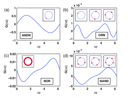
Figure 2: (color). Different cis-regulatory modules drive different cellular patterns. Insets display instantaneous distributions of phases of the oscillators for a fixed $Q=0.5$: (a) 1-cluster state (complete synchronization) for ANDN; (b) 1-, 2- and 3-cluster states for ORN; (c) splay state for NOR; (d) 3-, 4- and 5-cluster states for NAND (the corresponding time courses of all clustering figures are put in the supporting material Ref. Supp ). The function $G(\Delta\phi)$ determines the coupling mode: attractive coupling for ANDN and ORN (due to $G^{\prime}(0)>0$) and repulsive coupling for NOR and NAND (due to $G^{\prime}(0)<0$). Here, the different clusterings arise from different initial phases.

We are interested in the influence of four possible CRIFs on cellular patterns. The results shown in the insets of Fig. 2 indicate that these different CRMs drive fundamentally different dynamic patterns. Specifically, in the case of ANDN, for arbitrarily chosen initial conditions we observe complete synchronization (1-cluster) only, similar to that shown in Refs. Garcia-Ojalvo04 ; McMillen02 ; APikovskyBook01 . This pattern indicates that a specific CRM would combine intracellular and intercellular signals to coordinate the gene expressions in a uniform way at the population level. Interestingly in the case of ORN, we find that different initial conditions lead to three kinds of dynamic patterns: 1-cluster, 2-cluster and 3-cluster balancedcluster . Similar phenomena were also found in a chemical system Kiss05 ; AFTaylor08 . In the case of NOR, however, neither synchronization nor clustering is observed, but an interesting phenomenon that all cells are staggered equally in time, i.e., so-called splay state, is found for the first time in a cell population although the similar phenomenon was also detected experimentally in a multimode laser system Splay . Finally, in the case of NAND, we also observe three types of clusterings at the scattered initial states: 3-, 4- and 5-clusters Ullner07 ; Golomb92 . The complete synchronization, however, never occurs in this case.

To understand and interpret the above interesting patterns, we have performed an analytical study of the system in the phase model description BookKuramoto84 , which holds in a weak coupling case. In this description, we first rewrite Eq. (2) as the following symmetric form of coupling

$$\frac{dS_{i}}{dt}=E({\bf X}_{i},S_{i})-\eta(1-Q)S_{i}+\frac{1}{N}\sum^{N}_{j=1}\eta Q(S_{j}-S_{i})\,.$$ (4)

Then, for convenience the system consisting of both Eq. (1) and the equation

$$\frac{dS_{i}}{dt}=E({\bf X}_{i},S_{i})-\eta(1-Q)S_{i}$$ (5)

is called as auxiliary system, which is assumed to generate a sustained oscillation. For a weak coupling, the Kuramoto phase reduction method BookKuramoto84 gives

$$\frac{d\phi_{i}}{dt}=\omega_{i}+\frac{1}{N}\sum^{N}_{j=1}H_{ij}(\phi_{j}-\phi_{i})\,,$$ (6)

where $\phi_{i}$ and $\omega_{i}$ stand for the phase and frequency of the auxiliary system, respectively. $H_{ij}(\Delta\phi)$ represents the interaction function with respect to the phase difference $\Delta\phi=\phi_{j}-\phi_{i}$ between two cells,

$$H_{ij}(\phi_{j}-\phi_{i})=\frac{1}{2\pi}\int_{0}^{2\pi}Z(\theta)\cdot p(\phi_{j}-\phi_{i}+\theta)d\theta$$ (7)

which can be calculated numerically Ermentrout91 , where $Z(\theta)$, a phase response function characterizing the phase advance per unit perturbation, is a $2\pi$-period function, and $p=(0,0,0,0,0,0,\eta Q(S_{j}-S_{i}))^{\rm T}$. Below we will omit subscripts $i$ and $j$ for convenience. From $H(\Delta\phi)$, we introduce a function: $G(\Delta\phi)=H(\Delta\phi)-H(-\Delta\phi)$, to determine the mode of coupling. If $G(\Delta\phi)$ exhibits a positive slope at $\Delta\phi=0$, i.e, $G^{\prime}(0)>0$, the coupling is phase-attractive; If $G^{\prime}(0)<0$, the coupling is phase-repulsive. Therefore, Fig. 2 implies that the CRMs in the cases of ANDN and ORN correspond to the phase-attractive coupling whereas those in the cases of NOR and NAND correspond to the phase-repulsive coupling. Such an approach based on the sign of $G^{\prime}(0)$ that depends generally on the intrinsic dynamics of the uncoupled oscillator and on the interaction between the oscillators is more effective than that of directly observing the network topology in determining the mode of weak coupling Ullner07 , especially in the case of complex network architectures.

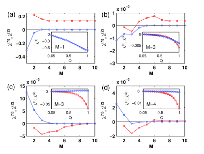
Figure 3: (color). Eigenvalues associated with intra-cluster fluctuations ($\lambda^{(1)}$: blue circle) and the maximal real part of non-zero eigenvalues associated with inter-cluster fluctuations ($\lambda^{(2)}$: red square) as a function of the number of balanced clusters ($M$) for a fixed $Q=0.5$ in the case of: (a) ANDN; (b) ORN; (c) NOR and (d) NAND. Insets: the dependence relation of $\lambda^{(1)}$ and $\lambda^{(2)}$ on the parameter ($Q$) for a particular clustering as indicated.

One cannot, however, obtain knowledge about clustering from the sign of $G^{\prime}(0)$. Since we are interested mainly in balanced clusters balancedcluster , we next employ Okuda’s approach to determine the stability of such clusters Okuda93 . In that method, we need to calculate two kinds of eigenvalues: one is associated with intra-cluster fluctuations and the other with inter-cluster fluctuations, which are denoted by $\lambda_{p}$ and $\lambda_{q}$ (see the caption of Fig. 3) respectively, where $M\leq p\leq N-1$ and $0\leq q\leq M-1$ with $M$ being the number of clusters presumptively. For convenience, denote by $\lambda^{(1)}$ and $\lambda^{(2)}$ the $N-M$ same eigenvalues $\lambda_{p}$ and the maximum of the the real parts of ($M-1$) non-zero eigenvalues $\lambda_{q}$, respectively. Then, the stability of clusterings can be determined by the signs of $\lambda^{(1)}$ and $\lambda^{(2)}$. Specifically, the clustering is stable if both $\lambda^{(1)}$ and $\lambda^{(2)}$ are negative, and unstable if $\lambda^{(2)}$ is positive. In addition, if $\lambda^{(1)}$ is positive and $\lambda^{(2)}$ is negative, and further if $M=N$, the $M$-cluster (i.e., the splay state) are also stable. The dependence of $\lambda^{(1)}$ and $\lambda^{(2)}$ on the balanced cluster number $M$ in the cases of four CRIFs is shown in Fig. 3, which further verifies the dynamic patterns shown in Fig. 2. The insets of Fig. 3 show that the parameter $Q$ has the significant influence on the stability of clusterings (even including 1-cluster in Fig. 2(a) and the splay state in Fig. 2(c)) for a particular balanced cluster state, according to the above analysis.

In addition, in order to verify that the above results are of generality, we also investigated the case of genetic relaxation oscillators by using a detailed example studied in Ref.McMillen02 , and found that different CRMs also drive fundamentally different dynamic patters, but different types of CRIFs would lead to different cellular patterns from those in the case of repressilator (due to the paper length, the detailed results are displayed in Supp ).

In summary, using models of synthetic genetic oscillators coupled to quorum sensing, we have shown that different CRMs drive fundamentally different cellular patterns, such as synchronization, clustering, and splay state. Our results imply the following two points: (1) Multicellular organisms possibly evolve into some functional CRMs for particular goals by performing an elaborate computation for input TFs; (2) Genetic network architecture found in synchronous circadian clocks Garcia-Ojalvo04 ; JCDunlap99 might be constrained since the complete synchronization independent of initial conditions takes place only in the case of ANDN type of responses. In particular, our results do suggest possible candidate circuits for synchronous circadian clocks, while excluding others. We expect that our theoretical findings will stimulate further investigations under a more realistic condition involving stochasticity JMRaser05 ; Zhou05 and spatial heterogeneousness Basu05 , which would help us to understand differentiation patterns and natural developmental processes.

We acknowledge the valuable comments and suggestions of anonymous reviewers and the support from NSKF of P. R. of China (No. 60736028).

References

- (1) E. H. Davidson, Genomic Regulatory Systems: Development and Evolution (Academic Press, San Diego, CA, 2001).
- (2) U. Alon, An Introduction to Systems Biology: Design Principles of Biological Circuits (Chapman & Hall/CRC, London, 2006).
- (3) N. E. Buchler, U. Gerland, and T. Hwa, Proc. Natl. Acad. Sci. U.S.A. 100, 5136 (2003).
- (4) R. Hermsen, S. Tans, and P. R. ten Wolde, PLoS Comput. Biol. 2, e164 (2006).
- (5) S. Mangan and U. Alon, Proc. Natl. Acad. Sci. U.S.A. 100, 11980 (2003).
- (6) Y. Setty et al., Proc. Natl. Acad. Sci. U.S.A. 100, 7702 (2003).
- (7) A. E. Mayo et al., PLoS Biol. 4, e45 (2006).
- (8) J. García-Ojalvo, M. B. Elowitz, and S. H. Strogatz, Proc. Natl. Acad. Sci. U.S.A. 101, 10955 (2004).
- (9) A. W. Gregory, Nat Rev Genet. 8, 206 (2007).
- (10) M. B. Elowitz and S. Leibler, Nature (London) 403, 335 (2000).
- (11) D. McMillen et al., Proc. Natl. Acad. Sci. U.S.A. 99, 679 (2002).
- (12) C. Fuqua, S. C. Winans, and E. P. Greenberg, Annu. Rev. Microbiol. 50, 727 (1996).
- (13) Supporting material available upon request.
- (14) A. Pikovsky, M. Rosenblum, and J. Kurths, Synchronization – A Universal Concept in Nonlinear Science (Cambridge University Press, Cambridge, England, 2001).
- (15) Here we consider balanced clusterings only. Other clusterings are possible.
- (16) I. Z. Kiss, Y. Zhai, and J. L. Hudson, Phys. Rev. Lett. 94, 248301 (2005).
- (17) A. F. Taylor et al., Phys. Rev. Lett. 100, 214101 (2008).
- (18) K. Wiesenfeld et al., Phys. Rev. Lett. 65, 1749 (1990); S. Nichols and K. Wiesenfeld, Phys. Rev. A 45, 8430 (1992); S. H. Strogatz and R. E. Mirollo, Phys. Rev. E 47, 220 (1993).
- (19) E. Ullner et al., Phys. Rev. Lett. 99, 148103 (2007).
- (20) D. Golomb et al., Phys. Rev. A 45, 3516 (1992).
- (21) Y. Kuramoto, Chemical Oscillations, Waves and Turbulence (Springer-Verlag, Berlin, 1984).
- (22) G. B. Ermentrout and N. Kopell, J. Math. Biol. 29, 195 (1991).
- (23) K. Okuda, Physica D (Amsterdam) 63, 424 (1993).
- (24) J. C. Dunlap, Cell 96, 271 (1999).
- (25) J. M. Raser and E. K. O’Shea, Science 309, 2010 (2005).
- (26) T. S. Zhou, L. N. Chen, and K. Aihara, Phys. Rev. Lett. 95, 178103 (2005).
- (27) S. Basu et al., Nature (London) 434, 1130 (2005).