Computations Modulo Regular Chains

Abstract

The computation of triangular decompositions involves two fundamental operations: polynomial GCDs modulo regular chains and regularity test modulo saturated ideals. We propose new algorithms for these core operations based on modular methods and fast polynomial arithmetic. We rely on new results connecting polynomial subresultants and GCDs modulo regular chains. We report on extensive experimentation, comparing our code to pre-existing Maple implementations, as well as more optimized Magma functions. In most cases, our new code outperforms the other packages by several orders of magnitude.

Keywords: Fast polynomial arithmetic, regular chain, regular GCD, subresultants, triangular decomposition, polynomial systems.

1 Introduction

A triangular decomposition of a set $F\subset{\mathbf{k}}[x_{1},\ldots,x_{n}]$ is a list of polynomial systems $T_{1},\ldots,T_{e}$, called regular chains (or regular systems) and representing the zero set $V(F)$ of $F$. Each regular chain $T_{i}$ may encode several irreducible components of $V(F)$ provided that those share some properties (same dimension, same free variables, …).

Triangular decomposition methods are based on a univariate and recursive vision of multivariate polynomials. Most of their routines manipulate polynomial remainder sequences (PRS). Moreover, these methods are usually “factorization free”, which explains why two different irreducible components may be represented by the same regular chain. An essential routine is then to check whether a hypersurface $f=0$ contains one of the irreducible components encoded by a regular chain $T$. This is achieved by testing whether the polynomial $f$ is a zero-divisor modulo the so-called saturated ideal of $T$. The univariate vision on regular chains allows to perform this regularity test by means of GCD computations. However, since the saturated ideal of $T$ may not prime, the concept of a GCD used here is not standard.

The first formal definition of this type of GCDs was given by Kalkbrener in [14]. But in fact, GCDs over non-integral domains were already used in several papers [9, 16, 12] since the introduction of the celebrated D5 Principle [7] by Della Dora, Dicrescenzo and Duval. Indeed, this brilliant and simple observation allows one to carry out over direct product of fields computations that are usually conducted over fields. For instance, computing univariate polynomial GCDs by means of the Euclidean Algorithm.

To define a polynomial GCD of two (or more) polynomials modulo a regular chain $T$, Kalkbrener refers to the irreducible components that $T$ represents. In order to improve the practical efficiency of those GCD computations by means of subresultant techniques, Rioboo and the second author proposed a more abstract definition in [23]. Their GCD algorithm is, however, limited to regular chains with zero-dimensional saturated ideals.

While Kalkbrener’s definition cover the positive dimensional case, his approach cannot support triangular decomposition methods solving polynomial systems incrementally, that is, by solving one equation after another. This is a serious limitation since incremental solving is a powerful way to develop efficient sub-algorithms, by means of geometrical consideration. The first incremental triangular decomposition method was proposed by Lazard in [15], without proof nor a GCD definition. Another such method was established by the second author in [22] together with a formal notion of GCD adapted to the needs of incremental solving. This concept, called regular GCD, is reviewed in Section 2 in the context of regular chains. A more abstract definition follows.

Let $\mathbb{B}$ be a commutative ring with unity. Let $P,Q,G$ be non-zero univariate polynomials in ${\mathbb{B}}[y]$. We say that $G$ is a regular GCD of $P,Q$ if the following three conditions hold:

• the leading coefficient of $G$ is a regular element of $\mathbb{B}$,

• $G$ lies in the ideal generated by $P$ and $Q$ in ${\mathbb{B}}[y]$, and

• if $G$ has positive degree w.r.t. $y$, then $G$ pseudo-divides both of $P$ and $Q$, that is, the pseudo-remainders $\mathrm{prem}(P,G)$ and $\mathrm{prem}(Q,G)$ are null.

In the context of regular chains, the ring $\mathbb{B}$ is the residue class ring of a polynomial ring ${\mathbb{A}}:={\mathbf{k}}[x_{1},\ldots,x_{n}]$ (over a field $\mathbf{k}$) by the saturated ideal $\mathrm{sat}(T)$ of a regular chain $T$. Even if the leading coefficients of $P,Q$ are regular and $\mathrm{sat}(T)$ is radical, the polynomials $P,Q$ may not necessarily admit a regular GCD (unless $\mathrm{sat}(T)$ is prime). However, by splitting $T$ into several regular chains $T_{1},\ldots,T_{e}$ (in a sense specified in Section 2) one can compute a regular GCD of $P,Q$ over each of the ring ${\mathbb{A}}/\mbox{$\mathrm{sat}(T_{i})$}$, as shown in [22].

In this paper, we propose a new algorithm for this task, together with a theoretical study and implementation report, providing dramatic improvements w.r.t. previous work [14, 22]. Section 3 exhibits sufficient conditions for a subresultant polynomial of $P,~{}Q\in{\mathbb{A}}[y]$ (regarded as univariate polynomials in $y$) to be a regular GCD of $P,~{}Q$ w.r.t. $T$. Some of these properties could be known, but we could not find a reference for them, in particular when $\mathrm{sat}(T)$ is not radical. These results reduce the computation of regular GCDs to that of subresultant chains, see Section 4 for details.

Since Euclidean-like algorithms tend to densify computations, we consider an evaluation/interpolation scheme based on FFT techniques for computing subresultant chains. In addition, we observe that, while computing triangular decomposition, whenever a regular GCD of $P$ and $Q$ w.r.t. $T$ is needed, the resultant of $P$ and $Q$ w.r.t. $y$ is likely to be computed too. This suggests to organize calculations in a way that the subresultant chain of $P$ and $Q$ is computed only once. Moreover, we wish to follow a successful principle introduced in [20]: compute in ${\mathbf{k}}[x_{1},\ldots,x_{n}]$ instead of ${\mathbf{k}}[x_{1},\ldots,x_{n}]/\mbox{$\mathrm{sat}(T)$}$, as much as possible, while controlling expression swell. These three requirements targeting efficiency are satisfied by the implementation techniques of Section 5.1. The use of fast arithmetic for computing regular GCDs was proposed in [6] for regular chains with zero-dimensional radical saturated ideals. However this method does not meet our other two requirements and does not apply to arbitrary regular chains. We state complexity results for the algorithms of this paper in Sections 5.1 and 5.2.

Efficient implementation is the main objective of our work. We explain in Section 5.3 how we create opportunities for using modular methods and fast arithmetic in operations modulo regular chains, such as regular GCD computation and regularity test. The experimental results of Section 6 illustrate the high efficiency of our algorithms. We obtain speed-up factors of several orders of magnitude w.r.t. the algorithms of [22] for regular GCD computations and regularity test. Our code compares and often outperforms packages with similar specifications in Maple and Magma.

2 Preliminaries

Let $\mathbf{k}$ be a field and let $\mathbf{k}[\mathbf{x}]=\mathbf{k}[x_{1},\ldots,x_{n}]$ be the ring of polynomials with coefficients in $\mathbf{k}$, with ordered variables $x_{1}\prec\cdots\prec x_{n}$. Let ${\overline{\mathbf{k}}}$ be the algebraic closure of $\mathbf{k}$. If $\mathbf{u}$ is a subset of $\mathbf{x}$ then ${\mathbf{k}}(\mathbf{u})$ denotes the fraction field of $\mathbf{k}[\mathbf{u}]$. For $F\subset{\mathbf{k}}[\mathbf{x}]$, we denote by $\langle F\rangle$ the ideal it generates in ${\mathbf{k}}[\mathbf{x}]$ and by $\sqrt{\langle F\rangle}$ the radical of $\langle F\rangle$. For $H\in\mathbf{k}[\mathbf{x}]$, the saturated ideal of $\langle F\rangle$ w.r.t. $H$, denoted by $\langle F\rangle:H^{\infty}$, is the ideal $\{Q\in\mathbf{k}[\mathbf{x}]\mid\exists m\in\mathbb{N}\text{ s.t. }H^{m}Q\in\langle F\rangle\}.$ A polynomial $P\in\mathbf{k}[\mathbf{x}]$ is a zero-divisor modulo $\langle F\rangle$ if there exists a polynomial $Q$ such that $PQ\in\langle F\rangle$, and neither $P$ nor $Q$ belongs to $\langle F\rangle$. The polynomial $P$ is regular modulo $\langle F\rangle$ if it is neither zero, nor a zero-divisor modulo $\langle F\rangle$. We denote by $V(F)$ the zero set (or algebraic variety) of $F$ in ${\overline{\mathbf{k}}}^{n}$. For a subset $W\subset{\overline{\mathbf{k}}}^{n}$, we denote by $\overline{W}$ its closure in the Zariski topology.

2.1 Regular chains and related notions

Main variable and initial. If $P\in{\mathbf{k}}[\mathbf{x}]$ is a non-constant polynomial, the largest variable appearing in $P$ is called the main variable of $P$ and is denoted by $\mathrm{mvar}(P)$. The leading coefficient of $P$ w.r.t. $\mathrm{mvar}(P)$ is its initial, written $\mathrm{init}(P)$ whereas lc$(P,v)$ is the leading coefficient of $P$ w.r.t. $v\in\mathbf{x}$.

Triangular Set. A subset $T$ of non-constant polynomials of ${\mathbf{k}}[\mathbf{x}]$ is a triangular set if the polynomials in $T$ have pairwise distinct main variables. Denote by $\mathrm{mvar}(T)$ the set of all $\mathrm{mvar}(P)$ for $P\in T$. A variable $v\in\mathbf{x}$ is algebraic w.r.t. $T$ if $v\in\mbox{$\mathrm{mvar}(T)$}$; otherwise it is free. For a variable $v\in\mathbf{x}$ we denote by $T_{<v}$ (resp. $T_{>v}$) the subsets of $T$ consisting of the polynomials with main variable less than (resp. greater than) $v$. If $v\in\mbox{$\mathrm{mvar}(T)$}$, we denote by $T_{v}$ the polynomial $P\in T$ with main variable $v$. For $T$ not empty, $T_{\rm max}$ denotes the polynomial of $T$ with largest main variable.

Quasi-component and saturated ideal. Given a triangular set $T$ in $\mathbf{k}[\mathbf{x}]$, denote by $h_{T}$ the product of the $\mathrm{init}(P)$ for all $P\in T$. The quasi-component $W({T})$ of $T$ is $V(T)\setminus V(h_{T})$, that is, the set of the points of $V({T})$ which do not cancel any of the initials of ${T}$. We denote by $\mathrm{sat}(T)$ the saturated ideal of $T$, defined as follows: if $T$ is empty then $\mathrm{sat}(T)$ is the trivial ideal $\langle 0\rangle$; otherwise it is the ideal $\langle T\rangle:h_{T}^{\infty}$.

Regular chain. A triangular set $T$ is a regular chain if either $T$ is empty, or $T\setminus\{T_{max}\}$ is a regular chain and the initial of ${T}_{max}$ is regular with respect to $\mathrm{sat}(T\setminus\{T_{max}\})$. In this latter case, $\mathrm{sat}(T)$ is a proper ideal of ${\mathbf{k}}[\mathbf{x}]$. From now on $T\subset{\mathbf{k}}[\mathbf{x}]$ is a regular chain; moreover we write $m=|T|$, $\mathbf{s}=\mbox{$\mathrm{mvar}(T)$}$ and $\mathbf{u}=\mathbf{x}\setminus\mathbf{s}$. The ideal $\mathrm{sat}(T)$ enjoys several properties. First, its zero-set equals $\overline{W(T)}$. Second, the ideal $\mathrm{sat}(T)$ is unmixed with dimension $n-m$. Moreover, any prime ideal ${\mathfrak{p}}$ associated to $\mathrm{sat}(T)$ satisfies ${\mathfrak{p}}\,{\cap}\,{\mathbf{k}}[\mathbf{u}]=\langle 0\rangle$. Third, if $n=m$, then $\mathrm{sat}(T)$ is simply $\langle T\rangle$. Given $P\in{\mathbf{k}}[\mathbf{x}]$ the pseudo-remainder (resp. iterated resultant) of $P$ w.r.t. $T$, denoted by $\mathrm{prem}(P,T)$ (resp. res$(P,T)$) is defined as follows. If $P\in{\mathbf{k}}$ or no variables of $P$ is algebraic w.r.t. $T$, then $\mbox{$\mathrm{prem}(P,T)$}=P$ (resp. $\mbox{{\sf res}$(P,T)$}=P$). Otherwise, we set $\mbox{$\mathrm{prem}(P,T)$}=\mbox{$\mathrm{prem}(R,T_{<v})$}$ (resp. $\mbox{{\sf res}$(P,T)$}=\mbox{{\sf res}$(R,T_{<v})$}$) where $v$ is the largest variable of $P$ which is algebraic w.r.t. $T$ and $R$ is the pseudo-remainder (resp. resultant) of $P$ and $T_{v}$ w.r.t. $v$. We have: $P$ is null (resp. regular) w.r.t. $\mathrm{sat}(T)$ if and only if $\mbox{$\mathrm{prem}(P,T)$}=0$ (resp. $\mbox{{\sf res}$(P,T)$}\neq 0$).

Regular GCD. Let $I$ be the ideal generated by $\sqrt{\mbox{$\mathrm{sat}(T)$}}$ in ${\mathbf{k}}(\mathbf{u})[\mathbf{s}]$. Then ${\mathbb{L}}(T):={\mathbf{k}}(\mathbf{u})[\mathbf{s}]/I$ is a direct product of fields. It follows that every pair of univariate polynomials $P,Q\in{\mathbb{L}}(T)[y]$ possesses a GCD in the sense of [23]. The following GCD notion [22] is convenient since it avoids considering radical ideals. Let $T\subset{\mathbf{k}}[x_{1},\ldots,x_{n}]$ be a regular chain and let $P,Q\in{\mathbf{k}}[\mathbf{x},y]$ be non-constant polynomials both with main variable $y$. Assume that the initials of $P$ and $Q$ are regular modulo $\mathrm{sat}(T)$. A non-zero polynomial $G\in{\mathbf{k}}[\mathbf{x},y]$ is a regular GCD of $P,Q$ w.r.t. $T$ if these conditions hold:

• lc$(G,y)$ is regular with respect to $\mathrm{sat}(T)$;

• there exist $u,v\in{\mathbf{k}}[\mathbf{x},y]$ such that $g-up-vt\in\mbox{$\mathrm{sat}(T)$}$;

• if ${\deg}(G,y)>0$ holds, then $\langle P,Q\rangle\subseteq\mbox{$\mathrm{sat}(T\cup G)$}$.

In this case, the polynomial $G$ has several properties. First, it is regular with respect to $\mathrm{sat}(T)$. Moreover, if $\mathrm{sat}(T)$ is radical and ${\deg}(G,y)>0$ holds, then the ideals $\langle P,Q\rangle$ and $\langle G\rangle$ of ${\mathbb{L}}({T})[y]$ are equal, so that $G$ is a GCD of $(P,Q)$ w.r.t. $T$ in the sense of [23]. The notion of a regular GCD can be used to compute intersections of algebraic varieties. As an example we will use Formula (1) which follows from Theorem 32 in [22]. Assume that the regular chain $T$ is simply $\{R\}$ where $R=\mbox{{\sf res}$(P,Q,y)$}$, for $R\not\in{\mathbf{k}}$, and let $H$ be the product of the initials of $P$ and $Q$. Then, we have:

$$V(P,Q)=\overline{W(R,G)}\ \cup\ V(H,P,Q).$$ (1)

Splitting. Two polynomials $P,Q$ may not necessarily admit a regular GCD w.r.t. a regular chain $T$, unless $\mathrm{sat}(T)$ is prime, see Example $1$ in Section 3. However, if $T$ “splits” into several regular chains, then $P,Q$ may admit a regular GCD w.r.t. each of them. This requires a notation. For non-empty regular chains $T,T_{1},\ldots,T_{e}\subset{\mathbf{k}}[\mathbf{x}]$ we write $T\longrightarrow(T_{1},\ldots,T_{e})$ whenever $\sqrt{\mbox{$\mathrm{sat}(T)$}}=\sqrt{\mbox{$\mathrm{sat}(T_{1})$}}\cap\cdots\cap\sqrt{\mbox{$\mathrm{sat}(T_{e})$}}$, $\mbox{$\mathrm{mvar}(T)$}=\mbox{$\mathrm{mvar}(T_{i})$}$ and $\mbox{$\mathrm{sat}(T)$}\subseteq\mbox{$\mathrm{sat}(T_{i})$}$ hold for all $1\leq i\leq e$. If this holds, observe that any polynomial $H$ regular w.r.t $\mathrm{sat}(T)$ is also regular w.r.t. $\mathrm{sat}(T_{i})$ for all $1\leq i\leq e$.

2.2 Fundamental operations on regular chains

We list below the specifications of the fundamental operations on regular chains used in this paper. The names and specifications of these operations are the same as in the RegularChains library [18] in Maple.

Regularize. For a regular chain $T\subset{\mathbf{k}}[\mathbf{x}]$ and $P$ in ${\mathbf{k}}[\mathbf{x}]$, the operation Regularize$(P,T)$ returns regular chains $T_{1},\ldots,T_{e}$ of ${\mathbf{k}}[\mathbf{x}]$ such that, for each $1\leq i\leq e$, $P$ is either zero or regular modulo $\mathrm{sat}(T_{i})$ and we have $T{\longrightarrow}(T_{1},\ldots,T_{e})$.

RegularGcd. Let $T$ be a regular chain and let $P,Q\in{\mathbf{k}}[\mathbf{x},y]$ be non-constant with $\mbox{$\mathrm{mvar}(P)$}=\mbox{$\mathrm{mvar}(Q)$}\not\in\mbox{$\mathrm{mvar}(T)$}$ and such that both $\mathrm{init}(P)$ and $\mathrm{init}(Q)$ are regular w.r.t. $\mathrm{sat}(T)$. Then, the operation RegularGcd$(P,Q,T)$ returns a sequence $(G_{1},T_{1}),\ldots,(G_{e},T_{e})$, called a regular GCD sequence, where $G_{1},\ldots,G_{e}$ are polynomials and $T_{1},\ldots,T_{e}$ are regular chains of ${\mathbf{k}}[\mathbf{x}]$, such that $T{\longrightarrow}(T_{1},\ldots,T_{e})$ holds and $G_{i}$ is a regular GCD of $P,Q$ w.r.t. $T_{i}$ for all $1\leq i\leq e$.

NormalForm. Let $T$ be a zero-dimensional normalized regular chain, that is, a regular chain whose saturated ideal is zero-dimensional and whose initials are all in the base field $\mathbf{k}$. Observe that $T$ is a lexicographic Gröbner basis. Then, for $P\in{\mathbf{k}}[\mathbf{x}]$, the operation NormalForm$(P,T)$ returns the normal form of $P$ w.r.t. $T$ in the sense of Gröbner bases.

Normalize. Let $T$ be a regular chain such that each variable occurring in $T$ belongs to $\mathrm{mvar}(T)$. Let $P\in{\mathbf{k}}[\mathbf{x}]$ be non-constant with initial $H$ regular w.r.t. $\langle T\rangle$. Assume each variable of $H$ belongs to $\mathrm{mvar}(T)$. Then $H$ is invertible modulo $\langle T\rangle$ and Normalize$(P,T)$ returns NormalForm$(H^{-1}P,T)$ where $H^{-1}$ is the inverse of $H$ modulo $\langle T\rangle$.

2.3 Subresultants

We follow the presentation of [8], [25] and [10].

Determinantal polynomial. Let $\mathbb{B}$ be a commutative ring with identity and let $m\leq n$ be positive integers. Let $M$ be a $m\times n$ matrix with coefficients in $\mathbb{B}$. Let $M_{i}$ be the square submatrix of $M$ consisting of the first $m-1$ columns of $M$ and the $i$-th column of $M$, for $i=m\cdots n$; let $\det{M_{i}}$ be the determinant of $M_{i}$. We denote by dpol$(M)$ the element of ${\mathbb{B}}[y]$, called the determinantal polynomial of $M$, given by

$$\det{M_{m}}y^{n-m}+\det{M_{m+1}}y^{n-m-1}+\cdots+\det{M_{n}}.$$

Note that if dpol$(M)$ is not zero then its degree is at most $n-m$. Let $P_{1},\ldots,P_{m}$ be polynomials of ${\mathbb{B}}[y]$ of degree less than $n$. We denote by mat$(P_{1},\ldots,P_{m})$ the $m\times n$ matrix whose $i$-th row contains the coefficients of $P_{i}$, sorting in order of decreasing degree, and such that $P_{i}$ is treated as a polynomial of degree $n-1$. We denote by dpol$(P_{1},\ldots,P_{m})$ the determinantal polynomial of mat$(P_{1},\ldots,P_{m})$.

Subresultant. Let $P,Q\in{\mathbb{B}}[y]$ be non-constant polynomials of respective degrees $p,q$ with $q\leq p$. Let $d$ be an integer with $0\leq d<q$. Then the $d$-th subresultant of $P$ and $Q$, denoted by $S_{d}(P,Q)$, is

$$\mbox{{\rm dpol}$(y^{q-d-1}P,y^{q-d-2}P,\ldots,P,y^{p-d-1}Q,\ldots,Q)$}.$$

This is a polynomial which belongs to the ideal generated by $P$ and $Q$ in ${\mathbb{B}}[y]$. In particular, $S_{0}(P,Q)$ is res$(P,Q)$, the resultant of $P$ and $Q$. Observe that if $S_{d}(P,Q)$ is not zero then its degree is at most $d$. When $S_{d}(P,Q)$ has degree $d$, it is said non-defective or regular; when $S_{d}(P,Q)\neq 0$ and ${\deg}(S_{d}(P,Q))<d$, $S_{d}(P,Q)$ is said defective. We denote by $s_{d}$ the coefficient of $S_{d}(P,Q)$ in $y^{d}$. For convenience, we extend the definition to the $q$-th subresultant as follows:

$$S_{q}(P,Q)=\left\{\begin{array}[]{ll}\gamma(Q)Q,&\text{if }p>q\text{ or }\mbox{{\rm lc}$(Q)$}\in\mathbb{B}\text{ is regular}\\ \text{undefined},&otherwise\end{array}\right.$$

where $\gamma(Q)=\mbox{{\rm lc}$(Q)$}^{p-q-1}$. Note that when $p$ equals $q$ and lc$(Q)$ is a regular element in $\mathbb{B}$, $S_{q}(P,Q)=\mbox{{\rm lc}$(Q)$}^{-1}Q$ is in fact a polynomial over the total fraction ring of $\mathbb{B}$.

We call specialization property of subresultants the following statement. Let $\mathbb{D}$ be another commutative ring with identity and $\Psi$ a ring homomorphism from $\mathbb{B}$ to $\mathbb{D}$ such that we have $\Psi(\mbox{{\rm lc}$(P)$})\neq 0$ and $\Psi(\mbox{{\rm lc}$(Q)$})\neq 0$. Then we also have

$$S_{d}(\Psi(P),\Psi(Q))=\Psi(S_{d}(P,Q)).$$

Divisibility relations of subresultants. The subresultants $S_{q-1}(P,Q),S_{q-2}(P,Q)$, $\ldots$, $S_{0}(P,Q)$ satisfy relations which induce an Euclidean-like algorithm for computing them. Following [8] we first assume that ${\mathbb{B}}$ is an integral domain. In the above, we simply write $S_{d}$ instead of $S_{d}(P,Q)$, for $d=q-1,\ldots,0$. We write $A\sim B$ for $A,B\in{\mathbb{B}}[y]$ whenever they are associated over fr$(\mathbb{B})$, the field of fractions of $\mathbb{B}$. For $d=q-1,\ldots,1$, we have:

• $S_{q-1}=\mbox{$\mathrm{prem}(P,-Q)$}$, the pseudo-remainder of $P$ by $-Q$,

• if $S_{q-1}\neq 0$, with $e={\deg}(S_{q-1})$, then the following holds: $\mbox{$\mathrm{prem}(Q,-S_{q-1})$}={\mbox{{\rm lc}$(Q)$}}^{(p-q)(q-e)+1}S_{e-1}$,

• if $S_{d-1}\neq 0$, with $e={\deg}(S_{d-1})<d-1$, thus $S_{d-1}$ is defective, and we have

  • ${\deg}(S_{d})=d$, thus $S_{d}$ is non-defective,

  • $S_{d-1}\sim S_{e}$ and ${\mbox{{\rm lc}$(S_{d-1})$}}^{d-e-1}S_{d-1}={s_{d}}^{d-e-1}{S_{e}}$, thus $S_{e}$ is non-defective,

  • $S_{d-2}=S_{d-3}=\cdots=S_{e+1}=0$,

• if $S_{d}$ and $S_{d-1}$ are nonzero, with respective degrees $d$ and $e$, then we have $\mbox{$\mathrm{prem}(S_{d},-S_{d-1})$}={\mbox{{\rm lc}$(S_{d})$}}^{d-e+1}S_{e-1}$,

We consider now the case where $\mathbb{B}$ is an arbitrary commutative ring, following Theorem 4.3 in [10]. If $S_{d},S_{d-1}$ are non zero, with respective degrees $d$ and $e$ and if $s_{d}$ is regular in $\mathbb{B}$ then we have ${\mbox{{\rm lc}$(S_{d-1})$}}^{d-e-1}S_{d-1}={s_{d}}^{d-e-1}{S_{e}}$; moreover, there exists $C_{d}\in{\mathbb{B}}[y]$ such that we have:

$$(-1)^{d-1}\mbox{{\rm lc}$(S_{d-1})$}s_{e}S_{d}+C_{d}S_{d-1}={\mbox{{\rm lc}$(S_{d})$}}^{2}S_{e-1}.$$

In addition $S_{d-2}=S_{d-3}=\cdots=S_{e+1}=0$ also holds.

3 Regular GCDs

Throughout this section, we assume $n\geq 1$ and we consider $P,Q\in{\mathbf{k}}[x_{1},\ldots,x_{n+1}]$ non-constant polynomials with the same main variable $y:=x_{n+1}$ and such that $p:={\deg}(P,y)\geq q:={\deg}(Q,y)$ holds. We denote by $R$ the resultant of $P$ and $Q$ w.r.t. $y$. Let $T\subset{\mathbf{k}}[x_{1},\ldots,x_{n}]$ be a non-empty regular chain such that $R\in\mbox{$\mathrm{sat}(T)$}$ and the initials of $P,Q$ are regular w.r.t. $\mathrm{sat}(T)$. We denote by ${\mathbb{A}}$ and ${\mathbb{B}}$ the rings ${\mathbf{k}}[x_{1},\ldots,x_{n}]$ and ${\mathbf{k}}[x_{1},\ldots,x_{n}]/\mbox{$\mathrm{sat}(T)$}$, respectively. Let $\Psi$ be both the canonical ring homomorphism from ${\mathbb{A}}$ to ${\mathbb{B}}$ and the ring homomorphism it induces from ${\mathbb{A}}[y]$ to ${\mathbb{B}}[y]$. For $0\leq j\leq q$, we denote by $S_{j}$ the $j$-th subresultant of $P,Q$ in ${\mathbb{A}}[y]$.

Let $d$ be an index in the range $1\cdots q$ such that $S_{j}\in\mbox{$\mathrm{sat}(T)$}$ for all $0\leq j<d$. Lemma 3 and Lemma 4 exhibit conditions under which $S_{d}$ is a regular GCD of $P$ and $Q$ w.r.t. $T$. Lemma 1 and Lemma 2 investigate the properties of $S_{d}$ when $\mathrm{lc}(S_{d},y)$ is regular modulo $\mathrm{sat}(T)$ and $\mathrm{lc}(S_{d},y)\in\mbox{$\mathrm{sat}(T)$}$ respectively.

Lemma 1

If $\mathrm{lc}(S_{d},y)$ is regular modulo $\mathrm{sat}(T)$, then the polynomial $S_{d}$ is a non-defective subresultant of $P$ and $Q$ over $\mathbb{A}$. Consequently, $\Psi(S_{d})$ is a non-defective subresultant of $\Psi(P)$ and $\Psi(Q)$ in $\mathbb{B}[y]$.

Proof. When $d=q$ holds, we are done. Assume $d<q$. Suppose $S_{d}$ is defective, that is, $\deg(S_{d},y)=e<d$. According to item $(r_{e})$ in the divisibility relations of subresultants, there exists a non-defective subresultant $S_{d+1}$ such that

$$\mbox{{\rm lc}$(S_{d},y)$}^{d-e}S_{d}=s_{d+1}^{d-e}S_{e},$$

where $s_{d+1}$ is the leading coefficient of $S_{d+1}$ in $y$. By our assumptions, $S_{e}$ belongs to $\mathrm{sat}(T)$, thus $\mbox{{\rm lc}$(S_{d},y)$}^{d-e}S_{d}\in\mbox{$\mathrm{sat}(T)$}$ holds. It follows from the fact lc$(S_{d},y)$ is regular modulo $\mathrm{sat}(T)$ that $S_{d}$ is also in $\mathrm{sat}(T)$. However the fact that $\mbox{{\rm lc}$(S_{d},y)$}=\mbox{$\mathrm{init}(S_{d})$}$ is regular modulo $\mathrm{sat}(T)$ also implies that $S_{d}$ is regular modulo $\mathrm{sat}(T)$. A contradiction. $\square$

Lemma 2

If $\mathrm{lc}(S_{d},y)$ is contained in $\mathrm{sat}(T)$, then all the coefficients of $S_{d}$ regarded as a univariate polynomial in $y$ are nilpotent modulo $\mathrm{sat}(T)$.

Proof. If the leading coefficient lc$(S_{d},y)$ is in $\mathrm{sat}(T)$, then $\mbox{{\rm lc}$(S_{d},y)$}\in\mathfrak{p}$ holds for all the associated primes $\mathfrak{p}$ of $\mathrm{sat}(T)$. By the Block Structure Theorem of subresultants (Theorem 7.9.1 of [21]) over an integral domain $\mathbf{k}[x_{1},\ldots,x_{n-1}]/\mathfrak{p}$, $S_{d}$ must belong to $\mathfrak{p}$. Hence we have $S_{d}\in\sqrt{\mbox{$\mathrm{sat}(T)$}}$. Indeed, in a commutative ring, the radical of an ideal equals the intersection of all its associated primes. Thus $S_{d}$ is nilpotent modulo $\mathrm{sat}(T)$. It follows from Exercise 2 of [1] that all the coefficients of $S_{d}$ in $y$ are also nilpotent modulo $\mathrm{sat}(T)$. $\square$

Lemma 2 implies that, whenever $\mathrm{lc}(S_{d},y)\in\mbox{$\mathrm{sat}(T)$}$ holds, the polynomial $S_{d}$ will vanish on all the components of $\mathrm{sat}(T)$ after splitting $T$ sufficiently. This is the key reason why Lemma 1 can be applied for computing regular GCDs. Indeed, up to splitting via the operation Regularize, one can always assume that either lc$(S_{d},y)$ is regular modulo $\mathrm{sat}(T)$ or lc$(S_{d},y)$ belongs to $\mathrm{sat}(T)$. Hence, from Lemma 2 and up to splitting, one can assume that either lc$(S_{d},y)$ is regular modulo $\mathrm{sat}(T)$ or $S_{d}$ belongs to $\mathrm{sat}(T)$. Therefore, if $S_{d}\not\in\mbox{$\mathrm{sat}(T)$}$, we consider the subresultant $S_{d}$ as a candidate regular GCD of $P$ and $Q$ modulo $\mathrm{sat}(T)$.

Example 1

If $\mathrm{lc}(S_{d},y)$ is not regular modulo $\mathrm{sat}(T)$ then $S_{d}$ may be defective. Consider for instance the polynomials $P=x_{3}^{2}x_{2}^{2}-x_{1}^{4}$ and $Q=x_{1}^{2}x_{3}^{2}-x_{2}^{4}$ in $\mathbb{Q}[x_{1},x_{2},x_{3}]$. We have $\mbox{$\mathrm{prem}(P,-Q)$}=(x_{1}^{6}-x_{2}^{6})$ and $R=(x_{1}^{6}-x_{2}^{6})^{2}.$ Let $T=\{R\}$. The last subresultant of $P,Q$ modulo $\mathrm{sat}(T)$ is $\mathrm{prem}(P,-Q)$, which has degree 0 w.r.t $x_{3}$, although its index is $1$. Note that $\mathrm{prem}(P,-Q)$ is nilpotent modulo $\mathrm{sat}(T)$.

In what follows, we give sufficient conditions for the subresultant $S_{d}$ to be a regular GCD of $P$ and $Q$ w.r.t. $T$. When $\mathrm{sat}(T)$ is a radical ideal, Lemma 4 states that the assumptions of Lemma 1 are sufficient. This lemma validates the search for a regular GCD of $P$ and $Q$ w.r.t. $T$ in a bottom-up style, from $S_{0}$ up to $S_{\ell}$ for some ${\ell}$. Lemma 3 covers the case where $\mathrm{sat}(T)$ is not radical and states that $S_{d}$ is a regular GCD of $P$ and $Q$ modulo $T$, provided that $S_{d}$ satisfies the conditions of Lemma 1 and provided that, for all $d<k\leq q$, the coefficient $s_{k}$ of $y^{k}$ in $S_{k}$ is either null or regular modulo $\mathrm{sat}(T)$.

Lemma 3

We reuse the notations and assumptions of Lemma 1. Then $S_{d}$ is a regular GCD of $P$ and $Q$ modulo $\mathrm{sat}(T)$, if for all $d<k\leq q$, the coefficient $s_{k}$ of $y^{k}$ in $S_{k}$ is either null or regular modulo $\mathrm{sat}(T)$.

Proof. There are three conditions to satisfy for $S_{d}$ to be a regular gcd of $P$ and $Q$ modulo $\mathrm{sat}(T)$:

• lc$(S_{d})$ is regular modulo $\mathrm{sat}(T)$;

• there exists polynomials $u$ and $v$ such that $S_{d}-uP-vQ\in\mbox{$\mathrm{sat}(T)$}$; and

• both $P$ and $Q$ are in $\mathcal{I}:=\mbox{$\mathrm{sat}(T\cup\{S_{d}\})$}$.

We will prove the lemma in three steps. We write $\Psi(r)$ as $\bar{r}$ for brevity .

Claim 1: If $Q$ and $S_{q-1}$ are in $\mathrm{sat}(T)$, then $S_{d}$ is a regular gcd of $P$ and $Q$ modulo $\mathrm{sat}(T)$.

Indeed, the properties of $S_{d}$ imply Conditions $(1)$ and $(2)$ and we only need to show that the Condition $(3)$ also holds. If $d=q$ holds, then $S_{q-1}\in\mbox{$\mathrm{sat}(T)$}$ and we are done. Otherwise, $S_{q-1}=\mbox{$\mathrm{prem}(P,-Q)$}$ is not null modulo $\mathrm{sat}(T)$, because $\bar{S}_{q-1}=0$ implies that all subresultants of $\bar{P}$ and $\bar{Q}$ with index less than $q$ vanish over $\mathbb{B}$. If both $S_{q}:=Q$ and $S_{q-1}=\mbox{$\mathrm{prem}(P,-Q)$}$ are in $\mathcal{I}$, then $P$ is also in $\mathcal{I}$, since lc$(Q)$ is regular modulo $\mathrm{sat}(T)$ and hence is regular modulo $\mathcal{I}$. This completes the proof of Claim 1.

In order to prove that $Q$ and $S_{q-1}$ are in $\mathrm{sat}(T)$, we define the following set of indices

$$\mathcal{J}=\{j\mid d<j<q,\mbox{{\rm coeff}$(S_{j},y^{j})$}\notin\mbox{$\mathrm{sat}(T)$}\}.$$

By assumption, coeff$(S_{j},y^{j})$ is regular modulo $\mathrm{sat}(T)$ for each $j\in\mathcal{J}$. Our arguments rely on the Block Structure Theorem (BST) over an arbitrary ring [10] and Ducos’ subresultant algorithm [8, 22] along with the specialization property of subresultants.

Claim 2: If $\mathcal{J}=\emptyset$, then $S_{i}\in\mathcal{I}$ holds for all $d<i\leq q$.

Indeed, the BST over $\mathbb{B}$ implies that there exists at most one subresultant $S_{j}$ such that $d<j<q$ and $S_{j}\notin\mbox{$\mathrm{sat}(T)$}$. Therefore all but $S_{q-1}$ are in $\mathrm{sat}(T)$, and thus $\bar{S}_{q-1}$ is defective of degree $d$. More precisely, the BST over $\mathbb{B}$ implies

$$\mbox{{\rm lc}$(\bar{S}_{q-1})$}^{e}S_{q-1} \equiv\mbox{{\rm lc}$(S_{q})$}^{e}S_{d}\mod{\mbox{$\mathrm{sat}(T)$}}$$ (2)

for some integer $e\geq 0$. According to Relation (2), lc$(\bar{S}_{q-1})$ is regular in $\mathbb{B}$. Hence, we have $S_{q-1}\in\mathcal{I}$. From the definition of $S_{d}$, we have $\mbox{$\mathrm{prem}(\bar{S_{q}},-\bar{S}_{q-1},y)$}\in\mbox{$\mathrm{sat}(T)$}$. This implies $S_{q}\in\mathcal{I}$. This completes the proof of Claim 2.

Now we consider the case $\mathcal{J}\neq\emptyset$. Write $\mathcal{J}$ explicitly as $\mathcal{J}=\{j_{0},j_{1},\ldots,j_{\ell-1}\},$ with $\ell=|\mathcal{J}|$ and we assume $j_{0}<j_{1}<\cdots<j_{\ell-1}$. For convenience, we write $j_{\ell}:=q$. For each integer $k$ satisfying $0\leq k\leq\ell$ we denote by ${\cal P}_{k}$ the following property:

$$S_{i}\in\mathcal{I},\ \ {\rm for}\ \ {\rm all}\ \ d<i\leq j_{k}.$$

Claim 3: The property ${\cal P}_{k}$ holds for all $0\leq k\leq\ell$.

We proceed by induction on $0\leq k\leq{\ell}$. The base case is $k=0$. We need to show $S_{i}\in\mathcal{I}$ for all $d<i\leq j_{0}$. By the definition of $j_{0}$, $\bar{S}_{j_{0}}$ is a non-defective subresultant of $\bar{P}$ and $\bar{Q}$, and coeff$(S_{i},y^{i})$ is in $\mathrm{sat}(T)$ for all $d<i<j_{0}$. By the BST over $\mathbb{B}$, there is at most one $d<i<j_{0}$ such that $S_{i}\notin\mbox{$\mathrm{sat}(T)$}$. If no such a subresultant exists, then we know that $\mathrm{prem}(\bar{S}_{j_{0}},-\bar{S}_{d})$ is in $\mathrm{sat}(T)$. Consequently, $S_{j_{0}}\in\mathcal{I}$ holds, which implies $S_{j}\in\mathcal{I}$ for all $d<i\leq j_{0}$. On the other hand, if $S_{i_{0}}$ is not in $\mathrm{sat}(T)$ for some $d<i_{0}<j_{0}$, then $\bar{S}_{i_{0}}$ is similar to $\bar{S}_{d}$ over $\mathbb{B}$. To be more precise, we have

$$\mbox{{\rm lc}$(\bar{S}_{i_{0}})$}^{e}\bar{S}_{i_{0}}\equiv\mbox{{\rm lc}$(\bar{S}_{j_{0}})$}^{e}\bar{S}_{d}\mod{\mbox{$\mathrm{sat}(T)$}}$$ (3)

for some integer $e\geq 0$. With the same reasoning as in the case $\mathcal{J}=\emptyset$, we know that lc$(\bar{S}_{i_{0}})$ is regular modulo $\mathrm{sat}(T)$ and we deduce that $S_{i_{0}}\in\mathcal{I}$ holds. Also, we have $\mbox{$\mathrm{prem}(\bar{S}_{j_{0}},-\bar{S}_{i_{0}})$}\in\mbox{$\mathrm{sat}(T)$}$, by definition of $S_{d}$. This implies $S_{j_{0}}\in\mathcal{I}$ from the fact that lc$(\bar{S}_{i_{0}})$ is regular modulo $\mathrm{sat}(T)$ (and thus regular modulo $\mathcal{I}$). Hence, we have $S_{i}\in\mathcal{I}$ for all $d<i\leq j_{0}$, as desired. Therefore the property ${\cal P}_{k}$ holds for $k=0$.

Now we assume that the property ${\cal P}_{k-1}$ holds for some $1\leq k\leq\ell$. We prove that ${\cal P}_{k}$ also holds. According to the BST over $\mathbb{B}$, we know that there exists at most one subresultant between $\bar{S}_{j_{k-1}}$ and $\bar{S}_{j_{k}}$, both of which are non-defective subresultants of $\bar{P}$ and $\bar{Q}$. If $S_{i}\in\mbox{$\mathrm{sat}(T)$}$ holds for all $j_{k-1}<i<j_{k}$, then we have

$$\mbox{$\mathrm{prem}(\bar{S}_{j_{k}},-\bar{S}_{j_{k-1}})$}\equiv\mbox{{\rm lc}$(\bar{S}_{j_{k}})$}^{e}\bar{S}_{u}\mod{\mbox{$\mathrm{sat}(T)$}}$$

for some $d\leq u<j_{k-1}$ and some integer $e\geq 0$. Thus, we have $\mbox{$\mathrm{prem}(\bar{S}_{j_{k}},-\bar{S}_{j_{k-1}})$}\in\mathcal{I}$ by our induction hypothesis, and consequently, $S_{j_{k}}\in\mathcal{I}$ holds. On the other hand, if all subresultants $S_{i}$ (for $j_{k-1}<i<j_{k}$) but $S_{i_{k}}$ (for some index $i_{k}$ such that $j_{k-1}<i_{k}<j_{k}$) are in $\mathrm{sat}(T)$, then $\bar{S}_{i_{k}}$ is similar to $\bar{S}_{j_{k-1}}$ over $\mathbb{B}$, that is, we have

$$\mbox{{\rm lc}$(\bar{S}_{i_{k}})$}^{e}\bar{S}_{i_{k}}\equiv\mbox{{\rm lc}$(\bar{S}_{j_{k}})$}^{e}\bar{S}_{j_{k-1}}\mod{\mbox{$\mathrm{sat}(T)$}}$$ (4)

for some integer $e\geq 0$. By Relation (4), lc$(\bar{S}_{i_{k}})$ is regular modulo $\mathrm{sat}(T)$, and thus is regular modulo $\mathcal{I}$. Using Relation (4) again, we have $S_{i_{k}}\in\mathcal{I}$, since $S_{j_{k-1}}$ is in $\mathcal{I}$. Also, we have

$$\mbox{$\mathrm{prem}(\bar{S}_{j_{k}},-\bar{S}_{i_{k}})$}\equiv\mbox{{\rm lc}$(\bar{S}_{j_{k}})$}^{e}\bar{S}_{u}\mod{\mbox{$\mathrm{sat}(T)$}}$$

for some $d\leq u<j_{k-1}$ and some integer $e\geq 0$. By the induction hypothesis, we deduce $S_{u}\in\mathcal{I}$, which implies $S_{j_{k}}\in\mathcal{I}$ together with the fact that lc$(\bar{S}_{i_{k}})$ is regular modulo $\mathcal{I}$. This shows that $S_{i}\in\mathcal{I}$ holds for all $d<i\leq j_{k}$. Therefore, property ${\cal P}_{k}$ holds.

Finally, we apply Claim 3 with $k=\ell$, leading to $S_{i}\in\mathcal{I}$ for all $d<i\leq j_{\ell}=q$, which completes the proof of our lemma. $\square$

The consequence of the above corollary is that we ensure that $S_{d}$ is a regular gcd after checking that the leading coefficients of all non-defective subresultants above $S_{d}$, are either null or regular modulo $\mathrm{sat}(T)$. Therefore, one may be able to conclude that $S_{d}$ is a regular GCD simply after checking the coefficients “along the diagonal” of the pictorial representation of the subresultants of $P$ and $Q$, see Figure 1.

Figure 1: A possible configuration of the subresultant chain of $P$ and $Q$. In the left, $P$ and $Q$ have five nonzero subresultants over $\mathbf{k}[\mathbf{x}]$, four of which are non-defective and one of which is defective. Let $T$ be a regular chain in $\mathbf{k}[\mathbf{x}]$ such that lc$(P)$ and lc$(Q)$ are regular modulo $\mathrm{sat}(T)$. Further, we assume that lc$(S_{1})$ and lc$(S_{4})$ are regular modulo $\mathrm{sat}(T)$, however, lc$(S_{6})$ is in $\mathrm{sat}(T)$. The right hand side is a possible configuration of the subresultant chain of $\bar{P}$ and $\bar{Q}$. In the proof of Claim 3, the set $\mathcal{J}$ is $\{j_{0}=4\}$ and $j_{1}=7$, whereas $i_{0}=2$ and $i_{1}=6$ are the indices of defective subresultants over $\mathbf{k}[\mathbf{x}]/\mbox{$\mathrm{sat}(T)$}$. In this case, $S_{1}$ is a regular gcd of $P$ and $Q$ modulo $\mathrm{sat}(T)$.

Lemma 4

With the assumptions of Lemma 1, assume $\mathrm{sat}(T)$ radical. Then, $S_{d}$ is a regular GCD of $P,Q$ w.r.t. $T$.

Proof. As for Lemma 3, it suffices to check that $P$ and $Q$ belong to $\mathrm{sat}(T\cup\{S_{d}\})$. Let ${\mathfrak{p}}$ be any prime ideal associated with $\mathrm{sat}(T)$. Define ${\mathbb{D}}={\mathbf{k}}[x_{1},\ldots,y]/{\mathfrak{p}}$ and let $\mathbb{L}$ be the fraction field of the integral domain $\mathbb{D}$. Clearly $S_{d}$ is the last subresultant of $P,~{}Q$ in ${\mathbb{D}}[y]$ and thus in ${\mathbb{L}}[y]$. Hence $S_{d}$ is a GCD of $P,~{}Q$ in ${\mathbb{L}}[y]$. Thus $S_{d}$ divides $P,~{}Q$ in ${\mathbb{L}}[y]$ and pseudo-divides $P,~{}Q$ in ${\mathbb{D}}[y]$. Therefore $\mathrm{prem}(P,S_{d})$ and $\mathrm{prem}(Q,S_{d})$ belong to ${\mathfrak{p}}$. Finally $\mathrm{prem}(P,S_{d})$ and $\mathrm{prem}(Q,S_{d})$ belong to $\mathrm{sat}(T)$. Indeed, $\mathrm{sat}(T)$ being radical, it is the intersection of its associated primes. $\square$

4 A regular GCD algorithm

Following the notations and assumptions of Section 3 we propose an algorithm for computing a regular GCD sequence of $P,Q$ w.r.t. $T$. as specified in Section 2.2. Then, we show how to relax the assumption $R\in\mbox{$\mathrm{sat}(T)$}$.

There are three main ideas behind this algorithm. First, the subresultants of $P,Q$ in ${\mathbb{A}}[y]$ are assumed to be known. We explain in Section 5 how we compute them in our implementation. Secondly, we rely on the Regularize operation specified in Section 2.2. Lastly, we inspect the subresultant chain of $P,Q$ in ${\mathbb{A}}[y]$ in a bottom-up manner. Therefore, we view $S_{1},S_{2},\ldots$ as successive candidates and apply either Lemma 4, (if $\mathrm{sat}(T)$ is known to be radical) or Lemma 3.

Case where $R\in\mbox{$\mathrm{sat}(T)$}$. By virtue of Lemma 1 and Lemma 2 there exist regular chains $T_{1},\ldots,T_{e}\subset{\mathbf{k}}[\mathbf{x}]$ such that $T\longrightarrow(T_{1},\ldots,T_{e})$ holds and for each $1\leq i\leq e$ there exists an index $1\leq d_{i}\leq q$ such that the leading coefficient lc$(S_{d_{i}},y)$ of the subresultant $S_{d_{i}}$ is regular modulo $\mathrm{sat}(T)$ and $S_{j}\in\mbox{$\mathrm{sat}(T_{i})$}$ for all $0\leq j<d_{i}$. Such regular chains can be computed using the operation Regularize. If each $\mathrm{sat}(T_{i})$ is radical then it follows from Lemma 4 that $(S_{d_{1}},T_{1}),\ldots,(S_{d_{e}},T_{e})$ is a regular GCD sequence of $P,Q$ w.r.t. $T$. In practice, when $\mathrm{sat}(T)$ is radical then so are all $\mathrm{sat}(T_{i})$, see [2]. If some $\mathrm{sat}(T_{i})$ is not known to be radical, then one can compute regular chains $T_{i,1},\ldots,T_{i,e_{i}}\subset{\mathbf{k}}[\mathbf{x}]$ such that $T_{i}\longrightarrow(T_{i,1},\ldots,T_{i,e_{i}})$ holds and for each $1\leq{\ell}_{i}\leq e_{i}$ there exists an index $1\leq d_{{\ell}_{i}}\leq q$ such that Lemma 3 applies and shows that the subresultant $S_{d_{{\ell}_{i}}}$ is regular GCD of $P,Q$ w.r.t. $T_{i,{\ell}_{i}}$. Such computation relies again on Regularize.

Case where $R\not\in\mbox{$\mathrm{sat}(T)$}$. We explain how to relax the assumption $R\in\mbox{$\mathrm{sat}(T)$}$ and thus obtain a general algorithm for the operation $\mathsf{RegularGcd}$. The principle is straightforward. Let $R=\mbox{{\sf res}$(P,Q,y)$}$. We call Regularize$(R,T)$ obtaining regular chains $T_{1},\ldots,T_{e}$ such that $T\longrightarrow(T_{1},\ldots,T_{e})$. For each $1\leq i\leq e$ we compute a regular GCD sequence of $P$ and $Q$ w.r.t. $T_{i}$ as follows: If $R\in\mbox{$\mathrm{sat}(T_{i})$}$ holds then we proceed as described above; otherwise $R\not\in\mbox{$\mathrm{sat}(T_{i})$}$ holds and the resultant $R$ is actually a regular GCD of $P$ and $Q$ w.r.t. $T_{i}$ by definition. Observe that when $R\in\mbox{$\mathrm{sat}(T_{i})$}$ holds the subresultant chain of $P$ and $Q$ in $y$ is used to compute their regular GCD w.r.t. $T_{i}$. This is one of the motivations for the implementation techniques described in Section 5.

5 Implementation and Complexity

In this section we address implementation techniques and complexity issues. We follow the notations introduced in Section 3. However we do not assume that $R=\mbox{{\sf res}$(P,Q,y)$}$ belongs to the saturated ideal of the regular chain $T$.

In Section 5.1 we describe our encoding of the subresultant chain of $P,Q$ in ${\mathbf{k}}[\mathbf{x}][y]$. This representation is used in our implementation and complexity results. For simplicity our analysis is restricted to the case where $\mathbf{k}$ is a finite field whose “characteristic is large enough”. The case where $\mathbf{k}$ is the field $\mathbb{Q}$ of rational numbers could be handled in a similar fashion, with the necessary adjustments.

One motivation for the design of the techniques presented in this paper is the solving of systems of two equations, say $P=Q=0$. Indeed, this can be seen as a fundamental operation in incremental methods for solving systems of polynomial equations, such as the one of [22]. We make two simple observations. Formula 1 p. 1 shows that solving this system reduces “essentially” to computing $R$ and a regular GCD sequence of $P,~{}Q$ modulo $\{R\}$, when $R$ is not constant. This is particularly true when $n=2$ since in this case the variety $V(H,P,Q)$ is likely to be empty for “generic” polynomials $P,Q$. The second observation is that, under the same genericity assumptions, a regular GCD $G$ of $P,Q$ w.r.t. $\{R\}$ is likely to exist and have degree one w.r.t. $y$. Therefore, once the subresultant chain of $P,Q$ w.r.t. $y$ is calculated, one can obtain $G$ “essentially” at no additional cost. Section 5.2 extends these observations with complexity results.

In Section 5.3 an algorithm for Regularize and its implementation are discussed. We show how to create opportunities for using fast polynomial arithmetic and modular techniques, thus bringing significant improvements w.r.t. other algorithms for the same operation, as shown in Section 6.

5.1 Subresultant chain encoding

Following [5], we evaluate $(x_{1},\ldots,x_{n})$ at sufficiently may points such that the subresultants of $P$ and $Q$ (regarded as univariate polynomials in $y=x_{n+1}$) can be computed by interpolation. To be more precise, we need some notations. Let $d_{i}$ be the maximum of the degrees of $P$ and $Q$ in $x_{i}$, for all $i=1,\ldots,n+1$. Observe that $b_{i}:=2d_{i}d_{n}$ is an upper bound for the degree of $R$ (or any subresultant of $P$ and $Q$) in $x_{i}$, for all $i$. Let $B$ be the product $(b_{1}+1)\cdots(b_{n}+1)$.

We proceed by evaluation / interpolation; our sample points are chosen on an $n$-dimensional rectangular grid. We call “Scube” the values of the subresultant chain of $P,Q$ on this grid, which is precisely how the subresultants of $P,Q$ are encoded in our implementation. Of course, the validity of this approach requires that our evaluation points cancel no initials of $P$ or $Q$. Even though finding such points deterministically is a difficult problem, this created no issue in our implementation. Whenever possible (typically, over suitable finite fields), we choose roots of unity as sample points, so that we can use FFT (or van der Hoeven’s Truncated Fourier Transform [13]); otherwise, the standard fast evaluation / interpolation algorithms are used. We have $O(d_{n+1})$ evaluations and $O(d_{n+1}^{2})$ interpolations to perform. Since our sample points lie on a grid, the total cost becomes

$$O\left(Bd^{2}_{n+1}\sum_{i=1}^{n}\log(b_{i})\right)\quad\text{or}\quad O\left(Bd^{2}_{n+1}\sum_{i=1}^{n}\frac{\mathsf{M}(b_{i})\log(b_{i})}{b_{i}}\right),$$

depending on the choice of the sample points (see e.g. [24] for similar estimates). Here, as usual, $\mathsf{M}(b)$ stands for the cost of multiplying polynomials of degree less than $b$, see [11, Chap. 8]. Using the estimate $\mathsf{M}(b)\in O(b\log(b)\log\log(b))$ from [3], this respectively gives the bounds

$$O(d^{2}_{n+1}B\log(B))\quad\text{and}\quad O(d^{2}_{n+1}B\log^{2}(B)\log\log(B)).$$

These estimates are far from optimal. A first important improvement (present in our code) consists in interpolating in the first place only the leading coefficients of the subresultants, and recover all other coefficients when needed. This is sufficient for the algorithms of Section 3. For instance, in the FFT case, the cost is reduced to

$$O(d^{2}_{n+1}B+d_{n+1}B\log(B)).$$

Another desirable improvement would of course consist in using fast arithmetic based on Half-GCD techniques [11], with the goal of reducing the total cost to $O\tilde{~{}}(d_{n+1}B)$, which is the best known bound for computing the resultant, or a given subresultant. However, as of now, we do not have such a result, due to the possible splittings.

5.2 Solving two equations

Our goal now is to estimate the cost of computing the polynomials $R$ and $G$ in the context of Formula 1 p. 1. We propose an approach where the computation of $G$ essentially comes come free, once $R$ has been computed. This is a substantial improvement compared to traditional methods, such as [14, 22], which compute $G$ without recycling the intermediate calculations of $R$. With the assumptions and notations of Section 5.1, we saw that the resultant $R$ can be computed in at most $O(d_{n+1}B{\log}(B)+d^{2}_{n+1}B)$ operations in $\mathbf{k}$. In many cases (typically, with random systems), $G$ has degree one in $y=x_{n+1}$. Then, the GCD $G$ can be computed within the same bound as the resultant. Besides, in this case, one can use the Half-GCD approach instead of computing all subresultants of $P$ and $Q$. This leads to the following result in the bivariate case; we omit its proof here.

Corollary 1

With $n=2$, if $V(H,P,Q)$ is empty and ${\deg}(G,y)=1$, then solving the input system $P=Q=0$ can be done in $O^{\sim}(d^{2}_{2}d_{1})$ operations in $\mathbf{k}$.

5.3 Implementation of Regularize

The operation Regularize specified in Section 2.1 is a core routine in methods computing triangular decompositions. It has been used in the algorithms presented in Section 4. Algorithms for this operation appear in [14, 22].

The purpose of this section is to show how to realize efficiently this operation. For simplicity, we restrict ourselves to regular chains with zero-dimensional saturated ideals, in which case the separate operation of [14] and the regularize operation [22] are similar. For such a regular chain $T$ in ${\mathbf{k}}[\mathbf{x}]$ and a polynomial $P\in{\mathbf{k}}[\mathbf{x}]$ we denote by RegularizeDim0$(P,T)$ the function call Regularize$(P,T)$. In broad terms, it “separates” the points of $V(T)$ that cancel $P$ from those which do not. The output is a set of regular chains $\{T_{1},\ldots,T_{e}\}$ such that the points of $V(T)$ which cancel $p$ are given by the $T_{i}$’s modulo which $p$ is null.

Algorithm 1 differs from those with similar specification in [14, 22] by the fact it creates opportunities for using modular methods and fast polynomial arithmetic. Our first trick is based on the following result (Theorem 1 in [4]): the polynomial $p$ is invertible modulo $T$ if and only if the iterated resultant of $P$ with respect to $T$ is non-zero. The correctness of Algorithm 1 follows from this result, the specification of the operation RegularGcd and an inductive process. Similar proofs appear in [14, 22]. A proof and complexity analysis of Algorithm 1 will be reported in another article.

The main novelty of Algorithm 1 is to employ the fast evaluation/interpolation strategy described in Section 5.1. In our implementation of Algorithm 1, at Step $(6)$, we compute the “Scube” representing the subresultant chain of $q$ and $C_{v}$. This allows us to compute the resultant $r$ and then to compute the regular GCDs $(g,E)$ at Step $(12)$ from the same “Scube”. In this way, intermediate computations are recycled. Moreover, fast polynomial arithmetic is involved through the manipulation of the “Scube”.

Algorithm 1

Input:

$T$ a normalized zero-dimensional regular chain and $P$ a polynomial, both in ${\mathbf{k}}[x_{1},\ldots,x_{n}]$.

Output:

See specification in Section 2.2.

RegularizeDim0$(P,T)$ ==
$(1)$	$Results:=\emptyset$;
$(2)$	for $(q,C)\in\mbox{{\sf RegularizeInitDim0}$(P,T)$}$ do
$(3)$		if $q\in{\mathbf{k}}$ then
$(4)$			$Results$ := $\{C\}\cup Results$
$(5)$		else $v$ := $\mathrm{mvar}(q)$
$(6)$			$r$ := res$(q,C_{v},v)$
$(7)$			for $D\in\mbox{{\sf RegularizeDim0}$(r,C_{<v})$}$ do
$(8)$				$s:=\mbox{{\sf NormalForm}$(r,D)$}$
$(9)$				if $s\neq 0$ then
$(10)$					$U:=\{D\cup\{C_{v}\}\cup C_{>v}\}$
$(11)$					$Results:=\{U\}\cup Results$
$(12)$				else for $(g,E)\in\mbox{{\sf RegularGcd}$(q,C_{v},D)$}$ do
$(13)$					$g:=\mbox{{\sf NormalForm}$(g,E)$}$
$(14)$					$U:=\{E\cup\{g\}\cup D_{>v}\}$
$(15)$					$Results:=\{U\}\cup Results$
$(16)$					$c:=\mbox{{\sf NormalForm}$({\rm quo}(C_{v},g),E)$}$
$(17)$					if $\deg(c,v)>0$ then
$(18)$						$Results:=\mbox{{\sf RegularizeDim0}$(q,E\cup c\cup C{{}_{>}v})$}\cup\,Results$
$(19)$	return $Results$

In Algorithm 1, a routine RegularizeInitialDim0 is called, whose specification is given below. See [22] for an algorithm.

Input:

$T$ a normalized zero-dimensional regular chain and $p$ a polynomial, both in ${\mathbf{k}}[x_{1},\ldots,x_{n}]$.

Output:

A set of pairs $\{(p_{i},T_{i})\mid i=1\cdots e\}$, in which $p_{i}$ is a polynomial and $T_{i}$ is a regular chain, such that either $p_{i}$ is a constant or its initial is regular modulo $\mathrm{sat}(T_{i})$, and $p\equiv p_{i}\bmod\mbox{$\mathrm{sat}(T_{i})$}$ holds; moreover we have $T\longrightarrow(T_{1},\ldots,T_{e})$.

6 Experimentation

We have implemented in C language all the algorithms presented in the previous sections. The corresponding functions rely on the asymptotically fast arithmetic operations from our modpn library [19]. For this new code, we have also realized a Maple interface, called FastArithmeticTools, which is a new module of the RegularChains library [18].

In this section, we compare the performance of our FastArithmeticTools commands with Maple’s and Magma’s existing counterparts. For Maple, we use its latest release, namely version 13; For Magma we use Version V2.15-4, which is the latest one at the time of writing this paper. However, for this release, the Magma commands TriangularDecomposition and Saturation appear to be some time much slower than in Version V2.14-8. When this happens, we provide timings for both versions.

We have three test cases dealing respectively with the solving of bivariate systems, the solving of systems of two equations and the regularity testing of a polynomial w.r.t. a zerodimensional regular chain. In our experimentation all polynomial coefficients are in a prime field whose characteristic is a 30bit prime number. For each of our figure or table the “degree” is the total degree of any polynomial in the input system. All the benchmarks were conducted on a 64bit Intel Pentium VI Quad CPU 2.40 GHZ machine with 4 MB cache and 3 GB main memory.

For the solving of bivariate systems we compare the command Triangularize of the RegularChains library to the command BivariateModularTriangularize of the module FastArithmeticTools. Indeed both commands have the same specification for such input systems. Note that Triangularize is a high-level generic code which applies to any type of input system and which does not rely on fast polynomial arithmetic or modular methods. On the contrary, BivariateModularTriangularize is specialized to bivariate systems (see Section 5.2 and Corollary 1) is mainly implemented in C and is supported by the modpn library. BivariateModularTriangularize is an instance of a more general fast algorithm called FastTriangularize; we use this second name in our figures.

Since a triangular decomposition can be regarded as a “factored” lexicographic Gröbner basis we also benchmark the computation of such bases in Maple and Magma.

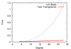
Figure 2: Generic dense bivariate systems.

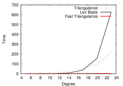
Figure 3: Highly non-equiprojectable bivariate systems.

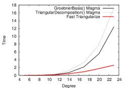
Figure 4: Highly non-equiprojectable bivariate systems.

Figure 2 compares FastTriangularize and (lexicographic) Groebner:-Basis in Maple on generic dense input systems. On the largest input example the former solver is about 20 times faster than the latter. Figure 3 compares FastTriangularize and (lexicographic) Groebner:-Basis on highly non-equiprojectable dense input systems; for these systems the number of equiprojectable components is about half the degree of the variety. At the total degree 23 our solver is approximately 100 times faster than Groebner:-Basis. Figure 4 compares FastTriangularize, GroebnerBasis in Magma and TriangularDecomposition in Magma on the same set of highly non-equiprojectable dense input systems. Once again our solver outperforms its competitors.

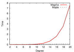
Figure 5: Generic dense trivariate systems.

For the solving of systems with two equations, we compare FastTriangularize (implementing in this case the algorithm described in Section 5.2) with GroebnerBasis in Magma. On Figure 5 these two solvers are simply referred as Magma and Maple. For this benchmark the input systems are generic dense trivariate systems.

Figures 6, 7 and 8 compare our fast regularity test algorithm (Algorithm 1) with the RegularChains library Regularize and its Magma counterpart. More precisely, in Magma, we first saturate the ideal generated by the input zerodimensional regular chain $T$ with the input polynomial $P$ using the Saturation command. Then the TriangularDecomposition command decomposes the output produced by the first step. The total degree of the input $i$-th polynomial in $T$ is $d_{i}$. For Figure 6 and Figure 7 the input $T$ and $P$ are random such that the intermediate computations do not split. In this “non-splitting” cases, our fast Regularize algorithm is significantly faster than the other commands.

For Figure 8 the input $T$ and $P$ are built such that many intermediate computations need to split. In this case, our fast Regularize algorithm is slightly slower than its Magma counterpart, but still much faster than the “generic” (non-modular and non-supported by modpn) Regularize command of the RegularChains library. The slow down w.r.t. the Magma code is due to the (large) overheads of the C - Maple interface, see [19] for details.

$d_{1}$	$d_{2}$	Regularize	Fast Regularize	Magma
2	2	0.052	0.016	0.000
4	6	0.236	0.016	0.010
6	10	0.760	0.016	0.010
8	14	1.968	0.020	0.050
10	18	4.420	0.052	0.090
12	22	8.784	0.072	0.220
14	26	15.989	0.144	0.500
16	30	27.497	0.208	0.990
18	34	44.594	0.368	1.890
20	38	69.876	0.776	3.660
22	42	107.154	0.656	6.600
24	46	156.373	1.036	10.460
26	50	220.653	2.172	17.110
28	54	309.271	1.640	25.900
30	58	434.343	2.008	42.600
32	62	574.923	4.156	57.000
34	66	746.818	6.456	104.780

Figure 6: 2-variable random dense case.

$d_{1}$	$d_{2}$	$d_{3}$	Regularize	Fast Regularize	Magma
2	2	3	0.240	0.008	0.000
3	4	6	1.196	0.020	0.020
4	6	9	4.424	0.032	0.030
5	8	12	12.956	0.148	0.200
6	10	15	33.614	0.360	0.710
7	12	18	82.393	1.108	2.920
8	14	21	168.910	2.204	8.250
9	16	24	332.036	14.764	23.160
10	18	27	$>$1000	21.853	61.560
11	20	30	$>$1000	57.203	132.240
12	22	33	$>$1000	102.830	284.420

Figure 7: 3-variable random dense case.

$d_{1}$	$d_{2}$	$d_{3}$	Regularize	Fast Regularize	V2.15-4	V2.14-8
2	2	3	0.184	0.028	0.000	0.000
3	4	6	0.972	0.060	0.000	0.010
4	6	9	3.212	0.092	$>$1000	0.030
5	8	12	8.228	0.208	$>$1000	0.150
6	10	15	21.461	0.888	807.850	0.370
7	12	18	51.751	3.836	$>$1000	1.790
8	14	21	106.722	9.604	$>$1000	2.890
9	16	24	207.752	39.590	$>$1000	10.950
10	18	27	388.356	72.548	$>$1000	19.180
11	20	30	703.123	138.924	$>$1000	56.850
12	22	33	$>$1000	295.374	$>$1000	76.340

Figure 8: 3-variable dense case with many splittings.

7 Conclusion

The concept of a regular GCD extends the usual notion of polynomial GCD from polynomial rings over fields to polynomial rings modulo saturated ideals of regular chains. Regular GCDs play a central role in triangular decomposition methods. Traditionally, regular GCDs are computed in a top-down manner, by adapting standard PRS techniques (Euclidean Algorithm, subresultant algorithms, …).

In this paper, we have examined the properties of regular GCDs of two polynomials w.r.t a regular chain. The theoretical results presented in Section 3 show that one can proceed in a bottom-up manner. This has three benefits described in Section 5. First, this algorithm is well-suited to employ modular methods and fast polynomial arithmetic. Secondly, we avoid the repetition of (potentially expensive) intermediate computations. Lastly, we avoid, as much as possible, computing modulo regular chains and use polynomial computations over the base field instead, while controlling expression swell. The experimental results reported in Section 6 illustrate the high efficiency of our algorithms.

8 Acknowledgement

The authors would like to thank our friend Changbo Chen, who pointed out that Lemma $3$ in an earlier version of this paper is incorrect.

References

- [1] M.F. Atiyah and L. G. Macdonald. Introduction to Commutative Algebra. Addison-Wesley, 1969.
- [2] F. Boulier, F. Lemaire, and M. Moreno Maza. Well known theorems on triangular systems and the D5 principle. In Proc. of Transgressive Computing 2006, Granada, Spain, 2006.
- [3] D.G. Cantor and E. Kaltofen. On fast multiplication of polynomials over arbitrary algebras. Acta Informatica, 28:693–701, 1991.
- [4] C. Chen, O. Golubitsky, F. Lemaire, M. Moreno Maza, and W. Pan. Comprehensive Triangular Decomposition, volume 4770 of LNCS, pages 73–101. Springer Verlag, 2007.
- [5] G.E. Collins. The calculation of multivariate polynomial resultants. Journal of the ACM, 18(4):515–532, 1971.
- [6] X. Dahan, M. Moreno Maza, É. Schost, and Y. Xie. On the complexity of the D5 principle. In Proc. of Transgressive Computing 2006, Granada, Spain, 2006.
- [7] J. Della Dora, C. Dicrescenzo, and D. Duval. About a new method for computing in algebraic number fields. In Proc. EUROCAL 85 Vol. 2, Springer-Verlag, 1985.
- [8] L. Ducos. Effectivité en théorie de Galois. Sous-résultants. PhD thesis, Université de Poitiers, 1997.
- [9] D. Duval. Questions Relatives au Calcul Formel avec des Nombres Algébriques. Université de Grenoble, 1987. Thèse d’État.
- [10] M’hammed El Kahoui. An elementary approach to subresultants theory. J. Symb. Comp., 35:281–292, 2003.
- [11] J. von zur Gathen and J. Gerhard. Modern Computer Algebra. Cambridge University Press, 1999.
- [12] T. Gómez Díaz. Quelques applications de l’évaluation dynamique. PhD thesis, Université de Limoges, 1994.
- [13] J. van der Hoeven. The Truncated Fourier Transform and applications. In ISSAC’04, pages 290–296. ACM, 2004.
- [14] M. Kalkbrener. A generalized euclidean algorithm for computing triangular representations of algebraic varieties. J. Symb. Comp., 15:143–167, 1993.
- [15] D. Lazard. A new method for solving algebraic systems of positive dimension. Discr. App. Math, 33:147–160, 1991.
- [16] D. Lazard. Solving zero-dimensional algebraic systems. J. Symb. Comp., 15:117–132, 1992.
- [17] F. Lemaire, M. Moreno Maza, W. Pan, and Y. Xie. When does equal ? In Proc. ISSAC’20008, pages 207–214. ACM Press, 2008.
- [18] F. Lemaire, M. Moreno Maza, and Y. Xie. The RegularChains library. In Ilias S. Kotsireas, editor, Maple Conference 2005, pages 355–368, 2005.
- [19] X. Li, M. Moreno Maza, R. Rasheed, and É. Schost. The modpn library: Bringing fast polynomial arithmetic into maple. In MICA’08, 2008.
- [20] X. Li, M. Moreno Maza, and É. Schost. Fast arithmetic for triangular sets: From theory to practice. In ISSAC’07, pages 269–276. ACM Press, 2007.
- [21] B. Mishra. Algorithmic Algebra. Springer, New York, 1993.
- [22] M. Moreno Maza. On triangular decompositions of algebraic varieties. Technical Report TR 4/99, NAG Ltd, Oxford, UK. Presented at the MEGA-2000 Conference, Bath, England.
- [23] M. Moreno Maza and R. Rioboo. Polynomial gcd computations over towers of algebraic extensions. In Proc. AAECC-11, pages 365–382. Springer, 1995.
- [24] V. Y. Pan. Simple multivariate polynomial multiplication. J. Symb. Comp., 18(3):183–186, 1994.
- [25] C. K. Yap. Fundamental Problems in Algorithmic Algebra. Princeton University Press, 1993.