A Study of Elliptical Last Stable Orbits About a Massive Kerr Black Hole

Abstract

The last stable orbit (LSO) of a compact object (CO) is an important boundary condition when performing numerical analysis of orbit evolution. Although the LSO is already well understood for the case where a test-particle is in an elliptical orbit around a Schwarzschild black hole (SBH) and for the case of a circular orbit about a Kerr black hole (KBH) of normalised spin, ${\tilde{S}}$ (${\left|{\mathbf{J}}\right|}/M^{2}$, where ${\mathbf{J}}$ is the spin angular momentum of the KBH); it is worthwhile to extend our knowledge to include elliptical orbits about a KBH. This extension helps to lay the foundation for a better understanding of gravitational wave (GW) emission.

The mathematical developments described in this work sprang from the use of an effective potential (${\tilde{V}}$) derived from the Kerr metric, which encapsulates the Lense-Thirring precession. That allowed us to develop a new form of analytical expression to calculate the LSO Radius for circular orbits (${R_{LSO}}$) of arbitrary KBH spin. We were then able to construct a numerical method to calculate the latus rectum (${\tilde{l}}_{LSO}$) for an elliptical LSO.

Formulae for ${\tilde{E}}^{2}$ (square of normalised orbital energy) and ${\tilde{L}}^{2}$ (square of normalised orbital angular momentum) in terms of eccentricity, ${\varepsilon}$, and latus rectum, ${\tilde{l}}$, were previously developed by others for elliptical orbits around an SBH and then extended to the KBH case; we used these results to generalise our analytical ${{\tilde{l}}_{LSO}}$ equations to elliptical orbits. LSO data calculated from our analytical equations and numerical procedures, and those previously published, are then compared and found to be in excellent agreement.

*Department of Physics and Astronomy, #Department of Applied Mathematics, University of Western Ontario, London, Ontario

pkomorow@uwo.ca, valluri@uwo.ca, houde@astro.uwo.ca

04.20.-q, 95.30.Sf, 95.75.Pq

1 Introduction

One of the most important goals in experimental gravitation today is the detection of gravitational wave (GW) radiation [1, 2, 3]. To achieve this goal, considerable effort has been made to improve the theoretical understanding of the evolution of compact object (CO) orbits in extreme black hole systems [4, 5, 6, 7, 8, 9]. In this paper, we assume a point-like test-particle since the ratio of CO mass to the mass of the massive black hole (MBH) will be small (i.e. $\leq{10}^{-5}$ [10]); and the effect of the CO mass upon the post Newtonian (PN) equations that we will use in our subsequent modelling of the CO orbits is negligible [11, 2, 4]. In this paper, we shall then assume the behaviour of the CO to be closely approximated by that of a test-particle. If reference is made to the orbital evolution of a true CO, as described by the PN evolution equations, then we will use the term, CO. The treatment of CO orbital evolution we will present in a forthcoming paper will be based on the work of [4, 5, 12, 11, 6, 7, 8, 13] in which PN equations for a rotating MBH, also called a Kerr black hole (KBH), are considered.

The objective of this study is to lay the foundation for our subsequent work that will include the numerical calculation of the GW energy emission by extreme KBH systems where the CO is in an elliptical orbit in the equatorial plane of the KBH. The most basic quadrupole model [4, 5] admitted solutions in closed form [5, 14]; but because the more comprehensive evolution equations now used are too complicated to admit an analytical solution, numerical integration of orbital parameters is required [8]. Therefore the last stable orbit (LSO) becomes an important boundary condition. Such an analysis requires an understanding of how ${\tilde{V}}$ depends on ${\tilde{L}}$ and on the inclination of the CO orbit. To undertake future work for inclined orbits it is important to know the minimum physically meaningful value of ${\tilde{L}}$.

Previous research has demonstrated how the effective potential (${\tilde{V}}$) of a test-particle in an equatorial orbit around a Schwarzschild black hole (SBH) [15, 16, 17] can be calculated from the Schwarzschild metric and used to determine the latus rectum of the LSO (${{\tilde{l}}_{LSO}}$). A treatment of ${\tilde{V}}$ for a KBH system, where the test-particle follows a circular LSO (section 12.7 of [18]) yields an analytical expression for the value ${R_{LSO}}$ in terms of normalised spin, ${\tilde{S}}$, (equation 12.7.24 in [18], [19]) (${\tilde{S}}={\left|{\mathbf{s}}\right|}/M$ where ${\mathbf{s}}={\mathbf{J}}/M$ and ${\mathbf{J}}$ represents the spin angular momentum of the KBH). Such treatment of ${\tilde{V}}$ also gives rise to expressions (equations 12.7.17 and 12.7.18 in [18]) for the orbital energy, ${\tilde{E}}$, and orbital angular momentum, ${\tilde{L}}$. In [16] the energy and orbital angular momentum equations were also derived for an SBH system with the test-particle in an elliptical orbit. In the significant work by Glampedakis and Kennefick [2], their treatment of ${\tilde{E}}$ and the quantity, $\left({\tilde{L}}-{\tilde{S}}{\tilde{E}}\right)$, enabled us to derive generalised ${R_{LSO}}$ formulae for elliptical orbits. Analytical expressions have a clear usefulness in the development of new theoretical concepts and numerical methods [10, 20].

The Lense-Thirring effect, an apodeictic [21] prediction of general relativity, is the means by which the rotation of the KBH imparts important changes on the test-particle orbit [22, 23, 21, 24] that are distinct from those associated with the SBH. The swirling of spacetime in the vicinity of the KBH applies a torsion to the orbiting test-particle; therefore, the orbit evolution will be altered, thus causing changes in the point at which the test-particle reaches its LSO. We shall develop an analytical and numerical methodology to calculate the LSO of a test-particle in elliptical orbit about a KBH. Numerical estimates of the latus rectum of the elliptical LSO orbits with respect to KBH spin are available in the literature (Table I in [2], based upon the work of Schmidt [25], and Table I in [10]); and they will provide a means to validate our results.

In section 2.1, the Kerr metric is introduced and used in section 2.2 as the basis of developing some essential analytical formulae to calculate the orbital angular momentum of test-particles in circular paths around a KBH (section 2.3). A formula for ${R}_{LSO}$ (prograde and retrograde) is then developed analytically; and the general formula for the ${{\tilde{l}}_{LSO}}$ of elliptical orbits is also presented. In section 2.4 the development and demonstration of a numerical algorithm to determine the latus rectum and eccentricity of test-particles of higher orbital angular momentum then follows. The results of this analysis (section 2.5), as well as results obtained from the general analytical formulae for LSO latus rectum, are compared with results obtained from the literature. In section 3 we shall draw conclusions.

2 Understanding the Last Stable Orbit About a Rotating Massive Black Hole

2.1 Kerr Metric

The Kerr metric (See equation 13.12 in [26]) represents the solution to the Einstein Field Equations in the case where the MBH possesses spin angular momentum,

$$g_{\alpha\beta}\Biggr{|}_{\mathit{Kerr}}=\left[\begin{array}[]{cccc}-{\frac{\Delta-{M^{2}}{\tilde{S}}^{2}\sin^{2}\left(\theta\right)}{{\rho}^{2}}}&0&0&-2{M}{\frac{{M^{2}}\tilde{S}R\sin^{2}\left(\theta\right)}{{\rho}^{2}}}\\ \vskip 6.0pt plus 2.0pt minus 2.0pt\cr 0&{\frac{{\rho}^{2}}{\Delta}}&0&0\\ \vskip 6.0pt plus 2.0pt minus 2.0pt\cr 0&0&{\rho}^{2}&0\\ \vskip 6.0pt plus 2.0pt minus 2.0pt\cr-2{M}{\frac{{M^{2}}\tilde{S}R\sin^{2}\left(\theta\right)}{{\rho}^{2}}}&0&0&{\frac{{M^{4}}\left({R}^{2}+{\tilde{S}}^{2}\right)^{2}-{M^{2}}{\tilde{S}}^{2}\Delta\,\sin^{2}\left(\theta\right)}{{\rho}^{2}}\sin^{2}\left(\theta\right)}\end{array}\right],$$ (1)

where $\rho={M}\sqrt{{R}^{2}+\cos^{2}\left(\theta\right){\tilde{S}}^{2}}$ and $\Delta={M^{2}}\left({R}^{2}-2\,R+{\tilde{S}}^{2}\right)$; in which the factors, $R=r/M$ and $\tilde{S}={\left|\mathbf{J}\right|}/M^{2}$, are used to express the metric in dimensionless terms. The symmetric off-diagonal elements, $-2{M^{3}}\tilde{S}R\sin^{2}\left(\theta\right)/{\rho}^{2}$, correspond to the Lense-Thirring precession that arises from the spin of a central KBH of mass, ${M}$. Observe that when, $\tilde{S}=0$, the Kerr metric equals the Schwarzschild Metric.

Although the Schwarzschild Metric is expressed in spherical coordinates, when the central black hole rotates it is appropriate to use the Kerr metric expressed in Boyer-Lindquist (BL) coordinates. The conversion of the BL coordinate system variables to Cartesian coordinate variables is represented by these equations (see equation 11.4.7 in [27] and see also [28]) :

$$x = \sqrt{{R}_{BL}^{2}+{\tilde{S}}^{2}}\sin\left(\theta\right)\cos\left(\phi-f\right),$$

$$y = \sqrt{{R}_{BL}^{2}+{\tilde{S}}^{2}}\sin\left(\theta\right)\sin\left(\phi-f\right),$$

$$z = {R}_{BL}\cos\left(\theta\right),$$ (2)

where

$${f}=\pm{\arctan\left({\nicefrac{{\tilde{S}}}{{R_{BL}}}}\right)}.$$ (3)

Because $0\leq{\tilde{S}}<1.0$, a prograde or retrograde orbit is represented by the respective use of a plus or minus sign in equation (3). The BL coordinate system will be used throughout this treatment. The conversion of LSO radius from BL to spherical coordinates is required whenever one performs a simulation of the evolution equations reported in [29, 7, 30, 31, 8]. This conversion is uncomplicated in the current application (in which the angle, ${\iota}$, between the orbital angular momentum vector and the spin axis of the KBH is zero), and proceeds by adding the squares of $x,y,$ and $z$ as shown in equation (2) to obtain,

$${R}_{Spherical}^{2}={x}^{2}+{y}^{2}+{z}^{2}.$$ (4)

By substituting the relationships in equation (2) into equation (4) , one obtains the mathematical relationship,

$$R_{Spherical}^{2}=R_{BL}^{2}+\tilde{S}^{2}{\sin^{2}\left(\theta\right)}.$$ (5)

Recall that ${\tilde{S}}$ is the normalised spin of the KBH and ${\theta}$ is the polar angle of the test-particle in its orbit. In this study, we work with orbits that are exclusively in the equatorial plane of the KBH. Therefore one sets ${\theta}={\frac{\pi}{2}}$ to obtain

$$R_{Spherical}^{2}=R_{BL}^{2}+\tilde{S}^{2}.$$ (6)

Such a relationship is required for transforming LSO radii (BL coordinates) into the spherical coordinate system.

2.2 Effective Potential

We shall develop a formulation of the effective potential of a test-particle in orbit about a KBH. By so doing, the location of the LSO can be estimated. In the following equations and calculations the radius, ${R}$, is represented in BL coordinates. For simplicity of notation, the BL subscript will be suppressed (except in Section 2.5.2).

The four-momentum can be expressed as:

$$P_{\gamma} = \biggl{[}-E,\>m\frac{{\rho}^{2}}{\Delta}\left({\it\frac{dR}{d\tau}}\right),\>0,\>{m}{M}\tilde{L}\biggr{]}$$ (7)

for a particle of mass ${m}$ and,

$$P_{\gamma} = \biggl{[}-E,\>\frac{{\rho}^{2}}{\Delta}\left({\it\frac{dR}{d\lambda}}\right),\>0,\>L\biggr{]},$$ (8)

for zero mass, where $E$ is the energy of the orbital element and $\tilde{L}$ is the orbital angular momentum of the particle in orbit normalised with respect to its mass, $m$, and the KBH mass, ${M}$. The $\left(dR/d\tau\right)$ is the derivative of the radial component of the compact object with respect to the proper time, $\tau$. For the zero-mass particle (which has no rest mass), ${L}$ is its total linear momentum (vis. ${L}={E}_{photon}/{c}$). The factor, $dR/d\lambda$, is the derivative of the radial component of the zero-mass particle with respect to an affine parameter, $\lambda$, which is used in place of proper time, $\tau$, since a zero-mass particle always follows a null path.

The invariant quantity of mass-energy can be calculated for each case of a test-particle of infinitesimal mass

$$\vec{P}\cdot\vec{P} = \left.P_{\gamma}P_{\delta}g^{\delta\gamma}\right|_{Kerr}=-{m}^{2},$$ (9)

and a zero-mass particle

$$\vec{P}\cdot\vec{P} = \left.P_{\gamma}P_{\delta}g^{\delta\gamma}\right|_{Kerr}=0.$$ (10)

In that respect, the expected behaviour of a test mass will differ from that of a zero-mass orbital element. From these equations, the effective potential can be calculated by making a few assumptions about the path taken by the orbiting zero-mass particle. The inverse Kerr metric ($g^{\delta\gamma}$) is shown in Appendix A (equations (77) and (83)).

2.2.1 Test Particle.

We restrict our work to the case of a test particle of mass, $m$, in orbit about a KBH with ${\theta}={\frac{\pi}{2}}$. By evaluating $\vec{P}\cdot\vec{P}$ (see equation (9)) using the test mass four-momentum (see equation (7)) one obtains,

$$\vec{P}\cdot\vec{P} =- \Biggl{(}{R}^{4}{E}^{2}-{R}^{4}{m}^{2}\left(\frac{dR}{d\tau}\right)^{2}-{R}^{2}{m}^{2}{\tilde{L}}^{2}+{R}^{2}{E}^{2}{\tilde{S}}^{2}$$ (11)

$$+2\,R{E}^{2}{\tilde{S}}^{2}+2\,R{m}^{2}{\tilde{L}}^{2}+4\,RE\tilde{S}m\tilde{L}\Biggr{)}$$

$$\times \left({R}^{4}-2\,{R}^{3}+{R}^{2}{\tilde{S}}^{2}\right)^{-1}$$

$$= -m^{2}.$$

To develop a relationship between the effective potential and the orbital parameters several sequential steps must be followed. First, all terms in equation (11) are collected and equated to zero, and then divided by $m^{2}$ and the $\left({dR}/{d\tau}\right)^{2}$ terms are collected on the right hand side of the equation. Noting that ${E/m}={\tilde{E}}$ represents the specific energy content of the orbiting test-particle, one then obtains,

$$\left({R^{2}{\tilde{S}}^{2}+2R{\tilde{S}}^{2}+R^{4}}\right)\tilde{E}^{2}-\left(4R{\tilde{S}}\tilde{L}\right)\tilde{E}$$ (12)

$$- \left(\tilde{L}^{2}R^{2}-2\tilde{L}^{2}R+R^{2}\left({R^{2}-2R+{\tilde{S}}^{2}}\right)\right)$$

$$= R^{4}\left({\frac{{dR}}{{d\tau}}}\right)^{2}$$

At the points of closest (pericentre) and farthest (apocentre) approach the derivative of ${R}$ with respect to $\tau$ is zero. By performing that simplification, one obtains a quadratic equation in $\tilde{E}$, i.e.

$$- \left({R^{2}{\tilde{S}}^{2}+2R{\tilde{S}}^{2}+R^{4}}\right)\tilde{E}^{2}+\left(4R{\tilde{S}}\tilde{L}\right)\tilde{E}$$ (13)

$$+ \left(\tilde{L}^{2}R^{2}-2\tilde{L}^{2}R+R^{2}\left({R^{2}-2R+{\tilde{S}}^{2}}\right)\right)$$

$$= 0.$$

The factored form of equation (13) corresponds to the following equation [17]:

$$\left(\tilde{E}-{\tilde{V}}_{+}\right)\left(\tilde{E}-{\tilde{V}}_{-}\right) = 0.$$ (14)

Therefore two solutions for the effective potential can be calculated:

$$\tilde{V}_{\pm} = \frac{-b\mp\sqrt{b^{2}-4ac}}{2a}$$ (15)

$$a = -\left({R}^{4}+{R}^{2}{\tilde{S}}^{2}+2\,{\tilde{S}}^{2}R\right)$$

$$b = 4\,R\tilde{S}\tilde{L}$$

$$c = \left(L^{2}R^{2}-2L^{2}R+R^{2}\left({R^{2}-2R+{\tilde{S}}^{2}}\right)\right).$$

For the SBH (i.e. ${\tilde{S}}=0$), the value of ${\tilde{V}_{\pm}}^{2}$ (from equation (15)) becomes:

$${\tilde{V}_{\pm}}^{2} = \frac{\left(R-2\right)\left({R}^{2}+{\tilde{L}}^{2}\right)}{{R}^{3}},$$ (16)

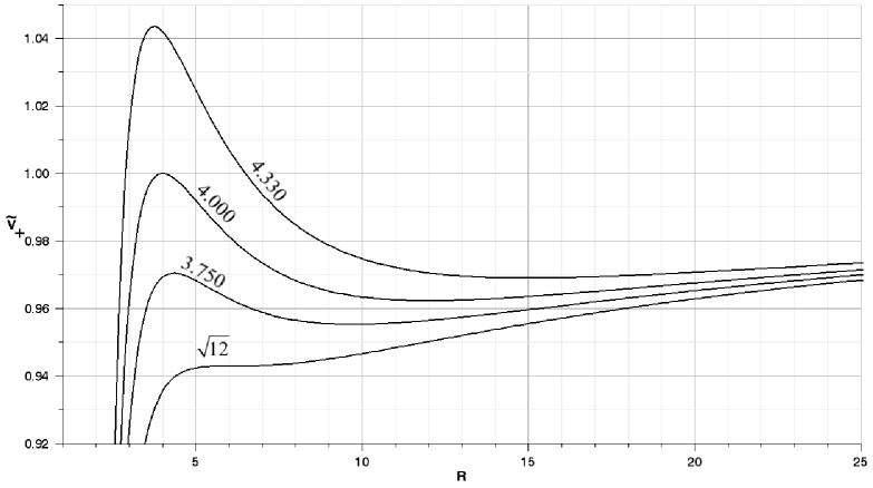
Figure 1: Effective Potentials for various values of ${\tilde{L}}$ where ${\tilde{S}}=0$.

which depends only on the values of $R$ and $\tilde{L}$, as expected (as shown in Figure 1).

The effective potential contains important information. In the case of the SBH, the relationship between ${V}_{\pm}$ and ${R}$ describes the test-particle orbit and leads us to a calculation of the values of $\tilde{L}$ and ${R}$ at which the test-particle can no longer sustain a stable orbit. The LSO is an important characteristic of the binary system that is identified as the point at which the ${\tilde{V}}_{+}$ curve (Figure 1) has a slope of zero and the second derivative with respect to ${R}$ is not positive. The effective potential, ${\tilde{V}}_{-}$, corresponds to particles and photons for which their orbital angular momentum has an opposite sense to the KBH spin (section 11.3 in [17]). The mathematical treatment of ${\tilde{V}}_{+}$ presented in the sections that follow preserves its prograde and retrograde properties; indeed, we have found that the use of ${\tilde{V}}_{-}$ in the calculations that follow yield the same results.

2.3 Last Stable Orbit (LSO) for a CO in the Equatorial Plane of the Kerr Black Hole

The equations for the radius of a circular or elliptical LSO can be calculated through a mathematical treatment of the following two equations:

$$\frac{d{\tilde{V}}_{+}}{{dR}} = 0$$ (17)

and

$$\frac{d^{2}{\tilde{V}}_{+}}{{dR}^{2}} \leq 0,$$ (18)

where the point of inflection (which corresponds to a circular LSO) can be found by evaluating the intersection points of the equations (17) and (18).

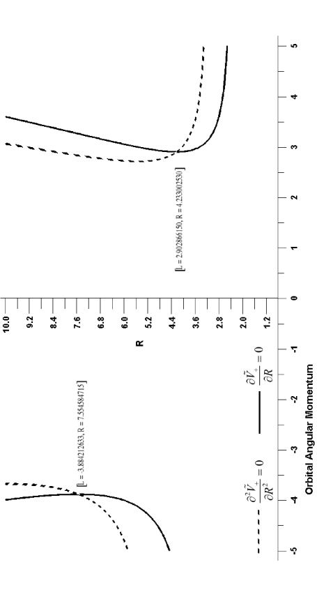
Figure 2: A plot of ${R}_{LSO}$ vs. ${\tilde{L}}$ for the first and second derivatives of ${\tilde{V}}$ with respect to ${R}$.

The loci of these two equations is depicted in the $\left({R,\tilde{L}}\right)$ plane for a KBH with a spin value of ${\tilde{S}}=0.5$ (see Figure 2). Their intersection points (derived numerically with Maple 11), $\left[\begin{array}[]{cc}{R}=7.554584715,&{\tilde{L}}=-3.884212633\end{array}\right]$ and $\left[\begin{array}[]{cc}{R}=4.233002530,&{\tilde{L}}=2.902866150\end{array}\right]$, correspond to the radial position of the LSO, $R$, of a test-particle with an orbital angular momentum of ${\tilde{L}}$. These points differ from $\left[\begin{array}[]{cc}{R}=6.0,&{\tilde{L}}=\pm\sqrt{12}\end{array}\right]$, which is the solution for an SBH. The existence of an intersection point on the graphical plot notwithstanding (see Figure 2), on frequent occasions, no result was returned by Maple. On other occasions a correct value of ${R}$ was returned, while the value calculated for ${\tilde{L}}$ deviated by at least a factor of two from the graphical result. Such inconsistent behaviour was attributed to the great complexity of the expressions being treated and the associated floating point round off error; therefore, an analytic method was sought.

2.3.1 Orbital Angular Momentum.

The derivative of ${\tilde{V}_{+}}$, equated to zero, can be used to determine an analytical expression for $\tilde{L}^{2}$ in terms of $R$ and ${\tilde{S}}$ for circular or elliptical orbits. From equations (15) and (17) one obtains,

$$\frac{d\tilde{V}_{+}}{dR} = \Biggl{(}-3\,{S}^{2}{R}^{4}{L}^{2}+6\,{S}^{2}{R}^{3}{L}^{2}-2\,{R}^{2}{S}^{4}{L}^{2}$$ (19)

$$+{R}^{5}{L}^{2}{S}^{2}+2\,{S}^{2}{R}^{5}-3\,{R}^{6}{S}^{2}-3\,{R}^{6}{L}^{2}$$

$$-3\,{S}^{4}{R}^{4}-{S}^{6}{R}^{2}-2\,R{S}^{6}+8\,{S}^{4}{R}^{2}-{R}^{8}+{R}^{7}{L}^{2}$$

$$+\left(6\,{R}^{2}SL+2\,{S}^{3}L\right)\sqrt{{R}^{3}\left({R}^{2}-2\,R+{S}^{2}\right)\left({R}^{3}+{L}^{2}R+{S}^{2}R+2\,{S}^{2}\right)}\Biggr{)}$$

$$\div \Biggl{(}\sqrt{{R}^{3}\left({R}^{2}-2\,R+{S}^{2}\right)\left({R}^{3}+{L}^{2}R+{S}^{2}R+2\,{S}^{2}\right)}$$

$$\left({R}^{3}+{S}^{2}R+2\,{S}^{2}\right)^{2}\Biggr{)}$$

$$= 0.$$

The denominator of equation (19) can be disregarded because the quotient is equated to zero; it is also required that the roots of the factors present in the denominator lie outside the range of physically attainable ${R}$ values. To be specific, the roots of $\left({R}^{2}-2\,R+{\tilde{S}}^{2}\right)$ correspond to the event horizon for massless particles, those of ${R}^{3}$ are zero and beyond the LSO, and the roots of $\left({R}^{3}+{\tilde{L}}^{2}R+{\tilde{S}}^{2}R+2\,{\tilde{S}}^{2}\right)$ and $\left({R}^{3}+{\tilde{S}}^{2}R+2\,{\tilde{S}}^{2}\right)$ are complex and thus also physically unattainable for real values of ${R}$.

The simplified power series is thus derived from the numerator of equation (19) after eliminating the square root,

$${R}^{3}\left(9\,R-6\,{R}^{2}+{R}^{3}-4\,{\tilde{S}}^{2}\right){\tilde{L}}^{4}$$

$$-2\,{R}^{2}\left(-3\,{R}^{4}+{R}^{5}-12\,{\tilde{S}}^{2}R+6\,{R}^{2}{\tilde{S}}^{2}+2\,{R}^{3}{\tilde{S}}^{2}+5\,{\tilde{S}}^{4}+{\tilde{S}}^{4}R\right){\tilde{L}}^{2}$$

$$+\left({R}^{4}+2\,{R}^{2}{\tilde{S}}^{2}-4\,{\tilde{S}}^{2}R+{\tilde{S}}^{4}\right)^{2}$$

$$=0.$$ (20)

Therefore $\tilde{L}^{2}$ can be obtained directly by using the quadratic formula,

$$\tilde{L}^{2}=\frac{-b\pm\sqrt{b^{2}-4ac}}{2a},$$ (21)

where we have redefined:

$${a} = {R}^{3}\left(9\,R-6\,{R}^{2}+{R}^{3}-4\,{\tilde{S}}^{2}\right)$$

$${b} = -2\,{R}^{2}\left(-3\,{R}^{4}+{R}^{5}-12\,{\tilde{S}}^{2}R+6\,{R}^{2}{\tilde{S}}^{2}+2\,{R}^{3}{\tilde{S}}^{2}+5\,{\tilde{S}}^{4}+{\tilde{S}}^{4}R\right)$$

$${c} = \left({R}^{4}+2\,{R}^{2}{\tilde{S}}^{2}-4\,{\tilde{S}}^{2}R+{\tilde{S}}^{4}\right)^{2}.$$

Two solutions are found that correspond to the orbital angular momenta of a test-particle in a prograde orbit,

$${\tilde{L}}_{Pro}^{2} = \left(-3\,{R}^{6}+{R}^{7}-12\,{R}^{3}{\tilde{S}}^{2}+6\,{R}^{4}{\tilde{S}}^{2}\right.$$ (22)

$$+2\,{R}^{5}{\tilde{S}}^{2}+5\,{\tilde{S}}^{4}{R}^{2}+{\tilde{S}}^{4}{R}^{3}$$

$$\left.-2\,{\tilde{S}}\left(3\,{R}^{2}+{\tilde{S}}^{2}\right)\left({R}^{2}-2\,R+{\tilde{S}}^{2}\right)\sqrt{{R}^{3}}\right)$$

$$\left({R}^{3}\left(9\,R-6\,{R}^{2}+{R}^{3}-4\,{\tilde{S}}^{2}\right)\right)^{-1},$$

and in a retrograde orbit,

$${\tilde{L}}_{Ret}^{2} = \left(-3\,{R}^{6}+{R}^{7}-12\,{R}^{3}{\tilde{S}}^{2}+6\,{R}^{4}{\tilde{S}}^{2}\right.$$ (23)

$$+2\,{R}^{5}{\tilde{S}}^{2}+5\,{\tilde{S}}^{4}{R}^{2}+{\tilde{S}}^{4}{R}^{3}$$

$$\left.+2\,{\tilde{S}}\left(3\,{R}^{2}+{\tilde{S}}^{2}\right)\left({R}^{2}-2\,R+{\tilde{S}}^{2}\right)\sqrt{{R}^{3}}\right)$$

$$\left({R}^{3}\left(9\,R-6\,{R}^{2}+{R}^{3}-4\,{\tilde{S}}^{2}\right)\right)^{-1}.$$

An analytical expression for ${\tilde{L}}^{2}$ with respect to ${R}$ and ${\tilde{S}}$ has been derived. But one must consider that the formula is limited to providing a value of ${\tilde{L}}^{2}$ that corresponds to a test-particle in its LSO (BL coordinates) about a KBH of spin ${\tilde{S}}$. These formulae (equations (22) and (23)) do not provide a relationship between ${R}$ and ${\tilde{L}}^{2}$ for a general orbit.

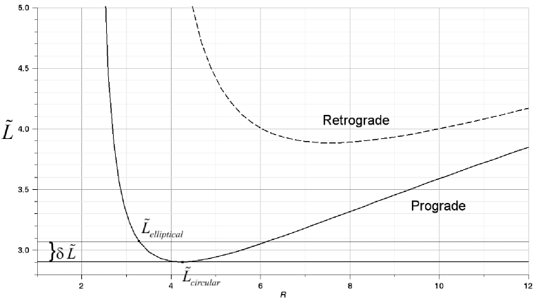
Figure 3: The relationship between the orbital angular momentum, ${\tilde{L}}$, and radius ${R}$ for a prograde and retrograde orbit.

Consider an example where ${\tilde{S}}=0.5$. The relationship between the value of ${\tilde{L}}$ and the radius $R\in[1.0,\>6.0]$ is plotted in Figure 3. One observes a power series for which the values of ${R}$ and ${\tilde{L}}$ for a circular orbit (at the point of inflection) occur at the local minimum. Therefore it is possible to derive an expression for the radius of the LSO, ${R}_{LSO}$, at that point of inflection for an arbitrary spin, ${\tilde{S}}$, where $0\leq{\tilde{S}}<1$.

2.3.2 Circular LSO Radius.

The calculation of such an analytical relationship proceeds as follows. The derivative of ${\tilde{L}}^{2}$ with respect to ${R}$ is set equal to zero. From equation (21) we obtain:

$$\frac{d\left({\tilde{L}}^{2}\right)}{d{R}} = \Biggl{[}{\tilde{S}}\sqrt{{R}}/{R}\left(3R^{7}-45R^{5}+20{\tilde{S}}^{2}R^{5}+54R^{4}-26{\tilde{S}}^{2}R^{4}\right.$$ (24)

$$+9{\tilde{S}}^{4}R^{3}+24{\tilde{S}}^{2}R^{3}-26{\tilde{S}}^{4}R^{2}-54{\tilde{S}}^{2}R^{2}+53{\tilde{S}}^{4}R-12{\tilde{S}}^{6}\Bigr{)}$$

$$\pm \Bigl{(}R^{8}-2R^{6}{\tilde{S}}^{2}-3R^{4}{\tilde{S}}^{4}-12R^{7}-28{\tilde{S}}^{2}R^{5}-24{\tilde{S}}^{4}R^{3}$$

$$+45R^{6}+126{\tilde{S}}^{2}R^{4}+57{\tilde{S}}^{4}R^{2}+20{\tilde{S}}^{6}$$

$$-54R^{5}-144{\tilde{S}}^{2}R^{3}-90{\tilde{S}}^{4}R+108{\tilde{S}}^{2}R^{2}\Bigr{)}\Biggr{]}$$

$$\times \left[{R^{2}\left({-R^{3}+4{\tilde{S}}^{2}+6R^{2}-9R}\right)^{2}}\right]^{-1}=0.$$

Where the plus sign corresponds to a prograde orbit and the minus sign corresponds to a retrograde orbit. The denominator contains a factor (i.e. $\left({-R^{3}+4{\tilde{S}}^{2}+6R^{2}-9R}\right)$) with roots that correspond to the event horizon and a factor $R^{2}$ with roots equal to zero, which lie beyond the event horizon and are thus unattainable.

Table 1: A summary of the factors found in equation (25) for ${\tilde{S}}=0.0,\>0.5,$ and $1.0$.

Factor	${\tilde{S}}=0.0$	${\tilde{S}}=0.5$	${\tilde{S}}=1.0$	Comments
$\left({\tilde{S}}^{2}-{R}^{3}\right)$	$\left\{\begin{array}[]{c}0\\ 0\\ 0\end{array}\right\}$	$\left\{\begin{array}[]{c}0.629961\\ -0.315\left(1\pm i\,\sqrt{3}\right)\end{array}\right\}$	$\left\{\begin{array}[]{c}1.0\\ -0.5\left(1\pm i\,\sqrt{3}\right)\end{array}\right\}$
$\begin{array}[]{c}\left(9\,{\tilde{S}}^{4}-28\,{\tilde{S}}^{2}R-6\,{\tilde{S}}^{2}{R}^{2}\right.\\ \left.+36\,{R}^{2}-12\,{R}^{3}+{R}^{4}\right)\end{array}$	$\left\{\begin{array}[]{c}0\\ 0\\ 6\\ 6\end{array}\right\}$	$\left\{\begin{array}[]{c}0.10620\ldots\pm i\,0.079436\ldots\\ 4.233002530\\ 7.554584715\end{array}\right\}$	$\left\{\begin{array}[]{c}1\\ 1\\ 1\\ 9\end{array}\right\}$	Corresponds to radius of LSO for test mass particles.
$\left({\tilde{S}}^{4}+2\,{\tilde{S}}^{2}{R}^{2}-4\,{\tilde{S}}^{2}R+{R}^{4}\right)$	$\left\{\begin{array}[]{c}0\\ 0\\ 0\\ 0\end{array}\right\}$	$\left\{\begin{array}[]{c}0.06460427\ldots\\ 0.80423269\ldots\\ -0.4344\pm i\,1.00708\ldots\end{array}\right\}$	$\left\{\begin{array}[]{c}0.295598\ldots\\ 1\\ -0.64780\pm i\,1.7214\ldots\end{array}\right\}$
$\left({R}^{3}-4\,{\tilde{S}}^{2}-6\,{R}^{2}+9\,R\right)$	$\left\{\begin{array}[]{c}0\\ 3\\ 3\end{array}\right\}$	$\left\{\begin{array}[]{c}0.120615\ldots\\ 2.347300\ldots\\ 3.532090\ldots\end{array}\right\}$	$\left\{\begin{array}[]{c}1\\ 1\\ 4\end{array}\right\}$	Corresponds to radius of LSO for massless particles (e.g. photons or gravitons).

The simplification of the equation by taking only the numerator and eliminating the square root, can proceed to yield the following result:

$${R}^{3}\left({\tilde{S}}^{2}-{R}^{3}\right)\left(9\,{\tilde{S}}^{4}-28\,{\tilde{S}}^{2}R-6\,{\tilde{S}}^{2}{R}^{2}+36\,{R}^{2}-12\,{R}^{3}+{R}^{4}\right)$$ (25)

$$\times \left({\tilde{S}}^{4}+2\,{\tilde{S}}^{2}{R}^{2}-4\,{\tilde{S}}^{2}R+{R}^{4}\right)\left({R}^{3}-4\,{\tilde{S}}^{2}-6\,{R}^{2}+9\,R\right)^{2}$$

$$= 0.$$

Fortunately, the polynomial that expresses the relationship between ${\tilde{S}}$ and ${R}_{LSO}$, is already simplified into a product of some binomials, trinomials, and quartics (see Table 1). Each one can be assessed by considering the examples of an SBH with no spin (${\tilde{S}}=0.0$) and a KBH with ${\tilde{S}}=0.5$. For the former case, the solution, $\left[\begin{array}[]{cc}{R}=6.0,&{\tilde{L}}=\sqrt{12}\end{array}\right]$, is known; for the second case, it has been calculated numerically, $\left[\begin{array}[]{cc}{R}=4.233002530,&{\tilde{L}}=2.902866150\end{array}\right]$. These cases help one to identify the relevant factor. It is interesting to observe that some of the radii in Table 1 have complex values.

The factor that yields the values of the LSO radii (one for each of the possible prograde and retrograde orbits of the CO) is:

$$\left(9\,{\tilde{S}}^{4}-28\,{\tilde{S}}^{2}R-6\,{\tilde{S}}^{2}{R}^{2}+36\,{R}^{2}-12\,{R}^{3}+{R}^{4}\right)=0.$$ (26)

This quartic equation (26) can be converted to a companion matrix which is solved for its eigenvalues to yield the analytical solutions for ${R}_{LSO}$ for the prograde and retrograde orbits (see Appendix B). These solutions are:

$${R}_{pro} = 3+\sqrt{{Z}}-\sqrt{\frac{16{\tilde{S}}^{2}}{\sqrt{{Z}}}-{Z}+3\left(3+{\tilde{S}}^{2}\right)}$$ (27)

and

$${R}_{ret} = 3+\sqrt{{Z}}+\sqrt{\frac{16{\tilde{S}}^{2}}{\sqrt{{Z}}}-{Z}+3\left(3+{\tilde{S}}^{2}\right)}$$ (28)

where:

$$Z = 3+{\tilde{S}}^{2}+(3+\tilde{S})\left((1+\tilde{S})(1-\tilde{S})^{2}\right)^{\frac{1}{3}}$$

$$+(3-\tilde{S})\left((1-\tilde{S})(1+\tilde{S})^{2}\right)^{\frac{1}{3}}.$$

Although formulae that are analytically the same as ours have already been developed by Bardeen et al. [19], our formulae were derived by independent means and are simpler. The numerical results of each equation differ insignificantly over the physically valid range of $0\leq{\tilde{S}}<1.0$. And our formulae are more robust with respect to round-off error when evaluated numerically, and they are roborant of the pre-existing calculations.

2.3.3 Orbital Energy and Angular Momentum at the LSO.

One can derive new formulae for the test-particle orbital energy, ${\tilde{E}}$, and angular momentum, ${\tilde{L}}$, in terms of parameters ${\tilde{S}}$, ${\varepsilon}$, and latus rectum, ${\tilde{l}}$, by using equation (15) as a starting point. We know that,

$${\tilde{V}}_{+}={\tilde{E}},$$ (29)

$\Rightarrow$

$${\tilde{E}} = \Biggl{[}{2R{\tilde{S}}\tilde{L}+}$$ (30)

$$\sqrt{R\left({R^{2}-2R+{\tilde{S}}^{2}}\right)\left({R^{5}+R^{3}\tilde{L}^{2}+R^{3}{\tilde{S}}^{2}+2R^{2}{\tilde{S}}^{2}}\right)}\Biggr{]}$$

$$\Biggl{[}{R\left({R^{3}+{\tilde{S}}^{2}R+2{\tilde{S}}^{2}}\right)}\Biggr{]}^{-1}$$

when the test-particle is in its LSO. Although the roots in ${R}$ are readily found by Maple, they are inordinately long and not useful. A more effective derivation method, similar to the one used in [2], shall be outlined.

By manipulating the formula in equation (30) we obtain:

$${R}^{3}-\left(\frac{2}{1-{\tilde{E}}^{2}}\right){R}^{2}+\left(\frac{{\tilde{L}}^{2}+{\tilde{S}}^{2}-{\tilde{E}}^{2}{\tilde{S}}^{2}}{1-{\tilde{E}}^{2}}\right){R}$$

$$-\left(\frac{2\left({\tilde{L-}\tilde{E}\tilde{S}}\right)^{2}}{1-{\tilde{E}}^{2}}\right) = 0$$ (31)

from which we can obtain the expressions for the sum and the product of the roots in ${R}$ directly from the coefficients of the polynomial, vis.

$$\left(R-r_{1}\right)\left(R-r_{2}\right)\left(R-r_{3}\right) = 0$$ (32)

which implies,

$$R^{3}-\left({r_{1}+r_{2}+r_{3}}\right)R^{2}+\left({r_{1}r_{3}+r_{1}r_{2}+r_{2}r_{3}}\right)R-r_{1}r_{2}r_{3} = 0.$$ (33)

Where ${\left\{r_{1},r_{2},r_{3}\right\}}$ are the roots in (32) and (33). We find the following equations for the sum of the ${R}$ roots (i.e. ${R}_{sum}=r_{1}+r_{2}+r_{3}$):

$$R_{sum}=2\left({1-\tilde{E}^{2}}\right)^{-1},$$ (34)

and for their product (i.e. ${R}_{prod}=r_{1}r_{2}r_{3}$),

$$R_{prod}=R_{sum}\left({\tilde{L}-\tilde{E}\tilde{S}}\right)^{2}.$$ (35)

The corresponding formulae for ${\tilde{E}}$ and ${\tilde{L}}$ are as follows:

$$\tilde{E}=\pm\frac{{\sqrt{R_{sum}\left({R_{sum}-2}\right)}}}{{R_{sum}}},$$ (36)

and,

$$\tilde{L}=\frac{{\sqrt{R_{sum}\left({R_{sum}-2}\right)}{\tilde{S}}\pm\sqrt{R_{sum}R_{prod}}}}{{R_{sum}}}.$$ (37)

For the LSO, the roots, ${\left\{r_{1},r_{3}\right\}}$, correspond to the LSO radius; therefore, we make the following substitutions:

$${r}_{1}={r}_{3}=R_{Min} = \frac{\tilde{l}}{{1+\varepsilon}},$$ (38)

and

$${r}_{2}=R_{Max} = \frac{\tilde{l}}{{1-\varepsilon}},$$ (39)

where ${\tilde{l}}$ is the latus rectum of the elliptical LSO. We can now set:

$$R_{sum} = 2R_{Min}+R_{Max}$$ (40)

$$= 2\frac{\tilde{l}}{{1+\varepsilon}}+\frac{\tilde{l}}{{1-\varepsilon}}$$

and

$$R_{Prod} = {R_{Min}}^{2}R_{Max}$$ (41)

$$= \frac{{{\tilde{l}}^{3}}}{{\left({1+\varepsilon}\right)^{2}\left({1-\varepsilon}\right)}}.$$

By substituting equations (40) and (41) into equations (36) and (37) the following formulae are obtained:

$${\tilde{E}}^{2} = {1-2\left({1-\varepsilon^{2}}\right)\left({\tilde{l}}\left({3-\varepsilon}\right)\right)^{-1}}$$ (42)

and,

$$\tilde{L}^{2} = \left({{\tilde{S}}{\tilde{E}}\pm{\tilde{l}}\sqrt{\frac{1}{\left({1+\varepsilon}\right)\left({3-\varepsilon}\right)}}}\right)^{2}$$ (43)

$\Rightarrow$

$$\left({\tilde{L}}-{\tilde{S}}{\tilde{E}}\right)^{2}\left({1+\varepsilon}\right)\left({3-\varepsilon}\right) = {\tilde{l}}^{2}$$ (44)

They express the square of the orbital energy and the orbital angular momentum in terms of the eccentricity, ${\varepsilon}$, and latus rectum, ${\tilde{l}}$, of a test-particle in its LSO about a KBH of spin, ${\tilde{S}}$. In equation (43), the prograde orbit takes the minus sign and the retrograde orbit takes the plus sign. The modified form of equation (43) shown in equation (44) corresponds to equation (23) in [2].

Similar equations derived by Cutler, Kennefick, and Poisson [16],

$${\tilde{E}}^{2} = \biggl{(}\Bigl{(}\tilde{l}-2\left(1+\varepsilon\right)\Bigr{)}\Bigl{(}\tilde{l}-2\left(1-\varepsilon\right)\Bigr{)}\biggr{)}{\tilde{l}}^{-1}{\left(\tilde{l}-3-\varepsilon^{2}\right)}^{-1}$$ (45)

and

$${\tilde{L}}^{2} = {\tilde{l}}^{2}{\left(\tilde{l}-3-\varepsilon^{2}\right)}^{-1},$$ (46)

are only valid for SBH systems. Equation (43) reduces to equation (46) when ${\tilde{S}}=0$ and the relationship ${\tilde{l}}=6+2{\varepsilon}$ is used.

Glampedakis and Kennefick [2] present a similar treatment which has the advantage of yielding more general results since it is not assumed that the test-particle has reached the LSO (i.e. ${r}_{1}>{r}_{3}$). Therefore

$${r}_{3} = 2{\left({\tilde{L}}-{\tilde{S}}{\tilde{E}}\right)}^{2}\left(1-{\varepsilon}^{2}\right)\left[{\tilde{l}}^{2}\left(1-{\tilde{E}}^{2}\right)\right]^{-1},$$ (47)

with, ${r}_{1}={R}_{Min}$ and ${r}_{2}={R}_{Max}$, as before. Their formula for energy,

$${\tilde{E}} = \sqrt{1-{\tilde{l}}^{-1}\left(1-{\varepsilon}^{2}\right)\left\{1-{\tilde{l}}^{-2}\left({\tilde{L}}-{\tilde{S}}{\tilde{E}}\right)^{2}\left(1-{\varepsilon}^{2}\right)\right\}},$$ (48)

proves to be ideal for generalising our formulae for circular LSOs, ${R}_{LSO}$, to one for elliptical orbits, ${\tilde{l}}_{LSO}$ (See Appendix C).

2.3.4 Elliptical LSO Radius.

The evaluation of ${X}^{2}=\left({\tilde{L}}-{\tilde{S}}{\tilde{E}}\right)^{2}$ in [2] provides a means to extend equations (27) and (28) beyond their use with circular LSOs to more general elliptical LSOs by direct substitution of ${X}^{2}$ into equation (44). Although a leading order Taylor expansion (see equation (24) in [2] ) is available from a slow rotation approximation of equation (44) (i.e. ${\tilde{S}}\thickapprox 0$); we present our analytical results.

The general form of the ${\tilde{l}}_{LSO}$ equations for elliptical orbits are:

$${\tilde{l}}_{pro} = \left(3+\varepsilon\right)+\sqrt{Z_{{o}}}$$

$$- \sqrt{16\,{\frac{{\tilde{S}}^{2}\left(1+\varepsilon\right)}{\sqrt{Z_{{o}}}}}-Z_{{o}}+\left(3+\varepsilon\right)^{2}+{\tilde{S}}^{2}\left(1+\varepsilon\right)\left(3-\varepsilon\right)}$$

and

$${\tilde{l}}_{ret} = \left(3+\varepsilon\right)+\sqrt{Z_{{o}}}$$

$$+ \sqrt{16\,{\frac{{\tilde{S}}^{2}\left(1+\varepsilon\right)}{\sqrt{Z_{{o}}}}}-Z_{{o}}+\left(3+\varepsilon\right)^{2}+{\tilde{S}}^{2}\left(1+\varepsilon\right)\left(3-\varepsilon\right)}$$

Where:

$${Z}_{o} = 1/3\,{\tilde{S}}^{2}\left(1+\varepsilon\right)\left(3-\varepsilon\right)+1/3\,\left(3+\varepsilon\right)^{2}$$

$$+ 1/3\,{\frac{{\tilde{S}}^{4}\left(1+\varepsilon\right)^{2}\left(3-\varepsilon\right)^{2}-2\,{\tilde{S}}^{2}\left(3+\varepsilon\right)\left(1+\varepsilon\right)\left({\varepsilon}^{2}+15\right)+\left(3+\varepsilon\right)^{4}}{\left(Z_{{i}}\right)^{\left(\frac{1}{3}\right)}}}$$

$$+ 1/3\,\left(Z_{{i}}\right)^{\frac{1}{3}},$$

$${Z}_{i} = \left(3+\varepsilon\right)^{6}$$

$$+ {\tilde{S}}^{2}\left(1+\varepsilon\right)\left({\tilde{S}}^{2}\left(1+\varepsilon\right)\left({\tilde{S}}^{2}\left(1+\varepsilon\right)\left(3-\varepsilon\right)^{3}+3\,{\varepsilon}^{4}+18\,{\varepsilon}^{2}+459\right)-3\,\left({\varepsilon}^{2}+15\right)\left(3+\varepsilon\right)^{3}\right)$$

$$+ 24\,\sqrt{3}\sqrt{Z_{{ii}}},$$

and

$${Z}_{ii} = \left(1+\varepsilon\right)^{4}{\tilde{S}}^{6}\left(1-{\tilde{S}}^{2}\right)\left(\left(1-{\varepsilon}\right)\left({\varepsilon}+3\right)^{3}-{\tilde{S}}^{2}\left(1+\varepsilon\right)\left(3-\varepsilon\right)^{3}\right).$$

As required, equations (2.3.4) and (2.3.4) reduce to equations (27) and (28) when ${\varepsilon}=0$. By setting ${\tilde{S}}=0$, both equations reduce to ${\tilde{l}}=6+2{\varepsilon}$. And in the extreme cases, where ${\tilde{S}}=1$ (retrograde and prograde), equation (2.3.4) reduces to ${\tilde{l}}=1+{\varepsilon}$; and equation (2.3.4) reduces to $5+{\varepsilon}+4\sqrt{1+{\varepsilon}}$ , as required. A detailed treatment of equations (2.3.4) and (2.3.4) will be outlined in a forthcoming paper.

2.4 Calculating the LSO Properties

2.4.1 Introduction.

The elements have now been found to perform general calculations of the LSO for arbitrary values of KBH spin, ${\tilde{S}}$, orbital angular momentum, ${\tilde{L}}$, and total energy, ${\tilde{E}}$. Although we have analytical formulae that give us ${\tilde{l}}_{LSO}$ for general elliptical orbits, it is important to construct and outline our methodology in preparation for future work on test-particle orbits that are inclined with respect to the equatorial plane of the KBH. We must quantify the relationship between the value of ${\tilde{L}}$ for the test-particle orbit and the shape of its effective potential surface.

Here we outline, in detail, our numerical method for calculating the latus rectum, ${\tilde{l}}$, and eccentricity, ${\varepsilon}$, of LSO orbits. These values will help us to appraise the usefulness of our new, generalised ${\tilde{l}}_{LSO}$ equations in (2.3.4) and (2.3.4).

2.4.2 Algorithm.

For clarity, an example where ${\tilde{S}}=0.5$ and the test-particle is in a prograde orbit is demonstrated. In Table 2, the calculations for a retrograde orbit, and an SBH are included for comparison.

Such an algorithm proceeds as follows:

Specify the KBH spin -

A given problem will most likely have a prior specification of a fixed value of ${\tilde{S}}$, where $0\leq{\tilde{S}}<1$ for either a prograde or retrograde orbit (if a retrograde orbit is used, (ret), will follow the value assigned to ${\tilde{S}}$). In this example we shall use ${\tilde{S}}=0.5$ and a prograde orbit since it has already been used in the calculation of ${R}_{LSO}$ and ${\tilde{L}}$ for prograde and retrograde LSOs previously in this paper (see 2.3 and Figure 2). Similar calculations were performed for the ${\tilde{S}}=0.5(ret)$ case, and for an SBH (See Table 2).

We use either equation (27) for a prograde orbit or equation (28) for a retrograde orbit to directly calculate ${R}_{LSO}$ (BL coordinates) thus,

$${\tilde{S}}=0.5 \Rightarrow {R}_{LSO}=4.23300,$$ (51)

which gives us the LSO radius of a circular orbit, ${R}_{LSO}$.

Find $\tilde{L}$ -

The values of ${\tilde{S}}$ and ${R}_{LSO}$ can now be used to calculate the value of ${\tilde{L}}^{2}$ assuming the LSO is at a point of inflection (i.e. a circular orbit) vis. equations (22) or (23) depending on the direction of the orbit. The result for ${\tilde{S}}=0.5$ and ${R}_{LSO}=4.23300$ is found to be,

$${\tilde{L}}^{2} = 8.4266319.$$ (52)

This value is necessarily a positive quantity, hence the need to ensure that the correct prograde or retrograde orbital angular momentum equation has been used.

Calculate ${\tilde{E}}$ -

Because the values of ${\tilde{S}},{R}_{LSO},$ and ${\tilde{L}}$ are known at the point of inflection, we can use ${\tilde{V}}_{+}$ (see equation (15)) to directly calculate the energy, ${\tilde{E}}$, of the test-particle in a circular orbit, i.e.

$${\tilde{E}} = 0.91788201.$$ (53)

N.B., the value of ${\tilde{E}}<{1.0}$, hence the orbit is bound. Whenever ${\tilde{E}}\geqq{1.0}$, the orbit is not bound.

Expand to include elliptical orbits -

By careful examination of Figure 3 one sees that the local minimum of ${\tilde{L}}$ corresponds to the case where the LSO is circular; the values of ${R}_{LSO}$ and the radius of the local minimum of the potential, ${\tilde{V}}_{+}$, (Figure 1) coincide, as expected. The angular momentum, ${\tilde{L}},$ that corresponds to an elliptical LSO is then higher than that for a circular LSO.

The algorithm shall be broadened to include the case of an elliptical orbit. For the orbit to be elliptical, the orbital angular momentum, (${\tilde{L}}=\sqrt{{\tilde{L}}^{2}}\Rightarrow{\tilde{L}}=\sqrt{8.4266319}$) must be increased by an arbitrary factor ${\delta\tilde{L}}$ (where ${\delta\tilde{L}}>0$, see Figure 3); the slight increase in ${\tilde{L}}$ above its minimum value changes the LSO from a circular orbit, to one that is elliptical. Accordingly the value of ${\tilde{E}}$ will increase and the value of ${R}_{Min}$ will be reduced. A similar treatment of elliptical orbits, based upon increments of ${\tilde{L}}$, can be found in [10].

Find ${R}_{Min}$ for the elliptical orbit -

By working with a larger value of orbital angular momentum in the form (${\tilde{L}}_{Elliptical}={\tilde{L}}_{Circular}+{\delta\tilde{L}}$) we can calculate the value of ${R}_{Min}$ without requiring the new value of the orbital energy, ${\tilde{E}}$ (see Figure 3). If ${\delta\tilde{L}}=0.01$, then ${\tilde{L}}=2.904588078$; therefore, (vis. equations (22) or (23)) the new value of ${R}_{Min}$ can be calculated numerically to yield:

$${R}_{Min}=4.10329200.$$ (54)

Correspondingly, the total orbital energy can be calculated (vis. equation (15)):

$${\tilde{E}}_{LSO}^{Elliptical} = 0.9180746,$$ (55)

cf.,

$${\tilde{E}}_{LSO}^{Circular} = 0.91788201.$$ (56)

As required: ${\tilde{E}}_{LSO}^{Elliptical}>{\tilde{E}}_{LSO}^{Circular}$.

Find the maximum radius for an elliptical orbit -

In calculating a data set, the various values of ${\delta\tilde{L}}$ are selected and the corresponding values of ${\varepsilon}$ and ${\tilde{l}}$ are found. Now that the value of ${\tilde{E}}_{LSO}^{Elliptical}$ is known, the maximum radius of the elliptical orbit $\left({R}_{Max}\right)$ can be calculated numerically, vis. ${\tilde{V}}_{+}={\tilde{E}}_{LSO}^{Elliptical}$, because the effective potential of the test-particle has the same value at ${R}_{Min}$ and ${R}_{Max}$. The result is:

$${R}_{Max}=4.520999771.$$ (57)

Determine the elliptical orbit parameters -

We now have the information necessary to calculate the latus rectum, ${\tilde{l}}$, and the eccentricity, $\varepsilon$, of the orbit. The dimensionless semi-major axis, ${A}$, of the elliptical orbit can be calculated from the values of ${R}_{LSO}$ and ${R}_{Max}$:

$$A = \frac{\left({R}_{Min}+{R}_{Max}\right)}{2},$$ (58)

$$= 4.3121.$$

$$\varepsilon = 1-\frac{{R}_{Min}}{{A}},$$ (59)

$$= 0.0484.$$

The latus rectum, ${\tilde{l}}$, is now be calculated,

$${\tilde{l}} = {A}\left(1-{\varepsilon}^{2}\right),$$ (60)

$$= 4.3020.$$

N.B., the values of ${A}$, ${\tilde{l}}$, ${R}_{LSO}$ (for circular LSO), ${R}_{Min}$ and ${R}_{Max}$ are expressed in terms of BL coordinates.

2.4.3 Calculation of the normalised orbital frequency

According to the relativistic form of Kepler’s third law (see problem 17.4 in [32] or exercise 12.7 in [18]), the orbital period of a closed orbit, ${P}$, can be expressed in terms of the semi-major axis of the orbit, ${a}$, and the mass, ${M}$ of the central body about which the test-particle orbits. This equation applies to elliptical orbits in general. If the orbit is subject to precession, then the value, ${\nu}$, represents the orbital frequency of the test-particle in an open orbit. Hence,

$$P = 2{\pi}\,\left|{\frac{{a}^{3/2}\pm\left|{\mathbf{s}}\right|{\sqrt{M}}}{\sqrt{M}}}\right|,$$ (61)

where ${\mathbf{s}}={\mathbf{J}}/{M}$; and the plus sign corresponds to the prograde orbit and the minus sign corresponds to the retrograde orbit . The corresponding orbital frequency is:

$${\nu} = {P}^{-1};$$ (62)

therefore,

$${\nu} = \frac{1}{2\pi}\,\left|{\frac{\sqrt{M}}{\left({a}^{3/2}\pm\left|{\mathbf{s}}\right|{\sqrt{M}}\right)}}\right|,$$ (63)

which leads to,

$$W = 2\pi{M}{\nu}$$ (64)

$$= \left|{\frac{{M}^{3/2}}{\left({a}^{3/2}\pm\left|{\mathbf{s}}\right|{\sqrt{M}}\right)}}\right|,$$

(in equation (64) the parameter, ${a}$, refers to the length of the semi-major axis). When variables normalised with respect to the KBH mass, ${M}$, are used:

$${A} = \frac{{a}}{{M}},$$ (65)

and

$${\tilde{S}} = \left|{\mathbf{s}}\right|/M;$$ (66)

one obtains,

$$W =\left|\frac{1}{{A}^{3/2}\pm{\tilde{S}}}\right|$$ . (67)

If equation (60) is then used to represent equation (67) in terms of the dimensionless latus rectum, ${\tilde{l}}$:

$${W} =\left|{\left(1-{\varepsilon}^{2}\right)}^{\frac{3}{2}}/\left({\tilde{l}}^{\frac{3}{2}}\pm{\tilde{S}}{\left(1-{\varepsilon}^{2}\right)}^{\frac{3}{2}}\right)\right|$$ . (68)

Table 2: LSO parameters calculated for both circular and elliptical orbits where ${\tilde{S}}=0.5\left(ret\right),\>0.0,$ and $0.5$ to four decimal places; these values may be carried to greater precision.

	Circular Orbit				Elliptical Orbit
KBH Spin (${\tilde{S}}$)	$0.5(ret)$	$0.0$	$+0.5$		$0.5(ret)$	$0.0$	$+0.5$
${\delta\tilde{L}}$	$0.00$				$0.01$
$R_{LSO}$	$7.5546$	$6.0000$	$4.2330$	${R}_{Min}$	$7.3576$	$5.8317$	$4.1033$
${\tilde{L}}^{2}$	$15.0871$	$12.0000$	$8.4266$		$15.0971$	$12.0100$	$8.4266$
${\tilde{E}}_{LSO}$	$0.9728$	$0.9428$	$0.9179$		$0.9549$	$0.9429$	$0.9181$
$R_{Max}$	$7.5546$	$6.0000$	$4.23300$		$7.9806$	$6.3675$	$4.5210$
${A}_{BL}$	$7.5546$	$6.0000$	$4.23300$		$7.66912$	$6.0996$	$4.31215$
${\varepsilon}_{BL}$	$0.0000$	$0.0000$	$0.0000$		$0.04062$	$0.04392$	$0.0484$
${\tilde{l}}_{BL}$	$7.5546$	$6.0000$	$4.2330$		$7.6565$	$6.0880$	$4.3020$
${W}_{BL}$	$0.04935$	$0.06804$	$0.10856$		$0.04822$	$0.06638$	$0.10577$
${A}_{spherical}$	$7.57111$	$6.0000$	$4.2624$		$7.68512$	$6.09960$	$4.34110$
${\varepsilon}_{spherical}$	$0.0000$	$0.0000$	$0.0000$		$0.04045$	$0.0439$	$0.0478$
${\tilde{l}}_{spherical}$	$7.57111$	$6.0000$	$4.26243$		$7.67284$	$6.087834$	$4.3312$
${W}_{spherical}$	$0.04919$	$0.06804$	$0.10753$		$0.04806$	$0.06638$	$0.10477$

2.5 Calculations

2.5.1 LSO and orbit characteristics.

Three methods were used to calculate ${\tilde{l}}_{LSO}$ for orbits of various eccentricity ($0\leq\varepsilon\leq 1.0$) and KBH spin (${\tilde{S}}=0.5,0.99$; prograde and retrograde). The values obtained here are shown alongside those found in the literature [10, 2] in Tables 3 and 4. The ${\tilde{l}}_{LSO}$ values we obtained by following the algorithm described in 2.4.2 are listed in the Numerical column. The general formulae described in 2.3.4 were used to generate the values in the Analytical column. A third method was used to numerically estimate the ${\tilde{l}}_{LSO}$ values directly from the companion matrix (Appendix C) by first substituting the ${\tilde{S}}$ and ${\varepsilon}$ values into the matrix before calculating its eigenvalues.

Table 3: Retrograde LSO data from [10, 2] and results calculated using the numerical and analytical methods presented in this work (our results were rounded off to four decimal places).

	Ret Limit	${\tilde{l}}$ for $\tilde{S}=0.99(ret)$				${\tilde{l}}$ for $\tilde{S}=0.5(ret)$				${\tilde{S}}=0$
${\varepsilon}$	${\tilde{l}}=5+\varepsilon$ $+4\sqrt{1+\varepsilon}$	[2] ⋆[10]	Numerical	Analytical	Companion Matrix	⋆[10]	Numerical	Analytical	Companion Matrix	${\tilde{l}}=6+2{\varepsilon}$
$0.0$	$9.0000$	$8.972^{\star}$	$8.9719$	$8.9719$	$8.9719$	$7.555^{\star}$	$7.5549$	$7.5546$	$7.5546$	$6.00$
$0.1$	$9.2952$	$9.266$	$9.2662$	$9.2662$	$9.2662$	-	$7.8040$	$7.8039$	$7.8039$	$6.20$
$0.2$	$9.5818$	$9.552$	$9.5519$	$9.5519$	$9.5519$	-	$8.0489$	$8.0488$	$8.0488$	$6.40$
$0.3$	$9.8607$	$9.83$	$9.8301$	$9.8301$	$9.8301$	-	$8.2922$	$8.2899$	$8.2899$	$6.60$
$0.4$	$10.1329$	$10.102$	$10.1017$	$10.1016$	$10.1016$	-	$8.5275$	$8.5274$	$8.5275$	$6.80$
$0.5$	$10.3990$	$10.367$	$10.3671$	$10.3671$	$10.3671$	-	$8.7620$	$8.7620$	$8.7620$	$7.00$
$0.6$	$10.6596$	$10.627$	$10.6272$	$10.6272$	$10.6272$	-	$8.9940$	$8.9939$	$8.9939$	$7.20$
$0.7$	$10.9154$	$10.882$	$10.8824$	$10.8824$	$10.8824$	-	$9.2233$	$9.2233$	$9.2233$	$7.40$
$0.8$	$11.1666$	$11.133$	$11.1332$	$11.1332$	$11.1332$	-	$9.4506$	$9.4505$	$9.4505$	$7.60$
$0.9$	$11.4136$	$11.38$	$11.3798$	$11.3798$	$11.3798$	-	$9.6756$	$9.6756$	$9.6756$	$7.80$
$1.0$	$11.6569$	$11.623$	$11.6226$	$11.6227$	$11.6227$	-	$9.8988$	$9.8990$	$9.8990$	$8.00$

Table 4: Prograde LSO data from [10, 2] and results calculated using the numerical and analytical methods presented in this work (our results were rounded off to four decimal places).

	${\tilde{S}}=0$	${\tilde{l}}$ for $\tilde{S}=0.5$				${\tilde{l}}$ for$\tilde{S}=0.99$				Pro Limit
${\varepsilon}$	${\tilde{l}}=6+2{\varepsilon}$	[2] ⋆[10]	Numerical	Analytical	Companion Matrix	[2] ⋆[10]	Numerical	Analytical	Companion Matrix	${\tilde{l}}=1+{\varepsilon}$
$0.0$	$6.00$	$4.233^{\star}$	$4.2330$	$4.2330$	$4.2330$	$1.454^{\star}$	$1.4545$	$1.4545$	$1.4545$	$1.00$
$0.1$	$6.20$	$4.377$	$4.3769$	$4.3769$	$4.3769$	$1.516$	$1.5156$	$1.5156$	$1.5156$	$1.10$
$0.2$	$6.40$	$4.526$	$4.5259$	$4.5259$	$4.5259$	$1.595$	$1.5950$	$1.5950$	$1.5950$	$1.20$
$0.3$	$6.60$	$4.679$	$4.6792$	$4.6792$	$4.6792$	$1.685$	$1.6852$	$1.6852$	$1.6852$	$1.30$
$0.4$	$6.80$	$4.836$	$4.8360$	$4.8360$	$4.8360$	$1.782$	$1.7822$	$1.7822$	$1.7822$	$1.40$
$0.5$	$7.00$	$4.996$	$4.9959$	$4.9959$	$4.9959$	$1.883$	$1.8835$	$1.8835$	$1.8835$	$1.50$
$0.6$	$7.20$	$5.158$	$5.1584$	$5.1584$	$5.1584$	$1.988$	$1.9876$	$1.9876$	$1.9876$	$1.60$
$0.7$	$7.40$	$5.323$	$5.3232$	$5.3233$	$5.3232$	$2.094$	$2.0954$	$2.0939$	$2.0939$	$1.70$
$0.8$	$7.60$	$5.49$	$5.4899$	$5.4901$	$5.4900$	$2.201$	$2.2016$	$2.2016$	$2.2016$	$1.80$
$0.9$	$7.80$	$5.658$	$5.6584$	$5.6586$	$5.6584$	$2.31$	$2.3104$	$2.3104$	$2.3104$	$1.90$
$1.0$	$8.00$	$5.828$	$5.8284$	$5.8287$	$5.8284$	$2.42$	$2.4199$	$2.4200$	$2.4200$	$2.00$

The agreement between our various calculation methods, and with the results published previously in [10, 2] is excellent (i.e. error $<0.1\%$). Therefore the algorithmic method we have outlined in 2.4.2 may be considered reliable. And the use of the companion matrix (see Appendix B and C) in performing numerical calculations of the LSO parameters has been successfully demonstrated.

2.5.2 Conversion from the BL to the spherical coordinate system.

The foregoing analysis was performed in the BL coordinate system in which we suppressed the use of the, BL, subscript. To apply these estimates of the LSO parameters in the problem of setting the boundary conditions needed in modelling the evolution equations, it is necessary to convert them to the spherical coordinate system. We shall describe this conversion process, and state the appropriate caveats.

Equation (6) provides the means to convert any radial distance on an elliptical orbit (that lies in the equatorial plane of the KBH) expressed in BL coordinates into a radial distance in spherical (or cylindrical) coordinates. But one cannot proceed precipitously; an elliptical orbit in the BL coordinate system, will be only a good approximation of an ellipse once expressed in the spherical coordinate system. In addition, careful consideration must be given to the values of ${\phi}$ in their respective coordinate systems as there will be some important differences that will demand a more profound understanding and a more cautious interpretation.

Consider the case of a test-particle in an elliptical orbit about a KBH. The absence of the parameter, ${\phi}$, from equation (6) notwithstanding; the angle,

$${\phi}_{spherical} = {\phi}_{BL}\mp\arctan\left(\frac{{\tilde{S}}}{{R}_{BL}}\right)$$ (69)

vis. equations (2) and (3), will force the points on the orbit that correspond to ${R}_{LSO\,\left(spherical\right)}$, ${R}_{Max\,\left(spherical\right)}$, and the position of the MBH at the focus of the ellipse, to be no longer collinear. Therefore the use of the values of ${R}_{LSO\,\left(spherical\right)}$ and ${R}_{Max\,\left(spherical\right)}$ to calculate ${\varepsilon}_{spherical}$ (vis. equation (59)) is potentially a source of error, especially for KBHs of large spin.

We calculate:

$${R}_{Min\,\left(spherical\right)} = \sqrt{{R}_{Min\,\left(BL\right)}^{2}+{\tilde{S}}^{2}}$$ (70)

and

$${R}_{Max\,\left(spherical\right)} = \sqrt{{R}_{Max\,\left(BL\right)}^{2}+{\tilde{S}}^{2}}.$$ (71)

These two values are used to calculate the semi-major axis:

$${A}_{Spherical} = \frac{{R}_{Min\,\left(spherical\right)}+{R}_{Max\,\left(spherical\right)}}{2},$$ (72)

from which one can obtain

$${\varepsilon}_{spherical} = 1-\frac{{R}_{Min\,\left(spherical\right)}}{{A}_{LSO\,\left(spherical\right)}}.$$ (73)

The latus rectum can be calculated using,

$${\tilde{l}}_{spherical} = {A}_{spherical}\left(1-{\varepsilon}_{spherical}^{2}\right),$$ (74)

which is analogous to equation (60). The orbital frequency, ${W}_{spherical}$, is obtained from equation (67). The values of these parameters expressed in spherical coordinates are reported in Table 2.

The behaviour of ${\phi}_{spherical}$ is not part of this study; but further investigation will be undertaken since an understanding of ${\phi}_{spherical}$ is essential for properly characterising the zoom and whirl of the test-particle in its orbit. A diagrammatic comparison of test-particle orbits in the BL and spherical coordinate systems is shown in Figures 6 and 7 for a KBH of spins of ${\tilde{S}}=0.5$ and ${\tilde{S}}=0.99$ respectively. The orbit parameters are taken from Tables 3 and 4 for $\varepsilon=0.7$. One can view the shift in the value of ${\phi}_{spherical}$ as arising from the Lense-Thirring precession [33]; the orbit has a shape that can be approximated as an ellipse that is precessing. The orbit diagrams shown in Figures 6 and 7 exclude this orbital precession.

2.5.3 LSO formulae.

The LSO formulae we seek will be used in future work to calculate the test-particle orbital frequency, ${W}$, in terms of the eccentricity of the orbit, ${\varepsilon}$, and KBH spin, ${\tilde{S}}$. One such relationship is already known for the SBH, i.e.

$${\tilde{l}} = 6+2{\varepsilon}$$ (75)

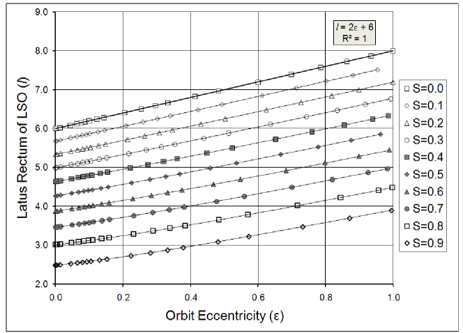
Figure 4: The LSO latus rectum, ${\tilde{l}}$, calculated for KBH systems in which the test-particle is in a prograde orbit.

[16, 8]; but we require additional formulae for KBH systems of various values of spin, and for the prograde and retrograde orbits. To this end, the algorithm outlined in Section 2.4.2 was used to calculate a sequence of latus rectum values, ${\tilde{l}}$, for LSOs of differing eccentricity, ${\varepsilon}$, in spherical coordinates. These results are plotted in Figures 4 and 5, for prograde and retrograde orbits respectively, and each set was fit to a sixth order polynomial equation of the form, ${\tilde{l}}={c}_{k}\,{\varepsilon}^{k}$, where ${c}_{k}$ corresponds to the coefficients to be calculated (see Tables 5 and 6). The result for the SBH system is shown in each of the two figures where the least squares fit yielded a linear result, ${\tilde{l}}=6.00+2.00\,{\varepsilon}$, which is consistent with equation (75). Such agreement is noteworthy because the least squares fit, based upon results previously known through the analytical and numerical analysis described in Section 2.4.2, corroborate the LSO relationship for the SBH.

The linear approximations obtained for the KBH systems were used to calculate the LSO radii which are essential for determining the point at which an inspiraling CO will plunge. Although the data point pairs, $\left(\varepsilon,\tilde{l}\right)$, derived for a particular spin became slightly nonlinear with increasing spin, the square of the correlation coefficient equals ${1}$.

Table 5: Results of polynomial fit applied to the retrograde numerical data plotted in Figure 5.

BH Spin ${\tilde{S}}$	Linear Formula for ${\tilde{l}}$		Higher Order Elements
	${\varepsilon}^{0}$	${\varepsilon}^{1}$	${\varepsilon}^{2}$	${\varepsilon}^{3}$	${\varepsilon}^{4}$	${\varepsilon}^{5}$	${\varepsilon}^{6}$
$0.9$ (ret)	$8.763688194$	$2.921197023$	$0.334533101$	$0.166029604$	$-0.090656413$	$0.038313748$
$0.8$ (ret)	$8.469624556$	$2.823177796$	$0.307860108$	$0.153608821$	$-0.083713859$	$0.035301568$
$0.7$ (ret)	$8.172997404$	$2.724303684$	$-0.279246699$	$0.140096895$	$-0.076041551$	$0.031871975$
$0.6$ (ret)	$7.873580734$	$2.624501799$	$-0.248523134$	$0.125602488$	$-0.068161649$	$0.028629143$
$0.5$ (ret)	$7.571112878$	$2.523682803$	$-0.215396442$	$0.109740157$	$-0.059474839$	$0.024985751$
$0.4$ (ret)	$7.265288032$	$2.421744495$	$-0.179553115$	$0.092264028$	$-0.049805202$	$0.020825353$
$0.3$ (ret)	$6.955745011$	2.318567387	$-0.140631846$	$0.072989398$	$-0.039242086$	$0.016335337$
$0.2$ (ret)	$6.6420520040$	$2.2140067262$	$-0.0981479990$	$0.0514756004$	$-0.0274318675$	$0.0112632939$
$0.1$ (ret)	$6.3236854510$	$2.1078897600$	$-0.0515364094$	$0.0274106312$	$-0.0145526678$	$0.0059528458$
$0.0$*	$6.0$	2.000000399	$-0.000004828$	$0.000019916$	$-0.000036936$	$0.000031685$	$0.001939522$

*Consistent with [16]; the nonlinear elements for ${\tilde{S}}=0.0$ were probably caused by round-off error.

Table 6: Results of polynomial fit applied to the prograde numerical data plotted in Figure 4.

BH Spin ${\tilde{S}}$	Linear Formula for ${\tilde{l}}$		Higher Order elements
	${\varepsilon}^{0}$	${\varepsilon}^{1}$	${\varepsilon}^{2}$	${\varepsilon}^{3}$	${\varepsilon}^{4}$	${\varepsilon}^{5}$	${\varepsilon}^{6}$
$0.0$*	$6.0$	2.000000399	$-0.000004828$	$0.000019916$	$-0.000036936$	$0.000031685$	$0.001939522$
$0.1$	$5.6701844450$	$1.8900661368$	$0.0575038413$	$-0.0317686472$	$0.0168080125$	$-0.0068645389$
$0.2$	$5.3331947130$	$1.7777446758$	$0.1223137900$	$-0.0688936900$	$0.0356024620$	$-0.0138446402$
$0.3$	$4.9876472960$	$1.6625673677$	$0.1965594291$	$-0.1141250883$	$0.0587798567$	$-0.0225955995$	$0.0044631526$
$0.4$	$4.6316401970$	$1.5439026552$	$0.2832200268$	$-0.1707514543$	$0.0874921671$	$-0.0327847030$
$0.5$	$4.2624301070$	$1.4208293794$	$0.3872264604$	$-0.2455511898$	$0.1262355513$	$-0.0461745401$
$0.6$	$3.8757931590$	$1.291939602$	$0.516967848$	$-0.350625042$	$0.181780713$	$-0.063577889$
$0.7$	$3.4645809000$	$1.154818226$	$0.689581456$	$-0.516713627$	$0.279766279$	$-0.096357483$
$0.8$	$3.0147269360$	$1.0047022061$	$0.9464897749$	$-0.8316991247$	$0.5056498507$	$-0.1870071888$
$0.9$	$2.4892766210$	$0.8291439890$	$1.4345599659$	$-1.6864540901$	$1.3351280439$	$-0.6279979225$	$0.1324275499$

*Consistent with [16]; the nonlinear elements for ${\tilde{S}}=0.0$ were probably caused by round-off error.

3 Conclusions

A knowledge of the relationship between the latus rectum, ${\tilde{l}}$, of a last stable orbit (LSO) and the Kerr black hole (KBH) spin, ${\tilde{S}}$, where ${\tilde{S}}=\left|\mathbf{J}\right|/{M}^{2}$, is essential for the calculation of the compact object (CO) orbit evolution in extreme black hole systems, and thus the gravitational wave energy emission. The Kerr metric provides the basis for the derivation of analytical relationships between orbital angular momentum squared (${\tilde{L}}^{2}$) and the apogee of the last stable orbit (${R_{Min}}$) for the prograde and retrograde elliptical orbits of test-particles about a KBH. These formulae lead directly to new and simplified representations of ${R_{LSO}}$ with respect to KBH spin for circular orbits, which in turn are used as a starting point in performing numerical analysis of elliptical LSOs. By using the prograde and retrograde relationships between the values of ${\tilde{L}}^{2}$ and ${R_{Min}}$ that we have derived from the effective potential, an elliptical LSO can be analysed numerically to yield values for ${R_{Min}}$. The algorithm provides a foundation that will be generalised to include inclined orbits for which the effective potential is more complicated than that for the case where the orbit lies in the equatorial plane of the KBH. Therefore finding the relationship between ${R}_{Min}$ and orbital angular momentum becomes paramount as it allow for the methodical treatment of orbits of successively greater eccentricity and orbital angular momentum.

Formulae for orbital energy, ${\tilde{E}}$, and the quantity, (${\tilde{L}}-{\tilde{S}}{\tilde{E}}$), have led us to the derivation of analytical expressions for ${\tilde{l}}$ in terms of ${\tilde{S}}$ and orbit eccentricity. The LSO values obtained by using these formulae were in excellent agreement with those in the literature, therefore, demonstrating their validity. The usefulness of these analytical expressions may be found in the advantage gained in future theoretical and numerical investigations. These equations and the others we have derived here also demonstrate the importance of using parameters that are normalised with respect to the KBH mass, ${M}$.

The values of ${R}_{Min}$ and ${R_{Max}}$, in Boyer-Lindquist (BL) coordinates, must be transformed to spherical coordinates. The ${\tilde{l}_{LSO(spherical)}}$ and LSO eccentricity (${\varepsilon}_{Spherical}$) can then be estimated and used in the integration of the post Newtonian orbital evolution equations. Because we can now calculate analytically the ${\varepsilon}_{Spherical}$ and ${\tilde{l}_{LSO(spherical)}}$ values for a range of KBH spins, ($0\leq{\tilde{S}}<1$; retrograde and prograde), it would facilitate the modelling of CO orbit evolution about a massive KBH.

The companion matrix (CM) has been shown to be of great use in finding the roots of complicated polynomials in an analytical form. The use of the CM in numerical work is also encouraging, especially because one can perform various linear operations on the CM in order to transform the final results.

Further investigation will be performed using the results of this work as a foundation. The methodologies that underlie our numerical algorithm will be extended to the case of inclined orbits. The radial frequency behaviour will also be treated by performing analytical integration of the radial path of the test-particle between the orbit pericentre and apocentre. The post Newtonian evolution equations that describe the inspiral of COs in extreme binary black hole systems will then be modelled.

The authors express their gratitude to Dr. L. Rezzolla for hosting P.G.K. at the Einstein Institute in Potsdam, Germany. P.G.K. thanks Western Science (UWO) for their financial support. M.H.’s research is funded through the NSERC Discovery Grant, Canada Research Chair, Canada Foundation for Innovation, Ontario Innovation Trust, and Western’s Academic Development Fund programs. S.R.V. acknowledges research funding by NSERC. The authors thankfully acknowledge Drs. N. Kiriushcheva and S. V. Kuzmin for their helpful discussions of the manuscript and I. Haque for help with the companion matrix method.

Appendix A: The Inverse Kerr Metric

The inverse Kerr metric expressed in the Boyer-Lindquist coordinates system. To simplify the presentation of the metric, we define the parameter:

$${\Sigma}={\rho}^{2} = {M^{2}}{\left(R^{2}+\tilde{S}^{2}{\cos^{2}\left(\theta\right)}\right)}.$$ (76)

The inverse Kerr metric is:

$${g}^{\delta\gamma}\Biggr{|}_{Kerr}$$ (77)

$$=\left({\Sigma}\right)^{-1} \left[{\begin{array}[]{cccc}{-\frac{{{\Sigma}\left(R^{2}+\tilde{S}^{2}\right)+2\,\tilde{S}^{2}R-2\,{\cos^{2}\left(\theta\right)}\tilde{S}^{2}R}}{{\left({R^{2}-2\,R+\tilde{S}^{2}}\right)}}}&0&0&\frac{-2\,{\tilde{S}R}}{{M}{\left({R^{2}-2\,R+\tilde{S}^{2}}\right)}}\\ 0&{R^{2}-2\,R+\tilde{S}^{2}}&0&0\\ 0&0&1&0\\ \frac{-2\,{\tilde{S}R}}{{M}{\left({R^{2}-2\,R+\tilde{S}^{2}}\right)}}&0&0&{\frac{{R^{2}-2\,R+\tilde{S}^{2}{\cos^{2}\left(\theta\right)}}}{{\left({R^{2}-2\,R+\tilde{S}^{2}}\right){\sin^{2}\left(\theta\right)}}}}\end{array}}\right].$$ (82)

In this study, $\theta=\frac{\pi}{2}$, therefore, the inverse Kerr metric simplifies to the form:

$${g}^{\delta\gamma}{\Biggr{|}}_{{Kerr}}$$ (83)

$$= \left[\begin{array}[]{cccc}-{\frac{{R}^{4}+{R}^{2}{\tilde{S}}^{2}+2\,{\tilde{S}}^{2}R}{\left({R}^{2}-2\,R+{\tilde{S}}^{2}\right){R}^{2}}}&0&0&-2\,{\frac{\tilde{S}}{{M}\left({R}^{2}-2\,R+{\tilde{S}}^{2}\right)R}}\\ \vskip 6.0pt plus 2.0pt minus 2.0pt\cr 0&{\frac{{R}^{2}-2\,R+{\tilde{S}}^{2}}{{R}^{2}}}&0&0\\ \vskip 6.0pt plus 2.0pt minus 2.0pt\cr 0&0&\frac{1}{{M}^{2}{R}^{2}}&0\\ \vskip 6.0pt plus 2.0pt minus 2.0pt\cr-2\,{\frac{\tilde{S}}{{M}\left({R}^{2}-2\,R+{\tilde{S}}^{2}\right)R}}&0&0&{\frac{{R}^{2}-2\,R}{\left({R}^{2}-2\,R+{\tilde{S}}^{2}\right){M}^{2}{R}^{2}}}\end{array}\right].$$ (88)

The determinant of the Kerr metric was calculated to be, $Det=-{\Sigma}^{2}{\sin^{2}\left(\theta\right)}.$

Appendix B: Use of the Companion Matrix to Solve a Quartic Equation

Given the task of finding the roots of a polynomial, (${p\left(R\right)=0}$), one might proceed by regarding it to be the characteristic polynomial of a matrix for which the eigenvalues are sought (i.e. the companion matrix) (see chapter 7 in [34]).

$$p\left(R\right) = \left({R}^{4}-12\,{R}^{3}-6\,{\tilde{S}}^{2}{R}^{2}+36\,{R}^{2}-28\,{\tilde{S}}^{2}R+9\,{\tilde{S}}^{4}\right)$$ (89)

$$= 0.$$

The creation of said matrix proceeds trivially to produce the companion matrix, ${M}$ (see section 7.4.6 in [34]):

$$M = \left[\begin{array}[]{cccc}0&0&0&-9\,{\tilde{S}}^{4}\\ \vskip 6.0pt plus 2.0pt minus 2.0pt\cr 1&0&0&28\,{\tilde{S}}^{2}\\ \vskip 6.0pt plus 2.0pt minus 2.0pt\cr 0&1&0&6\,{\tilde{S}}^{2}-36\\ \vskip 6.0pt plus 2.0pt minus 2.0pt\cr 0&0&1&12\end{array}\right],$$ (94)

from which one may calculate the eigenvalues. These eigenvalues represent the solutions of equation (89). There are four solutions, which are (in simplified form):

$${R} = 3\pm\sqrt{{Z}}\pm\sqrt{\frac{16{\tilde{S}}^{2}}{\sqrt{{Z}}}-{Z}+3\left(3+{\tilde{S}}^{2}\right)}$$ (95)

where

$${Z} = 3+{\tilde{S}}^{2}$$

$$+\left(3+{\tilde{S}}\right)\left(\left(1+{\tilde{S}}\right)\left(1-{\tilde{S}}\right)^{2}\right)^{\frac{1}{3}}$$

$$+\left(3-{\tilde{S}}\right)\left(\left(1-{\tilde{S}}\right)\left(1+{\tilde{S}}\right)^{2}\right)^{\frac{1}{3}}$$

We know by evaluating the solutions at ${\tilde{S}}=0$ (the Schwarzschild case) which two of the four solutions ought to be retained. They are:

$${R} = 3+\sqrt{{Z}}\pm\sqrt{\frac{16{\tilde{S}}^{2}}{\sqrt{{Z}}}-{Z}+3\left(3+{\tilde{S}}^{2}\right)}.$$ (96)

Appendix C: Use of the Companion Matrix to Find the Analytical Solution for ${\tilde{l}}_{LSO}$ for a General Elliptical Orbit

Treatment of the orbital energy, ${\tilde{E}}$, and the quantity, (${X}={\tilde{L}}-{\tilde{S}}{\tilde{E}}$), leads to an analytical expression for the latus rectum, ${\tilde{l}}$, of the last stable orbit (LSO) of a test-particle. An analytical form of ${\tilde{E}}$ (see [2]) is:

$${\tilde{E}} = \sqrt{1-\left(1-{\varepsilon}^{2}\right)\left(1-{\frac{{X}^{2}\left(1-{\varepsilon}^{2}\right)}{{\tilde{l}}^{2}}}\right){\tilde{l}}^{-1}}.$$ (97)

In Appendix A of [2] the term ${X}^{2}$ has been calculated to be,

$${X}^{2} = \frac{-{n}\mp\sqrt{d}}{2{f}},$$ (98)

for which the negative sign corresponds to a prograde orbit and the positive sign corresponds to a retrograde orbit. The functions in equation (98) are:

$${f} = {\frac{\tilde{l}\left(\tilde{l}-3-{\varepsilon}^{2}\right)^{2}-4\,{\tilde{S}}^{2}\left(1-\varepsilon\right)^{2}\left(1+\varepsilon\right)^{2}}{{\tilde{l}}^{3}}}$$ (99)

and

$${n} = -2\,{\frac{\tilde{l}\left(\tilde{l}-3-{\varepsilon}^{2}\right)+{\tilde{S}}^{2}\left(\tilde{l}+1+3\,{\varepsilon}^{2}\right)}{\tilde{l}}};$$ (100)

and the discriminator (${d}={n}^{2}-4{f}{c}$):

$${d} = \frac{16{\tilde{S}}^{2}}{{\tilde{l}}^{3}}\left(\tilde{l}\left(\tilde{l}-2-2\,\varepsilon\right)+{\tilde{S}}^{2}\left(1+\varepsilon\right)^{2}\right)\left(\tilde{l}\left(\tilde{l}-2+2\,\varepsilon\right)+{\tilde{S}}^{2}\left(1-\varepsilon\right)^{2}\right)$$ (101)

where

$${c} = \left({\tilde{l}}-{\tilde{S}}^{2}\right)^{2}.$$

The analytical relationship between ${\tilde{l}}_{LSO}$ of the LSO orbit and ${\tilde{S}}$ and ${\varepsilon}$ can be found by solving either of the following equalities:

$${\it{X_{{\it Prograde}}^{2}}}\left(1+\varepsilon\right)\left(3-\varepsilon\right) = {\tilde{l}}^{2}$$ (102)

and

$${\it{X_{Retrograde}^{2}}}\left(1+\varepsilon\right)\left(3-\varepsilon\right) = {\tilde{l}}^{2}.$$ (103)

By manipulating either of the equations (102) or (103) and removing the square root, one obtains the characteristic polynomial:

$$P\left({\tilde{l}}\right) = {\tilde{l}}^{4}+\left(-4\,\varepsilon-12\right){\tilde{l}}^{3}$$ (104)

$$+\left(-4\,{\tilde{S}}^{2}\varepsilon+2\,{\tilde{S}}^{2}{\varepsilon}^{2}-6\,{\tilde{S}}^{2}+4\,{\varepsilon}^{2}+24\,\varepsilon+36\right){\tilde{l}}^{2}$$

$$-4\,{\tilde{S}}^{2}\left(1+\varepsilon\right)\left({\varepsilon}^{2}+7\right)\tilde{l}+\left(1+\varepsilon\right)^{2}\left(-3+\varepsilon\right)^{2}{\tilde{S}}^{4}$$

$$= 0.$$

Converting the characteristic polynomial (equation (104)) into a companion matrix yields (see section 7.4.6 in [34]):

$${M} = \left[\begin{array}[]{cccc}0&0&0&-{\tilde{S}}^{4}\left(1+{\varepsilon}\right)^{2}\left(3-{\varepsilon}\right)^{2}\\ \vskip 6.0pt plus 2.0pt minus 2.0pt\cr 1&0&0&4\,{\tilde{S}}^{2}\left(1+{\varepsilon}\right)\left({\varepsilon}^{2}+7\right)\\ \vskip 6.0pt plus 2.0pt minus 2.0pt\cr 0&1&0&-2\,{\tilde{S}}^{2}{\varepsilon}^{2}+4\,{\varepsilon}\,{\tilde{S}}^{2}+6\,{\tilde{S}}^{2}-4\,{\varepsilon}^{2}-24\,\varepsilon-36\\ \vskip 6.0pt plus 2.0pt minus 2.0pt\cr 0&0&1&4\,(3+\varepsilon)\end{array}\right].$$ (109)

The eigenvalues of equation (109) can be evaluated analytically and they correspond to the roots of equation (104). Two of those roots correspond to the latus rectum (${\tilde{l}}$) of each of the prograde and retrograde test-particle orbits. One can also substitute the KBH spin, ${\tilde{S}}$, and the eccentricity of the orbit, ${\varepsilon}$, into the companion matrix and then calculate its eigenvalues to numerically calculate the values of ${\tilde{l}}$.

The analytical form of the eigenvalues is complicated; but a factorised form is presented here to illustrate how the solutions for ${\tilde{l}}$ were identified. The four eigenvalues, ${\lambda}_{i}$ (${i}=1..4$), are:

$${\lambda}_{i} = \left(3+\varepsilon\right)\pm\sqrt{Z_{{o}}}$$

$$\pm \sqrt{16\,{\frac{{\tilde{S}}^{2}\left(1+\varepsilon\right)}{\sqrt{Z_{{o}}}}}-Z_{{o}}+\left(3+\varepsilon\right)^{2}+{\tilde{S}}^{2}\left(1+\varepsilon\right)\left(3-\varepsilon\right)}.$$

By following the same reasoning as in Appendix B, we know that the solutions sought will each correspond to $6+2{\varepsilon}$ when ${\tilde{S}}=0$. In that case, ${Z}_{o}={\left(3+\varepsilon\right)^{2}}$, therefore, equation (Appendix C: Use of the Companion Matrix to Find the Analytical Solution for ${\tilde{l}}_{LSO}$ for a General Elliptical Orbit) simplifies to:

$${\lambda}_{i} = \left(3+\varepsilon\right)\pm\left(3+\varepsilon\right)\pm\left(0\right).$$ (111)

Therefore two of the eigenvalues, where ${\lambda}_{i}=0$, are excluded.

Figure 5: The LSO latus rectum, ${\tilde{l}}$, calculated for KBH systems in which the test-particle is in a retrograde orbit.

Figure 6: A comparison of orbits in BL and spherical coordinates for a KBH of spin, ${\tilde{S}}=0.5$ (prograde and retrograde). The view is taken from above the KBH equatorial plane. Orbital precession is not included.

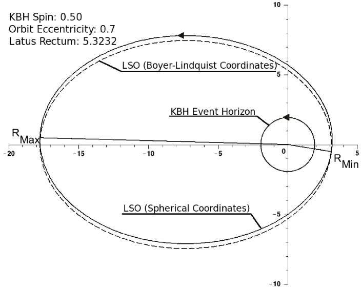
(a) Prograde

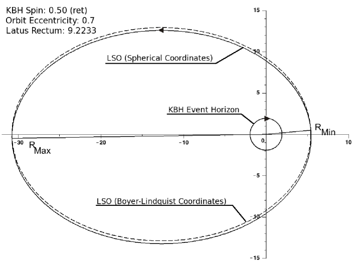
(b) Retrograde

Figure 7: A comparison of orbits in BL and spherical coordinates for a KBH of spin, ${\tilde{S}}=0.99$ (prograde and retrograde). The view is taken from above the KBH equatorial plane. Orbital precession is not included.

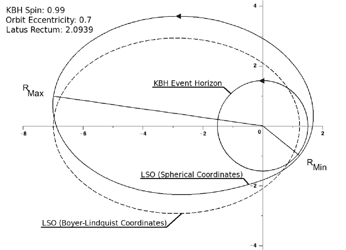
(a) Prograde

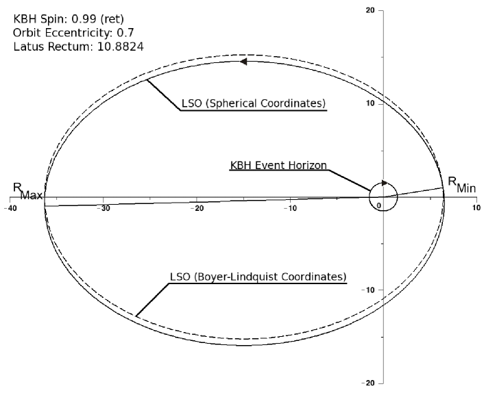
(b) Retrograde

References

- [1] K. S. Thorne. 300 Years of Gravitation. Cambridge, 1987.
- [2] K. Glampedakis and D. Kennefick. Zoom and whirl: Eccentric equatorial orbits around spinning black holes and their evolution under gravitational radiation reaction. Phys. Rev. D, 66(4):044002–+, August 2002.
- [3] F. A. Chishtie, S. R. Valluri, K. M. Rao, D. Sikorski, and T. Williams. The Analysis of Large Order Bessel Functions in Gravitational Wave Signals from Pulsars. Inter. J. Mod. Phys. D, 17(8):1197–1212, August 2008.
- [4] P. C. Peters and J. Mathews. Gravitational radiation from point masses in a keplerian orbit. Phys. Rev., 131(1):435–440, Jul 1963.
- [5] P. C. Peters. Gravitational radiation and the motion of two point masses. Phys. Rev., 136(4B):B1224–B1232, Nov 1964.
- [6] L. S. Finn. Detection, measurement, and gravitational radiation. Phys. Rev. D, 46:5236–5249, December 1992.
- [7] F. D. Ryan. Effect of gravitational radiation reaction on circular orbits around a spinning black hole. Phys. Rev. D, 52:3159, September 1995.
- [8] L. Barack and C. Cutler. Lisa capture sources: Approximate waveforms, signal-to-noise ratios, and parameter estimation accuracy. Phys. Rev. D, 69:082005, 2004.
- [9] Flanagan, É. É. and Hinderer, T. Evolution of the Carter constant for inspirals into a black hole: Effect of the black hole quadrupole". Phys. Rev. D, 75(12):124007, June 2007.
- [10] A. Ori and K. S. Thorne. Transition from inspiral to plunge for a compact body in a circular equatorial orbit around a massive, spinning black hole. Phys. Rev. D, 62(12):124022–+, December 2000.
- [11] W. Junker and G. Schaefer. Binary systems - Higher order gravitational radiation damping and wave emission. Mon. Not. R. astr. Soc., 254:146–164, January 1992.
- [12] V. A. Brumberg. Essential relativistic celestial mechanics. NASA STI/Recon Technical Report A, 92:40399–+, 1991.
- [13] S. A. Hughes, S. Drasco, É. É. Flanagan, and J. Franklin. Gravitational Radiation Reaction and Inspiral Waveforms in the Adiabatic Limit. Physical Review Letters, 94(22):221101–+, June 2005.
- [14] V. Pierro and I. M. Pinto. Exact solution of Peters-Mathews equations for any orbital eccentricity. Nuovo Cimento B Serie, 111:631–644, May 1996.
- [15] S. Chandrasekhar. The mathematical theory of black holes. Oxford/New York, Clarendon Press/Oxford University Press (International Series of Monographs on Physics. Volume 69), 1983, 663 p., 1983.
- [16] Curt Cutler, Daniel Kennefick, and Eric Poisson. Gravitational radiation reaction for bound motion around a schwarzschild black hole. Phys. Rev. D, 50(6):3816–3835, Sep 1994.
- [17] B. F. Schutz. A first course in general relativity. Cambridge, 17 edition, 2005.
- [18] S. L. Shapiro and S. A. Teukolsky. Black holes, white dwarfs, and neutron stars: The physics of compact objects. Research supported by the National Science Foundation. New York, Wiley-Interscience, 1983, 663 p., 1983.
- [19] James M. Bardeen, William H. Press, and Saul A Teukolsky. Rotating black holes: Locally nonrotating frames, energy extraction, and scalar synchrotron radiation. Astrophys. J., 178:347, 1972.
- [20] P. A. Sundararajan. Transition from adiabatic inspiral to geodesic plunge for a compact object around a massive Kerr black hole: Generic orbits. Phys. Rev. D, 77(12):124050–+, June 2008.
- [21] I. Ciufolini and E. C. Pavlis. A confirmation of the general relativistic prediction of the Lense-Thirring effect. Nature, 431:958–960, October 2004.
- [22] B. Mashhoon, F. W. Hehl, and D. S. Theiss. On the gravitational effects of rotating masses - The Thirring-Lense Papers. General Relativity and Gravitation, 16:711–750, August 1984.
- [23] I. Ciufolini. The 1995 - 99 measurements of the Lense-Thirring effect using laser-ranged satellites. Classical and Quantum Gravity, 17:2369–2380, June 2000.
- [24] I. Ciufolini. Dragging of inertial frames. Nature, 449:41–47, September 2007.
- [25] W. Schmidt. Celestial mechanics in Kerr spacetime. Classical and Quantum Gravity, 19:2743–2764, May 2002.
- [26] M. P. Hobson, G. Efstathiou, A. N. Lasenby, and L. H. Ford. General Relativity: An Introduction for Physicists, volume 60. 2007.
- [27] F. de Felice and C. J. S. Clarke. Relativity on Curved Manifolds. Relativity on Curved Manifolds, by F. de Felice and C. J. S. Clarke, pp. 459. ISBN 0521266394. Cambridge, UK: Cambridge University Press, May 1990., May 1990.
- [28] F. de Felice and G. Preti. On the meaning of the separation constant in the Kerr metric. Classical and Quantum Gravity, 16:2929–2935, September 1999.
- [29] L. E. Kidder, C. M. Will, and A. G. Wiseman. Spin effects in the inspiral of coalescing compact binaries. Phys. Rev. D, 47:4183, May 1993.
- [30] F. D. Ryan. Effect of gravitational radiation reaction on nonequatorial orbits around a kerr black hole. Phys. Rev. D, 53:3064–3069, 1996.
- [31] S. A. Hughes. Phys. Rev. D, 61:084004, 2000.
- [32] A. P. Lightman, W. H. Press, R. H. Price, and S. A. Teukolsky. Problem book in relativity and gravitation, volume 76. Princeton University Press (Princeton, New Jersey), 1975.
- [33] W. Rindler. The case against space dragging. Physics Letters A, 233:25–29, February 1997.
- [34] G. H. Golub and C. F. van Loan. Matrix computations. Matrix computations / Gene H. Golub, Charles F. Van Loan. Baltimore : Johns Hopkins University Press, 1996. (Johns Hopkins studies in the mathematical sciences), 1996.