Combinatorial Ricci Curvature and Laplacians for Image Processing

Abstract

A new Combinatorial Ricci curvature and Laplacian operators for grayscale images are introduced and tested on $2D$ synthetic, natural and medical images. Analogue formulae for voxels are also obtained. These notions are based upon more general concepts developed by R. Forman. Further applications, in particular a fitting Ricci flow, are discussed.

1 Introduction

Curvature analysis plays a major role in Image Processing, Computer Graphics, Computer Vision and their related fields, for many applications, such as reconstruction, segmentation and recognition, to list only a few (see, e.g. [4], [10], [16], [17]). Traditionally, the curvature estimation is that of a polygonal (polyhedral) mesh, approximating the ideally smooth ($\mathcal{C}^{2}$) image under study, such that the curvature measures of the mesh converge to the classical, differential, curvature measure of the investigated surface. For surfaces, by far the most important curvature is the intrinsic Gaussian (or total) curvature.

Recently, partly as an offshoot of the great interest generated by G. Perelman’s important contribution on the Ricci flow and its application in the proof of Thurston’s Geometrization Conjecture, and, implicitly of the Poincaré Conjecture (see, e.g. [12] for a comprehensive exposition), a flourishing of the study of various discrete versions of the Ricci flow (and similar related flows) occurred (see [3], [6], [8], [11]).

Ricci curvature measures the defect of the manifold from being locally Euclidean in various tangential directions. More precisely, it appears in the second term of the formula for the $(n-1)$-volume $\Omega(\varepsilon)$ generated within a solid angle (i.e. it controls the growth of measured angles) – see Fig. 1.

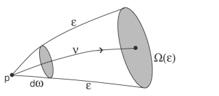
Figure 1: Ricci curvature as defect of the manifold from being locally Euclidean in various tangential directions (after Berger [1]). Here $d\omega$ denotes the $n$-dimensional solid angle in the direction of the vector ${\bf v}$, and $\Omega(\epsilon)$ the $(n-1)$-volume generated by geodesics of length $\varepsilon$ in $d\omega$.

Moreover,

$${\bf v}\cdot Ricci({\bf v})=\frac{n-1}{vol\big{(}\mathbb{S}^{n-2}\big{)}}\int_{{\bf w}\in T_{p}(M^{n}),\;{\bf w}\perp{\bf v}}\!\!\!\!\!K(<{\bf v},{\bf w}>)\,,$$

where $<{\bf v},{\bf w}>$ denote the plane spanned by ${\bf v}$ and ${\bf w}$, i.e. Ricci curvature represents an average of sectional curvatures. The analogy with mean curvature is further emphasized by the following remark: Ricci curvature behaves as the Laplacian of the metric $g$ (see, e.g. [2]). It is also important to note that in dimension $n=2$, that is in the case that is the most relevant for classical Image Processing and its related fields, Ricci curvature reduces to sectional (and scalar!) curvature, i.e. to the classical Gauss curvature.

However, both in the more classical context, as well as in the new directions mentioned above, smooth surfaces and/or their polygonal approximations considered. Unfortunately, smooth surfaces are at best a crude model (and usually nothing but a polite fiction), as far as digital and grayscale images, i.e. the standard objects of study in Image Processing, are considered, in particular for those objects that are not “natural images”, such as images produced using ultrasound imaging, MRI or CT. It would be of practical interest to define a proper notion of curvature for digital objects, in the spirit of [7]. By “proper” we mean discrete, intrinsic to the nature of the spaces under investigation, and not an approximation or rough discretization of a differential notion. Moreover, we hope that, by doing this, we shall be able to help bridge, at least partially, the divide between “Digital” and “Smooth” Image Processing. In addition, since,as we shall show, each dimension displays its own Laplacian, we believe our method can produce more types of heat flow, along edges, pixels, etc, thus allowing for better tools for the intelligence of higher dimensional data (such as RGB images, images with texture, etc.).

We are fortunate in our quest to be able to rely on the work of R. Forman [5] on Combinatorial Ricci curvature and the so called “Bochner Method”, where he addressed this very problem in the far more general setting of weighted cell complexes, which represent an abstractization of both polygonal meshes and weighted graphs. While we succinctly present some of the more general facts residing in Forman’s work, in this paper we concentrate solely on the case of grayscale images with their very special combinatorics and weights, and largely defer the study of higher dimensional (color) images and their curvatures and Laplacians for further study [15].

The present paper represents an extension of our previous work [14]. More precisely, we have augmented the previous version by adding: (a) The formula for the Ricci curvature of 3-dimensional cubical complexes (that is, in the case of images, for voxels); (b) A discussion on the purely combinatorial version of the Ricci curvature and Laplacians; (c) A theoretical comparison of the classical and combinatorial Laplacians; (d) A combinatorial diffusion, corresponding to upsampling and downsampling (this aspect being augmented by a computational example); (e) A discussion of a possible Ricci flow for our combinatorial setting, with a concrete suggested direction of study. In addition we have illustrated the meaning of Ricci curvature and included more detailed exposition of the Algebraic Topology background and ideas. And, last, but not least, we bring more (and new) experimental results: on synthetic images (that were not given previously), on standard test images and also on medical images.

2 Forman’s Combinatorial Ricci Curvature

We sketch below some of Forman’s main ideas [5]. This requires some technical definitions and notations. We do not introduce here the basic technical notions in Algebraic Topology and Differential Geometry, and refer the reader to [13] for the former and to [2] for the later.

To generalize the notion of Ricci curvature, in a manner that would include weighted cell complexes, one starts from the following form of the Bochner-Weitzenböck formula (see, e.g. [2]) for the Riemann-Laplace operator $\Box_{p}$ on $p$-forms on (compact) Riemannian manifolds:

$$\Box_{p}=dd^{*}+d^{*}d=\nabla_{p}^{*}\nabla_{p}+Curv(R)\,,$$ (1)

where $\nabla_{p}^{*}\nabla_{p}$ is the Bochner (or rough) Laplacian and where $Curv(R)$ is an expression with linear coefficients of the curvature tensor (Here $\nabla_{p}$ is the covariant derivative operator.) Of course, for cell-complexes one cannot expect such differentiable operators. However, a formal differential exists: in our combinatorial context (the operator) “$d$” being replaced by “$\partial$” – the boundary operator of the cellular chain complex (see [13]),

$$0\longrightarrow C_{n}(M,\mathbb{R})\stackrel{{\scriptstyle\partial}}{{\longrightarrow}}C_{n-1}(M,\mathbb{R})\stackrel{{\scriptstyle\partial}}{{\longrightarrow}}\cdots\stackrel{{\scriptstyle\partial}}{{\longrightarrow}}C_{0}(M,\mathbb{R})\longrightarrow 0\,,$$

were cells are playing in this setting the role of the forms in the classical (i.e. Riemannian) one. The following definition of the combinatorial Laplacian becomes now natural:

$$\Box_{p}=\partial\partial^{*}+\partial^{*}\partial:C_{p}(M,\mathbb{R})\rightarrow C_{p}(M,\mathbb{R})\,,$$ (2)

where $\partial^{*}:C_{p}(M,\mathbb{R})\rightarrow C_{p+1}(M,\mathbb{R})$ is the adjoint (or coboundary) operator of $\partial$, defined by: $<\partial_{p+1}c_{p+1},c_{p}>$ $=<c_{p+1},\partial_{p}^{*}c_{p}>_{p+1}\,,$ where $<\cdot,\cdot>=<\cdot,\cdot>_{p}$ is a (positive definite) inner product on $C_{p}(M,\mathbb{R})$, i.e. satisfying: (i) $<\alpha,\beta>=0,\forall\alpha\neq\beta$ and (ii) $<\alpha,\alpha>=w_{\alpha}>0$ – the weight of cell $\alpha$.

Forman [5] shows that an analogue of the Bochner-Weitzenböck formula holds in this setting, i.e. that there exists a canonical decomposition of the form:

$$\Box_{p}=B_{p}+F_{p}\,,$$ (3)

where $B_{p}$ is a non-negative operator and $F_{p}$ is a certain diagonal matrix. $B_{p}$ and $F_{p}$ are called, in analogy with the classical Bochner-Weitzenböck formula, the combinatorial Laplacian and combinatorial curvature function, respectively. Moreover, if $\alpha=\alpha^{p}$ is a $p$-dimensional cell (or $p$-cell, for short), then we can define the curvature function:

$$\mathcal{F}_{p}=<F_{p}(\alpha),\alpha>,$$ (4)

$F_{p}:C_{p}\rightarrow C_{p}$  being regarded as a linear function on $p$-chains. For dimension $p=1$ we obtain, by analogy with classical case, the following definition of discrete (weighted) Ricci curvature:

Definition 1

Let $\alpha=\alpha^{1}$ be a 1-cell (i.e. an edge). Then the Ricci curvature of $\alpha$ is defined as:

$${\rm Ric}(\alpha)=\mathcal{F}_{1}(\alpha).$$ (5)

While general weights are possible, making the combinatorial Ricci curvature extremely versatile, it turns out (see [5]), that it is possible to restrict oneself only to so called standard weights:

Definition 2

The set of weights $\{w_{\alpha}\}$ is called a standard set of weights iff there exist $w_{1},w_{2}>0$ such that given a $p$-cell $\alpha^{p}$, the following holds:

$$w(\alpha^{p})=w_{1}\cdot w_{2}^{p}\,.$$

(Note that the combinatorial weights $w_{\alpha}\equiv 1$ represent a set of standard weights, with $w_{1}=w_{2}=1$.) Using standard weights, we obtain the following formula for polyhedral (and in fact much more general) complexes:

$$\mathcal{F}(\alpha^{p})=w(\alpha^{p})\left[\left(\sum_{\beta^{p+1}>\alpha^{p}}\frac{w(\alpha^{p})}{w(\beta^{p+1})}+\sum_{\gamma^{p-1}<e_{2}}\frac{w(\gamma^{p-1})}{w(\alpha^{p})}\right)\right.$$ (6)

$$\left.-\sum_{\alpha_{1}^{p}\parallel\alpha^{p},\alpha_{1}^{p}\neq\alpha^{p}}\left|\sum_{\beta^{p+1}>\alpha_{1}^{p},\beta^{p+1}>\alpha^{p}}\frac{\sqrt{w(\alpha^{p})w(\alpha_{1}^{p})}}{w(\beta^{p+1})}-\sum_{\gamma^{p-1}<\alpha_{1}^{p},\gamma^{p-1}<\alpha^{p}}\frac{w(\gamma^{p-1})}{\sqrt{w(\alpha^{p})w(\alpha_{1}^{p})}}\right|\right],$$

where $\alpha<\beta$ means that $\alpha$ is a face of $\beta$, and the notation $\alpha_{1}\parallel\alpha_{2}$ signifies that the simplices $\alpha_{1}$ and $\alpha_{2}$ are parallel, the notion of parallelism being defined as follows:

Definition 3

Let $\alpha_{1}=\alpha_{1}^{p}$ and $\alpha_{2}=\alpha_{2}^{p}$ be two p-cells. $\alpha_{1}$ and $\alpha_{2}$ are said to be parallel ($\alpha_{1}\parallel\alpha_{2}$) iff either: (i) there exists $\beta=\beta^{p+1}$, such that $\alpha_{1},\alpha_{2}<\beta$; or (ii) there exists $\gamma=\beta^{p-1}$, such that $\alpha_{1},\alpha_{2}>\gamma$ holds, but not both simultaneously. (For example, in Fig. 1, $e_{1},e_{2},e_{3},e_{4}$ are all the edges parallel to $e_{0}$.)

Together with the formula above, the (dual) formula for the combinatorial Laplacian (see [5]) is also obtained to be:

$$\Box_{p}(\alpha_{1}^{p},\alpha_{2}^{p})=\sum_{\beta^{p+1}>\alpha_{1}^{p},\beta^{p+1}>\alpha_{2}^{p}}\epsilon_{\alpha_{1},\alpha_{2},\beta}\frac{\sqrt{w(\alpha_{1}^{p})w(\alpha_{2}^{p})}}{w(\beta^{p+1})}$$ (7)

$$\hskip 56.9055pt+\sum_{\gamma^{p-1}<\alpha_{1}^{p},\gamma^{p-1}<\alpha_{2}^{p}}\epsilon_{\alpha_{1},\alpha_{2},\gamma}\frac{w(\gamma^{p-1})}{\sqrt{w(\alpha_{1}^{p})w(\alpha_{2}^{p})}}\,,$$

where $\epsilon_{\alpha_{1},\alpha_{2},\beta},\epsilon_{\alpha_{1},\alpha_{2},\gamma}\in\{-1,+1\}$ depend on the relative orientations of the cells.

3 Combinatorial Ricci Curvature of Images

Before developing the relevant formulae in the special combinatorial setting of the tilling by squares of the plane, as it is usually considered in (Discrete) Image Processing, let us first indicate that it is advantageous to use standard weights. Such natural weights are proportional to the geometric content (s.a. length and area). It follows that the weight of any vertex is $w(v)=0$. Bearing this in mind, and considering the combinatorics of the square tilling (see Fig. 1), the specific form of Combinatorial Ricci curvature for $2D$ images is:

$${\rm Ric}(e_{0})=w(e_{0})\left[\left(\frac{w(e_{0})}{w(c_{1})}+\frac{w(e_{0})}{w(c_{2})}\right)-\left(\frac{\sqrt{w(e_{0})w(e_{1})}}{w(c_{1})}+\frac{\sqrt{w(e_{0})w(e_{2})}}{w(c_{2})}\right)\right]\,.$$ (8)

For the Laplacian there exists more than one possible choice, depending on the dimension $p$. The simplest, and operating on cells of the same dimensionality as the Discrete Ricci curvature, is $\Box_{1}$. Because vertices have weight $0$ and adjacent cells have opposite orientations, Equation (7) becomes, in this case (using the notation of Fig. 1):

$$\Box_{1}(e_{0})=\Box_{1}(e_{0},e_{0})=\frac{w(e_{0})}{w(c_{1})}-\frac{w(e_{0})}{w(c_{2})}.$$ (9)

The formula for the Combinatorial Bochner Laplacian follows immediately:

$$B_{1}(e_{0})=\Box_{1}(e_{0})-{\rm Ric}(e_{0})\,.$$ (10)

Instead of computing a Laplacian along the edge $e_{0}$, one can compute a Laplacian operating across the edge, namely $\Box_{2}(c_{1},c_{2})$. Since no 3-dimensional cells exist, the first sum in Equation (7) vanishes. Hence, we have (up to sign):

$$\Box_{2}(c_{1},c_{2})=\frac{w(e_{0})}{\sqrt{w(c_{1})w(c_{2})}}\,.$$ (11)

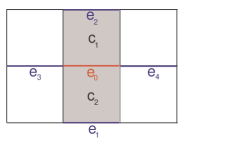
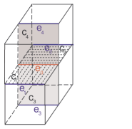
Figure 2: The elements appearing in the computation of the Combinatorial Ricci curvature of edge $e_{0}$ in the geometry of pixels.

Remark 1

By “weighing” the combinatorial formula for the curvature function $\mathcal{F}_{p}$ (cf, [5]) we obtain:

$$\mathcal{F}_{p}=\sharp\{\beta^{p+1}>\alpha\}+\sharp\{\gamma^{p-1}<\alpha\}-\sharp\{\delta\,|\,\delta\|\alpha\}.$$ (12)

(Here $\sharp X$ denotes the number of elements of the set $X$.) For $p=dim\,\alpha=1$, a simplified, purely combinatorial version of Formula (8) is also obtained:

$${\rm Ric}(e_{0})=w(c_{1})+w(c_{2})-w(e_{1})-w(e_{2})-w(e_{3})-w(e_{4})+2.$$ (13)

However, the above combinatorial version of the Ricci curvature does not provide considerable geometric insight and, therefore, does not yield interesting results.

In the case of the cubical geometric configuration present in Digital Images, Formula 6 becomes:

$${\rm Ric}(e_{0})=w(e_{0})\left[\left(\sum_{c^{2}>e_{0}}\frac{w(e_{0})}{w(c^{2})}+\sum_{c^{0}<e_{2}}\frac{w(c^{0})}{w(e_{0})}\right)\right.$$

$$\hskip 73.97733pt\left.-\sum_{e\parallel e_{0},e\neq e_{0}}\left|\sum_{c^{2}>e,c^{2}>e_{0}}\frac{\sqrt{w(e_{0})w(e)}}{w(c^{2})}-\sum_{c^{0}<e,c^{0}<e_{0}}\frac{w(c^{0})}{\sqrt{w(e_{0})w(e)}}\right|\right].$$

Since, as we have already noted, for digital images the vertices’ weights are always $0$, we obtain the following expression for ${\rm Ric}(e_{0})$:

$${\rm Ric}(e_{0})=w(e_{0})\left[w(e_{0})\left(\sum_{1}^{4}\frac{1}{w(c_{i})}\right)-\sqrt{w(e_{0})}\left(\sum_{1}^{4}\frac{\sqrt{w(e_{i})}}{w(c_{i})}\right)\right],$$ (14)

(see Fig. 2, right).

4 Experimental Results

Before commencing any experiments with the combinatorial Ricci curvature in the context of images, we had to choose a set of weights for the 2-, 1- and 0-dimensional cells of an image, that is for squares (pixels), their common edges and the vertices of the tilling of the image by the pixels. Any such choice should, obviously, be as natural and expressive as possible for image analysis. The choice of weights was motivated by two factors: the context of Image Processing, where a natural choice for weights imposes itself (see below) and the desire (and, indeed, sufficiency, see Section 2) to employ solely standard weights.

Since natural weights have to be proportional to the dimension of the cell, it follows immediately that the weight of any vertex (0-cell) has to be 0. Moreover, in the beginning, it is natural to choose $w_{1}=1$ and $w_{2}={\rm length\;of\;a\;cell}$. A somewhat less arbitrary choice for the length (i.e. basic weight) of an edge, would be ${\rm Length(e)=(dimension\;of\;the\;picture)^{-1}}$, hence that for the area (i.e. basic weight) of a pixel $\alpha$ being ${\rm Area(\alpha)=(dimension\;of\;the\;picture)^{-2}}$. The proper weight for a cell $\alpha$ should, however, take into account the gray-scale level (or height) $h_{\alpha}$ of the pixel in question, i.e. $w_{\alpha}=h_{\alpha}\cdot{\rm Area(\alpha)}$. This will become, so we hope, clearer in the following paragraph. The natural weight for an edge $e$ common to the pixels $\alpha$ and $\beta$ is $|h_{\alpha}-h_{\beta}|$. (A less “purely” combinatorial choice of cells and weights is discussed in [15].)

Note that, given an edge $e$, the Ricci curvature ${\rm Ric}(e)$ represents in a way a generalized mean of the weights the cells parallel to $e$. Therefore, it represents a measure of flow in the direction transversal to $e$. It follows, that, contrary perhaps to intuition, this type of Ricci curvature (and the Bochner Laplacian associated to it) in direction, say, parallel to the $x$-axis, is suitable for the detection of edges and ridges in the $y$-direction. On the other hand, since scalar (i.e. Gauss) curvature, is associated to each pixel, that is to each square of the tessellation, to compute the Gaussian curvature one has to compute the arithmetic mean of the Ricci curvatures of edges of the square under consideration – see Fig. 2. (A similar argument holds if one wishes to compute the 1-Laplacians, $\Box_{1}$ and $B_{1}$, of a given pixel.) The difference between the Ricci curvature computed in the horizontal and vertical directions, as well the “true”, i.e. average Ricci curvature can be seen in Fig. 3 and Fig. 4.

Figure 3: Computing the Ricci curvature for a pixel: Synthetic test image (left), Ricci curvature computed in horizontal (middle) and vertical (right) directions.

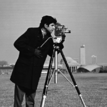
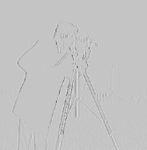
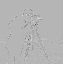
Figure 4: Computing the Ricci curvature for a pixel: The “Camera Man” test image (top, left), Ricci curvature computed in horizontal (top, right) and vertical (bottom, left) directions, and the Ricci (averaged) curvature (bottom, right).

As Fig. 5 illustrates, the Combinatorial Ricci curvature we introduced herein allows even for a non-optimal choice of weights, a very good approximation of Gaussian curvature of surfaces (i.e. for gray-scale images). Here, classical Gaussian curvature was computed using finite element methods standard in Image Processing – see [16].

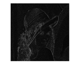
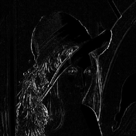
Figure 5: Gauss (left) and Combinatorial Ricci (right) comparison. Note the edge detecting capability if the Combinatorial Ricci curvature.

In contrast, both the Bochner (and Riemann) Laplacian sharply diverge from the classical one, e.g. the one obtained by using the standard Matlab function (see Fig. 6). This is not too surprising, given the fact that such a comparison is, in a sense, not relevant, due to the different dimensionality of the two concepts: The Combinatorial and Bochner Laplacian are, as stressed above, associated to edges, hence $1$-dimensional (this being underlined by the notation: $\Box_{1}(e_{0})$ and $B_{1}(e_{0})$, respectively). In contrast, the classical Laplacian is a pointwise function, (and, in its discrete setting, associated to the vertices of a mesh) hence $0$-dimensional. However, the Bochner Laplacian proves to be an excellent detector of “sharp” edges (see Fig. 7), therefore it may prove to be useful for contour detection and for segmentation.

Figure 6: Comparison of Different Laplacians: The Combinatorial (Forman) Laplacian $\Box_{1}(e_{0})$ (left), and the Bochner (rough) Laplacian $B_{1}(e_{0})$ (right). Note that the combinatorial Laplacians are good detectors of “sharp” edges.

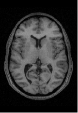
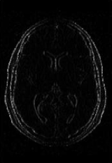
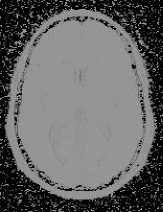
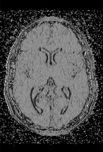
Figure 7: Axial brain scan image (top, left), its Combinatorial Ricci curvature (top, right), the Combinatorial (Forman) Laplacian $\Box_{1}(e_{0})$ (bottom, left), and the Bochner (rough) Laplacian $B_{1}(e_{0})$ (bottom, right). (Recall that $B_{1}(e_{0})=\Box_{1}(e_{0})-{\rm Ric}(e_{0})$.)

A “combinatorial diffusion” was also performed, either by upsampling, that is by division of the squares (pixels) into sub-squares of length $1/2$ or $1/3$, or by downsampling, i.e. by the fusion of 4 or 9 squares into larger ones. However, using the fusion of 9 squares produces more inferior results.) The weight after such upsampling would be, for instance $h_{\alpha}/4$. The effect of this last process on $\Box_{1}(e_{0})$ and on $B_{1}(e_{0})$ can be seen in Fig. 8.

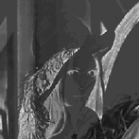
Figure 8: Comparison of Different Laplacians after upsampling, by fusion of 4 adjacent squares: From left to right: The Combinatorial (Forman) Laplacian $\Box_{1}(e_{0})$ (left), and the Bochner (rough) Laplacian $B_{1}(e_{0})$ (right).

5 Future Work

We briefly discuss below some of the natural and/or seemingly required directions of further study:

1. Evidently, the first task in testing the efficiency of the combinatorial Ricci curvature and Laplacian in medical imaging is to experiment with voxels, that is to apply the apparatus introduced herein to the analysis of volumetric data. Such 3- (and even 4-) dimensional manifolds and their evolution in time is most relevant, for instance, in the analysis of cardiac MRI. This brings us to the following point:

2. As already mentioned in the introduction, the full power of the Ricci curvature is revealed in the general heat-type diffusion and in discrete versions of the Ricci flow (and other related flows), that were introduced and experimented with elsewhere ([3], [6], [8], [11])). It is only natural to strive to develop and experiment with a discrete version of the Ricci flow corresponding to the combinatorial Ricci curvature introduced herein. The Ricci flow is given by

   $$\frac{\partial g}{\partial t}=-2{\rm Ric}(g(t))\,,$$

   where $g$ denotes the metric of the manifold. (see e.g. [12]). Various discretizations are possible for this flow. However, it seems that given the fact that the Combinatorial Ricci curvature is an edge measure, the most natural discretization in our context is the following one, inspired by [11] (see also [8]):

   $$\frac{\partial l_{ij}}{\partial t}=-2{\rm Ric}(e_{ij})\,,$$

   where $l_{ij}$ denotes the length of the edge $e_{ij}$. Experimental work on this type of flow is in progress [15].

3. As already noted, while we prefer, both for theoretical as well as for practical reasons, to work with standard weights, Forman’s combinatorial version of Ricci curvature is extremely versatile. Even if restricting oneself to using standard weights, i.e. proportional to the $p$-dimensional geometric content ($p$-volume), one still has freedom in choosing the weights $w_{2}$ and especially $w_{1}$ (see Section 2). Hence, to obtain best result, one can experiment in order to empirically determine, by using, e.g. variational methods, the optimal standard weights for a given application of the method.

4. The Combinatorial Laplacian is closely connected (by its very definition) to the cohomology groups of the cellular complex on which it operates (see [5]). It is natural, therefore, to apply the results and methods of [5] for the estimation of the dimension, and in some cases even the computation, of the cohomology groups (and by duality, of homology groups) of images. (See [9] on this direction of study in Image Processing.)

Acknowledgment

We would like to thank all our students who helped producing many of the images herein. The first author also wishes to express his gratitude to Professor Shahar Mendelson – his warm support is gratefully acknowledged. The research has been supported in part by Ollendorff Minerva Center for vision and Image Processing, Technion - Israel Institute of Technology.

References

- [1] Berger, M. Encounter with a Geometer, Part II, Notices of the AMS 47(3), 326-340, 2000.
- [2] Berger, M. A Panoramic View of Riemannian Geometry, Springer-Verlag, Berlin, 2003.
- [3] Chow, B. and Luo, F. Combinatorial Ricci Flows on surfaces, J. Differential Geometry 63, 97-129, 2003.
- [4] Dai J., Luo W., Yau S.-T. and Gu X. Geometric accuracy analysis for discrete surface approximation, Geometric Modeling and Processing, 59 72, 2006.
- [5] Forman, R. Bochner’s Method for Cell Complexes and Combinatorial Ricci Curvature, Discrete and Computational Geometry, 29(3), 323-374, 2003.
- [6] Glickenstein, D. A combinatorial Yamabe flow in three dimensions, Topology 44, 791-808, 2005.
- [7] Herman, G. T. Geometry of Digital Spaces, Birkhäuser, 1996.
- [8] Jin, M., Kim, J. and Gu, X. Discrete Surface Ricci Flow: Theory and Applications, Lecture Notes in Computer Science: Mathematics of Surfaces, 4647, 209-232, 2007.
- [9] Kaczynski, T., Mischaikow, K. and Mrozek, M. Computational homology, Springer-Verlag, New York, 2004.
- [10] Leibon, G. and Letscher, D. Delaunay Triangulations and Voronoi Diagrams for Riemannian Manifolds, Proceedings of the Sixteenth Annual Symposium on Computational Geometry, 341 - 349, 2000.
- [11] Luo, F. A combinatorial curvature flow for compact 3-manifolds with boundary, Electronic Research Announcemets of the AMS, 11, 12-20, 2005.
- [12] Morgan, J. and Tian, G. Ricci flow and the Poincare conjecture, Clay Mathematics Monographs 3, Providence, R.I., 2007.
- [13] Rourke, C. P. and Sanderson, B.J. Introduction to piecewise-linear topology, Springer-Verlag, Berlin, 1972.
- [14] Saucan, E., Appleboim, E., Wolansky, G and Zeevi, Y. Y. Combinatorial Ricci Curvature for Image Processing, Midas Journal, (http://hdl.handle.net/10380/1500), 2008.
- [15] Saucan, E., Appleboim, E., Wolansky, G and Zeevi, Y. Y. Combinatorial Ricci Flow for Image Processing, in preparation.
- [16] Saucan, E., Appleboim, E., and Zeevi, Y. Y. Sampling and Reconstruction of Surfaces and Higher Dimensional Manifolds, Journal of Mathematical Imaging and Vision, 30(1), 105-123, 2008.
- [17] Yakoya, N. and Levine, M. Range image segmentation based on differential geometry: A hybrid approach, IEEE Transactions on Pattern Analysis and Machine Intelligence, 11(6), 643-649, 1989.