Thermal transport in one-dimensional spin heterostructures

Abstract

We study heat transport in a one-dimensional inhomogeneous quantum spin $1/2$ system. It consists of a finite-size XX spin chain coupled at its ends to semi-infinite XX and XY chains at different temperatures, which play the role of heat and spin reservoirs. After using the Jordan-Wigner transformation we map the original spin Hamiltonian into a fermionic Hamiltonian, which contains normal and pairing terms. We find the expressions for the heat currents and solve the problem with a non-equilibrium Green’s function formalism. We analyze the behavior of the heat currents as functions of the model parameters. When finite magnetic fields are applied at the two reservoirs, the system exhibits rectifying effects in the heat flow.

I Introduction

In the last decade there has been a renewed interest related to the research of thermal transport in one-dimensional magnetic systems Solo ; dash . Most of these studies have been motivated by unusual high values of thermal conductance of some materials, as for example reported in Ref. lista2, . From the theoretical side, several works calculating and discussing thermal conductivity in different model Hamiltonians have also appeared lista5 , lista3 . On the other hand, spin Hamiltonians provide the natural scenario to implement quantum computation. This motivated interesting proposals of a variety of physical systems, like arrays of quantum dots, optical lattices and nuclear magnetic resonace experiments which are architectured to effectively behave like one-dimensional spin systems. design

Most of the theoretical studies on heat transport in spin systems are performed within the linear response regime, assuming a very small temperature gradient $\bigtriangledown T$, and using a Kubo formula. Altough this formula is widely used in calculating thermal transport properties it has several conceptual difficulties, particularly if $\bigtriangledown T$ is not small mahan ; dash . The thermal averaging assumes a constant temperature, and (as in all Kubo formulas), the time dependence is governed by the total Hamiltonian $H=H_{0}+H^{\prime}$, including the perturbation $H^{\prime}\sim\bigtriangledown T$ , while the thermodynamic averaging is done with $H_{0}$, assuming a fast evolution. For finite $\bigtriangledown T$ the separation of $H$ into an unperturbed part $H_{0}$ and a perturbation $H^{\prime}$ is in principle ambiguous. On the other hand, real experiments are performed by coupling the system under study to macroscopic systems with well defined temperatures that act as reservoirs. Therefore, it seems desirable to develop alternative approaches designed to treat systems out of equilibrium. Important progress has been achieved by studying the properties of non-equilibrium steady states of XX and XY chains within an algebraic setting which allows one to obtain explicit analytical expressions for different quantities such as entropy production pillet . Recently, the usefulness of Kubo formula for the investigation of heat transport in quantum systems has been discussed gemmer1 and the investigation of energy transport through spin systems beyond Kubo formula has been addressed on the basis of master equations and quantum Monte Carlo methods. gemmer2 Nevertheless, it is not clear how to extend these ideas to more general situations.

In this work we address the problem of thermal transport in one dimensional magnetic systems from a different perspective. We study a problem that to the best of our knowledge has not been considered yet. We study the heat flow through a spin chain heterostructure, which we generically define as a set of finite or semi-infinite spin chains attached by their ends. Each piece of the heterostructure can be in principle described by a different Hamiltonian. For definiteness, we shall consider in this work a finite central system connected to two (left and right) semi-infinite chains, with a finite temperature difference between themkarevski ; gemmer2 . This problem is the thermal analog of electronic transport through mesoscopic structures, nanodevices or molecules connected to conducting leads with a finite applied bias voltage, a subject of intense research in recent years. In fact, this type of set-up is the common situation found in the study of charge transport in electronic systems, where a central system is connected to charge reservoirs that also act as thermal baths. This is the basis of the ”Landauer” approach, which is one of the most common frameworks to study transport properties of meso- and nano- devices in the last years. transporte

In addition, as it is well known, one-dimensional spin $1/2$ systems can be mapped, via the Jordan-Wigner transformation to fermionic systems. Thus, the model under investigation is equivalent to an electronic heterostructure where very well established techniques, as the Schwinger-Keldysh non equilibrium Green’s functions method can be applied Kel .

We focus on a simple device where the central and right parts of the system can be described by XX spin 1/2 chains, and the left part corresponds to an anisotropic XY chain. The Jordan-Wigner transformation maps these models into bilinear fermionic systems, rendering the theoretical study simpler. We show that this simple device presents an interesting physical effect: due to a mechanism reminiscent of Andreev reflections in superconductors, this device could act as thermal diode. This rectifying effect might be useful for applications. We argue that this is a generic feature, which remains valid for anisotropic XYZ models.

The paper is organized as follows: in Section II we present the model, and the non-equilibrium formalism based on Green’s functions. Section III contains the numerical results. Section IV is a summary and discussion.

II The formalism

II.1 Model

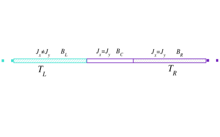
Figure 1: (Color online) Schematic digram showing the set up of the system. The right and central chains correspond to $XX$ models while the left chain is described by an $XY$ model. Left and right chains are taken semi-infinite at temperatures $T_{L}$ and $T_{R}$ respectively.

We consider a system of three one-dimensional spin 1/2 chains coupled through their ends as shown in Fig. 1. The system is described by the following Hamiltonian $H=H_{L}+H_{C}+H_{R}+H_{coup}$, where

$$H_{\alpha} = J_{\alpha}\sum_{i=1}^{N_{\alpha}-1}[S_{\alpha,i}^{x}S_{\alpha,i+1}^{x}+\lambda_{\alpha}S_{\alpha,i}^{y}S_{\alpha,i+1}^{y}]$$

$$-B_{\alpha}\sum_{i=1}^{N_{\alpha}}S_{\alpha,i}^{z},$$

$$H_{coup} = J^{\prime}[S_{L,1}^{x}S_{C,1}^{x}+S_{L,1}^{y}S_{C,1}^{y}]+$$ (1)

$$J^{\prime}[S_{R,1}^{x}S_{C,N_{C}}^{x}+S_{R,1}^{y}S_{N_{C},1}^{y}],$$

where in the first line, the index $\alpha=L,C,R$ (left, center, right) labels the different chains. Each chain is characterized by its nearest-neighbor exchange $J_{\alpha}$, with anisotropy $\lambda_{\alpha}$ for the ratio of the interaction along the $y$ direction with respect to that along $x,$ and the magnetic field $B_{\alpha}$ applied along the $z$ direction. The isotropic case for a given chain corresponds to $\lambda_{\alpha}=1$. The Hamiltonian $H_{coup}$ describes the coupling between the central chain, and the left and right ones. In terms of the representation for the spin operators: $S^{\pm}=S^{x}\pm iS^{y}$, the above Hamiltonian reads

$$H_{\alpha} = \frac{J_{\alpha}}{4}\sum_{l=1}^{N_{\alpha}-1}[(1-\lambda_{\alpha})(S_{\alpha,l}^{+}S_{\alpha,l+1}^{+}+S_{\alpha,l}^{-}S_{\alpha,l+1}^{-})$$

$$+(1+\lambda_{\alpha})(S_{\alpha,l}^{+}S_{\alpha,l+1}^{-}+S_{\alpha,l}^{-}S_{\alpha,l+1}^{+})]$$

$$-B_{\alpha}\sum_{l=1}^{N_{\alpha}}S_{\alpha,l}^{z},$$

$$H_{coup} = \frac{J^{\prime}}{2}[S_{L,1}^{+}S_{C,1}^{-}+S_{L,1}^{-}S_{C,1}^{+}]+$$ (2)

$$\frac{J^{\prime}}{2}[S_{R,1}^{-}S_{C,N_{C}}^{+}+S_{R,1}^{+}S_{N_{C},1}^{-}].$$

For the isotropic case, $\lambda_{\alpha}=1$ only the flip-flop terms with products of one raising and and one lowering spin operators survive.

We now introduce the Jordan-Wigner transformation to map the spin 1/2 Hamiltonian into a fermionic Hamiltonian through: $S_{\alpha,l}^{+}=f_{\alpha,l}^{\dagger}\exp(i\pi\sum_{j}^{\prime}f_{\alpha,j}^{\dagger}f_{\alpha,j})$, where $\sum_{j}^{\prime}$ denotes a sum over all the positions located at the left of the position $\alpha,l$. Similarly, the other spin operators transform as $S_{\alpha,l}^{-}=\exp(-i\pi\sum_{j}^{\prime}f_{\alpha,j}^{\dagger}f_{\alpha,j})f_{\alpha,l}$ and $S_{\alpha,l}^{z}=f_{\alpha,l}^{\dagger}f_{\alpha,l}-1/2$, where the operators $f_{l},f_{l}^{\dagger}$ obey fermionic commutation rules: $\{f_{\alpha,l},f_{\alpha^{\prime},l^{\prime}}^{\dagger}\}=\delta_{l,l^{\prime}}\delta_{\alpha,\alpha^{\prime}}$, and $\{f_{\alpha,l}^{\dagger},f_{\alpha^{\prime},l^{\prime}}^{\dagger}\}=\{f_{\alpha,l},f_{\alpha^{\prime},l^{\prime}}\}=0$. Substituting in the Hamiltonian (2), we get

$$H_{\alpha} = \sum_{l=1}^{N_{\alpha}-1}\{w_{\alpha}[f_{\alpha,l}^{\dagger}f_{\alpha,l+1}+f_{\alpha,l+1}^{\dagger}f_{\alpha,l}]$$

$$+\Delta_{\alpha}[f_{\alpha,l}^{\dagger}f_{\alpha,l+1}^{\dagger}+f_{\alpha,l+1}f_{\alpha,l}]\}$$

$$-\mu_{\alpha}\sum_{l=1}^{N_{\alpha}}f_{\alpha,l}^{\dagger}f_{\alpha,l},$$

$$H_{coup} = w^{\prime}[f_{L,1}^{\dagger}f_{C,1}+f_{C,1}^{\dagger}f_{L,1}]+$$ (3)

$$w^{\prime}[f_{C,N_{C}}^{\dagger}f_{R,1}+f_{R,1}^{\dagger}f_{C,N_{C}}],$$

where $w_{\alpha}=J_{\alpha}(1+\lambda_{\alpha})/4$, $\Delta_{\alpha}=J_{\alpha}(1-\lambda_{\alpha})/4$, $\mu_{\alpha}=B_{\alpha}^{z}$, and $w^{\prime}=J^{\prime}/2$. Therefore, in the language of fermionic operators, the Hamiltonian contains “normal”terms, with a creation and a destruction operator, as well as “anomalous” terms, with two creation or two destruction operators. The normal ones are a hopping term between nearest neighbors ($w_{\alpha}$), which is originated in the flip-flop spin terms and a chemical potential ($\mu_{\alpha}$) coupled to the fermionic density, which comes from the magnetic field pointing along the $z$-direction. The anomalous terms ($\Delta_{\alpha}$) are similar to those of a one-dimensional Hamiltonian with a gap function with $p$-wave symmetry, decoupled in the Bardeen-Cooper-Schrieffer (BCS) approximation and are originated by the anisotropy between the $X$ and $Y$ exchange interaction.

Inspired in this analogy, we focus our study on a junction between a chain with isotropic interactions ($XX$ spin chain) and an anisotropic one ($XY$ spin chain), which in the fermionic language is similar to a normal-superconductor junction. Such a situation is realized in a configuration with $\lambda_{R}=\lambda_{C}=0$ and $\lambda_{L}\neq 0$. We also assume that the left and right chains are at temperatures $T_{L}$ and $T_{R}$ respectively and they are both of infinite length( $N_{L}\rightarrow\infty$ and $N_{R}\rightarrow\infty$)

II.2 Energy balance

A consistent procedure to define an expression for the heat current from first principles, is to analyze the evolution of the energy stored in a small volume of the system and derive the corresponding equation for the conservation of the energy. liliheat For the present Hamiltonian we choose an elementary volume containing two nearest-neighbor positions of the chain. We place the volume enclosing the sites $l,l+1$ within the central (XX) chain, which in the fermionic language contains only normal terms. We work in units where $\hbar=1$. The equation for the conservation of the energy enclosed by this volume is

$$\frac{dE_{l,l+1}}{dt} = \frac{J_{C}}{2}\frac{d}{dt}\langle S_{l}^{+}S_{l+1}^{-}+S_{l}^{-}S_{l+1}^{+}\rangle-B_{C}^{z}\frac{d\langle S_{l}^{z}\rangle}{dt}$$ (4)

$$= w_{C}\frac{d}{dt}\langle f_{C,l}^{\dagger}f_{C,l+1}+f_{C,l+1}^{\dagger}f_{C,l}\rangle-$$

$$B_{C}^{z}\frac{d}{dt}\langle f_{C,l}^{\dagger}f_{C,l}\rangle$$

$$= -iw_{C}\langle[H,f_{C,l}^{\dagger}f_{C,l+1}+f_{C,l+1}^{\dagger}f_{C,l}]\rangle$$

$$+i\mu_{C}\langle[H,f_{C,l}^{\dagger}f_{C,l}]\rangle=J^{Q}_{l+1,l+2}-J^{Q}_{l-1,l},$$

where $J^{Q}_{l,l+1}$ is the heat current flowing from $l$ to $l+1$, which in the present setup coincides with the energy current. Its explicit expression is obtained from the evaluation of the above commutator, which gives

$$J^{Q} = J^{Q}_{l,l+1}=J^{Q}_{l-1,l}$$ (5)

$$= i\varepsilon_{l,l+1}^{C}(\varepsilon_{l-1,l}^{C}\langle f_{C,l-1}^{\dagger}f_{C,l+1}-f_{C,l+1}^{\dagger}f_{C,l-1}\rangle$$

$$+\varepsilon_{l+1,l+1}^{C}\langle f_{C,l+2}^{\dagger}f_{C,l+1}-f_{C,l+1}^{\dagger}f_{C,l+2}\rangle),$$

where $\varepsilon_{l,l^{\prime}}^{C}$ denotes the matrix element $l,l^{\prime}$ of the Hamiltonian $H_{C}$. In order to evaluate the above current it is convenient to introduce the lesser Green’s functions

$$G_{\alpha l,\beta l^{\prime}}^{<}(t,t^{\prime})=i\langle f_{\beta l^{\prime}}^{\dagger}(t^{\prime})f_{\alpha l}(t)\rangle,$$ (6)

thus

$$J^{Q} = 2\mbox{Re}\{\varepsilon_{l,l+1}^{C}G_{Cl+1,Cl-1}^{<}(t,t)\varepsilon_{l-1,l}^{C}$$ (7)

$$+\varepsilon_{l+1,l+1}^{C}G_{Cl+1,Cl+2}^{<}(t,t)\varepsilon_{l+2,l+1}^{C}\}.$$

The lesser Green’s functions are one of the basic elements within Keldysh non-equilibrium Green’s function formalism Kel . They are evaluated by solving the equations of motion (Dyson’s equations), which for our model can be written as follows

$$\sum_{k}G_{Cl,Ck}^{<}(\omega)[\delta_{k,l^{\prime}}\omega-\varepsilon_{k,l^{\prime}}^{C}]=0$$ (8)

for coordinates $l,l^{\prime}$ lying within the central chain. We have used the stationary property of the system, as a consequence of which the Green’s functions depend on the difference $t-t^{\prime}$, which allows us to transform: $G_{j,j^{\prime}}^{<}(t-t^{\prime})=\int_{-\infty}^{+\infty}d\omega/(2\pi)e^{-i\omega(t-t^{\prime})}G_{j,j^{\prime}}^{<}(\omega)$. Thus, using the above equation in Eq. (7) the energy current can be also expressed in the following way

$$J^{Q} = 2\mbox{Re}\{\int_{-\infty}^{+\infty}\frac{d\omega}{2\pi}\omega[\varepsilon_{l,l+1}^{C}G_{Cl+1,Cl}^{<}(\omega)$$ (9)

$$+\varepsilon_{l+1,l+1}^{C}G_{Cl+1,Cl+1}^{<}(\omega)]\}.$$

However $\mbox{Re}\{G_{j+1,j+1}^{<}(\omega)\}=0$. Thus, the heat current reduces to

$$J^{Q}=2\mbox{Re}\{\int_{-\infty}^{+\infty}\frac{d\omega}{2\pi}\omega\varepsilon_{l,l+1}^{C}G_{Cl+1,Cl}^{<}(\omega)\}.$$ (10)

Similarly, if we evaluate the heat current through the contacts $L-C$ and $C-R$, we find

$$J^{Q} = 2w^{\prime}\mbox{Re}\{\int_{-\infty}^{+\infty}\frac{d\omega}{2\pi}\omega G_{L1,C1}^{<}(\omega)\},$$ (11)

$$= 2w^{\prime}\mbox{Re}\{\int_{-\infty}^{+\infty}\frac{d\omega}{2\pi}\omega G_{CN,R1}^{<}(\omega)\}.$$

II.3 Solving Dyson’s equations

In order to evaluate $G^{<}$ and the heat current we follow a treatment close to that presented in Ref. lilisup, . We define the retarded “normal” and “Gorkov” Green’s functions

$$G_{\alpha l,\beta l^{\prime}}^{R}(t,t^{\prime}) = -i\Theta(t-t^{\prime})\langle\{f_{\alpha,l}(t),f_{\beta,l^{\prime}}^{\dagger}(t^{\prime})\}\rangle,$$

$$F_{\alpha l,\beta l^{\prime}}^{R}(t,t^{\prime}) = -i\Theta(t-t^{\prime})\langle\{f_{\alpha,l}^{\dagger}(t),f_{\beta,l^{\prime}}^{\dagger}(t^{\prime})\}\rangle.$$ (12)

Before writing down the Dyson’s equations satisfied the these “full”Green’s function let us define the following “free”particle $\hat{g}_{\alpha}^{0}(\omega)$ and hole $\hat{\overline{g}}_{\alpha}^{0}(\omega)$ Green’s functions

$$[\hat{g}_{\alpha}^{0}(\omega)]_{\alpha l,\alpha l^{\prime}}^{-1}=\delta_{l,l^{\prime}}(\omega+i\eta)-\varepsilon_{l,l^{\prime}}^{\alpha}$$

$$[\hat{\overline{g}}_{\alpha}^{0}(\omega)]_{\alpha l,\alpha l^{\prime}}^{-1}=\delta_{l,l^{\prime}}(\omega+i\eta)+\varepsilon_{l,l^{\prime}}^{\alpha},$$ (13)

with $\eta=0^{+}$.

From now on we will work in Fourier space and we will not write explicitly the $\omega$ dependence of Green’s functions unless necessary. For the left chain, we also define the functions $\hat{G}_{L}^{0}$, $\hat{\overline{G}}_{L}^{0}$ containing the paring term contribution, through the relations

$$[\hat{G}_{L}^{0}]^{-1}=[g_{L}^{0}]^{-1}-\hat{\Delta}_{L}\hat{\overline{g}}_{L}^{0}\hat{\Delta}_{L},$$

$$[\hat{\overline{G}}_{L}^{0}]^{-1}=[\overline{g}_{L}^{0}]^{-1}-\hat{\Delta}_{L}\hat{g}_{L}^{0}\hat{\Delta}_{L},$$ (14)

We also introduce

$$\hat{g}^{0}=\sum_{\alpha=L,C,R}\hat{g}_{\alpha}^{0},\;\;\hat{\overline{g}}^{0}=\sum_{\alpha=L,C,R}\hat{\overline{g}}_{\alpha}^{0},$$

$$\hat{G}^{0}=\hat{G}_{L}^{0}+\hat{g}_{C}^{0}+\hat{g}_{R}^{0},$$

$$\hat{\overline{G}}^{0}=\hat{\overline{G}}_{L}^{0}+\hat{\overline{g}}_{C}^{0}+\hat{\overline{g}}_{R}^{0},$$

$$\hat{F}_{L}^{0}=\hat{\overline{G}}^{0}\hat{\Delta}_{L}\hat{g}_{L}^{0},$$

$$\hat{\overline{F}}_{L}^{0}=\hat{G}^{0}\hat{\Delta}_{L}\hat{\overline{g}}_{L}^{0}.$$ (15)

Here $\varepsilon_{l,l^{\prime}}^{\alpha}$ and $\Delta_{\alpha l,\alpha l^{\prime}}$ are matrices defined on the coordinates of the chain $\alpha=L,C,$ or $R$, containing respectively, the normal and anomalous elements of the Hamiltonian. In the case we are studying only $\hat{\Delta}_{L}$ is non-vanishing.

To obtain these Green’s functions, we write the following Dyson’s equation which relate them with Green’s functions of the “disconnected” chains $\hat{g}_{\alpha}^{0}$ and $\hat{\overline{g}}_{\alpha}^{0}$ (see below) and the matrix elements of the contacts

$$\{[\hat{g}_{L}^{0}]^{-1}+[\hat{g}_{C}^{0}]^{-1}+[\hat{g}_{R}^{0}]^{-1}-$$

$$[\hat{W}]\}\hat{G}^{R}-\hat{\Delta}_{L}\hat{F}^{R}=\hat{1},$$ (16)

$$\{[\hat{\overline{g}}_{L}^{0}]^{-1}+[\hat{\overline{g}}_{C}^{0}]^{-1}+[\hat{\overline{g}}_{R}^{0}]^{-1}+$$

$$[\hat{W}]\}\hat{F}^{R}-\hat{\Delta}_{L}\hat{G}^{R}=\hat{0}.$$ (17)

The matrix $\hat{W}=\hat{W}_{L}+\hat{W}_{R}$ contains the matrix elements of $H_{cont}$ describing the connections between the central and left parts and between the central and right parts.

The above equations can be rewritten in a more convenient form by recourse to the following procedure. From Eq. (17)

$$\hat{F}^{R}=\hat{\overline{g}}^{0}[\hat{\Delta}_{L}\hat{G}^{R}-\hat{W}\hat{F}^{R}],$$ (18)

$$\hat{G}^{R}=\hat{g}^{0}+\hat{g}^{0}[\hat{\Delta}_{L}\hat{F}^{R}+\hat{W}\hat{G}^{R}],$$ (19)

Substituting (18) in (16) and (19) in (17) one obtains

$$\hat{G}^{R}=\hat{G}^{0}(1+\hat{W}\hat{G}^{R})+\hat{\overline{F}}_{L}^{0}\hat{W}\hat{F}^{R},$$ (20)

$$\hat{F}^{R}=\hat{F}_{L}^{0}(1+\hat{W}\hat{G}^{R})-\hat{\overline{G}}^{0}\hat{W}\hat{F}^{R},$$ (21)

Let us now consider Eq. (20) for the following particular coordinates

$$G_{Cl,Cl^{\prime}}^{R} = g_{C,l,l^{\prime}}^{0}+g_{C,l,1}^{0}w^{\prime}G_{L1,Cl^{\prime}}^{R}$$ (22)

$$+g_{C,l,N}^{0}w^{\prime}G_{R1,Cl^{\prime}}^{R},$$

$$G_{L1,Cl^{\prime}}^{R} = G_{L,1,1}^{0}w^{\prime}G_{C1,Cl^{\prime}}^{R}$$ (23)

$$+\overline{F}_{L,1,1}^{0}w^{\prime}F_{C1,Cl^{\prime}}^{R},$$

$$G_{R1,Cl^{\prime}}^{R} = g_{R,1,1}^{0}w^{\prime}G_{CN,Cl^{\prime}}^{R}.$$ (24)

Substituting Eqs. (23) and (24) in Eq. (22) it is easy to see that the Dyson’s equation for the two indices corresponding to coordinates of $C$ can be written as follows

$$\{[\hat{g}_{C}^{0}]^{-1}-\hat{\Sigma}^{R,gg}\}\hat{G}_{C}^{R}+\hat{\Sigma}^{R,gf}\hat{F}_{C}^{R}=\hat{1},$$ (25)

$$\{[\hat{\overline{g}}_{L}^{0}]^{-1}-\hat{\Sigma}^{R,ff}\}\hat{F}_{C}^{R}+\hat{\Sigma}^{R,fg}\hat{G}_{C}^{R}=\hat{0},$$ (26)

where the matrices of the above equations have sizes $N_{C}\times N_{C}$ and elements corresponding to the coordinates of the central chain. The “self-energy” matrices are

$$\Sigma_{l,l^{\prime}}^{R,ff} = \delta_{l,l^{\prime}}|w^{\prime}|^{2}[\delta_{l,1}\overline{G}_{L,1,1}^{0}+\delta_{l,N_{C}}\overline{g}_{R,1,1}^{0}$$

$$\Sigma_{l,l^{\prime}}^{R,gg} = \delta_{l,l^{\prime}}|w^{\prime}|^{2}[\delta_{l,1}G_{L,1,1}^{0}+\delta_{l,N_{C}}g_{R,1,1}^{0}]$$

$$\Sigma_{l,l^{\prime}}^{R,gf} = \delta_{l,l^{\prime}}|w^{\prime}|^{2}\delta_{l,1}\overline{F}_{L,1,1}^{0},$$

$$\Sigma_{l,l^{\prime}}^{R,fg} = \delta_{l,l^{\prime}}|w^{\prime}|^{2}\delta_{l,1}F_{L,1,1}^{0}.$$ (27)

The explicit expressions for these functions imply the evaluation of all the functions appearing in the right hand sides of (27). Notice that these functions have been defined from manipulations of the Dyson’s equations corresponding to $H_{L}$ or $H_{R}$ isolated from the central chain. We indicate a procedure for the calculation of these functions in appendix A. Note also that since the right and left parts of the system are held at two different but constant temperatures, these Green’s functions can be calculated at equilibrium. The advantage of the above representation becomes clear by writing (26) as

$$\hat{F}_{C}^{R}=\hat{\overline{g}}_{C}\hat{\Sigma}^{R,fg}\hat{G}^{R},$$

$$[\hat{\overline{g}}_{C}]^{-1}=[\hat{\overline{g}}_{C}^{0}]^{-1}-\hat{\Sigma}^{R,ff},$$ (28)

and substituting it in (25). The result leads to the solution of the retarded normal Green’s function within $C$

$$\hat{G}_{C}^{R} = \{[\hat{g}_{C}^{0}]^{-1}-\hat{\Sigma}_{\mbox{{\it eff}}}^{-1},$$

$$\hat{\Sigma}^{R}_{\mbox{{\it eff}}} = \hat{\Sigma}^{R,gg}+\hat{\Sigma}^{R,gf}\hat{\overline{g}}_{C}\hat{\Sigma}^{R,fg}.$$ (29)

The results obtained so far correspond to the retarded Green’s functions and self energies. The lesser Green’s function with coordinates within $C$ can be easily obtained by recourse to Langreth rules langr ; hern . In particular one obtains lilisup

$$\hat{G}_{C}^{<}=\hat{G}_{C}^{R}\hat{\Sigma}^{<}_{\mbox{{\it eff}}}\hat{G}_{C}^{A},$$ (30)

where the advanced Green’s function is obtained from the retarded one, by means of the relation $\hat{G}_{C}^{A}(\omega)=[\hat{G}_{C}^{R}(\omega)]^{\dagger}$ and the lesser component of the “self-energy” is

$$\hat{\Sigma}^{<}_{\mbox{{\it eff}}}=\hat{\Sigma}^{<,gg}+\hat{\Lambda}^{R}\hat{\Sigma}^{<,fg}+$$

$$\hat{\Sigma}^{<,gf}\hat{\Lambda}^{A}+\hat{\Lambda}^{R}\hat{\Sigma}^{<,ff}\hat{\Lambda}^{A},$$ (31)

with $\hat{\Lambda}^{R}(\omega)=\hat{\Sigma}_{\alpha}^{R,gf}(\omega)\hat{\overline{g}}_{C}(\omega)$ and $\hat{\Lambda}^{A}(\omega)=[\hat{\Lambda}^{R}(\omega)]^{\dagger}$. The self-energies have components

$$\Sigma_{l,l^{\prime}}^{<,\nu,\nu^{\prime}}(\omega)=i\delta_{l,l^{\prime}}[\delta_{l,1}\Gamma_{L}^{\nu,\nu^{\prime}}(\omega)f_{L}(\omega)+\delta_{l,N}\Gamma_{R}^{\nu,\nu^{\prime}}(\omega)f_{R}(\omega)]$$

being $\Gamma_{L}^{\nu,\nu^{\prime}}(\omega)=-2\mbox{Im}[\Sigma^{R,\nu\nu^{\prime}}(\omega)_{1,1}]$ and $\Gamma_{R}^{\nu,\nu^{\prime}}(\omega)=-2\mbox{Im}[\Sigma^{R,\nu\nu^{\prime}}(\omega)_{N,N}]$ with $\nu,\nu^{\prime}=g,f$. The Fermi functions $f_{\alpha}(\omega)$, with $\alpha=L,R$ depend on the temperatures $T_{L}$ and $T_{R}$ of the left and right chains respectively: $f_{\alpha}(\omega)=1/(1+e^{\omega/T_{\alpha}})$, in units where $k_{B}=1$.

Finally, the lesser counterparts of Eqs. (23) and (24), which correspond to Green’s functions with one of the coordinates in the central ($C$) chain and the other one in the left ($L$) or right ($R$) chain, can be calculated by recourse again to Langreth rules langr ; hern

$$G_{L1,Cl^{\prime}}^{<} = G_{L,1,1}^{0,<}w^{\prime}G_{C1,Cl^{\prime}}^{A}+G_{L,1,1}^{0,R}w^{\prime}G_{C1,Cl^{\prime}}^{<}$$ (32)

$$+\overline{F}_{L,1,1}^{0,<}w^{\prime}F_{C1,Cl^{\prime}}^{A}+\overline{F}_{L,1,1}^{0,R}w^{\prime}F_{C1,Cl^{\prime}}^{<},$$

$$G_{R1,Cl^{\prime}}^{<} = g_{R,1,1}^{0,<}w^{\prime}G_{CN,Cl^{\prime}}^{A}+g_{R,1,1}^{0,R}w^{\prime}G_{CN,Cl^{\prime}}^{<}.$$ (33)

II.4 Heat currents and transmission functions

We focus on the expression for the heat current evaluated in the contact between the central chain $C$ and $R$ given in Eq. (11). Using Eq. (33) one obtains

$$J^{Q} = -2|w^{\prime}|^{2}\int_{-\infty}^{+\infty}\frac{d\omega}{2\pi}\omega\mbox{Re}[G_{CN,CN}^{<}(\omega)g_{R,1,1}^{0,A}(\omega)$$ (34)

$$+G_{CN,CN}^{R}(\omega)g_{R,1,1}^{0,<}(\omega)].$$

Using (30) and after some algebra (see Ref. lilisup, ), it is found

$$J^{Q} = \int_{-\infty}^{+\infty}\frac{d\omega}{2\pi}\omega[f_{L}(\omega)-f_{R}(\omega)][T^{n}(\omega)-T^{a}(\omega)],$$

$$T^{n}(\omega) = \Gamma_{R}^{gg}(\omega)|G_{C,N,1}^{R}(\omega)|^{2}\Gamma_{L,{\mbox{\it eff}}}^{gg}(\omega),$$

$$T^{a}(\omega) = \Gamma_{R}^{gg}(\omega)|\overline{\Lambda}_{N,N}(\omega)|^{2}\Gamma_{R}^{ff}(\omega),$$ (35)

where

$$\Gamma_{L,\mbox{{\it eff}}}^{gg}=\Gamma_{L}^{gg}+2\mbox{Re}[\Gamma_{L}^{gf}\Lambda_{1,N}^{A}]+|\Lambda_{1,1}^{R}|^{2}\Gamma_{L}^{ff}+|\Lambda_{1,N}^{R}|^{2}\Gamma_{R}^{ff},$$

$$\overline{\Lambda}^{R}_{N,N}=G_{C,N,1}^{R}\Lambda^{R}_{1,N}.$$ (36)

The difference of Fermi functions in the expression of $J^{Q}$, reflects the fact that the existence of a non-vanishing heat current through the central system depends on the existence of a difference of temperatures between the left and right chains. The details of the model are enclosed in the behavior of the “normal” and “anomalous” transmission functions $T^{n}(\omega)$ and $T^{a}(\omega)$, which are analogous to those defined in Ref. lilisup, in the context of particle transport in a setup with normal and superconducting wires. The first function has, in fact, the structure of a transmission. Notice that it depends on the densities of states of the right and left chains through the functions $\Gamma_{R}$ and $\Gamma_{L}^{eff}$, and one the particle propagator between the first and last points of the central chain. Instead, $T^{a}(\omega)$ actually has the structure of a reflection process. Notice that it depends on the density of states for particles and holes of the right reservoir and on a multiparticle propagator $\overline{\Lambda}^{R}_{N,N}$ at the last point of the central chain. Typical plots for these functions are shown in Fig. 2. These functions do not depend on the temperatures $T_{L}$ and $T_{R}$ and are non-vanishing only within a finite range of energies of a width that is set by the largest exchange parameter between the left, right and central chains. These functions are symmetric with respect to $\omega=0$ for $B_{L}=B_{R}=0$ (see Fig. 2). This symmetry is broken for finite $B_{\alpha}$, since the effect of a finite magnetic field in one of the side chains is to shift the corresponding function as $\Gamma^{\nu\nu^{\prime}}_{\alpha}(\omega)\rightarrow\Gamma^{\nu\nu^{\prime}}_{\alpha}(\omega-B_{\alpha})$.

In the language of fermionic systems, two different kinds of processes take place in a normal-superconductor junction. For energies higher than the gap, the transport is due to the tunneling of normal single particle high-energy excitations. This mechanism contributes to the electronic transmission function $T^{n}(\omega)$. Instead, for low energies, below the gap, the transport is due to the mechanism known as “Andreev reflection”, which implies the combination of two fermions of the normal side into a Cooper pair within the superconducting one, leaving a hole that is reflected back from the junction into the normal side. Because of this mechanism, $T^{n}(\omega)\sim T^{a}(\omega)\sim 1$ for energies within the superconducting gap, i.e. $|\omega|\leq\Delta_{L}$. The effective conversion of electrons into Cooper pairs taking place in the mechanism of Andreev reflection helps to partice transport. Mathematically, this is reflected by the fact that the total particle transmission function is $T^{n}(\omega)+T^{a}(\omega)$. lilisup ; btk Instead, in the case of heat transport, $T^{a}(\omega)$ and $T^{n}(\omega)$ contribute with opposite sign, as explicitly shown in Eq. (35), i.e. the mechanism of Andreev reflection, plays a negative role regarding the heat transport. The consequence is a vanishing heat transport due to excitations within the energy window defined by the superconducting gap.

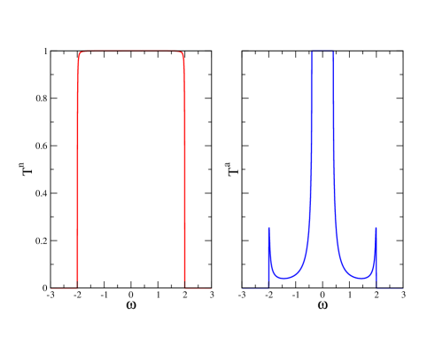
Figure 2: (Color online)“normal” (left) and “anomalous” (right) transmission functions. The latter is the counterpart to Andreev transmission function in electronic systems. Parameters are $\Delta_{L}=0.2$, $J_{L}=J_{R}=J_{C}=J^{\prime}=1$ and all chemical potentials set to zero.

In the original language of interacting spins, the above picture translates as follows. Low energy spin excitations traveling from the isotropic chain via flip-flop processes in the $z$ direction meet an energy gap at the other side of junction due to the anisotropic interaction which tends to favor flip-flop processes in a different direction. This favors the simultaneous raising or lowering of two spins at two neighboring positions of the chain and causes multiscattering processes in which a portion of the incident spin wave packet manages to twist and propagate into the other side, at the same time that a portion becomes reflected and propagates back.

We can describe the behavior of $J^{Q}$ for low $T$ and small temperature gradients $\delta T$ as follows. Writing $T_{R}=T$ and $T_{L}=T_{R}+\delta T$ we can approximate the difference of Fermi functions in Eq. (35) as

$$f_{L}(\omega)-f_{R}(\omega)\sim\frac{\partial f_{R}(\omega)}{\partial T}\delta T.$$ (37)

On the other hand, from Fig. 2, we can write,

$$T^{n}(\omega)-T^{a}(\omega)\sim 0 \omega\leq 2\Delta_{L}$$ (38)

$$T^{n}(\omega)-T^{a}(\omega)\sim 1 2\Delta_{L}\leq\omega\leq 2J$$ (39)

leading to,

$$J^{Q} = \frac{\delta T}{\pi}\int_{2\Delta_{L}}^{+2J}d\omega\omega\frac{\partial f_{R}(\omega)}{\partial T}$$ (40)

For low enough temperatures, $T\ll 2\Delta_{L}\ll 2J$, this expression can be further approximated as,

$$J^{Q} \sim \frac{\delta T}{\pi}\frac{\partial}{\partial T}\int_{2\Delta_{L}}^{\infty}d\omega\omega e^{-\beta\omega}$$ (41)

$$\sim \frac{4}{\pi}\delta T\frac{\Delta_{L}^{2}}{T}e^{-\frac{2\Delta_{L}}{T}}\;\;\;\;$$ (42)

Therefore, for $T<\Delta_{L}$, the heat current is exponentially small.

On the other hand, for $\Delta_{L}=0$, the behavior of the $J^{Q}$ is fully due to normal tunneling. For low $T$ we can perform a Sommerfeld expansion on the Fermi function to get

$$J^{Q} = \frac{2}{T^{2}}\delta T\frac{\partial}{\partial\beta}(\int_{0}^{+\infty}\frac{d\omega}{2\pi}\omega f(\omega)T^{n}(\omega))$$ (43)

$$\sim \frac{\pi}{3}T\delta T,\;\;\;\;T\ll J_{\alpha},\;\;\Delta_{L}=0.$$

III Results

In this section we discuss the behavior of the heat current as a function of the different ingredients of the spin system. For simplicity, we consider identical exchange parameters along the left, central and right chains: $J_{L}=J_{C}=J_{R}=J^{\prime}=J$. Without loss of generality we set $J=1$. Thus, we focus on a spin heterostructure with a single junction between a semi-infinite XX and a semi-infinite XY chain, which in the fermionic language translates to a single S-N junction. For this particular configuration, our results do not depend on the length of the central chain.

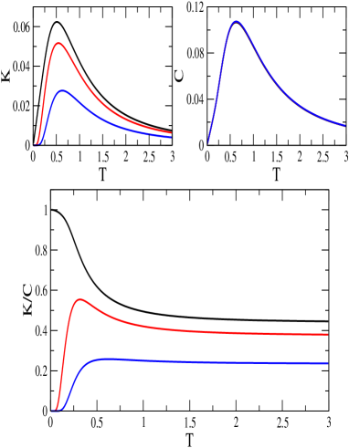
Figure 3: (Color online) Top left: Conductance, defined as the ratio of heat current to temperature gradient between right and left chains. Top right: specific heat of the central system. Bottom: ratio of the above magnitudes. Parameters are $T_{L}=T+\delta_{T},T_{R}=T$ where $\delta_{T}=0.005$, all chemical potentials set to zero, and (from top to bottom) $\Delta_{L}=0,0.25,0.5$.

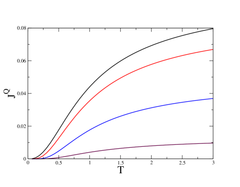
Figure 4: (Color online) Heat current as a function of the temperature of the left-chain (right chain at fixed $T_{R}=0$) for all chemical potentials set to zero, all hopping parameters set to 1 and different values of the paring parameter $\Delta_{L}$, from top to bottom $\Delta_{L}=0.1,0.25,0.5,0.75$.

As discussed in the previous subsection, the structure of the expression (35) for the heat current clearly reflects the fact that for small temperature differences, we obtain a behavior of the form

$$J^{Q}=-K\delta T,$$ (44)

where the coefficient $K$ can be interpreted as a thermal conductance. It is tempting to relate this coefficient with the conductivity $\kappa$ evaluated in several works on the basis of linear response theory. If we assume that the relation between the two coefficients is similar to the one between electrical conductance and electrical conductivity, $K$ and $\kappa$ should differ just by a geometrical factor. However, to the best of our knowledge, a rigorous relation between these two coefficients has not been presented in the literature. Nevertheless, the behavior of $K$ as a function of $T$ shown in the left upper panel of Fig. 3 for the case of two connected XX chains (see the plot corresponding to $\Delta_{L}=0$) is similar to the one reported in the literature for homogeneous and isotropic chains lista2 , lista5 ,lista3 . In this case, the anomalous component is zero and $K$ increases linearly in $T$ for low temperature [see Eq. (43)], as discussed at the end of the previous section. The conductance reaches a maximum at $T\sim J$. and decreases at higher temperatures, as a consequence of the finite bandwith (energy window) for the spin excitations amenable to cross the central chain transporting energy from one side to the other one. As expected, for a fixed temperature $K$ decreases for increasing values of $\Delta_{L}$. In agreement with the behavior discussed in the previous section, $K$ is exponentially small for $T<\Delta_{L}$ [see Eq. (40)], For higher temperatures, the high energy excitations are allowed to perform tunneling above the energy gap, with the concomitant increase of $K$. As in the case with $\Delta_{L}=0$, the maximum is achieved at $T\sim J$.

We also evaluate the specific heat for the equilibrium central system in contact to the side chains at the same temperature $T$ as follows:

$$C(T)=-\frac{2}{N}\sum_{l=1}^{N}\int_{-\infty}^{+\infty}\frac{d\omega}{2\pi}\frac{\partial f(\omega)}{\partial T}\omega\mbox{Im}[G^{R}_{C,l,l}(\omega)]$$ (45)

In a normal metallic system as described by Drude model, this quantity is related to the thermal conductivity through $\kappa=vlC/3$, being $v$ the Fermi velocity of the electrons and $l$ their mean free path aschcroft-mermin . We plot this quantity in the right upper panel of Fig. 3. This physical quantity is almost insensitive to the opening of the energy gap and the different plots, corresponding to different values of $\Delta_{L}$ almost coincide within the scale of the figure. From the lower panel of Fig. 3 we see that while for high temperatures there is a linear relation between $K$ and $C$, this is not the case at lower temperatures where Andreev type processes are relevant.

As stressed before, our calculation is not restricted to small temperature gradients. We show in Fig. 4 a plot of the heat current for several values of the anisotropy parameter $\Delta_{L}$ as a function of the temperature of the left chain while the temperature of the right chain $T$ is set fixed to zero. The figure clearly shows the suppression of the current as a consequence of the “Andreev reflection ”phenomena mentioned before. In fact for $T<\Delta_{L}$ the current is exponentially small, while it grows for higher temperatures.

Finally, in Fig. 5 we illustrate the behavior of the heat current when finite different magnetic fields are applied at the two side chains. The effect of applying magnetic fields at both sides of the junction leads to a interesting effect which me name “thermal diode effect”. As discussed in the previous section, a finite magnetic field originates a shift in the arguments of the functions $\Gamma_{\alpha}^{\nu\nu^{\prime}}(\omega)$, which leads to asymmetries in the transmission functions $T^{n}(\omega)$ and $T^{a}(\omega)$. For $\Delta_{L}=0$, only the normal transmission function and the functions $\Gamma^{gg}_{\alpha}(\omega)$ are non-vanishing. Furthermore, these functions are identical and gapless for $\alpha=L,R$. Therefore, the heat flow is perfectly antisymmetrical (the sign of the current is reversed preserving the absolute value) under the simultaneous change $T_{L}\leftrightarrow T_{R}$ and $B_{L}\rightarrow B_{R}$. Instead, for a finite $\Delta_{L}$, the situation changes. A gap opens for the excitations of the left chain and the functions $\Gamma^{\nu\nu^{\prime}}_{L}(\omega)=0$ vanish for $|\omega|<\Delta_{L}$, while the functions $\Gamma^{gg}_{R}(\omega)=\Gamma^{ff}_{R}(-\omega)$ remain finite. The consequence is an asymmetry in the behavior of the transmission functions under the change $B_{L}\rightarrow B_{R}$. The result is an effect of thermal rectification. That is, the magnitude of the current $J^{Q}$ when ($T_{L}=T$,$\mu_{L}=\mu$) and ($T_{R}=T^{\prime}$,$\mu_{R}=\mu^{\prime}$) is different to $J^{Q^{\prime}}$ when ($T_{L}=T^{\prime}$,$\mu_{L}=\mu^{\prime}$) and ($T_{R}=T$,$\mu_{R}=\mu$), which means that the device is more likely to conduct heat when the temperature difference is applied in one direction than in the other. We display the phenomena for two different values of $\Delta_{L}$. We show the current when ($\mu_{L}=0.3,T_{L}=T,\mu_{R}=0,T_{R}=0$) with dots and the current when ($\mu_{R}=0.3,T_{R}=T,\mu_{L}=0,T_{L}=0$) with a full line. When the value of $\Delta_{L}=0.2$ both currents are rather large and similar but when $\Delta_{L}=0.75$ the currents are smaller and clearly different.

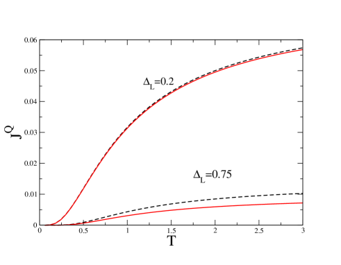
Figure 5: (Color online) Thermal Diode effect. We show the heat current when ($\mu_{L}=0.3,T_{L}=T,\mu_{R}=0,T_{R}=0$) (dotted line) and when ($\mu_{R}=0.3,T_{R}=T,\mu_{L}=0,T_{L}=0$) for two values of the pairing parameter $\Delta_{L}=0.2,0.75$

IV Summary and discussion

We have presented a theoretical framework to study heat transport in one-dimensional spin heterostructures.

In the present work we have focussed on a simple system composed of a junction between an anisotropic (XY) and an isotropic (XX) chain under the effect of an inhomogeneous magnetic field along the $z$ direction. Using the Jordan-Wigner transformation to map the problem into a fermionic system and using the non equilibrium Keldysh-Schwinger formalism we have obtained exact expression for the heat current in terms of Green’s functions of the ”disconnected” spin chain components. The resulting expressions can be evaluated numerically in a simple way. In the limits $\Delta_{L}\ll T\ll J$ and $T\ll\Delta_{L}\ll J$ explicit analytic expressions can also be given. We have studied the heat transport as a function of the different parameters of the model and we have shown that when different magnetic fields are applied at the end chains, a rectifying effect in the heat current occurs. This effect might be of interest for applications. Its origin can be traced back to the appearance of paring terms induced by the anisotropy parameter, which are in turn responsible for an Andreev reflection type mechanism.

In this work we have analyzed a simple model. However this methodology can be straightforwardly extended to more complex structures with many junctions and disorder. Our treatment relies on the Jordan-Wigner transformation which maps the original spin Hamiltonians into fermionic ones. In the case we have considered, the latter are bilinear. In more generic models, although we expect the rectifying effect still to be present, the technical analysis could be more complicated. For instance, in the isotropic Heisenberg model, which in addition to the exchange interaction along $x$ and $y$ directions, contains an additional exchange term along the $z$ direction, the Jordan-Wigner transformation translates such a term into a many-body fermionic interaction, which does not enable a straightforward analytical solution of the problem, as in the case we considered here. Nevertheless, the Green’s function formalism offers a framework for the construction of systematic approximations to treat those terms. Numerical methods could also be useful to deal with models containing many-body terms. feiguin As in electronic systems, many-body terms are expected to introduce further inelastic scattering processes, which could add further ingredients in addition to the transport mechanisms we have discussed here. We hope to report on some of these issues in future work.

Appendix A Green’s functions for an open chain with $p$-wave superconductivity

In this appendix we show a derivation of the Green’s functions $G_{L,1,1}^{0}(\omega)$, $\overline{G}_{L,1,1}^{0}(\omega)$, $F_{L,1,1}^{0}(\omega)$ and $\overline{F}_{L,1,1}^{0}(\omega)$, entering Eq. (27), which correspond to the end of a half infinite chain with $p$-wave superconductivity in the BCS approximation. Making the superconducting parameter $\Delta_{L}=0$, the first two Green’s functions give the corresponding result for the normal chain $g_{R,1,1}^{0}(\omega)$ and $\overline{g}_{R,1,1}^{0}(\omega)$ respectively.

The Green’s functions of the open chain can be solved considering a ring of $N$ sites, periodic except for the fact that the energy at one site (which we label as site 0) is increased by an energy $A$, and then taking the limit $N,A\rightarrow+\infty$. The Hamiltonian is

$$H = \sum_{l=0}^{N-1}\{w[f_{l}^{\dagger}f_{l+1}+f_{l+1}^{\dagger}f_{l}]$$ (46)

$$+\Delta[f_{l}^{\dagger}f_{l+1}^{\dagger}+f_{l+1}f_{l}]\}$$

$$-\mu\sum_{l=0}^{N-1}f_{l}^{\dagger}f_{l}+Af_{0}^{\dagger}f_{0}.$$

We have solved the problem using two different methods: i) solving the equations of motion in Fourier space, and ii) solving a Dyson’s equation that relates the above Green’s functions to those of the periodic chain ($A=0$) which can be obtained easily using Bloch theorem. Both results of course coincide, but the latter method involves a simpler algebra. We define a matrix

$$\tilde{G}=\left(\begin{array}[]{cc}G_{L,1,1}^{0}(\omega)&F_{L,1,1}^{0}(\omega)\\ \overline{F}_{L,1,1}^{0}(\omega)&\overline{G}_{L,1,1}^{0}(\omega)\end{array}\right),$$ (47)

with the Green’s functions for $A\neq 0$, and a corresponding matrix $\tilde{g}$ for $A=0$. These matrices are equivalent to the ones obtained by using Nambu’s representation for the Hamiltonian and the Green’s functions. cuevas From the equations of motion of these Green’s functions, one obtains

$$\tilde{G}=\tilde{g}+\tilde{g}\tilde{A}\tilde{G}\text{,}$$ (48)

where $\tilde{A}$, is proportional to $A$.

Solving Eq. (48) for $\tilde{G}$ and taking the limit $A\rightarrow+\infty$ the following expressions result

$$G_{L,1,1}^{0} = h_{0}(\omega)-\frac{h_{1}^{2}(\omega)}{h_{0}(\omega)}-\frac{h_{2}^{2}(\omega)}{h_{0}^{\ast}(-\omega)}.$$ (49)

$$F_{L,1,1}^{0} = h_{2}(\omega)\left(\frac{h_{1}^{\ast}(-\omega)}{h_{0}^{\ast}(-\omega)}-\frac{h_{1}(\omega)}{h_{0}(\omega)}\right).$$ (50)

$$\overline{G}_{L,1,1}^{0}(\omega)=-(G_{L,1,1}^{0})^{*}(-\omega)\,\,\,\overline{F}_{L,1,1}^{0}=-(F_{L,1,1}^{0})^{*}(-\omega)$$ (51)

The $h$-functions entering the second members of Eqs. (49) and (50) are Green’s functions of the periodic chain and can be calculated easily in Fourier space. The result is

$$h_{0}(\omega) = \frac{1}{N}\sum_{k}\frac{\omega+\epsilon_{k}}{\omega^{2}-\epsilon_{k}^{2}-\Delta_{k}^{2}},$$

$$h_{1}(\omega) = \frac{1}{N}\sum_{k}\frac{(\omega+\epsilon_{k})\cos k}{\omega^{2}-\epsilon_{k}^{2}-\Delta_{k}^{2}},$$

$$h_{2}(\omega) = \frac{1}{N}\sum_{k}\frac{2\Delta\sin^{2}k}{\omega^{2}-\epsilon_{k}^{2}-\Delta_{k}^{2}},$$ (52)

where in the second members $\omega$ includes an infinitesimally small imaginary part, $\epsilon_{k}=2w\cos k-\mu$, and $\Delta_{k}=2\Delta\sin k$.

For $N\rightarrow+\infty$, the sums can be replaced by integrals. Decomposing the integrands into a sum of simple fractions with denominators linear in $\cos k$ and numerators independent of $k$, the integrals can be evaluated analytically using gra

$$I(b)=\frac{1}{\pi}\int_{0}^{\pi}\frac{dk}{\cos k+b}=\frac{1}{\sqrt{b^{2}-1}},$$ (53)

where the sign of the root is determined by the sign of the imaginary part of the second member.

Defining

$$\tilde{\omega} = \frac{\omega}{2w},\text{ }\tilde{\Delta}=\frac{\Delta}{w},\text{ }\tilde{\mu}=\frac{\mu}{2w},\text{ }d=1-\tilde{\Delta}^{2},$$

$$r = \left[(\tilde{\omega}^{2}-\tilde{\Delta}^{2})d+(\tilde{\Delta}\tilde{\mu})^{2}\right]^{1/2}/d.$$

$$b_{1} = \tilde{\mu}/d-r,\text{ }b_{2}=\tilde{\mu}/d+r,$$

$$d_{1} = \left[4wrd\right]^{-1},$$ (54)

the result takes the form

$$h_{0}(\omega) = d_{1}[(r-\tilde{\omega}-\tilde{\mu}\tilde{\Delta}^{2}/b)I(b_{1})$$

$$+(r+\tilde{\omega}+\tilde{\mu}\tilde{\Delta}^{2}/b)I(b_{2})],$$

$$h_{1}(\omega) = -d_{1}\{2r-[(r-\tilde{\omega}-\tilde{\mu}\tilde{\Delta}^{2}/b)b_{1}I(b_{1})$$

$$+(r+\tilde{\omega}+\tilde{\mu}\tilde{\Delta}^{2}/b)b_{2}I(b_{2})]\},$$

$$h_{2}(\omega) = d_{1}\tilde{\Delta}\{2r+[I(b_{1})]^{-1}-[I(b_{2})]^{-1}\}.$$ (55)

References

- (1) For a recent review see for instance, A. V.Sologubenko, T. Lorenz, H. R. Ott, A. Freimuth, J. Low Temp. Phys. 147, 387 (2007). See also, X. Zotos, P. Prelovsek, in ”Interacting Electrons in Low Dimensions”, book series ”Physics and Chemistry of Materials with Low-Dimensional Structures”, Kluwer Academic Publishers (2003),
- (2) Abhishek Dhar, Advances In Physics, 57, 457 (2008).
- (3) A. V. Sologubenko, E. Felder, K. Giannò, H. R. Ott, A. Vietkine, and A. Revcolevschi, Phys. Rev. B 62, R6108 (2000); A. V. Sologubenko, K. Giannò, H. R. Ott, A. Vietkine, and A. Revcolevschi, ibid. 64, 054412 (2001); A. V. Sologubenko, H. R. Ott, G. Dhalenne, and A. Revcolevschi, Europhys. Lett. 62 540 (2003).
- (4) For some recent works on spin chain and ladders see for instance, F.Heidrich-Meisner, A. Honecker, and W. Brenig, Phys. Rev. B 71, 184415 (2005); A. V. Rozhkov and A. L. Chernyshev , Phys. Rev. Lett. 94, 087201 (2005); P. Jung, R. W. Helmes, and A. Rosch, Phys. Rev. Lett. 96, 067202 (2006); K. Louis, P. Prelovsek and X. Zotos, Phys. Rev. B 74, 235118 (2006); P. Jung and A. Rosch, Phys. Rev. B 75, 245104 (2007); E. Boulat, P. Mehta, N. Andrei, E. Shimshoni, and A. Rosch, Phys. Rev. B 76, 214411 (2007); A. V. Savin, G. P. Tsironis, and X. Zotos, Phys. Rev. B 75, 214305 (2007)
- (5) See also, H. Castella, X. Zotos, and P. Prelovsek, Phys. Rev. Lett. 74, 972 (1995); S. Fujimoto and N. Kawakami, J. Phys. A 31, 465 (1998); X. Zotos, Phys. Rev. Lett. 82, 1764 (1999);T. Prosen and D. K. Campbell, Phys. Rev. Lett. 84, 2857 (2000); J. V. Alvarez and C. Gros, Phys.Rev. Lett 88, 077203 (2002); E. Shimshoni, N.Andrei, and A. Rosch, Phys. Rev. B 68, 104401 (2003); K. Saito, Phys. Rev. B 67, 064410 (2003); F.Heidrich-Meisner, A. Honecker, D.C. Cabra, and W. Brenig, Phys. Rev. B 66, 140406(R) (2002), Phys. Rev. B 68, 134436 (2003), Phys. Rev. Lett. 92, 069703 (2004) E. Orignac, R.Chitra, R.Citro, Phys. Rev. B 67, 134426 (2003); X. Zotos, Phys. Rev. Lett. 92, 067202 (2004).
- (6) H. M. Pastawski, P. R. Levstein, and G. Usaj, Phys. Rev. Lett. 75, 4310 (1995); D. Loss and D. P. DiVincenzo, Phys. Rev. A 57, 120 (1998); T. S. Cubitt and J. I. Cirac, Phys. Rev. Lett. 100, 180406 (2008) and references therein.
- (7) G.D. Mahan, Many Particle Physics (Kluver/Plenum, New York, 2000).
- (8) W.Aschbacher and C.A.Pillet, J.Stat.Phys. 112, 1153 (2003), Y.Ogata, Phys. Rev. 66, 066123 (2002), Y.Ogata, Phys. Rev. 66, 016135 (2002).
- (9) M. Michel, G. Mahler, and J. Gemmer, Phys. Rev. Lett. 95, 180602 (2005); J. Gemmer, R. Steinigeweg, and M. Michel, Phys. Rev. B 73, 104302 (2006).
- (10) M. Michel, O. Hess, H. Wichterich, and J. Gemmer, Phys. Rev. B 77, 104303 (2008).
- (11) For other type of baths see D.Karevski and T.Platini, unpublished.
- (12) S. Datta, Electronic Transport in Mesoscopic Systems (Cambridge University press, 1995);Y. Imry, Introduction to Mesoscopic Physics, (Oxford University Press, 1997).
- (13) J. Rammer and H. Smith, Rev. Mod. Phys. 58, 323 (1986).
- (14) L. Arrachea, M. Moskalets and L. Martin-Moreno, Phys. Rev. B 75, 245420 (2007); L. Arrachea and M. Moskalets, cond-mat/0903.1153.
- (15) L. Arrachea, Phys. Rev. B, in press, cond-mat/0811.1648.
- (16) D.C. Langreth, in Linear and Non-Linear Transport in Solids, J.T. Devreese, E. Van Dofen (Eds.), (Plenum Press, New York, 1076).
- (17) A. Hernández, V. M. Apel, F. A. Pinheiro, and C. H. Lewenkopf, Physica A 385, 148 (2007).
- (18) G. E. Blonder, M. Tinkham, and T. M. Klapwijk, Phys. Rev. B 25, 4515 (1982).
- (19) N.W.Ashcroft and N. D. Mermin, ”Solid State Physics”, Holt, Rinehart and Winston. 1976.
- (20) J. C. Cuevas, A. Martín-Rodero, and A. Levy Yeyati, Phys. Rev. B, 54, 7366 (1996).
- (21) I.S. Gradshtein and I.M. Ryzhik, Tables of Integrals, Series and Products (Academic Press, New York, 1980)
- (22) A. E. Feiguin, S. R. White, and D. J. Scalapino, Phys. Rev. B. 75, 024505 (2007); A. E. Feiguin, S. R. White, D. J. Scalapino, and I. Affleck; Phys. Rev. Lett. 101, 217001 (2008);