Gossip Coverage Control for Robotic Networks:
Dynamical Systems on the Space of Partitions

Abstract

Future applications in environmental monitoring, delivery of services and transportation of goods motivate the study of deployment and partitioning tasks for groups of autonomous mobile agents. These tasks are achieved by recent coverage algorithms, based upon the classic methods by Lloyd. These algorithms however rely upon critical requirements on the communication network: information is exchanged synchronously among all agents and long-range communication is sometimes required. This work proposes novel coverage algorithms that require only gossip communication, i.e., asynchronous, pairwise, and possibly unreliable communication. Which robot pair communicates at any given time may be selected deterministically or randomly. A key innovative idea is describing coverage algorithms for robot deployment and environment partitioning as dynamical systems on a space of partitions. In other words, we study the evolution of the regions assigned to each agent rather than the evolution of the agents’ positions. The proposed gossip algorithms are shown to converge to centroidal Voronoi partitions under mild technical conditions.

Our treatment features a broad variety of results in topology, analysis and geometry. First, we establish the compactness of a suitable space of partitions with respect to the symmetric difference metric. Second, with respect to this metric, we establish the continuity of various geometric maps, including the Voronoi diagram as a function of its generators, the location of a centroid as a function of a set, and the widely-known multicenter function studied in facility location problems. Third, we prove two convergence theorems for dynamical systems on metric spaces described by deterministic and stochastic switches.

1 Introduction

In the not too distant future, networks of coordinated autonomous robots will perform a broad range of environmental monitoring and logistic tasks. Robotic camera networks will monitor airports and other public infrastructures. Teams of vehicles will perform surveillance, exploration and search and rescue operations. Groups of robots will enable novel logistic capacities in the transportation of goods and the delivery of services and resources to customers. New applications will be enabled by the ongoing decreases in size and cost and the increases in performance of sensors, actuators, communication devices and computing elements.

In these future applications, load balancing algorithms will dictate how the workload is shared amongst and assigned to the individual robots. In other words, robotic resources will be assigned and deployed to competing requests in such a way as to optimize some performance metric. Remarkably, load balancing problems in robotic networks are often equivalent to robotic deployment and environment partitioning problems. For example, in surveillance applications, optimal sensor coverage is often achieved by partitioning the environment and assigning individual robotic sensors to individual regions of responsibility. Similarly, in the transportation of goods or delivery of services, minimizing the customer wait-time is equivalent to a multi-vehicle routing problem and, in turn, to computing optimal depot positions and regions of responsibility.

Motivated by these scenarios, this paper considers the two following interrelated problems. The deployment problem for a robotic network amounts to the design of coordination algorithms that lead the robots to be optimally placed in an environment of interest. Deployment performance is characterized by an appropriate network utility function that measures the deployment quality of a given configuration. The partitioning problem is the design of coordination algorithms that lead the robots to optimally partition the environment into subregions of interest; even here the objective is usually achieved through the design of appropriate utility functions.

Literature review

A wide range of literature is relevant to our investigation. In next four paragraphs we review previous work on centroidal Voronoi partitions, distributed robotic deployment, animal territory partitioning, and mathematical modeling tools.

The “centering and partitioning” algorithm originally proposed by Lloyd [25] and elegantly reviewed in the survey [14] is a classic approach to facility location and environment partitioning problems. The Lloyd algorithm computes centroidal Voronoi partitions as optimal configurations of an important class of objective functions, called multicenter functions. Besides their intended application to quantization theory [18], centroidal Voronoi partitions have widespread applications in numerous disciplines, including statistical pattern recognition [22], mathematical imaging [15], geometric optimization [3] and spatial resource allocation [12]. Recent mathematical interest has focused on convergence analysis [13], bifurcation analysis of low dimensional problems [38], and anisotropic partitions [16], among other topics.

Distributed and robotic versions of the Lloyd algorithm have been recently developed in the multiagent literature; see the survey [28] and the text [9, Chapter 5 and literature notes in Section 5.4]. We briefly review this growing literature in what follows. Generalized centroidal Voronoi partitions are shown in [17] to be asymptotically optimal for estimation of stochastic spatial fields by sensor networks. In [10] convergence results are obtained for simple basic interactions among mobile agents such as “move away from the closest other agent” or “move toward the furthest vertex of your region of responsibility.” Convergence to centroidal Voronoi partitions is established in [4] for a class of communication-less sensor-based algorithms (related to the classic clustering work by MacQueen [27]). In [36] adaptive coverage controls are proposed for environments described by unknown density functions. Dynamic environments and corresponding dynamic coverage problems are treated in [21]. In [31] partitioning policies are shown to achieve optimal load balancing in vehicle routing problems, i.e., problems in which a robotic network provides service to customers that arrive in real time in the environment.

Territory partitioning via competitive behaviors is a classic subject of study in behavioral ecology; see [1] for a comprehensive survey. For example, it is known [2] that the foraging behavior of conflicting colonies of red harvester ants (Pogonomyrmex barbatus) results in non-overlapping dominance regions that resemble Voronoi partitions. Non-overlapping dominance regions akin to centroidal Voronoi partitions are well documented in [6, 37, 14] for the mouthbreeder fish (Tilapia mossambica). Territoriality behavior and competition among prides of African lions (Panthera leo) are discussed in [29]. Overall, numerous animal species achieve territory partitioning without a central coordinating entity and without synchronized communication, but rather relying upon asynchronous accidental interactions and stigmergy. To the best of our knowledge about biological and engineering multiagent systems, asynchronous territory partitioning has been barely studied, see [37] for introductory ideas about animal behavior, and mathematical models and analysis are lacking.

To finalize the literature review, here is a synopsis of the mathematical ideas from diverse disciplines that we bring to bear on deployment and partitioning problems. First, we adopt the so-called gossip communication model, in which only peer-to-peer asynchronous communication links are required. This communication model is widely studied in the wireless communication literature; example references include [23, 7]. Moreover, we consider control systems on a non-Euclidean state space; the interest for non-Euclidean spaces has a rich history in nonlinear control theory, dynamical systems and robotics, including the early work [8] and a recent application to multiagent systems [35]. Finally, we adopt various tools from topology and from the study of hyperspaces of sets [30].

Statement of contributions

This paper uncovers novel mathematical principles and tools of relevance in coordination problems and multiagent systems.

We tackle partitioning and coverage control algorithms in innovative ways. First, we design algorithms that require only gossip communication, i.e., asynchronous, pairwise, and possibly unreliable communication. Gossip communication is a simple, robust and effective protocol for noisy and uncertain wireless environments. Gossip communication may be implemented in wandering robots with short-range unreliable communication (see the illustrative motion coordination strategy in Appendix A). Second, we propose a paradigm shift in coverage control and multicenter optimization. Classically [10, 17, 21, 28, 31, 36, 38], the state space for the coverage algorithms are the agents’ positions, i.e., as a function of the agents’ positions the environment is divided into regions and regions are assigned to each agent. Instead, in our approach, the agents’ positions are no longer a concern: the state space is the space of partitions of the environment and the algorithm dictates how to update the regions.

Within the innovative context of gossip communication and partition-based mechanisms, we devise a novel algorithm for multicenter and coverage optimization. Our gossip coverage algorithm is a peer-to-peer version of Lloyd algorithm and aims to compute centroidal Voronoi partitions. Which robot pair communicates at any given time is the outcome of either a deterministic or a stochastic process. We also propose a modified version that restricts communication exchanges to adjacent regions and that has suitable continuity properties. Simulations illustrate that our algorithms successfully compute centroidal Voronoi partitions.

To formally establish the convergence properties of our proposed gossip coverage algorithms, we perform a detailed mathematical analysis composed of three steps. First, we develop suitable versions of the Krasovskii-LaSalle invariance principle for dynamical systems on metric spaces described by deterministic and stochastic switches. Convergence to a set of fixed points is achieved under a uniform deterministic or stochastic persistency condition. Second, we establish the continuity of various geometric maps, including (1) the Voronoi diagram as a function of its generators, (2) the location of the generalized centroid as a function of a set, (3) the widely-known multicenter function studied in facility location, and (4) the gossip coverage algorithms. These continuity properties are established with respect to the symmetric distance metric in the space of partitions. Third and final, we study the topology of the space of partitions. With respect to the symmetric difference metric we prove the compactness of a relevant subset of partitions. Specifically, we focus on partitions whose component regions are the union of a bounded number of convex sets.

In summary, relying upon our extensions of the invariance principle, the compactness of a subset of the set of partitions, and the continuity of the various relevant maps, we establish the convergence properties of the proposed gossip algorithms. In short, the algorithms converge to the set of centroidal Voronoi partitions under mild technical assumptions and under the assumption that the gossip communication exchanges satisfy either a deterministic or a stochastic persistency condition.

Organization and notations

The paper is structured as follows. In Section 2 we review multicenter optimization and coverage control ideas. In Section 3 we state our asynchronous territory partitioning problem, provide a solution via the gossip coverage algorithm, state the convergence properties of the algorithm and report some simulation results. The following Sections 4, 5 and 6 develop the mathematical machinery required to prove the convergence results. Section 4 contains the convergence theorems extending the Krasovskii-LaSalle invariance principle. Section 5 contains a discussion about the compactness properties of the space of partitions. Section 6 states the continuity properties of the relevant maps and functions and contains the proof of the main convergence results. Concluding remarks are given in Section 7.

We let $\mathbb{R}_{>0}$ and $\mathbb{R}_{\geq 0}$ denote the set of positive and non-negative real numbers, respectively, and $\mathbb{Z}_{\geq 0}$ denote the set of non-negative integer numbers. Given $A\subset\mathbb{R}^{d}$, we let $\operatorname{int}(A)$, $\overline{A}$, $\partial A$ and $\operatorname{diam}(A)$ denote its interior, its closure, its boundary and its diameter, respectively. Given two sets $X$ and $Y$, a set-valued map $T:X\rightrightarrows Y$ associates to an element of $X$ a subset of $Y$.

2 A review of multicenter optimization and distributed coverage control

In this section we review a variety of known results in geometric optimization and in robotic coordination. In Subsection 2.1 we review the notion of environment partitions and we introduce the multicenter function as a way to define optimal environment partitions and optimal robot or sensor positions in the environment. In Subsection 2.2 we review some distributed control algorithms for agent motion coordination and environment partitioning based on the classic Lloyd algorithm.

2.1 Partitions, centroids and multicenter optimization

We let $Q$ denote an environment of interest to be apportioned. We assume $Q$ is a compact convex subset of $\mathbb{R}^{d}$ with non-empty interior. Partitions of $Q$ are defined as follows.

Definition 2.1 (Partition)

An $N$-partition of $Q$, denoted by $v=(v_{i})_{i=1}^{N}$, is an ordered collection of $N$ subsets of $Q$ with the following properties:

1. $\operatorname{\cup}_{i\in\{1,\dots,N\}}v_{i}=Q$;

2. $\operatorname{int}(v_{i})\operatorname{\cap}\operatorname{int}(v_{j})$ is empty for all $i,j\in\{1,\dots,N\}$ with $i\not=j$; and

3. each set $v_{i}$, $i\in\{1,\dots,N\}$, is closed and has non-empty interior.

The set of $N$-partitions of $Q$ is denoted by $\mathcal{V}_{N}$.

Let $p=(p_{1},\ldots,p_{N})\in Q^{N}$ denote the position of $N$ agents in the environment $Q$. Given a group of $N$ agents and an $N$-partition, each agent is naturally in one-to-one correspondence with a component of the partition; specifically we refer to $v_{i}$ as the dominance region of agent $i\in\{1,\dots,N\}$.

On $Q$, we define a density function to be a bounded measurable positive function $\phi:Q\rightarrow\mathbb{R}_{>0}$ and a performance function to be a locally Lipschitz, monotone increasing and convex function $f:\mathbb{R}_{\geq 0}\rightarrow\mathbb{R}_{\geq 0}$. With these notions, we define the multicenter function $\mathcal{H}_{\textup{multicenter}}:\mathcal{V}_{N}\times Q^{N}\rightarrow\mathbb{R}_{\geq 0}$ by

$$\mathcal{H}_{\textup{multicenter}}(v,p)=\sum_{i=1}^{N}\int_{v_{i}}f(\|p_{i}-q\|)\phi(q)dq.$$ (1)

This function is well-defined because closed sets are measurable. We aim to minimize $\mathcal{H}_{\textup{multicenter}}$ with respect to both the partition $v$ and the locations $p$.

Remarks 2.2 (Locational optimization)

As discussed in the introduction and in the survey [14], the multicenter function $\mathcal{H}_{\textup{multicenter}}$ has numerous interpretations. Here we review two applications entailing robotic networks. First, in a vehicle routing and service delivery example [31], given vehicles at locations $p_{i}$, assume that $f(\|p_{i}-q\|)$ is the cost incurred by agent $i$ to travel to service an event taking place at point $q$. Events take place inside $Q$ with likelihood $\phi$. Accordingly, $\mathcal{H}_{\textup{multicenter}}$ quantifies the expected wait-time between event arrivals and agents servicing them.

Second, in an environmental monitoring application [28], assume the robots aim to detect acoustic signals that originate and propagate isotropically in the environment. Because of noise and loss of resolution, the ability to detect a sound source originating at a point $q$ from a sensor at position $p_{i}$ is proportional to the signal-to-noise ratio (which degrades with $\|q-p_{i}\|$). If the performance function $f$ equals minus the signal-to-noise ratio, then $\mathcal{H}_{\textup{multicenter}}$ quantifies the expected signal-to-noise ratio and detection capacity for acoustic signals generated at random locations. $\square$

Among all possible ways of partitioning a subset of $\mathbb{R}^{d}$, one is worth of special attention. Define the set of partly coincident locations $S_{N}=\{p\in Q^{N}\,|\;p_{i}=p_{j}\text{ for some }i,j\in\{1,\dots,N\},\,i\not=j\}$. Given $p\in Q^{N}\setminus S_{N}$, the Voronoi partition of $Q$ generated by $p$, denoted by $V(p)$, is the ordered collection of the Voronoi regions $\big{(}V_{i}(p)\big{)}_{i=1}^{N}$, defined by

$$V_{i}(p)=\{q\in Q\,|\;\|q-p_{i}\|\leq\|q-p_{j}\|\text{ for all }j\neq i\}.$$ (2)

In other words, the Voronoi partition is a map $V:(Q^{N}\setminus S_{N})\rightarrow\mathcal{V}_{N}$. The regions $V_{i}(p)$, $i\in\{1,\dots,N\}$, are convex and, if $Q$ is a polytope, they are polytopes. Now, given two distinct points $q_{1}$ and $q_{2}$ in $\mathbb{R}^{d}$, define the $(q_{1};q_{2})$-bisector half-space by

$$H_{\textup{bisector}}(q_{1};q_{2})=\{q\in\mathbb{R}^{d}\,|\;\|q-q_{1}\|\leq\|q-q_{2}\|\}.$$ (3)

In other words, the set $H_{\textup{bisector}}(q_{1};q_{2})$ is the closed half-space containing $q_{1}$ whose boundary is the hyperplane bisecting the segment from $q_{1}$ to $q_{2}$. Note that bisector subspaces satisfy $H_{\textup{bisector}}(q_{1};q_{2})\not=H_{\textup{bisector}}(q_{2};q_{1})$ and that Voronoi partition of $Q$ satisfies $V_{i}(p_{1},\dots,p_{N})=Q\operatorname{\cap}\big{(}\operatorname{\cap}_{j\neq i}H_{\textup{bisector}}(p_{i};p_{j})\big{)}$.

Each region equipped with a density function possesses a point with a special relationship with the multicenter function. Define the scalar $1$-center function $\mathcal{H}_{\textup{1}}$ by

$$\mathcal{H}_{\textup{1}}(p;A)=\int_{A}f(\|p-q\|)\phi(q)dq,$$ (4)

where $p$ is any point in $Q$ and $A$ is a compact subset of $Q$. Under the stated assumptions on the performance function $f$, the function $p\mapsto\mathcal{H}_{\textup{1}}(p;A)$ is strictly convex in $p$, for any set $A$ with positive measure (we postpone the proof to Lemma 6.1). Therefore, the function $p\mapsto\mathcal{H}_{\textup{1}}(p;A)$ has a unique minimum in the compact and convex set $Q$. We define the generalized centroid of a compact set $A\subset{Q}$ with positive measure by

$$\operatorname{Cd}(A)=\mathop{\operatorname{argmin}}\{\mathcal{H}_{\textup{1}}(p;A)\,|\;p\in Q\}.$$ (5)

In what follows, it is convenient to drop the word “generalized,” and to denote by $\operatorname{Cd}(v)=(\operatorname{Cd}(v_{1}),\dots,\operatorname{Cd}(v_{N}))\in Q^{N}$ the vector of regions centroids corresponding to a partition $v\in\mathcal{V}_{N}$.

Remark 2.3 (Quadratic and linear performance functions)

If the performance function is $f(x)=x^{2}$, then the global minimum of $\mathcal{H}_{\textup{1}}$ is the centroid (also called the center of mass) of $A$, defined by

$$\operatorname{Cd}(A)=\Big{(}\int_{A}\phi(q)dq\Big{)}^{-1}\int_{A}q\phi(q)dq.$$

If the performance function is $f(x)=x$, then the global minimum of $\mathcal{H}_{\textup{1}}$ is the median (also called the Fermat–Weber center) of $A$. See [9, Chapter 2] for more details. $\square$

Voronoi partitions and centroids have useful optimality properties stated in the following proposition and illustrated in Fig. 1.

Proposition 2.4 (Properties of $\mathcal{H}_{\textup{multicenter}}$)

For any partition $v\in\mathcal{V}_{N}$ and any point set $p\in Q^{N}\setminus S_{N}$,

$$\mathcal{H}_{\textup{multicenter}}(V(p),p) \leq\mathcal{H}_{\textup{multicenter}}(v,p),$$ (6)

$$\mathcal{H}_{\textup{multicenter}}(v,\operatorname{Cd}(v)) \leq\mathcal{H}_{\textup{multicenter}}(v,p).$$ (7)

Furthermore, inequality (6) is strict if any entry of $V(p)$ differs from the corresponding entry of $v$ by a set with positive measure, and inequality (7) is strict if $\operatorname{Cd}(v)$ differs from $p$.

\begin{picture}(4824.0,4824.0)(1789.0,-5773.0)\end{picture}

\begin{picture}(4824.0,4824.0)(1789.0,-5773.0)\end{picture}

\begin{picture}(4824.0,4824.0)(1789.0,-5773.0)\end{picture}

Figure 1: Illustration of Proposition 2.4. The left figure shows a sample $2$-partition $v$ and point set $p$ in a uniform square environment. The value of the cost function $\mathcal{H}_{\textup{multicenter}}$ at $(v,p)$ is diminished by either replacing $v$ with the Voronoi partition generated by $p$ (see central figure), or replacing $p$ with the centroids of $v$ (see right figure).

The statements in Proposition 2.4 originate in the early work by S. P. Lloyd [25]; modern treatments are given in [14] and [9, Propositions 2.14 and 2.15]. Proposition 2.4 implies the following necessary condition: if a pair $(v,p)$ with $p\not\in{S_{N}}$ minimizes $\mathcal{H}_{\textup{multicenter}}$, then $p=\operatorname{Cd}(v)$ and $v=V(p)$ up to a set of measure zero. Accordingly, the partitions that minimize $\mathcal{H}_{\textup{multicenter}}$ have the following property.

Definition 2.5

The partition $v\in\mathcal{V}_{N}$ is centroidal Voronoi if it has distinct centroids, that is, $\operatorname{Cd}(v_{i})\neq\operatorname{Cd}(v_{j})$ for all $j\neq i$, and $v=V(\operatorname{Cd}(v))$.

2.2 From Lloyd algorithm to distributed coverage control

Here we consider a group of robotic agents with motion, communication and computation capacities and we review a coverage control algorithm that determines the motion of each robot in a group and the associated partition in such a way as to minimize $\mathcal{H}_{\textup{multicenter}}$. In what follows, we restrict our attention to $d=2$, that is, we assume $Q\subset\mathbb{R}^{2}$.

To explain in what sense our algorithms are distributed, we introduce a useful graph. The Delaunay graph [11, 9] associated to the distinct positions $p\in Q^{N}\setminus S_{N}$ is the undirected graph with node set $\{p_{i}\}_{i=1}^{N}$ and with the following edges: $(p_{i},p_{j})$ is an edge if and only if $V_{i}(p)\operatorname{\cap}V_{j}(p)$ is non-empty. In other words, two agents are neighbors if and only if their Voronoi regions intersect, see Fig. 2.

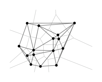
Figure 2: The Voronoi partition and the corresponding Delaunay graph

The coverage algorithm we consider is a distributed version of the classic Lloyd algorithm [14] based on “centering and partitioning” for the computation of centroidal Voronoi partitions. The algorithm is distributed in the sense that each robot determines its region of responsibility and its motion plan based upon communication with only some neighbors. Specifically, communications among the robots takes place along the edges of the Delaunay graph. The distributed coverage algorithm is described as follows. At each discrete time instant $t\in\mathbb{Z}_{\geq 0}$, each agent $i$ performs the following tasks: (i) it transmits its position and receives the positions of its neighbors in the Delaunay graph; (ii) it computes its Voronoi region with the information received; (iii) it moves to the centroid of its Voronoi region. In mathematical terms, for $t\in\mathbb{Z}_{\geq 0}$,

$$p(t+1)=\operatorname{Cd}(V(p(t))).$$ (8)

A variation of the function $\mathcal{H}_{\textup{multicenter}}$ is useful to analyze this algorithm. We define the positions-based multicenter function $\mathcal{H}_{\textup{Voronoi}}:Q^{N}\setminus S_{N}\rightarrow\mathbb{R}_{\geq 0}$ by

$$\mathcal{H}_{\textup{Voronoi}}(p) =\mathcal{H}_{\textup{multicenter}}(V(p),p)=\sum_{i=1}^{N}\int_{V_{i}(p)}f(\|q-p_{i}\|)\phi(q)dq.$$ (9)

Because of the compactness of $Q$, a continuity property, and the monotonicity properties in Proposition 2.4, one can show [9, Theorem 5.5] that $\mathcal{H}_{\textup{Voronoi}}$ is monotonically non-increasing along the solutions of (8) and that all solutions of (8) converge asymptotically to the set of configurations that generate centroidal Voronoi partitions. Additional considerations about convergence are given in [13].

3 Gossip coverage control as a dynamical system on the space of partitions

In this section we present the problem of interest, our novel gossip coverage algorithm and its convergence properties in Subsections 3.1, 3.2 and 3.3, respectively. In order to reduce the communication requirements of our algorithm, we propose an adjacency-based and continuous algorithm in Subsection 3.4. Finally, we report some simulation results in Subsection 3.5.

3.1 Problem statement

The distributed coverage law, based upon the Lloyd algorithm and described in the previous section, has some important limitations: it is applicable only to robotic networks with synchronized and reliable communication along all edges of the Delaunay graph (computed as a function of the robots’ positions). In other words, the law (8) requires that there exists a predetermined common communication schedule for all robots and, at each communication round, each robot must simultaneously and reliably communicate its position. Note that the Delaunay graph, interpreted as a communication graph, has the following drawbacks: for worst-case robots’ positions, a robot might have $N-1$ neighbors in the Delaunay graph and/or might have a neighbor that is arbitrarily far inside the environment. Therefore, each robot must be capable to communicate potentially to all other robots and/or to robots at large distances.

Given this broad range of undesirable limitations, the aim of this paper is to reduce the communication requirements of distributed coverage algorithms, in terms of reliability, synchronization and topology. Here are some relevant questions that constitute our informal problem statement:

Is it possible to optimize robots positions and environment partition with asynchronous, unreliable, and delayed communication? Specifically, what if the communication model is that of gossiping agents, that is, a model in which only a pair of robots can communicate at any time? Since Voronoi partitions generated by gossiping and moving agents cannot be computed by gossiping agents, how do we update the environment partition?

To answer these questions, the next subsections propose an innovative partition-based gossip approach, in which the robots’ positions essentially play no role and where instead dominance regions are iteratively updated. Designing coverage algorithms as dynamical systems on the space of partitions has the key advantage that one is not restricted to working only with Voronoi or anyway position-dependent partitions.

Example 3.1 (The Lloyd algorithm in the partition-based approach)

The distributed coverage algorithm (8) updates the robots’ positions so as to incrementally minimize the function $\mathcal{H}_{\textup{Voronoi}}$, while the environment partition is a function of the robots’ positions. In this paper we take a dual approach: we consider an algorithm that evolves partitions. From this partition-based viewpoint, the coverage algorithm is an iterated map on $\mathcal{V}_{N}$ and equation (8) is rewritten as $v(t+1)=V(\operatorname{Cd}(v(t)))$. $\square$

3.2 The gossip coverage algorithm

In this subsection we present a novel partition-based coverage algorithm in which, at each communication round, only two regions communicate. Recall the notion of bisector half-space from equation (3).

  Gossip Coverage Algorithm   For all $t\in\mathbb{Z}_{\geq 0}$, each agent $i\in\{1,\dots,N\}$ maintains in memory a dominance region $v_{i}(t)$. The collection $(v_{1}(0),\dots,v_{N}(0))$ is an arbitrary polygonal $N$-partition of $Q$. At each $t\in\mathbb{Z}_{\geq 0}$ a pair of communicating regions, say $v_{i}(t)$ and $v_{j}(t)$, is selected by a deterministic or stochastic process to be determined. Every agent $k\not\in\{i,j\}$ sets $v_{k}(t+1):=v_{k}(t)$. Agents $i$ and $j$ perform the following tasks:

1:  agent $i$ transmits to agent $j$ its dominance region $v_{i}(t)$ and vice-versa

2:  both agents compute the centroids $\operatorname{Cd}(v_{i}(t))$ and $\operatorname{Cd}(v_{j}(t))$

3:  if $\operatorname{Cd}(v_{i}(t))=\operatorname{Cd}(v_{j}(t))$ then

4:     $v_{i}(t+1):=v_{i}(t)$ and $v_{j}(t+1):=v_{j}(t)$

5:  else

6:     $v_{i}(t+1):=\big{(}v_{i}(t)\operatorname{\cup}v_{j}(t)\big{)}\operatorname{\cap}H_{\textup{bisector}}\big{(}\!\operatorname{Cd}(v_{i}(t));\operatorname{Cd}(v_{j}(t))\big{)}$ $v_{j}(t+1):=\big{(}v_{i}(t)\operatorname{\cup}v_{j}(t)\big{)}\operatorname{\cap}H_{\textup{bisector}}\big{(}\!\operatorname{Cd}(v_{j}(t));\operatorname{Cd}(v_{i}(t))\big{)}$

 

In other words, when two agents with distinct centroids communicate, their dominance regions evolve as follows: the union of the two dominance regions is divided into two new dominance regions by the hyperplane bisecting the segment between the two centroids; see Fig. 3. As a consequence, if the centroids $\operatorname{Cd}(v_{i}(t))$, $\operatorname{Cd}(v_{j}(t))$ are distinct, then $\{v_{i}(t+1),v_{j}(t+1)\}$ is the Voronoi partition of the set $v_{i}(t)\operatorname{\cup}v_{j}(t)$ generated by the centroids $\operatorname{Cd}(v_{i}(t))$ and $\operatorname{Cd}(v_{j}(t))$.

Figure 3: The gossip coverage algorithm. The left and right figure contain the initial partition and the partition after one application of the gossip coverage algorithm. In the middle figure we show the two centroids and (with a dashed line) the segment determining the bisector half-space.

We claim that the algorithm is well-posed in the sense that the sequence of collections $\{v(t)\}_{t\in\mathbb{Z}_{\geq 0}}$ generated by the algorithm is an $N$-partition at all times $t$. Indeed, it is immediate to see that the first two properties in Definition 2.1 are satisfied at all time if they are satisfied at initial time. Finally, at all times $t$, each component of $v(t)$ is clearly closed and has non-empty interior because of the following geometric fact: there exists no half-plane containing the interior of a region and not containing the centroid of the same region.

Now, for any $i,j\in\{1,\dots,N\}$ with $i\not=j$, define the map $T_{ij}:\mathcal{V}_{N}\rightarrow\mathcal{V}_{N}$ by

$$T_{ij}(v)=\begin{cases}v,&\text{if }\operatorname{Cd}(v_{i})=\operatorname{Cd}(v_{j}),\\ (v_{1},\dots,\widehat{v}_{i},\dots,\widehat{v}_{j},\dots,v_{N}),\quad&\text{otherwise},\end{cases}$$

where

$$\begin{split}\widehat{v}_{i}&=\big{(}v_{i}\operatorname{\cup}v_{j}\big{)}\operatorname{\cap}H_{\textup{bisector}}\big{(}\!\operatorname{Cd}(v_{i});\operatorname{Cd}(v_{j})\big{)},\\ \widehat{v}_{j}&=\big{(}v_{i}\operatorname{\cup}v_{j}\big{)}\operatorname{\cap}H_{\textup{bisector}}\big{(}\!\operatorname{Cd}(v_{j});\operatorname{Cd}(v_{i})\big{)}.\end{split}$$ (10)

The dynamical system on the space of partitions is therefore described by, for $t\in\mathbb{Z}_{\geq 0}$,

$$v(t+1)=T_{ij}(v(t)),$$ (11)

together with a rule describing what pair of regions $(i,j)$ is selected at each time. We also define the set-valued map $T:\mathcal{V}_{N}\rightrightarrows\mathcal{V}_{N}$ by $T(v)=\{T_{ij}(v)\,|\;i,j\in\{1,\dots,N\},\;i\neq j\}$. The map $T$ describes one iteration of the gossip coverage algorithm; an evolution of the gossip coverage algorithm is one of the solutions to the non-deterministic set-valued dynamical system $v(t+1)\in T(v(t))$.

Remark 3.2 (Gossip disk-covering control)

We believe that our gossip and partition-based algorithmic approach is applicable to a broad range of coverage problems. For example, the worst-case multicenter function [10] is defined by $\mathcal{H}_{\textup{worst}}(p,v)=\max_{i\in\{1,\dots,N\}}\max_{q\in{v_{i}}}\|q-p_{i}\|$. Maximizing $\mathcal{H}_{\textup{worst}}$ is equivalent to covering $Q$ with $N$ disks of smallest radius centered at $p$. As in Proposition 2.4, for any $v\in\mathcal{V}_{N}$ and $p\in Q^{N}\setminus S_{N}$, one can prove $\mathcal{H}_{\textup{worst}}(V(p),p)\leq\mathcal{H}_{\textup{worst}}(v,p)$ and $\mathcal{H}_{\textup{worst}}(v,\operatorname{CC}(v))\leq\mathcal{H}_{\textup{worst}}(v,p)$, where $\operatorname{CC}(v)$ is the array of circumcenters of the components of $v$. Hence, a gossip coverage algorithm for $\mathcal{H}_{\textup{worst}}$ is designed by replacing centroid with circumcenter operations in (10). We leave this and further extensions to future works. $\square$

3.3 Analysis results for the gossip coverage algorithm

In this subsection we state the main analysis and convergence results for the gossip coverage algorithm.

We begin by studying the fixed points of $T$ and by introducing an appropriate cost function with monotonicity properties along $T$. Regarding the algorithm’s fixed points, we extend Definition 2.5 as follows. A partition $v$ is mixed centroidal Voronoi if, for all pairs $(v_{i},v_{j})$ with $i\not=j$, either $\operatorname{Cd}(v_{i})=\operatorname{Cd}(v_{j})$ or $(v_{i},v_{j})$ is a centroidal Voronoi partition of $v_{i}\operatorname{\cup}v_{j}$, that is, $v_{i}=(v_{i}\operatorname{\cup}v_{j})\operatorname{\cap}H_{\textup{bisector}}\big{(}\!\operatorname{Cd}(v_{i});\operatorname{Cd}(v_{j})\big{)}$.

Lemma 3.3 (Fixed points of $T$ and centroidal Voronoi partitions)

For $i,j\in\{1,\dots,N\}$, $j\neq i$, denote the set of fixed points of $T_{ij}:\mathcal{V}_{N}\rightarrow\mathcal{V}_{N}$ by $F_{ij}=\{v\in\mathcal{V}_{N}\,|\;T_{ij}(v)=v\}$. The following statements hold:

1. $\operatorname{\cap}_{j\neq i}F_{ij}$ equals the set of mixed centroidal Voronoi partitions; and

2. if $v$ is a mixed centroidal Voronoi partition satisfying $\operatorname{Cd}(v_{i})\neq\operatorname{Cd}(v_{j})$ for $j\neq i$, then $v$ is centroidal Voronoi.

Next, we define the partition-based multicenter function $\mathcal{H}_{\textup{centroid}}:\mathcal{V}_{N}\rightarrow\mathbb{R}_{\geq 0}$ by

$$\mathcal{H}_{\textup{centroid}}(v) =\mathcal{H}_{\textup{multicenter}}(v,\operatorname{Cd}(v))=\sum_{i=1}^{N}\int_{v_{i}}f(\|q-\operatorname{Cd}(v_{i})\|)\phi(q)dq.$$ (12)

Lemma 3.4 (Monotonicity of $\mathcal{H}_{\textup{centroid}}$ along $T$)

For $i,j\in\{1,\dots,N\}$, $i\not=j$,

$$\mathcal{H}_{\textup{centroid}}(T_{ij}(v)) \leq\mathcal{H}_{\textup{centroid}}(v),\enspace \text{for all }v\in\mathcal{V}_{N},\text{ and}$$

$$\mathcal{H}_{\textup{centroid}}(T_{ij}(v)) <\mathcal{H}_{\textup{centroid}}(v), \text{iff $T_{ij}(v)$ and $v$ differ by a set of measure zero}.$$

The proofs of Lemmas 3.3 and 3.4 consist of elementary manipulations and are omitted in the interest of brevity. In short, we have established that the function $\mathcal{H}_{\textup{centroid}}$ monotonically decreases along each $T_{ij}$ when away from fixed points, and that centroidal Voronoi partitions are the fixed points of all $T_{ij}$ provided centroids are distinct.

We now prepare to state the main convergence result for $T$. We need to introduce some useful properties for sequences of partitions and for switching signals.

Definition 3.5 (Non-degeneracy)

A sequence of $N$-partitions $\{v(t)\}_{t\in\mathbb{Z}_{\geq 0}}$ is

1. (uniformly) distinct centroidal if there exists $\epsilon>0$ such that, for all $t\in\mathbb{Z}_{\geq 0}$ and $i,j\in\{1,\dots,N\}$, $i\not=j$, one has $\|\operatorname{Cd}(v_{i}(t))-\operatorname{Cd}(v_{j}(t))\|\geq\epsilon$;

2. (uniformly componentwise) non-vanishing if there exists $\epsilon>0$ such that, for all $t\in\mathbb{Z}_{\geq 0}$ and $i\in\{1,\dots,N\}$, the Lebesgue measure of $v_{i}(t)$ is greater than $\epsilon$; and

3. (uniformly componentwise) finitely convex if there exists $\ell\in{\mathbb{N}}$ such that, for all $t\in\mathbb{Z}_{\geq 0}$ and $i\in\{1,\dots,N\}$, the set $v_{i}(t)$ is the union of at most $\ell$ convex sets.

Moreover, the sequence $v$ is said to be non-degenerate if it is distinct centroidal, non-vanishing and finitely convex.

For example, a sequence of partitions is finitely-convex if each component of each partition in the sequence is the union of a uniformly bounded number of polygons with a uniformly bounded number of vertices.

Definition 3.6 (Uniform and random persistency)

Let $X$ be a finite set.

1. A map $\sigma:\mathbb{Z}_{\geq 0}\rightarrow X$ is uniformly persistent if there exists a duration $\Delta\in{\mathbb{N}}$ such that, for each $x\in{X}$, there exists an increasing sequence of times $\{t_{k}\}_{k\in\mathbb{Z}_{\geq 0}}\subset\mathbb{Z}_{\geq 0}$ satisfying $t_{k+1}-t_{k}\leq\Delta$ and $\sigma(t_{k})=x$ for all $k\in\mathbb{Z}_{\geq 0}$.

2. A stochastic process $\sigma:\mathbb{Z}_{\geq 0}\rightarrow X$ is randomly persistent if there exists a probability $p\in{]0,1[}$ and a duration $\Delta\in{\mathbb{N}}$ such that, for each $x\in{X}$ and for each $t\in\mathbb{Z}_{\geq 0}$, there exists $k\in\{1,\dots,\Delta\}$ satisfying

   $$\mathbb{P}\big{[}\sigma(t+k)=x\,|\,\sigma(t),\dots,\sigma(1)\big{]}\geq p.$$

We are now ready to state the main deterministic and stochastic convergence results for the gossip coverage algorithm. It is convenient to postpone to Section 6.2 the theorem proof and the definition of convergence in the space of partitions.

Theorem 3.7 (Convergence under persistent gossip)

Consider the gossip coverage algorithm $T$ and the evolutions $\{v(t)\}_{t\in\mathbb{Z}_{\geq 0}}\subset\mathcal{V}_{N}$ defined by

$$v(t+1)=T_{\sigma(t)}(v(t)),\quad\text{for }t\in\mathbb{Z}_{\geq 0},$$

where $\sigma:\mathbb{Z}_{\geq 0}\rightarrow\{(i,j)\in\{1,\dots,N\}^{2}\,|\;i\not=j\}$ is either a deterministic map or a stochastic process. Then the following statements hold:

1. if $\sigma$ is a uniformly persistent map, then each non-degenerate evolution $v$ converges to the set of centroidal Voronoi partitions; and

2. if $\sigma$ is a randomly persistent stochastic process, then each evolution $v$, conditioned upon being non-degenerate, converges almost surely to the set of centroidal Voronoi partitions.

The statements of Theorem 3.7 rely upon the assumption of non-degenerate evolutions. It is our conjecture that, starting from generic polygonal partition, this assumption is typically satisfied. We will discuss some numerical evidence to this effect in the next section.

Lemma 3.4 indicates how the function $\mathcal{H}_{\textup{centroid}}$ plays the role of a Lyapunov function for the dynamical system defined by $T$. To provide a complete Lyapunov convergence proof of Theorem 3.7, we set out to establish three sets of relevant results. First, we need to establish extensions of the Krasovskii-LaSalle invariance principle for set-valued dynamical systems over compact metric spaces. Second, we need to establish the compactness properties of the space of non-degenerate partitions. Third, we need to establish the continuity of the relevant geometric maps. These three topics are the subjects of Section 4, 5 and 6, respectively.

3.4 Designing an adjacency-based and continuous algorithm

The gossip coverage map $T$ has the undesirable feature that it entails communication exchanges between any two regions. This communication requirement might be too onerous in some multiagent applications. Ideally we would like to require communications only between adjacent regions, that is, regions whose boundaries touch, or between “nearby” regions. We believe such communication requirements may be easily achieved in robotic networks and we detail a sample implementation for robots with range-dependent Poisson communication in Appendix A. Additionally, we aim to design a continuous gossip coverage map. We require the modified map to be continuous for technical reasons: the invariance principles we adopt for the convergence analysis require continuity of the dynamical system.

Motivated by this discussion, we modify the map $T$ to rely upon only adjacency-based communication and to be continuous. First, we introduce a pseudodistance notion between sets. Given closed $A\subset{Q}$ and $B\subset{Q}$ with non-empty interior, define

$$\operatorname{pseudodist}(A,B)=\inf\{\|a-b\|\,|\;(a,b)\in\operatorname{int}(A)\times\operatorname{int}(B)\}.$$

Second, we select a positive constant $\delta\ll\operatorname{diam}(Q)$ and denote by $T^{\delta}:\mathcal{V}_{N}\rightarrow\mathcal{V}_{N}$ the modified gossip coverage map to be defined in what follows. For any $i,j\in\{1,\dots,N\}$, $i\neq{j}$, we give the following partial definition:

$$T^{\delta}_{ij}(v)=\begin{cases}v,&\text{if }\big{(}\|\operatorname{Cd}(v_{i})-\operatorname{Cd}(v_{j})\|=0\big{)}\text{ or\phantom{and} }\big{(}\operatorname{pseudodist}(v_{i},v_{j})\geq\delta\big{)},\\ T(v),&\text{if }\big{(}\|\operatorname{Cd}(v_{i})-\operatorname{Cd}(v_{j})\|\geq\delta\big{)}\text{ and\phantom{or} }\big{(}\operatorname{pseudodist}(v_{i},v_{j})=0\big{)}.\end{cases}$$ (13)

Therefore, if either $\operatorname{Cd}(v_{i})$ and $\operatorname{Cd}(v_{j})$ coincide or the pseudodistance between $v_{i}$ and $v_{j}$ is larger than $\delta$, then $T^{\delta}_{ij}(v)=v$, that is, the map $T^{\delta}_{ij}$ leaves the partition unchanged. Additionally, if the pseudodistance between the regions $v_{i}$ and $v_{j}$ is zero ($v_{i}$ and $v_{j}$ are adjacent) and the distance between $\operatorname{Cd}(v_{i})$ and $\operatorname{Cd}(v_{j})$ is larger than $\delta$, then $T^{\delta}_{ij}(v)=T_{ij}(v)$.

Next, we consider partitions that do not satisfy either of the two conditions in definition (13). We define the unit saturation function $\operatorname{sat}:\mathbb{R}_{\geq 0}\rightarrow[0,1]$ by $\operatorname{sat}(x)=x$ if $x\in[0,1]$, and $\operatorname{sat}(x)=1$ if $x>1$ and the scaling function $\beta_{ij}:\mathcal{V}_{N}\rightarrow[0,1]$ by

$$\beta_{ij}(v)=\operatorname{sat}\!\big{(}\|\operatorname{Cd}(v_{i})-\operatorname{Cd}(v_{j})\|/\delta\big{)}\Big{(}1-\operatorname{sat}\!\big{(}\operatorname{pseudodist}(v_{i},v_{j})/\delta\big{)}\Big{)}.$$

The first condition and the second condition in (13) correspond precisely to $\beta_{ij}(v)=0$ and $\beta_{ij}(v)=1$, respectively. For partitions $v$ satisfying $0<\beta_{ij}(v)<1$, we aim to define $T^{\delta}$ so as to continuously interpolate between the identity map and the map $T$; see Fig. 4 for an illustration.

Figure 4: Modified gossip between close but not adjacent regions ($0<\beta_{12}(v)<1$). The bisecting line $\gamma_{\perp}$ borders the set $R_{2}=v_{2}\operatorname{\cap}H_{\textup{bisector}}(\operatorname{Cd}(v_{1}),\operatorname{Cd}(v_{2}))$ that, in the map $T$, is assigned to $v_{1}$ (see Fig. 3). According to $T^{\delta}$ instead, only the subset $\widehat{R}_{2}\subsetneq R_{2}$ is assigned to $v_{1}$. Loosely speaking, the “width” of $\widehat{R}_{2}$ equals $\beta_{12}(v)$ times the “width” of $R_{2}$, where “width” of a set is the maximum distance from a point in the set to $\gamma_{\perp}$.

Let $R_{i}=v_{i}\operatorname{\cap}H_{\textup{bisector}}(\operatorname{Cd}(v_{j}),\operatorname{Cd}(v_{i}))$ and $R_{j}=v_{j}\operatorname{\cap}H_{\textup{bisector}}(\operatorname{Cd}(v_{i}),\operatorname{Cd}(v_{j}))$. Define the line $\gamma_{\perp}=\partial H_{\textup{bisector}}(\operatorname{Cd}(v_{j}),\operatorname{Cd}(v_{i}))$ and

$$\begin{split}\widehat{p}_{i}&=\text{a point in }\overline{\operatorname{int}{(R_{i})}}\text{ that is maximally distant from }\gamma_{\perp},\\ \widehat{p}_{j}&=\text{a point in }\overline{\operatorname{int}{(R_{j})}}\text{ that is maximally distant from }\gamma_{\perp}.\end{split}$$ (14)

Next, note that for each $q\in{R_{i}\cup{R_{j}}}$ there exists a unique line, say $\gamma_{q}$, that is parallel to $\gamma_{\perp}$ and passes through $q$. Based on this notion, we define

$$\widehat{R}_{i} =\{q\in R_{i}\,|\;\operatorname{dist}(\widehat{p}_{i},\gamma_{q})\leq\beta_{ij}(v)\operatorname{dist}(\widehat{p}_{i},\gamma_{\perp})\,\,\,\text{or}\,\,\,\operatorname{dist}(q,\gamma_{\perp})\geq\operatorname{dist}(\widehat{p}_{i},\gamma_{\perp})\},$$

$$\widehat{R}_{j} =\{q\in R_{j}\,|\;\operatorname{dist}(\widehat{p}_{j},\gamma_{q})\leq\beta_{ij}(v)\operatorname{dist}(\widehat{p}_{j},\gamma_{\perp})\,\,\,\text{or}\,\,\,\operatorname{dist}(q,\gamma_{\perp})\geq\operatorname{dist}(\widehat{p}_{j},\gamma_{\perp})\}.$$

We can now complete the partial definition (13). For all $v$ with $0<\beta_{ij}(v)<1$, that is, for all partitions not already dealt with in definition (13), we define

$$T^{\delta}_{ij}(v)=(v_{1},\dots,\underbrace{\overline{\big{(}v_{i}\setminus\widehat{R}_{i}\big{)}\cup\widehat{R}_{j}}}_{i\text{th entry}},\dots,\underbrace{\overline{\big{(}v_{j}\setminus\widehat{R}_{j}\big{)}\cup\widehat{R}_{i}}}_{j\text{th entry}},\dots,v_{N}).$$

As discussed for $T$, one can prove that the map $T^{\delta}:\mathcal{V}_{N}\rightrightarrows\mathcal{V}_{N}$ defined by $T^{\delta}(v)=\{T^{\delta}_{ij}(v)\,|\;i,j\in\{1,\dots,N\},\,i\neq j\}$, is well-posed and has the following properties.

Theorem 3.8 (Convergence of modified gossip map)

Consider the modified gossip coverage algorithm $T^{\delta}$ and the evolutions $\{v(t)\}_{t\in\mathbb{Z}_{\geq 0}}\subset\mathcal{V}_{N}$ defined by

$$v(t+1)=T^{\delta}_{\sigma(t)}(v(t)),\quad\text{for }t\in\mathbb{Z}_{\geq 0},$$

where $\sigma:\mathbb{Z}_{\geq 0}\rightarrow\{(i,j)\in\{1,\dots,N\}^{2}\,|\;i\not=j\}$ is either a deterministic map or a stochastic process. Then the following statements hold:

1. if $\sigma$ is a uniformly persistent map, then each non-vanishing and finitely-convex evolution $v$ converges to the set of mixed centroidal Voronoi partitions; and

2. if $\sigma$ is a randomly persistent stochastic process, then each evolution $v$, conditioned upon being non-vanishing and finitely convex, converges almost surely to the set of mixed centroidal Voronoi partitions.

3.5 Simulation results and implementation remarks

We have extensively simulated the partition-based gossip coverage algorithm $T$ on a $2$-dimensional polygonal environment with uniform density and performance function $f(x)=x^{2}$. Simulations have been implemented as a Matlab program, using the General Polygon Clipper Library to perform operations on polygons. We adopted the following communication model: at each iteration, a region pair is chosen, uniformly at random, among all pairs of adjacent regions. Fig. 5 is an illustration of a typical evolution.

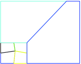
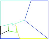
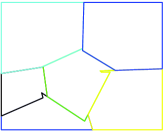
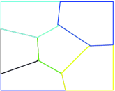
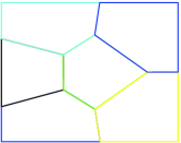
Figure 5: An example simulation of the gossip coverage algorithm with uniform random edge selection. The environment $Q$ is a rectangle with uniform density, centroids are computed with performance function $f(x)=x^{2}$, and $N=6$ regions compose the partition. Snapshots of an evolution are shown for $t\in\{0,20,50,100,300\}$. One may verify numerically that the sequence converges asymptotically to a centroidal Voronoi partition. At $t=20$ one of the regions is disconnected.

Our first numerical finding is that the gossip coverage algorithm appears to converge to centroidal Voronoi partitions from all initial conditions. This is the same property that the Lloyd synchronous coverage algorithm (8) is known to possess. In other words, our numerically-computed sequences of partitions always converge to centroidal Voronoi partitions – even though our theoretical analysis (1) requires a continuous interpolation from $T$ to $T^{\delta}$ and (2) does not exclude convergence to degenerate partitions where some component regions might have coincident centroids, or might have empty interiors, or might be composed of “polygons with an infinite number of vertices,” that is, arbitrary sets.

A second numerical finding is that, throughout numerous sample executions, the resulting polygonal regions rarely have complicated shapes and large numbers of vertices. This is good news because of our assumption of finite convexity and because large numbers of vertices affect both the computation and the communication burden of the gossip coverage algorithm.

Finally, it is possible, and we have observed it numerically, to have evolutions of the algorithm that, before converging to centroidal Voronoi partitions, have components with disconnected regions. We believe that there might be applications where it is desirable to maintain connectivity of the components of the partition and, therefore, we sketch here how to design a connectivity-preserving algorithm. Note that the update step of the partition-based coverage algorithm amounts to the exchange, among the agents, of a region, which consists in general of several connected components. In the connectivity-preserving algorithm, such components are considered individually, and each of them is traded only if this can be done without loosing connectivity; if not, the component is kept by the previous owner. Numerical simulations indicate that such an algorithm leads to centroidal Voronoi partitions as well.

4 On the Krasovskii–LaSalle invariance principle: set-valued maps on metric spaces

In this section we consider discrete-time set-valued dynamical system defined on metric spaces. Our goal is to provide some extensions of the classical Krasovskii-LaSalle Invariance Principle; we refer the interested reader to [5, 20, 34] for recent invariance principles for switched continuous-time and hybrid systems.

We start by reviewing some preliminary notions including set-valued dynamical systems, continuity and invariance properties, and Lyapunov functions. On a metric space $(X,d)$, where $X$ is a set and $d$ is a metric on $X$, a set-valued map $T:X\rightrightarrows X$ is non-empty if $T(x)\neq\emptyset$ for all $x\in{X}$. An evolution of the dynamical system determined by a non-empty set-valued map $T$ is a sequence $\{x_{n}\}_{n\in\mathbb{Z}_{\geq 0}}\subset X$ with the property that

$$x_{n+1}\in T(x_{n}),\quad n\in\mathbb{Z}_{\geq 0}.$$

In other words, we regard a set-valued map as a nondeterministic discrete-time dynamical system. For set-valued maps we introduce notions of continuity and invariance as follows. A set-valued map $T$ is closed at $x\in{X}$ if, for all pairs of convergent sequences $x_{k}\to x$ and $x^{\prime}_{k}\to x^{\prime}$ such that $x^{\prime}_{k}\in T(x_{k})$, one has that $x^{\prime}\in T(x)$. Additionally, $T$ is closed on $W\subset X$ if it is closed at all $w\in{W}$. A set $W\subset{X}$ is weakly positively invariant for $T$ if $T(w)\operatorname{\cap}{W}$ is non-empty for all $w\in{W}$. A set $W$ is strongly positively invariant for $T$ if $T(w)\subset{W}$ for all $w\in{W}$.

We are ready now to state a Krasovskii-LaSalle invariance principle for set-valued maps defined on metric spaces. This result extends the Global Convergence Theorem in [26] to more general Lyapunov functions. Its proof follows the lines of the proof of Theorem 1.21 in [9], and is thus omitted.

Lemma 4.1 (Krasovskii-LaSalle invariance principle for set-valued maps)

Let $(X,d)$ be a metric space and $T:X\rightrightarrows X$ be non-empty. Assume that:

1. there exists a compact set $W\subseteq X$ that is strongly positively invariant for $T$;

2. there exists a function $U:W\rightarrow\mathbb{R}$ such that $U(w^{\prime})\leq U(w)$, for all $w\in W$ and $w^{\prime}\in T(w)$;

3. the function $U$ is continuous on $W$ and the map $T$ is closed on $W$.

Then there exists $c\in\mathbb{R}$ such that each evolution of $T$ with initial condition in $W$ approaches a set of the form $S\operatorname{\cap}U^{-1}(c)$, where $S$ is the largest weakly positively invariant set contained in

$$\{w\in{W}\,|\;\exists\,w^{\prime}\in T(w)\;\text{such that}\;U(w^{\prime})=U(w)\}.$$

In this paper, given the metric space $(X,d)$, we deal with a set-valued map $T:X\rightrightarrows X$ defined by a collection of maps $T_{1},\ldots,T_{m}:X\rightarrow X$ via the equality $T(x)=\left\{T_{1}(x),\ldots,T_{m}(x)\right\}$ for $x\in X$. For this kind of set-valued maps, closedness is related to continuity of ordinary maps.

Lemma 4.2

Let $T_{1},\ldots,T_{m}:X\rightarrow X$ be continuous on $W\subset{X}$. The set-valued map $T:X\rightrightarrows X$ defined by $T(x)=\left\{T_{1}(x),\ldots,T_{m}(x)\right\}$ is closed on $W$.

Proof.   Let $w_{n}\to w$ and $w^{\prime}_{n}\to w^{\prime}$ be a pair of convergent sequences in $W$, such that $w^{\prime}_{n}\in T(w_{n})$. We claim that the continuity of $T_{1},\ldots,T_{m}$ implies $w^{\prime}\in T(w)$.

Note that, by hypothesis, for all $n\in\mathbb{Z}_{\geq 0}$ there exists $i_{n}\in\left\{1,\ldots,m\right\}$ such that $w^{\prime}_{n}=T_{i_{n}}(w_{n})$. Because the set $\left\{1,\ldots,m\right\}$ is finite, there exists an index $j\in\left\{1,\ldots,m\right\}$ that appears infinitely many times in the sequence $\{i_{n}\}_{n\in{\mathbb{N}}}$. Consider the subsequences $\{w_{n_{l}}\}\subseteq\{w_{n}\}$ and $\{w^{\prime}_{n_{l}}\}\subseteq\{w^{\prime}_{n}\}$, such that $w^{\prime}_{n_{l}}=T_{j}(w_{n_{l}})$. Clearly, we have that $w_{n_{l}}\to w$ and $w^{\prime}_{n_{l}}\to w^{\prime}$, where from the continuity of $T_{j}$ it follows that $w^{\prime}=T_{j}(w)$. Thus, $w^{\prime}\in T(w)$ and the claim is proved.  

The following result is a stronger version of Lemma 4.1, for a particular class of set-valued dynamical systems.

Theorem 4.3 (Uniformly persistent switches imply convergence)

Let $(X,d)$ be a metric space. Given a collection of maps $T_{1},\ldots,T_{m}:X\rightarrow X$, define the set-valued map $T:X\rightrightarrows X$ by $T(x)=\left\{T_{1}(x),\ldots,T_{m}(x)\right\}$ and let $\{x_{n}\}_{n\in\mathbb{Z}_{\geq 0}}$ be an evolution of $T$. Assume that:

1. there exists a compact set $W\subseteq X$ that is strongly positively invariant for $T$;

2. there exists a function $U:W\rightarrow\mathbb{R}$ such that $U(w^{\prime})<U(w)$, for all $w\in W$ and $w^{\prime}\in T(w)\setminus\{w\}$;

3. the maps $T_{i}$, for $i\in\{1,\dots,m\}$, and $U$ are continuous on $W$; and

4. for all $i\in\{1,\dots,m\}$, there exists an increasing sequence of times $\{n_{k}\,|\;k\in\mathbb{Z}_{\geq 0}\}$ such that $x_{n_{k}+1}=T_{i}(x_{n_{k}})$ and $(n_{k+1}-n_{k})$ is bounded.

If $x_{0}\in{W}$, there exists $c\in\mathbb{R}$ such that the evolution $\{x_{n}\}_{n\in\mathbb{Z}_{\geq 0}}$ approaches the set

$$(F_{1}\operatorname{\cap}\cdots\operatorname{\cap}F_{m})\operatorname{\cap}U^{-1}(c),$$

where $F_{i}=\{w\in W\,|\;T_{i}(w)=w\}$ is the set of fixed points of $T_{i}$ in $W$, $i\in\{1,\dots,m\}$.

Loosely speaking, (i) the compactness of a strongly positively invariant set, (ii) a monotonicity property for a Lyapunov function, (iii) continuity properties, and (iv) uniformly persistent switches among finitely many maps, together ensure convergence of each evolution to the intersection of the fixed points of the maps.

Proof.  [Proof of Theorem 4.3] Let $S$ be the largest weakly positively invariant set contained in

$$\{w\in W\,|\;\exists\,w^{\prime}\in T(w)\text{ such that }U(w^{\prime})=U(w)\}=F_{1}\operatorname{\cup}\cdots\operatorname{\cup}F_{m}.$$

Since $T$ is closed by Lemma 4.2, the assumptions of Lemma 4.1 are met; hence there exists $c\in\mathbb{R}$ such that $U(x_{n})\to c$ and $x_{n}\to S\operatorname{\cap}U^{-1}(c)$.

Let $\Omega(x_{n})$ denote the $\omega$-limit set of the sequence $\{x_{n}\,|\;n\in\mathbb{Z}_{\geq 0}\}$. If we show that $\Omega(x_{n})\subseteq(F_{1}\operatorname{\cap}\cdots\operatorname{\cap}F_{m})\operatorname{\cap}U^{-1}(c)$, then the statement of the theorem is proved. We proceed by contradiction. To this aim, let $\widehat{x}\in S\operatorname{\cap}U^{-1}(c)\setminus\big{(}(F_{1}\operatorname{\cap}\cdots\operatorname{\cap}F_{m})\operatorname{\cap}U^{-1}(c)\big{)}$ and let $\{x_{n_{h}}\}_{h\in\mathbb{Z}_{\geq 0}}$ be a subsequence such that $x_{n_{h}}\to\widehat{x}$.

Observe that for each $\widehat{x}\in S\setminus(F_{1}\operatorname{\cap}\cdots\operatorname{\cap}F_{m})$, there exists a non-empty set $\mathcal{I}_{\widehat{x}}\subset\left\{1,\ldots,m\right\}$ such that, $\widehat{x}=T_{i}\left(\widehat{x}\right)$ if $i\in\mathcal{I}_{\widehat{x}}$, and $\widehat{x}\neq T_{i}\left(\widehat{x}\right)$ if $i\notin\mathcal{I}_{\widehat{x}}$. By the continuity of the maps $T_{i}$, there exists $\delta\in\mathbb{R}_{>0}$ such that, if $i\notin\mathcal{I}_{\widehat{x}}$, then $T_{i}(x)\neq x$ for all $x\in B_{\delta}(\widehat{x})=\{x\in{W}\,|\;d(x,\widehat{x})\leq\delta\}$. Let now

$$\gamma_{\delta}=\min_{i\in\mathcal{I}_{\widehat{x}}}\left\{\min_{x\in B_{\delta}(\widehat{x})}\Big{(}U\left(x\right)-U\left(T_{i}(x)\right)\Big{)}\right\}\geq 0.$$

By hypothesis, if $i\notin\mathcal{I}_{\widehat{x}}$, then $U(T_{i}(x))<U(x)$ for all $x\in B_{\delta}(\widehat{x})$. Hence, since $B_{\delta}(\widehat{x})$ is closed, and $U$ and the maps $T_{i}$ are continuous, we deduce that $\gamma>0$.

Observe now that hypothesis (iv) implies the existence of a duration $D\in{\mathbb{N}}$ such that every map $T_{i}$, $i\in\{1,\dots,m\}$, is applied at least once within every interval ${[n,n+D[}$, for all $n\in\mathbb{Z}_{\geq 0}$. Consider the set $\left\{T_{i}\right\}_{i\in\mathcal{I}_{\widehat{x}}}$; this is a collection of continuous maps having $\widehat{x}$ as fixed point. Then, there exists a suitable $\epsilon\in\mathbb{R}_{>0}$ such that, given any $r$-uple $(j_{1},\ldots,j_{r})\in\mathcal{I}_{\widehat{x}}^{r}$, $r\leq D$, we have that $T_{j_{1}}\circ T_{j_{2}}\circ T_{j_{3}}\circ\ldots\circ T_{j_{r}}(x)\in B_{\delta}(\widehat{x})$ for all $w\in B_{\epsilon}(\widehat{x})$.

Select now $k$ such that the element $x_{n_{k}}$ in the subsequence $\{x_{n_{h}}\}_{h\in\mathbb{Z}_{\geq 0}}$ satisfies $d\left(x_{n_{k}},\widehat{x}\right)<\epsilon$ and ${U(x_{n_{k}})-c<\gamma_{\delta}}$. Let

$$s=\min\{t\in[1,D[\,|\;\exists\,j\notin\mathcal{I}_{\widehat{x}}\text{ such that }x_{n_{k}+t+1}=T_{j}\left(x_{n_{k}+t}\right)\}.$$

Observe that $U(x_{n_{k}+s})-c<\gamma_{\delta}$ and $U(x_{n_{k}+s})-U\big{(}T_{j}(x_{n_{k}+s})\big{)}\geq\gamma_{\delta}$ implying that $U\left(T_{j}\left(x_{n_{k}+s}\right)\right)<c$. This is a contradiction.  

Remark 4.4

An alternate proof of this theorem can be given by applying an invariance principle obtained in [34] on an appropriately-designed dynamical extension of the discrete-time set-valued system. $\square$

In Appendix B we show how to persistent switching assumption is necessary. Next, we provide a probabilistic version of the previous theorem.

Theorem 4.5 (Persistent random switches imply convergence)

Let $(X,d)$ be a metric space. Given a collection of maps $T_{1},\ldots,T_{m}:X\rightarrow X$, define the set-valued map $T:X\rightrightarrows X$ by $T(x)=\left\{T_{1}(x),\ldots,T_{m}(x)\right\}$. Given a stochastic process $\sigma:\mathbb{Z}_{\geq 0}\rightarrow\{1,\dots,m\}$, consider an evolution $\{x_{n}\}_{n\in\mathbb{Z}_{\geq 0}}$ of $T$ satisfying

$$x_{n+1}=T_{\sigma(n)}(x_{n}).$$

Assume that:

1. there exists a compact set $W\subseteq X$ that is strongly positively invariant for $T$;

2. there exists a function $U:W\rightarrow\mathbb{R}$ such that $U(w^{\prime})<U(w)$, for all $w\in W$ and $w^{\prime}\in T(w)\setminus\{w\}$;

3. the maps $T_{i}$, for $i\in\{1,\dots,m\}$, and $U$ are continuous on $W$; and

4. there exists $p\in{]0,1[}$ and $k\in{\mathbb{N}}$ such that, for all $i\in\{1,\dots,m\}$ and $n\in\mathbb{Z}_{\geq 0}$, there exists $h\in\{1,\dots,k\}$ such that

   $$\mathbb{P}\big{[}\sigma(n+h)=i\,|\,\sigma(n),\dots,\sigma(1)\big{]}\geq p.$$

If $x_{0}\in{W}$, then there exists $c\in\mathbb{R}$ such that almost surely the evolution $\{x_{n}\}_{n\in\mathbb{Z}_{\geq 0}}$ approaches the set

$$(F_{1}\operatorname{\cap}\cdots\operatorname{\cap}F_{m})\operatorname{\cap}U^{-1}(c),$$

where $F_{i}=\{w\in W\,|\;T_{i}(w)=w\}$ is the set of fixed points of $T_{i}$ in $W$, $i\in\{1,\dots,m\}$.

Loosely speaking, (i) the compactness of a strongly positively invariant set, (ii) a monotonicity property for a Lyapunov function, (iii) continuity properties, and (iv) persistent random switches among finitely many maps, together ensure convergence of each evolution to the intersection of the fixed points of the maps.

Proof.  [Proof of Theorem 4.5] If $x_{0}\in W$, then the stochastic process $\sigma$ induces a stochastic process taking values in $W$. From now on, we restrict our attention to sequences $\{x_{n}\}_{n\in\mathbb{Z}_{\geq 0}}$ such that $x_{0}\in W$. In other words we assume that the sample space containing all the evolutions of our interest is given by

$$\mathcal{A}=\big{\{}\{x_{n}\}_{n\in\mathbb{Z}_{\geq 0}}\,|\;x_{n}\in W\text{ for all }n\in\mathbb{Z}_{\geq 0}\big{\}}.$$

Let $S$ be the largest weakly positively invariant set contained in

$$\{w\in W\,|\;\exists\,w^{\prime}\in T(w)\text{ such that }U(w^{\prime})=U(w)\}=F_{1}\operatorname{\cup}\cdots\operatorname{\cup}F_{m}.$$

From Lemma 4.1, we know that there exists $c\in\mathbb{R}$ such that $x_{n}\to S\operatorname{\cap}U^{-1}(c)$. This implies that the following event is certain:

$$E=\big{\{}\{x_{n}\}_{n\in\mathbb{Z}_{\geq 0}}\,|\;\exists\,c\in\mathbb{R}\text{ such that }\lim_{n\to\infty}U(x_{n})=c\big{\}}.$$

Let $\Omega(x_{n})$ denote the $\omega$-limit set of the sequence $\{x_{n}\,|\;n\in\mathbb{Z}_{\geq 0}\}$. If we show that $\Omega(x_{n})\subseteq\left((F_{1}\operatorname{\cap}\cdots\operatorname{\cap}F_{m})\operatorname{\cap}U^{-1}(c)\right)$ almost surely, then the statement of the theorem is proved. Next, consider the event

$$E_{1}=\big{\{}\{x_{n}\}_{n\in\mathbb{Z}_{\geq 0}}\,|\;\exists\,\widehat{x}\in S\setminus(F_{1}\operatorname{\cap}\ldots\operatorname{\cap}F_{m})\text{ such that }\widehat{x}\in\Omega\left(x_{n}\right)\big{\}}.$$

Assume by contradiction that $\mathbb{P}\left[E_{1}\right]>0$. Now we compute $\mathbb{P}\left[E|E_{1}\right]$. Note that, for each $\widehat{x}\in S\setminus(F_{1}\operatorname{\cap}\ldots\operatorname{\cap}F_{m})$, there exists a non-empty set $\mathcal{I}_{\widehat{x}}\subset\{1,\dots,m\}$ such that, $\widehat{x}=T_{i}\left(\widehat{x}\right)$ if $i\in\mathcal{I}_{\widehat{x}}$, and $\widehat{x}\neq T_{i}\left(\widehat{x}\right)$ if $i\notin\mathcal{I}_{\widehat{x}}$. Similarly to the proof of Theorem 4.3, we can associate to each $\widehat{x}$ a positive real number $\delta$ such that the inequality $x\neq T_{i}\left(x\right)$ holds true for all $x\in B_{\delta}(\widehat{x})=\{x\in W\,|\;d(x,\widehat{x})\leq\delta\}$ and for all $i\notin\mathcal{I}_{\widehat{x}}$. Moreover, we can define

$$\gamma_{\delta}=\min_{i\in\mathcal{I}_{\widehat{x}}}\left\{\min_{x\in B_{\delta}(\widehat{x})}\Big{(}U(x)-U(T_{i}(x))\Big{)}\right\},$$

where the continuity of the maps $T_{j}$, $j\in\{1,\dots,m\}$, and $U$, and the closedness of the set $B_{\delta}(\widehat{x})$ ensure that $\gamma_{\delta}>0$.

Consider the set $\left\{T_{i}\right\}_{i\in\mathcal{I}_{\widehat{x}}}$; this is a collection of continuous maps having $\widehat{x}$ as fixed point. Therefore, there exists a suitable $\epsilon\in\mathbb{R}_{>0}$ such that, given any $r$-uple $(j_{1},\ldots,j_{r})\in\mathcal{I}_{\widehat{x}}^{r}$, $r\leq k$, we have $T_{j_{1}}\circ T_{j_{2}}\circ T_{j_{3}}\circ\ldots\circ T_{j_{r}}(x)\in B_{\delta}(\widehat{x})$ for all $x\in B_{\epsilon}(\widehat{x})$. Given $\{x_{n}\}_{n\in\mathbb{Z}_{\geq 0}}$, if there exists $\widehat{x}\in S\setminus(F_{1}\operatorname{\cap}\ldots\operatorname{\cap}F_{m})$ such that $\widehat{x}\in\Omega\left(x_{n}\right)$, then there must exist $\{n_{h}|\;h\in\mathbb{Z}_{\geq 0}\}$ such that $x_{n_{h}}\in B_{\epsilon}(\hat{x})$ for all $h\in\mathbb{Z}_{\geq 0}$. Moreover, without loss of generality we can assume that $n_{h+1}-n_{h}>k$ for all $h\in\mathbb{Z}_{\geq 0}$. Consider now the event

$$E_{3}=\big{\{}\{i_{n}\in\{1,\dots,m\}\,|\;n\in\mathbb{Z}_{\geq 0}\}\;|\\ \exists\,\bar{h}\text{ such that }i_{n_{h}+s}\in I_{\widehat{x}}\text{ for all }s\in\{1,\dots,k\}\text{ and }h\geq\bar{h}\big{\}}.$$

To compute $\mathbb{P}[E_{3}]$, we define, for $j\in\mathbb{Z}_{\geq 0}$,

$$E_{3,j}=\big{\{}\{i_{n}\in\{1,\dots,m\}\,|\;n\in\mathbb{Z}_{\geq 0}\}\,|\;i_{n_{h}+s}\in I_{\widehat{x}}\text{ for all }s\in\{1,\dots,k\}\text{ and }h\geq j\big{\}}.$$

Observe that $\{E_{3,j}\,|\;j\in\mathbb{Z}_{\geq 0}\}$ is a countable collection of disjoint sets such that $E_{3}=\bigcup_{j=0}^{\infty}E_{3,j}$. By hypothesis we have that

$$\mathbb{P}[E_{3,j}]\leq\lim_{l\to\infty}\prod_{s=j}^{l}(1-p)=0,$$

and therefore $\mathbb{P}[E_{3}]=0$. This implies that, almost surely, there exists a subsequence $\{n_{h_{s}}\}_{s\in\mathbb{Z}_{\geq 0}}\subseteq\{n_{h}\}_{h\in\mathbb{Z}_{\geq 0}}$ with the property that, for all $s\in\mathbb{Z}_{\geq 0}$, $x_{n_{h_{s}}+1}=T_{i}(x_{n_{h_{s}}})$ for some $i\notin\mathcal{I}_{\widehat{x}}$ and, therefore, also with the property that $U(x_{n_{h_{s}}})-U(x_{n_{h_{k}}+1})>\gamma_{\delta}$. Consequently, almost surely, we have that $\lim_{s\to\infty}U(x_{n_{h_{s}}})=-\infty$ thus violating the fact that $E$ is a certain event. This implies that $\mathbb{P}\left[E_{1}\right]=0$ and that, almost surely, $x_{n}\to(F_{1}\operatorname{\cap}\ldots\operatorname{\cap}F_{m})\operatorname{\cap}U^{-1}(c)$.  

Remark 4.6

The assumption, in Lemma 4.1 and Theorems 4.3 and 4.5, that $W$ is strongly positively invariant ensures that any evolution of $T$ with initial condition in $W$ remains in $W$. By relaxing this assumption, it is possible to provide weaker versions of these results. Specifically, requiring $W$ to be only compact and not necessarily strongly positively invariant, the thesis of Lemma 4.1 and Theorems 4.3 and 4.5 do not hold in general for any evolution of $T$ with initial condition on $W$, but are still valid for those evolutions $\{x_{n}\}_{n\in\mathbb{Z}_{\geq 0}}$ that take values in $W$ for all $n\in\mathbb{Z}_{\geq 0}$. $\square$

5 On the topology of the space of partitions: compactness properties in the symmetric difference metric

Motivated by the invariance principles presented in Section 4, we study metric structures on the set of partitions, with a focus on compactness and continuity properties. Specifically, we show how a particular subset of the set of partitions can be regarded as a compact metric space and how certain relevant maps are continuous over that subspace. In this section, and only in this section, the assumptions on $Q$ are relaxed to give more general results: we assume that $Q\subset\mathbb{R}^{d}$ is compact and connected and has non-empty interior.

Let $\mathcal{C}$ denote the set of closed subsets of $Q$. We would like to introduce a topology on $\mathcal{C}$ with two properties: $\mathcal{C}$ is compact and the Voronoi map, the centroid map, and the multicenter function, defined in equations (2) (5), and (12) respectively, are continuous over $\mathcal{C}$. A natural candidate is the topology induced by the well-known [33] Hausdorff metric on $\mathcal{C}$: given two sets $A,B\in\mathcal{C}$, their Hausdorff distance is $d_{H}(A,B)=\max\left\{\max_{a\in A}\min_{b\in B}d(a,b),\max_{b\in B}\min_{a\in A}d(a,b)\right\}$. This metric induces a topology on $\mathcal{C}$ which makes it a compact space, but is not suitable for our purpose because, with respect to this topology, the Voronoi map, the centroid map, and the multicenter function, are not continuous; see Appendix C. Additionally, note that, unlike the Hausdorff metric, the centroid map and the multicenter function are insensitive to sets of measure zero.

In what follows, we introduce the symmetric difference metric, as a metric insensitive to sets of measure zero. Given two subsets $A,B\in\mathcal{C}$, we define their symmetric difference by $A\ominus B=(A\cup B)\setminus(A\operatorname{\cap}B)$. Moreover, letting $\mu$ denote the Lebesgue measure on $\mathbb{R}^{d}$, we define the symmetric difference distance, also called the symmetric distance for simplicity, $d_{\ominus}:\mathcal{C}\times\mathcal{C}\rightarrow\mathbb{R}_{\geq 0}$ by

$$d_{\ominus}(A,B)=\mu(A\ominus B),$$

that is, the symmetric distance between two sets is the measure of their symmetric difference. Given these notions, it is useful to identify sets that differ by a set of measure zero: we write $A\sim B$ whenever $\mu(A\ominus{B})=0$. Clearly, $\sim$ is an equivalence relationship on $\mathcal{C}$ and, accordingly, we let $\mathcal{C}^{*}=\mathcal{C}/\!\sim$ denote the quotient set of closed subsets of $Q$. Now, for any two elements $A^{*}$ and $B^{*}$ of $\mathcal{C}^{*}$, we define $d_{\ominus}(A^{*},B^{*})=d_{\ominus}(A,B)$ where $A$ and $B$ are any representatives of $A^{*}$ and $B^{*}$, respectively. With this notion of $d_{\ominus}$ on $\mathcal{C}^{*}\times\mathcal{C}^{*}$, it is easy to verify that $(\mathcal{C}^{*},d_{\ominus})$ is a metric space. However, to the best of our knowledge no compactness result is available for $(\mathcal{C}^{*},d_{\ominus})$.

Next, we introduce a particular family of subsets of $\mathcal{C}$ whose structure is sufficiently rich for our algorithm. For $\ell\in{\mathbb{N}}$, let $\mathcal{C}_{(\ell)}\subset\mathcal{C}$ denote the set of $\ell$-convex and closed subsets of $Q$, that is, the set of subsets of $Q$ equal to the union of $\ell$ convex and closed subsets of $Q$. Formally, we set

$$\mathcal{C}_{(\ell)}=\big{\{}v\subseteq Q\,|\;v=\operatorname{\cup}_{i=1}^{\ell}S_{i}\text{ where }S_{1},\ldots,S_{\ell}\subseteq Q\text{ are convex and closed}\big{\}}.$$

Note that we do not require the sets $S_{1},\dots,S_{\ell}$ to be distinct so that $\mathcal{C}_{(k)}\subset\mathcal{C}_{(\ell)}$, for any $k<\ell$. In what follows we study the quotient set of $\ell$-convex and closed subsets $\mathcal{C}_{(\ell)}^{*}=\mathcal{C}_{(\ell)}/\!\sim$. The next result is the main result of this section.

Theorem 5.1 (Compactness of $\mathcal{C}_{(\ell)}^{*}$)

The pair $(\mathcal{C}_{(\ell)}^{*},d_{\ominus})$ is a metric space and, with the topology induced by $d_{\ominus}$, the set $\mathcal{C}_{(\ell)}^{*}$ is compact.

Proof.   It is easy to verify that $d_{\ominus}$ is a metric on $\mathcal{C}^{*}$. Instead, proving the compactness of $\mathcal{C}_{(\ell)}^{*}$ requires some attention. We aim to show that any sequence in $\mathcal{C}_{(\ell)}^{*}$ has a subsequence that converges to a point in $\mathcal{C}_{(\ell)}^{*}$. This fact’s proof is articulated in several steps and relies upon several known results:

1. the space $\mathcal{C}$, endowed with the Hausdorff distance $d_{H}:\mathcal{C}\times\mathcal{C}\rightarrow\mathbb{R}_{\geq 0}$, is [30, Theorem 0.8] a compact metric space;

2. if a sequence of closed convex subsets of $Q$ converges in the Hausdorff sense to a set $K$, then [24, Proposition 1.6.8] $K$ is closed and convex; and

3. for any two convex subsets $A,B$ of $Q\subset\mathbb{R}^{d}$, it is known [19, Eq. (1)] that

   $$d_{\ominus}(A,B)\leq\Big{(}\frac{2\kappa_{d}}{2^{1/d}-1}\left(\frac{D}{2}\right)^{d-1}\Big{)}d_{H}(A,B),$$

   where $D=\max\left\{\operatorname{diam}(A),\operatorname{diam}(B)\right\}$ and where $\kappa_{d}$ is the volume of the unit sphere in $\mathbb{R}^{d}$.

Now let $\{v^{*}(n)\}_{n\in\mathbb{Z}_{\geq 0}}$ be any sequence in $\mathcal{C}_{(\ell)}^{*}$. For all $n\in\mathbb{Z}_{\geq 0}$, pick any representative of the equivalence class $v^{*}(n)$, denote it by $v(n)$ and consider the sequence $\{v(n)\}_{n\in\mathbb{Z}_{\geq 0}}$. Because $\{v(n)\}_{n\in\mathbb{Z}_{\geq 0}}$ is a sequence in $\mathcal{C}_{(\ell)}$ and because $\mathcal{C}_{(\ell)}\subseteq\mathcal{C}$, it follows from fact (i) above that $\{v(n)\}_{n\in\mathbb{Z}_{\geq 0}}$ contains a subsequence that converges in the Hausdorff sense to an element of $\mathcal{C}$. In other words, there exist $\{v(n_{k})\}_{k\in\mathbb{Z}_{\geq 0}}\subseteq\{v(n)\}_{n\in\mathbb{Z}_{\geq 0}}$ and $\bar{v}\in\mathcal{C}$ such that

$$\lim_{k\to\infty}v(n_{k})\stackrel{{\scriptstyle\text{{\tiny(H)}}}}{{=}}\bar{v},$$

where $\stackrel{{\scriptstyle\text{{\tiny(H)}}}}{{=}}$ denotes convergence in the Hausdorff sense. We claim that $\bar{v}\in\mathcal{C}_{(\ell)}$ so that the set $\mathcal{C}_{(\ell)}^{*}$ is compact. To show this claim, we plan to exhibit a collection of convex and closed subsets of $Q$, say $\left\{S_{1},\ldots,S_{\ell}\right\}$, such that $\bar{v}=\cup_{i=1}^{\ell}S_{i}$.

We begin to prove this claim as follows. By definition of $\mathcal{C}_{(\ell)}$, for all $k\in\mathbb{Z}_{\geq 0}$ there exists a collection $\{S_{1}(n_{k}),\ldots,S_{\ell}(n_{k})\}$, of convex and closed subsets of $Q$ whose union equals $v(n_{k})$. Now, we consider the sequence $\{S_{1}(n_{k})\}_{k\in\mathbb{Z}_{\geq 0}}$. Again, since $(\mathcal{C},d_{H})$ is a compact metric space we have that there exists a subsequence $\{n_{k_{1}}\}_{k_{1}\in\mathbb{Z}_{\geq 0}}\subseteq\{n_{k}\}_{k\in\mathbb{Z}_{\geq 0}}$ such that $\lim_{k_{1}\to\infty}S_{1}(n_{k_{1}})\stackrel{{\scriptstyle\text{{\tiny(H)}}}}{{=}}\bar{S}_{1}$ for some $\bar{S}_{1}$. Fact (ii) above ensure that $\bar{S}_{1}$ is a convex closed subset of $Q$. Consider now the sequence $\{S_{2}(n_{k_{1}})\}_{k_{1}\in\mathbb{Z}_{\geq 0}}$. By reasoning as previously we know that there exists a subsequence $\{n_{k_{2}}\}_{k_{2}\in\mathbb{Z}_{\geq 0}}\subseteq\{n_{k_{1}}\}_{k_{1}\in\mathbb{Z}_{\geq 0}}$ such that $\lim_{k_{2}\to\infty}S_{2}(n_{k_{2}})\stackrel{{\scriptstyle\text{{\tiny(H)}}}}{{=}}\bar{S}_{2}$ where $\bar{S}_{2}$ is some convex closed set of $Q$. Moreover, it is clear that also $\lim_{k_{2}\to\infty}S_{1}(n_{k_{2}})\stackrel{{\scriptstyle\text{{\tiny(H)}}}}{{=}}\bar{S}_{1}$. By iterating this procedure we conclude that there exist a sequence $\{n_{s}\}_{s\in\mathbb{Z}_{\geq 0}}$ and a collection of convex and closed sets $\{\bar{S}_{1},\ldots,\bar{S}_{\ell}\}$ such that $\lim_{s\to\infty}S_{i}(n_{s})\stackrel{{\scriptstyle\text{{\tiny(H)}}}}{{=}}\bar{S}_{i}$ for all $i\in\{1,\dots,\ell\}$.

Next, we aim to show that

$$\lim_{s\to\infty}\bigcup_{i=1}^{\ell}S_{i}(n_{s})=\bigcup_{i=1}^{\ell}\lim_{s\to\infty}S_{i}(n_{s})=\bigcup_{i=1}^{\ell}\bar{S}_{i}.$$ (15)

For simplicity, let us denote $\lim_{s\to\infty}\bigcup_{i=1}^{\ell}S_{i}(n_{s})$ by $S_{\infty}$. For $p\in Q$, note

$$p\in S_{\infty}\iff\operatorname{dist}\left(p,\lim_{s\to\infty}\bigcup_{i=1}^{\ell}S_{i}(n_{s})\right)=0\iff\lim_{s\to\infty}\operatorname{dist}\left(p,\bigcup_{i=1}^{\ell}S_{i}(n_{s})\right)=0,$$

where, for a given closed set $X$, $\operatorname{dist}(p,X)$ denotes the Euclidean distance between $p$ and $X$, namely, $\min_{x\in X}\|p-x\|$. Using the fact that, for given closed sets $X$ and $Y$, $\operatorname{dist}\left(p,X\cup Y\right)=\min\left\{\operatorname{dist}(p,X),\operatorname{dist}(p,Y)\right\}$, we can write

$$\lim_{s\to\infty}\operatorname{dist}\left(p,\bigcup_{i=1}^{\ell}S_{i}(n_{s})\right)=0 \enspace\iff\enspace\lim_{s\to\infty}\min\left\{\operatorname{dist}(p,S_{1}(n_{s})),\ldots,\operatorname{dist}(p,S_{\ell}(n_{s}))\right\}=0$$

$$\enspace\iff\enspace\exists j\in\{1,\dots,\ell\}\text{ s.t. }\lim_{s\to\infty}\operatorname{dist}(p,S_{j}(n_{s}))=0$$

$$\enspace\iff\enspace\exists j\in\{1,\dots,\ell\}\text{ s.t. }p\in\bar{S}_{j}$$

$$\enspace\iff\enspace p\in\bigcup_{i=1}^{\ell}\bar{S}_{i}$$

The above chain of implications proves (15). Now observe that, from the uniqueness of the limit it follows that $\lim_{k\to\infty}v(n_{k})=\lim_{s\to\infty}\bigcup_{i=1}^{\ell}S_{i}(n_{s})=\bigcup_{i=1}^{\ell}\bar{S}_{i}=\bar{v}$. Since $\bar{S}_{i}$ is closed and convex for all $i\in\{1,\dots,\ell\}$, it follows that $\bar{v}\in\mathcal{C}_{(\ell)}$ and, in turn, that $\mathcal{C}_{(\ell)}$ endowed with the Hausdorff metric is a metric compact space.

To establish the statement of the Theorem it finally remains to prove that either $\lim_{k\to\infty}d_{\ominus}(v(n_{k}),\bar{v})=0$ or $\lim_{s\to\infty}d_{\ominus}(v(n_{s}),\bar{v})=0$. To this end, observe that, given $X_{1},X_{2},Y_{1},Y_{2}\subseteq Q$, the following inclusion holds $(X_{1}\cup X_{2})\ominus(Y_{1}\cup Y_{2})\subseteq(X_{1}\ominus Y_{1})\cup(X_{2}\ominus Y_{2})$. Hence, we compute

$$v\left(n_{s}\right)\ominus\bar{v}=\left(\bigcup_{i=1}^{\ell}S_{i}(n_{s})\right)\ominus\bar{v}=\left(\bigcup_{i=1}^{\ell}S_{i}(n_{s})\right)\ominus\left(\bigcup_{i=1}^{\ell}\bar{S}_{i}\right)\subseteq\bigcup_{i=1}^{\ell}\left(S_{i}(n_{s})\ominus\bar{S}_{i}\right),$$

which implies

$$d_{\ominus}\left(v\left(n_{s}\right),\bar{v}\right) =d_{\ominus}\left(\bigcup_{i=1}^{\ell}S_{i}(n_{s}),\bar{v}\right)\leq\sum_{i=1}^{\ell}d_{\ominus}\left(S_{i}(n_{s}),\bar{S}_{i}\right)$$

$$\leq\sum_{i=1}^{\ell}\frac{2\kappa_{d}}{2^{1/d}-1}\left(\frac{\max\left\{\operatorname{diam}\left(S_{i}(n_{s})\right),\operatorname{diam}\left(\bar{S}_{i}\right)\right\}}{2}\right)^{d-1}d_{H}\left(S_{i}(n_{s}),\bar{S}_{i}\right)$$

$$\leq\frac{2\kappa_{d}}{2^{1/d}-1}\left(\frac{\operatorname{diam}(Q)}{2}\right)^{d-1}\sum_{i=1}^{\ell}d_{H}\left(S_{i}(n_{s}),\bar{S}_{i}\right),$$

where the second and the third inequalities follow, respectively, from fact (iii) above and from the upper bounds $\max\{\operatorname{diam}\left(S_{i}(n_{s})\right),\operatorname{diam}\left(\bar{S}_{i}\right)\}\leq\operatorname{diam}(Q)$, for all $i\in\{1,\dots,\ell\}$. Since $\lim_{s\to\infty}d_{H}\left(S_{i}(n_{s}),\bar{S}_{i}\right)=0$ for all $i\in\{1,\dots,\ell\}$, we conclude that

$$\lim_{s\to\infty}d_{\ominus}(v(n_{s}),\bar{v})=0.$$

Now, let $\bar{v}^{*}$ denote the equivalence class for which $\bar{v}$ is a representative. Since the metric $d_{\ominus}$ is insensitive to sets of measure zero, it follows that $\lim_{s\to\infty}d_{\ominus}(v^{*}(n_{s}),\bar{v}^{*})=0$ and, in turn, that $\{v^{*}(n)\}_{n\in\mathbb{Z}_{\geq 0}}$ has a subsequence convergent to point of $\mathcal{C}_{(\ell)}^{*}$. This concludes the proof that $\mathcal{C}_{(\ell)}^{*}$ is a compact space.  

The metric $d_{\ominus}$ naturally extends to a metric over the space $(\mathcal{C}^{*})^{N}$, and hence over $(\mathcal{C}_{(\ell)}^{*})^{N}$, by defining

$$d_{\ominus}(u,v)=\sum_{i=1}^{N}d_{\ominus}(u_{i},v_{i}),$$ (16)

for any $u=(u_{i})_{i=1}^{N}$ and $v=(v_{i})_{i=1}^{N}$ in $(\mathcal{C}^{*})^{N}$. The compactness of $(\mathcal{C}_{(\ell)}^{*})^{N}$ is then a simple consequence of Theorem 5.1.

Corollary 5.2 (Compactness of $(\mathcal{C}_{(\ell)}^{*})^{N}$)

The pair $\big{(}(\mathcal{C}_{(\ell)}^{*})^{N},d_{\ominus}\big{)}$ is a metric space and, with the topology induced by $d_{\ominus}$, $(\mathcal{C}_{(\ell)}^{*})^{N}$ is compact.

6 On the continuity of some geometric maps and the resulting convergence proofs

In this section we prove the main convergence theorems for our gossip coverage algorithms. First, however, we need to establish the continuity properties of certain geometric maps and of the proposed algorithms $T$ and $T^{\delta}$. Before proceeding, we discuss two significant modeling aspects. First, recall that Section 5 introduces the spaces $\mathcal{C}$, $\mathcal{C}_{(\ell)}$, $\mathcal{C}^{N}$, $\mathcal{C}_{(\ell)}^{N}$ and the corresponding quotient sets $\mathcal{C}^{*}$, $\mathcal{C}_{(\ell)}^{*}$, $(\mathcal{C}^{*})^{N}$, $(\mathcal{C}_{(\ell)}^{*})^{N}$. We can do the same with the partition space $\mathcal{V}_{N}$. Indeed from Definition 2.1(iii) we have that each component $v_{i}$ of $v\in\mathcal{V}_{N}$ can be mapped by the canonical projection into an equivalence class $v_{i}^{*}$ in $\mathcal{C}^{*}\setminus\{\emptyset\}$; in turn, any $v\in\mathcal{V}_{N}$ can be naturally associated to the $N$-collection of equivalence classes $v^{*}=(v_{i}^{*})_{i=1}^{N}$ . Accordingly, we denote the space of equivalence classes of $N$-partitions by $\mathcal{V}_{N}^{*}$. Recall that all these quotient spaces are metric spaces with respect to the symmetric distance $d_{\ominus}$.

Second, recall the following maps: the centroid map $\operatorname{Cd}:\{A\in\mathcal{C}\,|\;\mu(A)>0\}\rightarrow Q$ defined in equation (5), the $1$-center function $\mathcal{H}_{\textup{1}}:Q\times\mathcal{C}\rightarrow\mathbb{R}_{\geq 0}$ defined in equation (4), the multicenter function $\mathcal{H}_{\textup{centroid}}:\mathcal{V}_{N}\rightarrow\mathbb{R}_{\geq 0}$ defined in equation (12), the gossip coverage map $T_{ij}:\mathcal{V}_{N}\rightarrow\mathcal{V}_{N}$ with $i\not=j$ defined in equation (11), and, for $\delta>0$ and $i\not=j$, the modified gossip coverage map $T^{\delta}_{ij}:\mathcal{V}_{N}\rightarrow\mathcal{V}_{N}$ defined in Section 3.4. We claim that all these maps are insensitive to sets of measure zero. To substantiate this claim, observe that the integrals of a bounded measurable function over a set $A$ and over a set $B$ are equal if $d_{\ominus}(A,B)=0$. This observation allows us to redefine the centroid map, the $1$-center function and the multicenter function as $\operatorname{Cd}:\mathcal{C}^{*}\setminus\{\emptyset\}\rightarrow Q$, $\mathcal{H}_{\textup{1}}:Q\times\mathcal{C}^{*}\rightarrow\mathbb{R}_{\geq 0}$ and $\mathcal{H}_{\textup{centroid}}:\mathcal{V}_{N}^{*}\rightarrow\mathbb{R}_{\geq 0}$, respectively. Regarding the modified gossip coverage map $T^{\delta}_{ij}$, we reason as follows. For $v^{*}\in\mathcal{V}_{N}^{*}$, let $v\in\mathcal{V}_{N}$ and $v^{\prime}\in\mathcal{V}_{N}$ be two representatives of $v^{*}$ and let $\widehat{v}$ and $\widehat{v}^{\prime}$ denote, respectively, the images of $v$ and $v^{\prime}$ under the map $T^{\delta}_{ij}$, that is, $\widehat{v}=T^{\delta}_{ij}(v)$ and $\widehat{v}^{\prime}=T^{\delta}_{ij}(v^{\prime})$. Since the centroid map and the definitions of the points $\hat{p}_{i}$ and $\hat{p}_{j}$ in equation (14) are insensitive to sets of measure zero, it follows that $d_{\ominus}(\widehat{v},\widehat{v}^{\prime})=0$; in other words $\widehat{v}$ and $\widehat{v}^{\prime}$ belong to the same equivalence class, say $\widehat{v}^{*}\in\mathcal{V}_{N}^{*}$. From these facts we can redefine the modified gossip coverage map as $T^{\delta}_{ij}:\mathcal{V}_{N}^{*}\rightarrow\mathcal{V}_{N}^{*}$. An analogous argument applies to the map $T$. This concludes the justification of our claim. Finally, note that the Voronoi map $V:Q^{N}\setminus{S_{N}}\rightarrow\mathcal{V}_{N}$ defined in equation (2) can be composed with the standard quotient projection map and therefore denoted by $V:Q^{N}\setminus{S_{N}}\rightarrow\mathcal{V}_{N}^{*}$. In summary, the centroid map, the $1$-center function, the multicenter function, the modified gossip coverage map, and the Voronoi map are indeed insensitive to sets of measure zero.

6.1 Continuity of various geometric maps

We start by recalling that the compact connected set $Q$ is equipped with a bounded measurable positive function $\phi:Q\rightarrow\mathbb{R}_{>0}$. We define the diameter of $Q$ and the infinity norm of $\phi$ by $\operatorname{diam}(Q)=\max\{\|x-y\|\,|\;x,y\in{Q}\}$ and $\|\phi\|_{\infty}=\max_{x\in Q}{\phi(x)}$, respectively. The following lemma states some important properties of the $1$-center cost function.

Lemma 6.1 (Continuity properties of the $1$-center function)

Given a compact convex set $Q\subset\mathbb{R}^{d}$, let $\phi:Q\rightarrow\mathbb{R}_{>0}$ be bounded and measurable and let $f:\mathbb{R}_{\geq 0}\rightarrow\mathbb{R}_{\geq 0}$ be locally Lipschitz, increasing, and convex. Define the function $\mathcal{H}_{\textup{1}}:Q\times\mathcal{C}^{*}\rightarrow\mathbb{R}_{\geq 0}$ as in equation (4). The following statements hold:

1. the function $p\mapsto\mathcal{H}_{\textup{1}}(p;A)$ is strictly convex in $p$, for any $A\in\mathcal{C}^{*}\setminus\{\emptyset\}$,

2. the function $p\mapsto\mathcal{H}_{\textup{1}}(p;A)$ is globally Lipschitz in $p$, for any $A\in\mathcal{C}^{*}$, and

3. the function $A\mapsto\mathcal{H}_{\textup{1}}(p;A)$ is globally Lipschitz in $A$ with respect to $d_{\ominus}$, for any $p\in{Q}$.

We now state the main result of this subsection.

Theorem 6.2 (Continuity properties of centroid, multicenter and Voronoi maps)

Given a compact convex set $Q\subset\mathbb{R}^{d}$, let $\phi:Q\rightarrow\mathbb{R}_{>0}$ be bounded and measurable and let $f:\mathbb{R}_{\geq 0}\rightarrow\mathbb{R}_{\geq 0}$ be locally Lipschitz, increasing, and convex. With respect to the topology induced by $d_{\ominus}$, the following maps are continuous:

1. the centroid map $\operatorname{Cd}:\mathcal{C}^{*}\setminus\{\emptyset\}\rightarrow Q$,

2. the multicenter function $\mathcal{H}_{\textup{centroid}}:\mathcal{V}_{N}^{*}\rightarrow\mathbb{R}_{\geq 0}$,

3. the Voronoi map $V:Q^{N}\setminus S_{N}\rightarrow\mathcal{V}_{N}^{*}$,

4. for all $i,j\in\{1,\dots,N\}$, $i\not=j$, the gossip coverage map $T_{ij}:\{v\in\mathcal{V}_{N}^{*}\,|\;\operatorname{Cd}(v_{i})\neq\operatorname{Cd}(v_{j})\}\rightarrow\mathcal{V}_{N}^{*}$, and

5. for all $\delta>0$, $i,j\in\{1,\dots,N\}$, $i\not=j$, the modified gossip coverage map $T^{\delta}_{ij}:\mathcal{V}_{N}^{*}\rightarrow\mathcal{V}_{N}^{*}$.

The continuity properties (ii) and (iv) (respectively, (v)) are exactly what is needed to apply the Krasovskii-LaSalle invariance principles stated in Section 4 to the gossip coverage algorithm (respectively, to the modified gossip coverage algorithm). The continuity properties (i) and (iii) are intermediate results of independent interest.

Proof.  [Proof of Lemma 6.1] Let $L_{f}$ be the Lipschitz constant of $f:[0,\operatorname{diam}(Q)]\rightarrow\mathbb{R}_{\geq 0}$. We check the claims in order, beginning with statement (i). For $\lambda\in(0,1)$, $A\in\mathcal{C}^{*}\setminus\{\emptyset\}$, and $p_{1},p_{2}\in Q$, we compute

$$\mathcal{H}_{\textup{1}}(\lambda p_{1}+(1-\lambda)p_{2};A) =\int_{A}f(\|\lambda p_{1}+(1-\lambda)p_{2}-q\|)\phi(q)dq$$

$$\leq\int_{A}f(\lambda\|p_{1}-q\|+(1-\lambda)\|p_{2}-q\|)\phi(q)dq$$ (17)

$$\leq\int_{A}\Big{(}\lambda f(\|p_{1}-q\|)+(1-\lambda)f(\|p_{2}-q\|)\Big{)}\phi(q)dq$$ (18)

$$=\lambda\mathcal{H}_{\textup{1}}(p_{1};A)+(1-\lambda)\mathcal{H}_{\textup{1}}(p_{2};A),$$

where inequality (17) follows from the triangle inequality and from $f$ being increasing, and inequality (18) follows from the convexity of $f$. This inequality proves convexity. Moreover, since the first inequality is strict outside the line passing through $p_{1}$ and $p_{2}$ and since $A$ has non-empty interior, the function is in fact strictly convex. Note that statement (i) implies that $p\mapsto\mathcal{H}_{\textup{1}}(p;A)$ is locally Lipschitz, using [32, Theorem 10.4]. The stronger statement (ii) can be derived as follows. For $p_{1},p_{2}\in Q$, we compute

$$|\mathcal{H}_{\textup{1}}(p_{1};A)-\mathcal{H}_{\textup{1}}(p_{2};A)| =\left|\int_{A}f(\|p_{1}-q\|)\phi(q)dq-\int_{A}f(\|p_{2}-q\|)\phi(q)dq\right|$$

$$=\left|\int_{A}[f(\|p_{1}-q\|)-f(\|p_{2}-q\|)]\phi(q)dq\right|$$

$$\leq\int_{A}|f(\|p_{1}-q\|)-f(\|p_{2}-q\|)|\phi(q)dq$$

$$\leq\int_{A}L_{f}\|p_{1}-p_{2}\|\phi(q)dq\;\leq\;L_{f}\|\phi\|_{\infty}\mu(A)\|p_{1}-p_{2}\|.$$

This implies the Lipschitz condition in statement (ii). Statement (iii) can be proved as follows. Let $A$, $A^{\prime}$ be two elements of $\mathcal{C}^{*}$, note $A=(A\setminus A^{\prime})\operatorname{\cup}(A\operatorname{\cap}A^{\prime})$ and compute

$$\left|\mathcal{H}_{\textup{1}}(p;A)-\mathcal{H}_{\textup{1}}(p;A^{\prime})\right| =\left|\int_{A\setminus A^{\prime}}f(\|p-q\|)\phi(q)dq-\int_{A^{\prime}\setminus A}f(\|p-q\|)\phi(q)dq\right|$$

$$\leq\left|\int_{A\setminus A^{\prime}}f(\|p-q\|)\phi(q)dq\right|+\left|\int_{A^{\prime}\setminus A}f(\|p-q\|)\phi(q)dq\right|$$

$$=\int_{A\setminus A^{\prime}}f(\|p-q\|)\phi(q)dq+\int_{A^{\prime}\setminus A}f(\|p-q\|)\phi(q)dq$$

$$=\int_{A\ominus A^{\prime}}f(\|p-q\|)\phi(q)dq$$

$$\leq\max\{f(\|p-q\|)\,|\;p,q\in A\ominus A^{\prime}\}\,\|\phi\|_{\infty}\,\mu{(A\ominus A^{\prime})}$$

$$\leq f(\operatorname{diam}(Q))\,\|\phi\|_{\infty}\,d_{\ominus}(A,A^{\prime}),$$

where last inequality follows from $f$ being increasing. The bound implies the Lipschitz condition.  

Before proving Theorem 6.2 we need the following lemma about perturbations of convex optimization problems.

Lemma 6.3

Given a compact convex set $Q\subset\mathbb{R}^{d}$ and a metric space $(X,d)$, let $H:Q\times{X}\rightarrow\mathbb{R}$ have the properties that

1. the map $x\mapsto H(q,x)$ is globally Lipschitz for all $q\in Q$, and

2. the map $q\mapsto H(q,x)$ is continuous and strictly convex.

Then the map $q^{*}:X\rightarrow Q$, defined by $q^{*}(x)=\mathop{\operatorname{argmin}}_{q\in Q}{H(q,x)}$, is continuous.

Proof.   Let $L_{H}$ be the Lipschitz constant of $x\mapsto H(q,x)$. Thanks to the Lipschitz condition of the function $x\mapsto H(q,x)$, for all $x,y\in X$, the point of minimum $q^{*}(x)$ takes value in $S=\{q\in Q\,|\;H(q,y)\leq H(q^{*}(y),y)+2L_{H}d(y,x)\}$. Since $S$ is a sub-level set of the strictly convex function $q\mapsto H(q,y)$, and since the diameter of a sub-level set depends continuously on the level, the distance $\|q^{*}(y)-q^{*}(x)\|$ can be made arbitrary small by reducing $d(y,x)$. This implies the claimed continuity.  

We are now ready to prove the main result. Proof.  [Proof of Theorem 6.2] We prove the theorem claims in the order in which they are presented. Claim (i) follows combining Lemma 6.3 and Lemma 6.1. Since the multicenter function $\mathcal{H}_{\textup{centroid}}$ is a sum of suitable $1$-center functions $\mathcal{H}_{\textup{1}}$, the claim (ii) is also immediate.

Regarding claim (iii), we discuss in detail the two dimensional case. We first prove the continuity when $N=2$: let $p_{1}$ and $p_{2}$ be points in $Q$. Let $2l=\|p_{1}-p_{2}\|$. Since $p_{1}\neq p_{2}$, $l>0$. Up to isometries, we can assume that, in the Euclidean plane $(x,y)$, $p_{1}=(-l,0)$ and $p_{2}=(l,0)$. Let $d_{1}$ and $d_{2}$ be the distances from the origin of points $p_{1}$ and $p_{2}$, respectively. It is clear that the two Voronoi regions of $p_{1}$ and $p_{2}$ are separated by the locus of points $\{x\in Q\,|\;\|x-p_{1}\|=\|x-p_{2}\|\}$, that is the vertical axis. Now, we assume that the positions of $p_{1}$ and $p_{2}$ are perturbed by a quantity less than or equal to $\epsilon$, with $0<\epsilon<l$. By effect of the perturbation, the axis separating the two Voronoi regions is perturbed, but it is contained in the locus of points $Y_{12}(\epsilon)=\{x\in Q\,|\;\|x-p_{1}\|-\|x-p_{2}\|\leq 2\epsilon\}$. By definition, this is the set comprised between the two branches of the hyperbola whose equation is $\frac{x^{2}}{\epsilon^{2}}-\frac{y^{2}}{l^{2}-\epsilon^{2}}=1$. By elementary geometric considerations, the area of this region can be upper bounded by

$$\mu(Y_{12}(\epsilon)) \leq 2\,\epsilon\,2\,\operatorname{diam}(Q)+4\operatorname{diam}(Q)^{2}\frac{{\epsilon}/{l}}{\sqrt{1-\frac{\epsilon^{2}}{l^{2}}}}\leq 4\,\operatorname{diam}(Q)\Big{(}1+\frac{\operatorname{diam}(Q)}{l}\Big{)}\epsilon.$$

This bound implies the continuity. The case in which $N>2$ follows because, moving all points by at most $\epsilon$, the change in all the regions is upper bounded by $\bigcup_{1\leq i,j\leq N}Y_{ij}(\epsilon)$, which vanishes as $\epsilon\to 0^{+}$.

The last remaining step is to prove claims (iv) and (v). We focus on claim (v) and show claim (iv) as a byproduct. Let $v\in\mathcal{V}_{N}$ and let $\widehat{v}=T^{\delta}_{ij}(v)$. According to the definitions in Subsection 3.4, $\widehat{v}$ is characterized by the sets $\widehat{R}_{i}$ and $\widehat{R}_{j}$. Recall that these two sets depend on the sets $R_{i}$ $R_{j}$, on the scalar $\beta_{ij}(v)$ and on the points $\widehat{p}_{i}$ and $\widehat{p}_{j}$. One can see that $\beta_{ij}(v)$ is a continuous function of its arguments $v_{i}$ and $v_{j}$. Hence, it suffices to show that also $\widehat{R}_{i}$, $\widehat{R}_{j}$ and $\widehat{p}_{i}$, $\widehat{p}_{j}$ depend continuously on $v_{i}$ and $v_{j}$. To do this, introduce $v^{\prime}\in\mathcal{V}_{N}$ and compute $\widehat{v}^{\prime}=T^{\delta}_{ij}(v^{\prime})$. Assume $\operatorname{Cd}(v_{i})\neq\operatorname{Cd}(v_{j})$ and $\operatorname{Cd}(v_{i}^{\prime})\neq\operatorname{Cd}(v_{j}^{\prime})$. Analogously to how we defined $R_{i}$ and $R_{j}$, we now define the regions $R^{\prime}_{i}=v^{\prime}_{i}\operatorname{\cap}H_{\textup{bisector}}(\operatorname{Cd}(v^{\prime}_{j}),\operatorname{Cd}(v^{\prime}_{i}))$ and $R^{\prime}_{j}=v^{\prime}_{j}\operatorname{\cap}H_{\textup{bisector}}(\operatorname{Cd}(v^{\prime}_{i}),\operatorname{Cd}(v^{\prime}_{j}))$. We aim to upper bound the composite distance $d_{\ominus}(R_{i},R^{\prime}_{i})+d_{\ominus}(R_{j},R^{\prime}_{j})$. Observe that this composite distance depends on the difference of the two argument regions $v_{i},v^{\prime}_{i}$ and $v_{j},v^{\prime}_{j}$ both directly and indirectly via the induced difference between the centroids. Recalling the proof of claim (iii), let $\epsilon$ be an upper bound on the displacement between the two centroids. Then the region $Y(\epsilon)=\{x\in Q\,|\;|\|x-\operatorname{Cd}(v_{i})\|-\|x-\operatorname{Cd}(v_{j})\|\leq 2\epsilon\}$ needs to be included in the upper bound on the composite distance. Combining these considerations we obtain

$$d_{\ominus}(R_{i},R^{\prime}_{i})+d_{\ominus}(R_{j},R^{\prime}_{j})\leq\left(d_{\ominus}(v_{i},v^{\prime}_{i})+d_{\ominus}(v_{j},v^{\prime}_{j})\right)\\ +\mu\big{(}Y(\max\{\|\operatorname{Cd}(v_{i})-\operatorname{Cd}(v^{\prime}_{i})\|,\|\operatorname{Cd}(v_{j})-\operatorname{Cd}(v^{\prime}_{j})\|\})\big{)}.$$ (19)

Clearly, if $d_{\ominus}(v_{i},v^{\prime}_{i})\to 0$ and $d_{\ominus}(v_{j},v^{\prime}_{j})\to 0$, then $\|\operatorname{Cd}(v_{i})-\operatorname{Cd}(v^{\prime}_{i})\|\to 0$ and $\|\operatorname{Cd}(v_{i})-\operatorname{Cd}(v^{\prime}_{i})\|\to 0$ and, in turn, also $d_{\ominus}(R_{i},R^{\prime}_{i})+d_{\ominus}(R_{j},R^{\prime}_{j})\to 0$. Hence, we can argue that the sets $R_{i}$ and $R_{j}$ depend continuously on the regions $v_{i}$ and $v_{j}$. This is enough to prove statement (iv), provided the two regions $v_{i}$ and $v_{j}$ have distinct centroids. Moreover a direct consequence of this fact is that also the points $\widehat{p}_{i}$ and $\widehat{p}_{j}$ depend continuously on $v_{i}$ and $v_{j}$. Finally, observe that in the limit case $\operatorname{Cd}(v_{i})=\operatorname{Cd}(v_{j})$ the continuity of $R_{i}$ and $R_{j}$ is captured by the fact that $\beta_{ij}(v)$ is a continuous function of $\operatorname{Cd}(v_{i}),\operatorname{Cd}(v_{j})$ and that $\beta_{ij}(v)=0$ if $\operatorname{Cd}(v_{i})=\operatorname{Cd}(v_{j})$. The continuity of $R_{i}$, $R_{j}$, $\beta_{ij}(v)$, $\widehat{p}_{i}$ and $\widehat{p}_{j}$ imply also the continuity of $\widehat{R}_{i}$ and $\widehat{R}_{j}$ and, in turn, of $T^{\delta}_{ij}$.  

6.2 Convergence proofs

In view of the identification between $N$-partitions and their equivalence classes introduced at the beginning of this section, we are now ready to complete the proof of the convergence results presented in Section 3.3.

We start by clarifying the precise meaning of convergence in Theorems 3.7 and 3.8. Specifically, we say that a sequence of partitions $\{v(t)\}_{t\in\mathbb{Z}_{\geq 0}}\subset\mathcal{V}_{N}$ converges to a set of partitions $X\subset\mathcal{V}_{N}$ if the symmetric distance from $\{v(t)\}_{t\in\mathbb{Z}_{\geq 0}}$ to $X$ converges to zero, that is,

$$\lim_{t\to\infty}\enspace\inf\{d_{\ominus}(v(t),x)\,|\;x\in{X}\}=0.$$

Proof.  [Proof of Theorem 3.8] We prove the deterministic statement (i). We start by observing that, through the canonical projection, the evolution $\{v(t)\}_{t\in\mathbb{Z}_{\geq 0}}\subset\mathcal{V}_{N}$ of $T^{\delta}:\mathcal{V}_{N}\rightarrow\mathcal{V}_{N}$ can be mapped into the evolution $\{v^{*}(t)\}_{t\in\mathbb{Z}_{\geq 0}}\subset\mathcal{V}_{N}^{*}$ of $T^{\delta}:\mathcal{V}_{N}^{*}\rightarrow\mathcal{V}_{N}^{*}$. We aim to apply Theorem 4.3 to the dynamical system $T^{\delta}:\mathcal{V}_{N}^{*}\rightarrow\mathcal{V}_{N}^{*}$ and its evolution $\{v^{*}(t)\}_{t\in\mathbb{Z}_{\geq 0}}\subset\mathcal{V}_{N}^{*}$. In what follows, our goal is to verify whether Assumptions (i), (ii), (iii) and (iv) of Theorem 4.3 are satisfied.

Since $\{v(t)\}_{t\in\mathbb{Z}_{\geq 0}}$ is non-vanishing and finitely convex by assumption, it follows that there exists $\ell\in{\mathbb{N}}$ such that the $\Omega$-limit set of $\{v(t)\}_{t\in\mathbb{Z}_{\geq 0}}$ is contained in $\mathcal{C}_{(\ell)}\cap\mathcal{V}_{N}$, that is, $\Omega(v(t))\subseteq\mathcal{C}_{(\ell)}\cap\mathcal{V}_{N}$. This implies also that $\Omega(v^{*}(t))\subseteq\mathcal{C}_{(\ell)}^{*}\cap\mathcal{V}_{N}^{*}$. As stated in Theorem 5.1, $\mathcal{C}_{(\ell)}^{*}$ is compact in the topology induced by the metric $d_{\ominus}$. Hence, even though $\mathcal{C}_{(\ell)}^{*}$ is not strongly positive invariant for $T^{\delta}$, the weaker version of Assumption (i) of Theorem 4.3, as given in Remark 4.6, holds true for the sequence $\{v^{*}(t)\}_{t\in\mathbb{Z}_{\geq 0}}\in\mathcal{V}_{N}^{*}$. Now, as one can deduce from Theorem 6.2(ii) and Lemma 3.4, the function $\mathcal{H}_{\textup{centroid}}$ satisfies the Assumption (ii) of Theorem 4.3, thus playing the role of a Lyapunov function for the dynamical system $T^{\delta}$. Moreover, from Theorem 6.2(v), note that the system evolves through maps that are continuous in $\mathcal{V}_{N}^{*}$ with respect to the metric $d_{\ominus}$: thus the Assumption (iii) of Theorem 4.3 is satisfied. Finally observe that the Assumption (iv) of Theorem 4.3 corresponds to the assumption of uniform persistency in Theorem 3.8. Therefore, we conclude that the evolution $\{v^{*}(t)\}_{t\in\mathbb{Z}_{\geq 0}}$ converges to the intersection of the fixed points of the maps $T^{\delta}_{ij}$, for all $i,j\in\{1,\dots,N\}$, $j\neq i$. According to Lemma 3.3, this intersection coincides with the set of mixed centroidal Voronoi partitions up to sets of measure zero.

The proof of the stochastic statement (ii) follows the same lines, applying Theorem 4.5 instead of Theorem 4.3.  

Proof.  [Proof of Theorem 3.7] The proof of this result follows the lines of the proof above with two distinctions. The distinctions come from the assumption that the evolution $v$, in addition to being non-vanishing and finitely convex, is also distinct centroidal. The first distinction is as follows. In order to apply the Krasovskii-LaSalle invariance principle we require the continuity property stated in Theorem 6.2(iv). Additionally, we note that the space of finitely convex and distinct centroidal partitions

$$\{v\in\mathcal{V}_{N}\operatorname{\cap}\mathcal{C}_{(\ell)}^{N}\,|\;\|\operatorname{Cd}(v_{i})-\operatorname{Cd}(v_{j})\|\geq\epsilon\text{ for all }i\neq j\}$$

is a closed and hence compact subspace of $\mathcal{V}_{N}$. The second distinction is as follows. Since we rule out the case of coincident centroids, we can infer convergence to centroidal Voronoi partitions instead of convergence to mixed centroidal Voronoi partitions; see Lemma 3.3(ii).  

7 Conclusions

In summary, we have introduced novel coverage, deployment and partitioning algorithms for robotic networks with minimal communication requirements. To analyze our proposed algorithms, we have developed and characterized (1) intuitive versions of the Krasovskii-LaSalle Invariance Principle for deterministic and stochastic switching systems, (2) relevant topological properties of the space of partitions, and (3) useful continuity properties of a number of geometric and multicenter functions.

We believe there remain interesting open issues in the study of gossiping robots and of dynamical systems on the space of partitions. We are keen on extending these ideas to non-convex complex environments and discrete environments such as graphs. Following Remark 3.2 we plan to study gossip coverage algorithms for more general multicenter functions, including nonsmooth, anisotropic and inhomogeneous functions. Additionally, we plan to investigate gossip coverage algorithms capable of adapting to time-varying scenarios such as problems in which robotic agents arrive to and depart from the network. Finally, inspired by stigmergy in territorial animals, we plan to design communication protocols for multiagent systems based on the ability of leaving messages in the environment.

Appendix A A robotic network implementation of gossip coverage algorithms

In Subsection 2.2 we discussed coverage control algorithm for groups of robots with synchronized and reliable communication along all edges of a Delaunay graph; then in Subsection 3.2 we introduced our gossip coverage algorithms. Here we discuss in full detail one possible way of implementing the partition-based gossip coverage algorithm in a robotic network with weak communication requirements.

We consider a group of agents all having the following capabilities: (C1) each agent $i\in\{1,\dots,N\}$ knows its position and moves at positive speed $u_{i}$ to any position in the compact convex environment $Q\subset\mathbb{R}^{2}$; (C2) each agent may store an arbitrary number of locations in $Q$ and has a clock that is not necessarily synchronized with other agents’ clocks (specifically, we assume same clock skew, but different clock offsets among the agents); and (C3) if any two agents are within distance $r_{\textup{comm}}$ of each other for some positive duration of time, then they exchange information at the sample times of a Poisson process with intensity $\lambda_{\textup{comm}}$.

The random destination & wait algorithm is described as follows. Given a parameter $\epsilon<r_{\textup{comm}}/4$, each agent $i\in\{1,\dots,N\}$ maintains in memory a dominance region $v_{i}$ and determines its motion by repeatedly performing the following three actions over periods of time that we label epochs:

1:  instantaneously agent $i$ selects uniformly randomly a destination point $q_{i}$ in the set $\{q\in\mathbb{R}^{2}\,|\;\operatorname{dist}\big{(}q,\partial{v_{i}}\setminus\partial{Q}\big{)}\leq\epsilon\}$;

2:  agent $i$ moves in such a way as to reach point $q_{i}$ in time precisely equal to $d=\operatorname{diam}(Q)/\min\{u_{1},\dots,u_{N}\}$; and

3:  agent $i$ waits at point $q_{i}$ for a duration that equals either $d$ with probability $1/2$ or $2d$ with probability $1/2$.

We have assumed that agents may reach locations at a distance up to $\epsilon$ away from $Q$; this assumption can be removed at the cost of additional notation.

The random destination & wait algorithm is meant to be implemented concurrently with the modified gossip coverage algorithm – where the parameter $\delta$ is selected to satisfy $\delta<r_{\textup{comm}}/4$. The two algorithms jointly determine the evolution of the agents positions and dominance regions as follows. If any two agents $i$ and $j$ are within communication range $r_{\textup{comm}}$ at any instant of time and for some positive duration, then, at each sample time of the corresponding communication Poisson process, the two agents exchange sufficient information to update their respective regions $v_{i}$ and $v_{j}$ via the modified gossip coverage map $T^{\delta}_{ij}$.

Proposition A.1 (Random destination & wait ensures persistent random gossip)

Consider a group of agents with capacities (C1), (C2) and (C3) and parameters $u_{i}$, $r_{\textup{comm}}$ and $\lambda_{\textup{comm}}$. Assume the agents implement the random destination & wait algorithm and the modified gossip coverage algorithm with parameter $\epsilon<r_{\textup{comm}}/4$ and $\delta<r_{\textup{comm}}/4$. The following statements hold:

1. the sequence of applications of the modified gossip coverage map is a randomly persistent stochastic process; and

2. the resulting evolution $v:\mathbb{R}_{\geq 0}\rightarrow\mathcal{V}_{N}$, conditioned upon being non-vanishing and finitely convex, converges almost surely to the set of mixed centroidal Voronoi partitions.

Proof.   Assume that at time $s\in\mathbb{R}_{\geq 0}$, the regions $v_{i}$ and $v_{j}$ are at distance $\delta$ or less. Pick any two points $p_{i}\in\partial{v_{i}}\setminus\partial{Q}$ and $p_{j}\in\partial{v_{j}}\setminus\partial{Q}$ such that $\|p_{i}-p_{j}\|\leq 2\delta$ and define two balls of radius $\epsilon$ centered at $p_{i}$ and $p_{j}$ by $B_{i}=\{q\in\mathbb{R}^{2}\,|\;\|q-p_{i}\|\leq\epsilon\}$ and $B_{j}=\{q\in\mathbb{R}^{2}\,|\;\|q-p_{j}\|\leq\epsilon\}$. By construction, each point in $B_{i}$ is at most at distance $2\epsilon+2\delta<r_{\textup{comm}}$ from each point in $B_{j}$. We claim that, independently of the agent positions and the environment partitions at time $s$ and of their evolution throughout the past time interval $[0,s]$, there exists a duration $\Delta\in\mathbb{R}_{\geq 0}$ such that the meeting event “agent $i$ is in $B_{i}$ and agent $j$ is in $B_{j}$ during the time interval $[s+\Delta,s+\Delta+d]$” has probability that is lower bounded by a positive constant. If these meeting events have positive probability, then communication events have positive probability and therefore the proposition follows.

We prove the claim as follows. At time $s$, we say that an agent is in OFF state if it is at the initial time of an epoch or it is moving to its next destination point. We say it is in $\textup{{ON}}_{1}$ state if it has just reached a destination point or it has been waiting at the destination point for a duration of time less than $d$. We say it is in $\textup{{ON}}_{2}$ state if it has been waiting at the destination point for a duration of time greater than or equal to $d$ and less than $2d$. Note that each agent remains in each one of the three states $\{\textup{{OFF}},\textup{{ON}}_{1},\textup{{ON}}_{2}\}$ for a duration of time $d$. The transitions between states are regulated by a Markov chain with three states $\{\textup{{OFF}},\textup{{ON}}_{1},\textup{{ON}}_{2}\}$ and with (column-stochastic) transition matrix

$$A=\begin{bmatrix}0&1/2&1\\ 1&0&0\\ 0&1/2&0\end{bmatrix}.$$

For now, suppose that at time $s$, agent $i$ is at the initial time of an interval of duration $d$ in either state OFF, or state $\textup{{ON}}_{1}$ or state $\textup{{ON}}_{2}$. From the matrices

$$A^{3}=\begin{bmatrix}1/2&1/4&1/2\\ 1/2&1/2&0\\ 0&1/4&1/2\end{bmatrix},\quad\text{and}\quad A^{5}=\begin{bmatrix}1/2&3/8&1/4\\ 1/4&1/2&1/2\\ 1/4&1/8&1/4\end{bmatrix},$$

we establish the following three facts:

1. if agent $i$ is at state OFF at time $s$, then at time $s+3d$ it is at state OFF with probability $1/2$ and at time $s+5d$ it is at state $\textup{{ON}}_{2}$ with probability $1/4$;

2. if agent $i$ is at state $\textup{{ON}}_{1}$ at time $s$, then at time $s+3d$ it is at state OFF with probability $1/4$ and at time $s+5d$ it is at state $\textup{{ON}}_{2}$ with probability $1/8$; and

3. if agent $i$ is at state $\textup{{ON}}_{2}$ at time $s$, then at time $s+3d$ it is at state OFF with probability $1/2$ and at time $s+5d$ it is at state $\textup{{ON}}_{2}$ with probability $1/4$.

We now return to the two agents $i$ and $j$. According to the robot capability (C2), at time $s$ the clocks of agent $i$ and agent $j$, denoted by $t_{i}(s)$ and $t_{j}(s)$ respectively, are distinct and can be written as an integer number of durations $d$ plus a quotient; specifically $t_{i}(s)=k_{i}d+\eta_{i}$, and $t_{j}(s)=k_{j}d+\eta_{j}$, with $k_{i},k_{j}\in\mathbb{Z}_{\geq 0}$, $\eta_{1},\eta_{2}\in[0,d[$, and possibly $k_{i}\neq k_{j}$ and $\eta_{i}\neq\eta_{j}$. Without loss of generality, assume $\eta_{i}\leq\eta_{j}$. Facts (i), (ii), and (iii) and the assumption that clock skew is equal among agents, jointly imply that, with probability greater or equal to $(1/8)^{2}=1/64$, agents $i$ and $j$ during the interval $\left[s+4d-\eta_{i},s+5d-\eta_{i}\right]$ are waiting at some destination point chosen, respectively, at time $s+3d-\eta_{i}$ and $s+3d-\eta_{j}$. If agent $i$ is in $B_{i}$ and agent $j$ is inside $B_{j}$ during the interval $\left[s+4d-\eta_{i},s+5d-\eta_{i}\right]$, then they communicate at least once with probability $p_{\textup{comm}}:=1-\textup{e}^{-d\lambda_{\textup{comm}}}>0$. Let us now find a lower bound on the probability of agents $i$ being in $B_{i}$ at time $s+4d-\eta_{i}$; clearly this happens if the following two facts occur:

• during the interval $\left[s,s+3d-\eta_{i}\right]$ agent $i$ does not communicate with any other agent and hence its dominance region $v_{i}$ remains unchanged; and

• at time instant $s+3d-\eta_{i}$ agent $i$ is at the beginning of a new epoch (state OFF) and selects a destination point in $B_{i}$.

Since during the interval $\left[s-\eta_{i},s+3d-\eta_{i}\right]$ agent $i$ spends a time duration of at most $2d$ at distance less than $\delta$ from any other agents, then the probability that agent $i$ does not communicate in that interval of time is lower bounded by $(1-p_{\textup{comm}})^{2}=\textup{e}^{-2d\lambda_{\textup{comm}}}$. Moreover, provided that at time instant $s+3d-\eta_{i}$ agent $i$ is at the beginning of a new epoch (state OFF) and that the $v_{i}$ is unchanged until time instant $s$, we have that the destination point for agent $i$ is selected uniformly randomly so that it belongs to $B_{i}$ with probability $\operatorname{area}(B_{i})/\operatorname{area}\big{(}\{q\in\mathbb{R}^{2}\,|\;\operatorname{dist}\big{(}q,\partial{v_{i}}\setminus\partial{Q}\big{)}\leq\epsilon\}\big{)}\geq p_{\textup{area}}:=\pi\epsilon^{2}/\big{(}\operatorname{area}(Q)+\epsilon\operatorname{perimeter}(Q)\big{)}$. Similar considerations hold also for agent $j$.

In summary, if agents $i$ and $j$ are neighbors at time $s$, then they communicate at least once during the interval $\left[s+4d-\eta_{i},s+5d-\eta_{i}\right]$ with probability lower bounded by $(1/64)p_{\textup{area}}^{2}(1-p_{\textup{comm}})^{2}p_{\textup{comm}}>0$. If agents $i$ and $j$ are at distance greater than $\delta$ at time $s$ (and therefore they are not neighbors), then the modified gossip coverage map is the identity map so that their communication is immaterial.  

Appendix B A counterexample showing the necessity of uniformly persistent switches

Theorem 4.3 contains a persistent switching conditions, that is, it requires the existence of $D\in{\mathbb{N}}$ such that every map $T_{i}$, $i\in\{1,\dots,m\}$, is applied at least once within every interval $[n,n+D[$, $n\in\mathbb{Z}_{\geq 0}$. This appendix contains an example proving the necessity of this condition.

Consider the plane in polar coordinates $X=\mathbb{R}_{>0}\times{[0,2\pi[}\operatorname{\cup}\{0,0\}$. Define the standard metric $d:X\times{X}\rightarrow\mathbb{R}_{\geq 0}$ as follows: let $(\rho_{1},\theta_{1})$, $(\rho_{2},\theta_{2})$ be any pair of elements of $X$ and

$$d((\rho_{1},\theta_{1}),(\rho_{2},\theta_{2}))=\sqrt{\left(\rho_{1}\cos\theta_{1}-\rho_{2}\cos\theta_{2}\right)^{2}+\left(\rho_{1}\sin\theta_{1}-\rho_{2}\sin\theta_{2}\right)^{2}}.$$

Consider now the continuous maps $T_{i}:X\rightarrow X$, $i\in\{1,2\}$, defined by respectively

$$T_{1}(\rho,\theta) =\begin{cases}(\rho^{2},\theta),&\text{if }0\leq\rho\leq 1,\\ \left(\frac{2\rho-1}{\rho},\,(\theta+\rho-1)\mod 2\pi\right),&\text{if }\rho>1,\end{cases}$$

$$T_{2}(\rho,\theta) =\begin{cases}\left((1-\sin\theta)\rho,\theta\right),\qquad\qquad\qquad&\text{if }0\leq\theta\leq\pi,\\ \left(\rho,\theta\right)&\text{if }\pi\leq\theta\leq 2\pi.\end{cases}$$

Define $T:X\rightrightarrows X$ by $T(\rho,\theta)=\left\{T_{1}\left(\rho,\theta\right),T_{2}\left(\rho,\theta\right)\right\}$ and the function $U:X\rightarrow\mathbb{R}_{\geq 0}$ by $U\left(\rho,\theta\right)=\rho$. Observe that $U$ is continuous and non-increasing along $T$. Assume now that there exists $D\in{\mathbb{N}}$ such that, for any $n\in\mathbb{Z}_{\geq 0}$, there exist $n_{1}$ and $n_{2}$ within the interval $]n,n+D]$ such that $x_{n_{1}+1}=T_{1}(x_{n_{1}})$ and $x_{n_{2}+1}=T_{2}(x_{n_{2}})$. Then, by Theorem 4.3, the $\omega$-limit set of each evolution of $T$ is a subset of

$$\{(\rho,\theta)\in X\,|\;\rho=1,\pi\leq\theta\leq 2\pi\}\cup\{0,0\}.$$ (20)

Next, we relax the condition that the map $T_{2}$ is applied at least once inside each interval of arbitrary amplitude $D$ and we show that there exists one sequence that does not converge to the $\omega$-limit set in equation (20). To this aim, assume the sequence $\{(\rho(n),\theta(n))\}_{n\in\mathbb{Z}_{\geq 0}}$ satisfies

1. $\rho(0)>1$;

2. $(\rho(1),\theta(1))=T_{1}\left(\rho(0),\theta(0)\right)$ and

3. $(\rho(n+1),\theta(n+1))=T_{2}\left(\rho(n),\theta(n)\right)$ if and only if $\pi\leq\theta(n)\leq 2\pi$ and $(\rho(n),\theta(n))=T_{1}\left(\rho(n-1),\theta(n-1)\right)$.

Note that if $\pi\leq\theta(n)\leq 2\pi$, then $T_{2}\left(\rho(n),\theta(n)\right)=(\rho(n),\theta(n))$. Therefore, the evolution $\left\{(\rho(n),\theta(n))\right\}$ equals $\left\{(\widehat{\rho}(n),\widehat{\theta}(n))\right\}$ where $(\widehat{\rho}(0),\widehat{\theta}(0))=(\rho(0),\theta(0))$ and $(\widehat{\rho}(n),\widehat{\theta}(n))=T_{1}^{n}\left(\widehat{\rho}(0),\widehat{\theta}(0)\right)$. Regarding this new sequence, observe that

$$1<\widehat{\rho}(i)<2\text{ and }\widehat{\rho}(i+1)<\widehat{\rho}(i),\text{ for all }i\geq 1,$$ (21)

$$0<\widehat{\theta}(i+1)-\widehat{\theta}(i)<\pi,\text{ for all }i\geq 1,\text{ and }\lim_{i\to\infty}\left(\widehat{\theta}(i+1)-\widehat{\theta}(i)\right)=0,$$ (22)

$$\lim_{r\to\infty}\sum_{i=1}^{r}\left(\widehat{\theta}(i+1)-\widehat{\theta}(i)\right)=\lim_{r\to\infty}\sum_{i=1}^{r}\left(\widehat{\rho}(i)-1\right)=\lim_{r\to\infty}\sum_{i=1}^{r}\left(\frac{1}{\widehat{\rho}(1)-1}+i-1\right)^{-1}\!\!=\infty,$$ (23)

where the equality $\widehat{\rho}(i)-1=(\frac{1}{\widehat{\rho}(1)-1}+i-1)^{-1}$ can be proved by induction over $i$. Properties (21), (22), and (23) ensure that there exists a sequence $\{n_{h}\,|\;h\in\mathbb{Z}_{\geq 0}\}$ such that $(\rho(n_{h}),\theta(n_{h}))=T_{2}\left(\rho(n_{h}-1),\theta(n_{h}-1))\right)$ for all $h\in\mathbb{Z}_{\geq 0}$, and $(\rho(t),\theta(t))=T_{1}\left(\rho(t-1),\theta(t-1))\right)$ if $t\notin\{n_{h}\,|\;h\in\mathbb{Z}_{\geq 0}\}$. Moreover, we have that $\lim_{h\to\infty}(n_{h+1}-n_{h})=\infty$. In other words, both the maps $T_{1}$ and $T_{2}$ are applied infinitely often along the evolution described by $\left\{(\rho(n),\theta(n))\right\}$, but there does not exists $D\in{\mathbb{N}}$ such that $T_{2}$ is applied at least once within each interval $[n,n+D]$, $n\in\mathbb{Z}_{\geq 0}$. Observe that, in this case, $(\rho(n),\theta(n))$ converges to the set $\{(1,\theta)\,|\;\theta\in[0,2\pi]\}\subset{X}$. This set is different from the $\omega$-limit set in equation (20).

Appendix C Discontinuity of the multicenter function in the Hausdorff metric

To see that $\mathcal{H}_{\textup{centroid}}:\mathcal{V}_{N}^{*}\rightarrow\mathbb{R}_{\geq 0}$ is not Hausdorff-continuous, consider the sequence of $2$-partitions $\{v(t)\}_{t\in\mathbb{Z}_{\geq 0}}$ of the interval $[-1,1]\subseteq\mathbb{R}$ defined by

$$v_{1}(t)=\left[-1,-1+\frac{1}{2^{t+1}}\right]\cup\bigcup_{h=-(2^{t-1}-1)}^{2^{t-1}-1}\left[\frac{h}{2^{t-1}}-\frac{1}{2^{t+1}},\frac{h}{2^{t-1}}+\frac{1}{2^{t+1}}\right]\cup\left[1-\frac{1}{2^{t+1}},1\right],$$

and by $v_{2}(t)=\overline{[-1,1]\setminus v_{1}(t)}$. Note that both sequences $\{v_{1}(t)\}_{t\in\mathbb{Z}_{\geq 0}}$ and $\{v_{2}(t)\}_{t\in\mathbb{Z}_{\geq 0}}$ converge to $[-1,1]$, and that $\operatorname{Cd}(v_{1}(t))=\operatorname{Cd}(v_{2}(t))=\operatorname{Cd}([-1,1])=0$, for all $t\geq 0$. Hence, for $\phi(s)=1$ and $f(s)=s$, we compute

$$\mathcal{H}_{\textup{1}}(0,v_{1}(t))=\int_{v_{1}(t)}|x|dx=2\int_{v_{1}(t)\operatorname{\cap}[0,1]}|x|dx=2\frac{1}{2}=1,$$

and consequently $\mathcal{H}_{\textup{centroid}}(v(t))=2$, while $\mathcal{H}_{\textup{centroid}}(\lim_{t\to\infty}v(t))=2\mathcal{H}_{\textup{1}}(0,[-1,1])=4$. This shows that $\lim_{t\to\infty}\mathcal{H}_{\textup{centroid}}(v(t))\neq\mathcal{H}_{\textup{centroid}}(\lim_{t\to\infty}v(t))$.

References

• [1] E. S. Adams, Approaches to the study of territory size and shape, Annual Review of Ecology and Systematics, 32 (2001), pp. 277–303.
• [2] F. R. Adler and D. M. Gordon, Optimization, conflict, and nonoverlapping foraging ranges in ants, American Naturalist, 162 (2003), pp. 529–543.
• [3] P. K. Agarwal and M. Sharir, Efficient algorithms for geometric optimization, ACM Computing Surveys, 30 (1998), pp. 412–458.
• [4] A. Arsie, K. Savla, and E. Frazzoli, Efficient routing algorithms for multiple vehicles with no explicit communications, IEEE Transactions on Automatic Control, 54 (2009), pp. 2302–2317.
• [5] A. Bacciotti and L. Mazzi, An invariance principle for nonlinear switched systems, Systems & Control Letters, 54 (2005), pp. 1109–1119.
• [6] G. W. Barlow, Hexagonal territories, Animal Behavior, 22 (1974), pp. 876–878.
• [7] S. Boyd, A. Ghosh, B. Prabhakar, and D. Shah, Randomized gossip algorithms, IEEE Transactions on Information Theory, 52 (2006), pp. 2508–2530.
• [8] R. W. Brockett, System theory on group manifolds and coset spaces, SIAM Journal on Control, 10 (1972), pp. 265–284.
• [9] F. Bullo, J. Cortés, and S. Martínez, Distributed Control of Robotic Networks, Applied Mathematics Series, Princeton University Press, 2009. Available at http://www.coordinationbook.info.
• [10] J. Cortés and F. Bullo, Nonsmooth coordination and geometric optimization via distributed dynamical systems, SIAM Review, 51 (2009), pp. 163–189.
• [11] M. de Berg, M. van Kreveld, M. Overmars, and O. Schwarzkopf, Computational Geometry: Algorithms and Applications, Springer, 2 ed., 2000.
• [12] Z. Drezner and H. W. Hamacher, eds., Facility Location: Applications and Theory, Springer, 2001.
• [13] Q. Du, M. Emelianenko, and L. Ju, Convergence of the Lloyd algorithm for computing centroidal Voronoi tessellations, SIAM Journal on Numerical Analysis, 44 (2006), pp. 102–119.
• [14] Q. Du, V. Faber, and M. Gunzburger, Centroidal Voronoi tessellations: Applications and algorithms, SIAM Review, 41 (1999), pp. 637–676.
• [15] Q. Du, M. Gunzburger, L. Ju, and X. Wang, Centroidal Voronoi tessellation algorithms for image compression, segmentation, and multichannel restoration, Journal of Mathematical Imaging and Vision, 24 (2006), pp. 177–194.
• [16] Q. Du and D. Wang, Anisotropic centroidal Voronoi tessellations and their applications, SIAM Journal on Computing, 26 (2005), pp. 737–761.
• [17] R. Graham and J. Cortés, Asymptotic optimality of multicenter Voronoi configurations for random field estimation, IEEE Transactions on Automatic Control, 54 (2009), pp. 153–158.
• [18] R. M. Gray and D. L. Neuhoff, Quantization, IEEE Transactions on Information Theory, 44 (1998), pp. 2325–2383. Commemorative Issue 1948-1998.
• [19] H. Grömer, On the symmetric difference metric for convex bodies, Beiträge zur Algebra und Geometrie (Contributions to Algebra and Geometry), 41 (2000), pp. 107–114.
• [20] J. Hespanha, D. Liberzon, D. Angeli, and E. D. Sontag, Nonlinear norm-observability notions and stability of switched systems, IEEE Transactions on Automatic Control, 50 (2005), pp. 154–168.
• [21] I. I. Hussein and D. M. Stipanovic̀, Effective coverage control for mobile sensor networks with guaranteed collision avoidance, IEEE Transactions on Control Systems Technology, 15 (2007), pp. 642–657.
• [22] A. K. Jain, R. P. W. Duin, and J. Mao, Statistical pattern recognition: A review, IEEE Transactions on Pattern Analysis & Machine Intelligence, 22 (2000), pp. 4–37.
• [23] D. Kempe, A. Dobra, and J. Gehrke, Gossip-based computation of aggregate information, in IEEE Symposium on Foundations of Computer Science, Washington, DC, Oct. 2003, pp. 482–491.
• [24] S. G. Krantz and H. R. Parks, Geometric Integration Theory, Birkhäuser, 2008.
• [25] S. P. Lloyd, Least squares quantization in PCM, IEEE Transactions on Information Theory, 28 (1982), pp. 129–137. Presented as Bell Laboratory Technical Memorandum at a 1957 Institute for Mathematical Statistics meeting.
• [26] D. G. Luenberger, Linear and Nonlinear Programming, Addison-Wesley, 2 ed., 1984.
• [27] J. MacQueen, Some methods for the classification and analysis of multivariate observations, in Proceedings of the Fifth Berkeley Symposium on Mathematics, Statistics and Probability, L. M. Le Cam and J. Neyman, eds., vol. I, University of California Press, 1965-1966, pp. 281–297.
• [28] S. Martínez, J. Cortés, and F. Bullo, Motion coordination with distributed information, IEEE Control Systems Magazine, 27 (2007), pp. 75–88.
• [29] A. Mosser and C. Packer, Group territoriality and the benefits of sociality in the African lion, Panthera leo, Animal Behaviour, 78 (2009), pp. 359–370.
• [30] S. B. Nadler, Hyperspaces of sets, vol. 49 of Monographs and Textbooks in Pure and Applied Mathematics, Marcel Dekker, 1978.
• [31] M. Pavone, E. Frazzoli, and F. Bullo, Distributed policies for equitable partitioning: Theory and applications, in IEEE Conf. on Decision and Control, Cancún, México, Dec. 2008, pp. 4191–4197.
• [32] R. T. Rockafellar, Convex Analysis, Princeton University Press, 1970.
• [33] G. Salinetti and R. Wets, On the convergence of sequences of convex sets in finite dimensions, SIAM Review, 21 (1979), pp. 18–33.
• [34] R. G. Sanfelice, R. Goebel, and A. R. Teel, Invariance principles for hybrid systems with connections to detectability and asymptotic stability, IEEE Transactions on Automatic Control, 52 (2007), pp. 2282–2297.
• [35] A. Sarlette and R. Sepulchre, Consensus optimization on manifolds, SIAM Journal on Control and Optimization, 48 (2009), pp. 56–76.
• [36] M. Schwager, D. Rus, and J. J. Slotine, Decentralized, adaptive coverage control for networked robots, International Journal of Robotics Research, 28 (2009), pp. 357–375.
• [37] M. Tanemura and M. Hasegawa, Geometrical models of territory. I. Models for synchronous and asynchronous settlement of territories, Journal on Theoretical Biology, 82 (1980), pp. 477–496.
• [38] R. Votel, D. A. W. Barton, T. Gotou, T. Hatanaka, M. Fujita, and J. Moehlis, Equilibrium configurations for a territorial model, SIAM Journal on Applied Dynamical Systems, 8 (2009), pp. 1234–1260.