Family Gauge Symmetry as an Origin of
Koide’s Mass Formula and Charged Lepton Spectrum

Recently we have proposed mechanisms to explain origins of the charged lepton spectrum as well as Koide’s mass formula, on the basis of $U(3)\times O(3)$ family gauge symmetry. In this note, we review the basic ideas of these mechanisms. Without technical details, and adding some speculations, we give a sketch of the mechanisms, what the important points are and what assumptions are involved.

We adopt a known scenario, in which the charged lepton spectrum is determined by the vacuum expectation value of a scalar field that takes values on 3-by-3 matrix. Within this scenario, we propose a mechanism, in which the radiative correction induced by $U(3)$ family gauge interaction cancels the QED radiative correction to Koide’s mass formula. We consider $SU(9)\times U(1)$ symmetry broken down to $U(3)\times O(3)$ symmetry. This leads to a potential model which predicts Koide’s mass formula and the charged lepton spectrum consistent with the experimental values, by largely avoiding fine tuning of parameters. These are discussed within an effective theory, and we argue for its validity and usefulness.

1 Introduction

In this note, we review the basic ideas presented in our recent works [1, 2], which analyze possible connections between the charged lepton spectrum and family gauge symmetries; in particular, full advantage of Koide’s mass formula has been taken to study this connection.

Koide’s mass formula [3], found by Koide in 1982, is an empirical relation among the charged lepton masses, which holds with a striking precision. The formula can be described in the following way: Consider two vectors $(1,1,1)$ and $(\sqrt{m_{e}},\sqrt{m_{\mu}},\sqrt{m_{\tau}})$ in a 3-dimensional space; then, the angle between these two vectors is equal to $45^{\circ}$ [4], see Fig. 1

\psfrag{111}{$(1,1,1)$}\psfrag{45}{$\theta=45^{\circ}$}\psfrag{rootm}{\small$(\sqrt{m_{e}},\sqrt{m_{\mu}},\sqrt{m_{\tau}})$}\includegraphics[width=170.71652pt]{fig1-ppt.eps}

Figure 1: Geometrical interpretation of Koide’s mass formula, eq. (1).

Equivalently, the formula is expressed as

$$\frac{\sqrt{m_{e}}+\sqrt{m_{\mu}}+\sqrt{m_{\tau}}}{\sqrt{3\,(m_{e}+m_{\mu}+m_{\tau})}}=\cos 45^{\circ}=\frac{1}{\sqrt{2}}\,.$$ (1)

Present experimental values of the on-shell (pole) masses of the charged leptons read [5]

$$m_{e}=0.510998910\pm 0.000000013~{}{\rm MeV}\,,$$ (2)

$$m_{\mu}=105.658367\pm 0.000004~{}{\rm MeV}\,,$$ (3)

$$m_{\tau}=1776.84\pm 0.17~{}{\rm MeV}\,.$$ (4)

It may be noteworthy that the accuracy of the tau mass measurement (which limits the experimental accuracy of Koide’s formula) is still improving in the last few years. Using these values, one finds that

$$\sqrt{2}\,\left[\frac{\sqrt{m_{e}}+\sqrt{m_{\mu}}+\sqrt{m_{\tau}}}{\sqrt{3\,(m_{e}+m_{\mu}+m_{\tau})}}\right]=1.000005\pm 0.000007\,.$$ (5)

Thus, Koide’s formula is valid within the current experimental accuracy of $7\times 10^{-6}\,$! We emphasize that it is the pole masses that satisfy Koide’s formula with this precision.

Given the remarkable accuracy with which Koide’s mass formula holds, many speculations have been raised as to existence of some physical origin behind this mass formula [6, 4, 7, 8, 9, 10, 11, 12]. Despite these attempts, so far no realistic model or mechanism has been found which predicts Koide’s mass formula within the required accuracy. A most serious problem one faces, when speculating physics underlying Koide’s formula, is caused by the QED radiative correction [10]. One expects that some physics at a short-distance scale beyond our current reach determines the spectrum of the Standard-Model (SM) fermions. Then it seems more natural that the relation (1) is satisfied by the running masses $\bar{m}_{i}(\mu)$ (or the corresponding Yukawa couplings $\bar{y}_{i}(\mu)$) renormalized at a high energy scale $\mu\gg M_{W}$ than by the pole masses. If this is the case, however, the QED radiative correction violates the relation between the pole masses.

\psfrag{gamma}{$\gamma$}\psfrag{l}{$\ell$}\includegraphics[width=170.71652pt]{QED1Lradcorr.eps}

Figure 2: QED 1-loop diagram contributing to the pole mass.

In fact, the 1-loop QED radiative correction is given by

$$m^{\rm pole}_{i}=\left[1+\frac{\alpha}{\pi}\left\{\frac{3}{4}\log\left(\frac{\mu^{2}}{\bar{m}_{i}(\mu)^{2}}\right)+1\right\}\right]\,\bar{m}_{i}(\mu)\,.$$ (6)

Here, $\bar{m}(\mu)$ and $m^{\rm pole}$ denote the running mass defined in the modified–minimal–subtraction scheme ($\overline{\rm MS}$ scheme) and the pole mass, respectively; $\mu$ represents the renormalization scale. Suppose $\bar{m}_{i}(\mu)$ satisfy the relation (1) at a high energy scale $\mu\gg M_{W}$. Then $m_{i}^{\rm pole}$ do not satisfy the same relation [9, 10]: Eq. (1) is corrected by approximately 0.1%, which is 120 times larger than the present experimental error. Note that this correction originates only from the term $-3\alpha/(4\pi)\times\bar{m}_{i}\,\log(\bar{m}_{i}^{2})$ of eq. (6), since the other terms, which are of the form ${\rm const.}\times\bar{m}_{i}$, do not affect Koide’s formula. This is because, the latter corrections only change the length of the vector $(\sqrt{m_{e}},\sqrt{m_{\mu}},\sqrt{m_{\tau}})$ but not the direction. As a result, the QED correction to Koide’s mass formula turns out to be independent of the UV scale $\mu$. The $\bar{m}_{i}\log(\bar{m}_{i}^{2})$ correction results from the fact that $\bar{m}_{i}$ plays a role of an infrared (IR) cut–off in the loop integral. Hence, the QED correction to Koide’s formula stems from this IR region.

The 1–loop weak correction is of the form ${\rm const.}\times\bar{m}_{i}$ in the leading order of $\bar{m}_{i}^{2}/M_{W}^{2}$ expansion; the leading non–trivial correction is ${\cal O}(G_{F}\bar{m}_{i}^{3}/\pi)$ whose effect is smaller than the current experimental accuracy. Other radiative corrections within the SM (due to Higgs and would-be Goldstone bosons) are also negligible.

Among various existing models which attempt to explain origins of Koide’s mass formula, we find a class of models particularly attractive [13, 14]. These are the models which predict the mass matrix of the charged leptons to be proportional to the square of the vacuum expectation value (VEV) of a 9–component scalar field (we denote it as $\Phi$) written in a 3–by–3 matrix form:

$${\cal M}_{\ell}\propto\langle\Phi\rangle\langle\Phi\rangle~{}~{}~{}\mbox{with}~{}~{}~{}\langle\Phi\rangle=\left(\begin{array}[]{ccc}v_{1}(\mu)&0&0\\ 0&v_{2}(\mu)&0\\ 0&0&v_{3}(\mu)\end{array}\right)\,.$$ (10)

Thus, $(\sqrt{m_{e}},\sqrt{m_{\mu}},\sqrt{m_{\tau}})$ is proportional to the diagonal elements $(v_{1},v_{2},v_{3})$ of $\langle\Phi\rangle$ in the basis where it is diagonal. The above form of the lepton mass matrix may originate from an effective higher-dimensional operator

$${\cal O}=\frac{\kappa(\mu)}{\Lambda^{2}}\,\bar{\psi}_{Li}\,\Phi_{ik}\,\Phi_{kj}\,\varphi\,e_{Rj}\,.$$ (11)

Here, $\psi_{Li}=(\nu_{Li},e_{Li})^{T}$ denotes the left–handed lepton $SU(2)_{L}$ doublet of the $i$–th generation; $e_{Rj}$ denotes the right-handed charged lepton of the $j$–th generation; $\varphi$ denotes the Higgs doublet field; $\Phi$ is a 9–component scalar field and is singlet under the SM gauge group. We suppressed all the indices except for the generation (family) indices $i,j,k=1,2,3$. (Summation over repeated indices is understood throughout the paper.) The dimensionless Wilson coefficient of this operator is denoted as $\kappa(\mu)$. Once $\Phi$ acquires a VEV, the operator $\cal O$ will effectively be rendered to the Yukawa interactions of the SM; after the Higgs field also acquires a VEV, $\langle\varphi\rangle=(0,v_{\rm ew}/\sqrt{2})^{T}$ with $v_{\rm ew}\approx 250$ GeV, the operator will induce the charged–lepton mass matrix of the form eq. (10) at tree level. We assume that the dimension-4 Yukawa interactions $y_{ij}\,\bar{\psi}_{Li}\varphi e_{Rj}$ are fobidden by some mechanism; this will be imposed by symmetry in our scenario to be discussed through Secs. 3–5.

As an example of underlying theory that leads to the higher-dimensional operator $\cal O$, we may consider see-saw mechanism, as depicted in Fig. 3 [13, 7]. In this case, the operator $\cal O$ is induced after integrating out the heavy fermions $H$ and $H^{\prime}$.

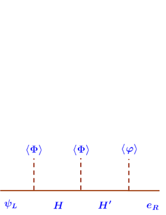
Figure 3: Diagram showing generation of the higher-dimensional operator ${\cal O}=\frac{\kappa(\mu)}{\Lambda^{2}}\,\bar{\psi}_{Li}\,\Phi_{ik}\,\Phi_{kj}\,\varphi\,e_{Rj}$ through see-saw mechanism. $H$ and $H^{\prime}$ denote heavy fermions to be integrated out.

On the other hand, the VEV $\langle\Phi\rangle$ is determined by minimizing the potential of scalar fields in each model. By deliberately choosing a specific form of the potential, the VEV is made to satisfy the relation

$$\frac{v_{1}(\mu)+v_{2}(\mu)+v_{3}(\mu)}{\sqrt{3\,[v_{1}(\mu)^{2}+v_{2}(\mu)^{2}+v_{3}(\mu)^{2}]}}=\frac{1}{\sqrt{2}}$$ (12)

in the basis where it is diagonal. Hence, the origin of Koide’s formula is attributed to the specific form of the potential which realizes this relation in the vacuum configuration. Up to now, however, no existing model is complete with respect to symmetry. Namely, every model requires either absence or strong suppression of some of the terms in the potential (which are allowed by the symmetry of that model), without justification.

In our study, we adopt a similar scenario for generating the charged lepton spectrum. We introduce a higher-dimensional operator similar to ${\cal O}$ of eq. (11) within an effective field theory (EFT) valid below some cut-off scale $\Lambda(\gg M_{W})$. We analyze a potential of scalar fields within this EFT and compute the spectrum of the charged leptons. We compute various radiative corrections and other types of corrections within this EFT.

In the next section (Sec. 2), we explain philosophy of our analysis using EFT and argue for its validity and usefulness. In Sec. 3, we explain the mechanism how to cancel the QED correction in terms of the radiative correction induced by family gauge symmetry. In Sec. 4, we present a potential model within EFT which leads to Koide’s mass formula and a realistic charged lepton spectrum. Summary and discussion are given in Sec. 5.

2 Why EFT? Virtue and assumptions

Let us explain philosophy of our analysis using EFT. Conventionally a more standard approach for explaining Koide’s mass formula has been to construct models within renormalizable theories. In comparison, it is certainly a retreat to make an analysis within EFT. Nevertheless, the long history since the discovery of Koide’s formula shows that it is quite difficult to construct a viable renormalizable model for explaining Koide’s relation. It is likely that we are missing some essential hints to achieve this goal, if the relation is not a sheer coincidence. The point we want to make through our study is that within EFT, explanation of Koide’s formula is possible, by largely avoiding fine tuning of parameters. Consistency conditions (with respect to symmetries of the theory) can be satisfied relatively easily in EFT, or in other words, they can be replaced by reasonable boundary conditions of EFT at the cut-off scale $\Lambda$ without conflicting symmetry requirements of the theory. (See Sec. 4.) Even under this less restrictive theoretical constraints, we may learn some important hints concerning the relation between the lepton spectrum and family symmetries. These are the role of specific family gauge symmetry in canceling the QED correction, the role of family symmetry in stabilizing Koide’s mass relation, or the role of family symmetry in realizing a realistic charged lepton spectrum consistently with experimental values. These properties do not come about separately but are closely tied with each other. These features do not seem to depend on details of more fundamental theory above the cut-off scale $\Lambda$ but rather on some general aspects of family symmetries and their breaking patterns. Thus, we consider that our approach based on EFT would be useful even in the case in which physics above the scale $\Lambda$ is obscure and may involve some totally unexpected ingredients —– as it was the case with chiral perturbation theory before the discovery of QCD.

Before discussing radiative corrections within EFT, one would be worried about effects of higher-dimensional operators suppressed in higher powers of $1/\Lambda$. Indeed, using the values of tau mass and the electroweak symmetry breaking scale $v_{\rm ew}$, one readily finds that $v_{3}/\Lambda\hbox{ \raise 3.0pt\hbox to0.0pt{$>$}\raise-3.0pt\hbox{$\sim$} }0.1$. Hence, naive dimensional analysis indicates that there would be corrections to Koide’s formula of order 10% even at tree level. We now argue that this is not necessarily the case within the scenario under consideration. Let us divide the corrections into two parts. These are (i) $1/\Lambda^{n}$ corrections to the operator $\cal O$ of eq. (11) (those operators which reduce to the SM Yukawa interactions after $\Phi$ is replaced by its VEV), and (ii) $1/\Lambda^{n}$ corrections to the relation (12) satisfied by the VEV of $\Phi$.

Concerning the corrections (i), we may consider the following example. Suppose that the operator $\cal O$ is induced from the interactions

$${\cal L}=y_{1}\,\bar{\psi}_{Li}\Phi_{ij}H_{Rj}+M\,\bar{H}_{Ri}H_{Li}+y_{2}\,\bar{H}_{Li}\Phi_{ij}H^{\prime}_{Rj}+M^{\prime}\bar{H}^{\prime}_{Ri}H^{\prime}_{Li}+y_{3}\,\bar{H}^{\prime}_{Li}\varphi e_{Ri}+({\rm h.c.})$$ (13)

through the diagram shown in Fig. 3, after fermions $H_{L,R}$ and $H^{\prime}_{L,R}$ have been integrated out. Fermions $H_{L,R}$ and $H^{\prime}_{L,R}$ are assigned to appropriate representations of the SM gauge group such that the above interactions become gauge singlet. For instance, in the case that $v_{3}/M^{\prime}\hbox{ \raise 3.0pt\hbox to0.0pt{$>$}\raise-3.0pt\hbox{$\sim$} }3$, $y_{1},y_{2},y_{3}\approx 1$ and $v_{\rm ew}/M^{\prime}<3\times 10^{-3}$, one finds, by computing the mass eigenvalues, that the largest correction to the lepton spectrum eq. (10) arises from the operator $\displaystyle-\frac{y_{1}^{3}y_{2}^{3}y_{3}}{2M^{3}M^{\prime 3}}\,\bar{\psi}_{L}\Phi^{6}\varphi e_{R}$; its contribution to the tau mass is $\delta m_{\tau}/m_{\tau}=(m_{\tau}/v_{\rm ew})^{2}\approx 5\times 10^{-5}$. This translates to a correction to Koide’s relation of $3\times 10^{-6}$, since there is an additional suppression factor due to the fact $m_{e},m_{\mu}\ll m_{\tau}$. Thus, this is an example of underlying mechanism that generates the operator $\cal O$ without generating higher-dimensional operators conflicting the current experimental bound. If we introduce even more (non–SM) fermions to generate the leading–order operator $\cal O$, one can always find a pattern of spectrum of these fermions, for which higher–dimensional operators are sufficiently suppressed, since the number of adjustable parameters increases. In general, sizes of higher-dimensional operators depend heavily on underlying dynamics above the cut-off scale. (See [11] for another example of underlying mechanism.)

Let us restrict ourselves within EFT. If we introduce only the operator $\cal O$, by definition this is the only contribution to the charged lepton spectrum at tree level. Whether loop diagrams induce higher-dimensional operators which violate Koide’s relation is an important question, and a detailed analysis is necessary. This is the subject of the present study, where the result depends on the mechanisms how Koide’s formula is satisfied and how the charged lepton spectrum is determined, even within EFT. The conclusion is as follows. Within the model to be discussed in Secs. 3–5, the class of 1-loop diagrams shown in Fig. 4 do not generate operators that violate Koide’s relation sizably; see Sec. 5. (There is another type of 1-loop diagrams that possibly cancels the QED correction; see Sec. 3.) We do not find any loop-induced higher-dimensional operators which violate Koide’s relation in conflict with the current experimental bound.

\psfrag{Phi}{$\Phi$}\psfrag{psiL}{$\psi_{L}$}\psfrag{eR}{$e_{R}$}\includegraphics[width=369.88582pt]{1LoopAnalyInEFT.eps}

Figure 4: EFT 1-loop diagrams which generate higher-dimensional operators contributing to the charged lepton spectrum. Dashed line represents $\Phi$; $\otimes$ represents the higher-dimensional operator which generate the charged lepton masses at tree-level [corresponding to ${\cal O}$ of eq. (11)].

Concerning the corrections (ii), we will introduce specific family gauge symmetries and their breaking patterns such that, in the first place the relation (12) is satisfied at tree level, and secondly the corrections (ii) are suppressed.

Since the above example of underlying mechanism that suppresses higher–dimensional operators is simple and fairly general, and since suppression of induced $1/\Lambda^{n}$ corrections within EFT provides a non–trivial cross check of theoretical consistency, we believe that our approach based on EFT has a certain justification and would be useful as a basis for considering more fundamental models.

3 Cancellation of QED corrections

In this section, we consider $U(3)$ family gauge symmetry and examine the radiative correction to Koide’s formula induced by the family gauge interaction. We denote the generators for the fundamental representation of $U(3)$ by $T^{\alpha}$ ($0\leq\alpha\leq 8$), which satisfy

$${\rm tr}\left(T^{\alpha}T^{\beta}\right)=\frac{1}{2}\,\delta^{\alpha\beta}~{}~{}~{};~{}~{}~{}T^{\alpha}={T^{\alpha}}^{\dagger}\,.$$ (14)

$T^{0}=\frac{1}{\sqrt{6}}{\bf 1}$ is the generator of $U(1)$, while $T^{a}$ ($1\leq a\leq 8$) are the generators of $SU(3)$. This fixes the normalization of the $U(1)$ charge.

We assign $\psi_{L}$ to the representation $({\bf 3},1)$, where $\bf 3$ stands for the $SU(3)$ representation and 1 for the $U(1)$ charge, while $e_{R}$ is assigned to $(\bar{\bf 3},-1)$. Under $U(3)$, the 9–component field $\Phi$ transforms as three $({\bf 3},1)$’s. $\varphi$ is singlet under $U(3)$. Explicitly the transformations of these fields are given by

$$\psi_{L}\to U\,\psi_{L}\,,~{}~{}~{}e_{R}\to U^{*}\,e_{R}\,,~{}~{}~{}\Phi\to U\,\Phi\,,~{}~{}~{}\varphi\to\varphi$$ (15)

with $U=\exp\left(i\theta^{\alpha}T^{\alpha}\right)$.

We consider

$${\cal O}_{1}=\frac{\kappa_{1}(\mu)}{\Lambda^{2}}\,\bar{\psi}_{L}\,\Phi\,\Phi^{T}\,\varphi\,e_{R}\,$$ (16)

as the higher-dimensional operator which generates the charged lepton spectrum at tree level [corresponding to $\cal O$ of eq. (11)]. It is invariant under the above $U(3)$ gauge symmetry, whereas $\cal O$ is not, since we assigned $\psi_{L}$ and $e_{R}$ to mutually conjugate representations. In fact, ${\cal O}_{1}$ is invariant under a larger symmetry $U(3)\times O(3)$, under which $\Phi$ transforms as $\Phi\to U\Phi O^{T}$ ($O\,O^{T}={\bf 1}$). In this section we ignore the $O(3)$ symmetry and focus on the $U(3)$ gauge symmetry. When $\Phi$ acquires a VEV

$$\langle\Phi(\mu)\rangle=\left(\begin{array}[]{ccc}v_{1}(\mu)&0&0\\ 0&v_{2}(\mu)&0\\ 0&0&v_{3}(\mu)\end{array}\right),$$ (20)

and if all $v_{i}$ are different, $U(3)$ symmetry is completely broken by $\langle\Phi\rangle$, and the spectrum of the $U(3)$ gauge bosons is determined by $v_{i}$.

With all this setup we may compute the radiative corrections to the pole masses induced by the family gauge interactions; see Fig. 5.

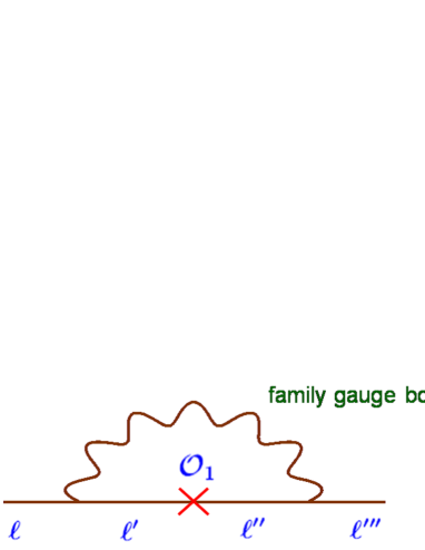
Figure 5: Diagram for the 1-loop correction to the charged lepton pole mass induced by exchange of family gauge bosons.

It turns out that the radiative corrections to the pole masses have the same form as the QED corrections eq. (6) with opposite sign:

$$\delta m^{\rm pole}_{i}=-\frac{3\,\alpha_{F}}{8\,\pi}\left[\log\left(\frac{\mu^{2}}{v_{i}(\mu)^{2}}\right)+c\right]\,{m}_{i}(\mu)\,,~{}~{}~{}~{}~{}~{}~{}{m}_{i}(\mu)=\frac{\kappa_{1}(\mu)\,v_{\rm ew}}{\sqrt{2}\Lambda^{2}}\,v_{i}(\mu)^{2}\,.$$ (21)

Here, $c$ is a constant independent of $i$. $\alpha_{F}=g_{F}^{2}/(4\pi)$ denotes the coupling constant of the $U(3)$ gauge symmetry, where we assume that the couplings of $U(1)$ and $SU(3)$ are common. The Wilson coefficient $\kappa_{1}(\mu)$ is defined in $\overline{\rm MS}$ scheme. $v_{i}(\mu)$ are defined as follows: The VEV of $\Phi$ at renormlization scale $\mu$, $\langle\Phi(\mu)\rangle$ given by eq. (20), is determined by minimizing the 1–loop effective potential in Landau gauge (explicit form of the effective potential will be discussed in the next section); $\Phi$ is renormalized in $\overline{\rm MS}$ scheme. We ignored terms suppressed by ${m}_{i}^{2}/v_{j}^{2}(\ll 1)$ in the above expression.

Some important features are as follows.

1. The sign is opposite to that of the QED correction eq. (6), which results from the fact that $\psi_{L}$ and $e_{R}$ have the same QED charges but mutually conjugate (opposite) $U(3)$ charges.

2. Suppose the relation (12) is satisfied at tree level, such that Koide’s formula is satisfied. Then there is no ${\cal O}(\alpha_{F})$ correction to this relation. (Recall that the correction to the 1-loop effective potential in Landau gauge à la Coleman-Weinberg is ${\cal O}(\alpha_{F}^{2})$.)

3. The characteristic form of the radiative corrections eq. (21) is determined by the fact that ${\cal O}_{1}$ is multicatively renormalized, and also by the symmetry breaking pattern $U(3)\to U(2)\to U(1)\to\mbox{nothing}$.

4. In the case that $\alpha=\frac{1}{4}\alpha_{F}$, the radiative corrections by family gauge interactions and the QED corrections to Koide’s mass formula cancel for arbitrary $\mu$.

Let us add some explanation on the feature 3.

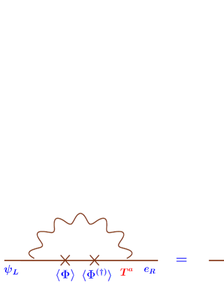
(a)

(b)

Figure 6: 1–loop diagrams contributing to $\delta m_{i}^{\rm pole}$, (a) in the case that $\psi_{L}$ and $e_{R}$ are in the same representation of $SU(3)$ or $O(3)$, i.e. $\psi_{L}:({\bf 3},Q)$ and $e_{R}:({\bf 3},Q^{\prime})$, and (b) in the case that $\psi_{L}$ and $e_{R}$ are in the conjugate representations of $U(3)$, i.e. $\psi_{L}:({\bf 3},1)$ and $e_{R}:(\bar{\bf 3},-1)$. The right–hand–sides show flows of family charge. In (a), the closed loop of the family charge flow represents ${\rm tr}\bigl{(}\Phi\Phi^{(\dagger)}\bigr{)}$. In (b), the charge flow is connected in one line, which has the same form as the tree diagram, showing multiplicative renormalization of the operator ${\cal O}_{1}$.

The operator ${\cal O}_{1}$ is the only dimension-6 operator invariant under $U(3)\times O(3)$, so it should be renormalized multiplicatively. In this regard, a pedagogical comparison is shown in Figs. 6(a)(b). Had we chosen the same representation for $\psi_{L}$ and $e_{R}$ under family symmetry such as $SU(3)$ or $O(3)$, the dimension-4 operator $\bar{\psi}_{Li}\varphi e_{Ri}$ would be allowed by symmetry [15]. In fact, the 1–loop diagram shown in Fig. 6(a) induces an effective operator

$${\cal O}^{\prime}\sim\frac{\alpha_{F}}{\pi}\times{\kappa}\,\bar{\psi}_{Li}\,\varphi\,e_{Ri}\times\frac{\langle\Phi\rangle_{jk}\langle\Phi^{(\dagger)}\rangle_{kj}}{\Lambda^{2}}\,,$$ (22)

hence corrections universal to all the charged–lepton masses, $(\delta m_{e},\delta m_{\mu},\delta m_{\tau})\propto(1,1,1)$, are induced. This correction changes the direction of $(\sqrt{m_{e}},\sqrt{m_{\mu}},\sqrt{m_{\tau}})$ and violates Koide’s formula rather strongly; moreover the correction is dependent on the cut-off $\Lambda$ of the loop integral. In order that the correction to Koide’s formula cancel the QED correction, a naive estimate shows that $\alpha_{F}/\pi$ should be order $10^{-5}$, provided that $\Lambda$ is not too large. By contrast, in the case that $\psi_{L}$ and $e_{R}$ are assigned to the conjugate representations of $U(3)$, the charge flow is connected in one line, so that it has the same charge flow structure as the tree graph. The form $\sim\log\mu\times m_{i}$ of the 1-loop correction can be understood in this way.

$v_{i}^{2}$ in the argument of log in eq. (21) stems from IR cut-off of the loop integral. Namely they come from the masses of family gauge bosons. As $v_{3}>v_{2}>v_{1}>0$ are successively turned on, family symmetry breaks according to the pattern $U(3)\to U(2)\to U(1)\to\mbox{nothing}$. Gauge bosons corresponding to broken generators decouple at each stage, and their masses enter the argument of log as IR cut-off. The form of eq. (21) is essentially determined by this symmetry breaking pattern. (See [2] for a more precise argument.) The same symmetry breaking pattern resides in the QED Lagrangian: as $m_{\tau}>m_{\mu}>m_{e}>0$ are successively turned on, chiral symmetry breaks according to $U(3)\to U(2)\to U(1)\to\mbox{nothing}$. Essentially this is the reason why the two radiative corrections have the same form.

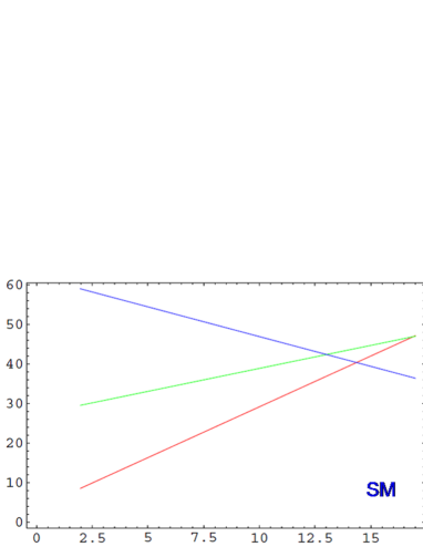
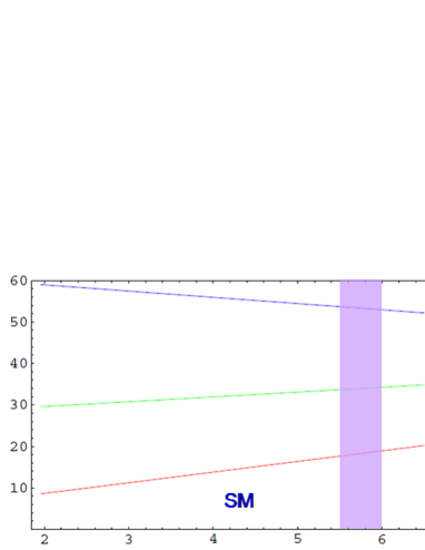
(a)		(b)

Figure 7: Inverse of the three gauge couplings of the SM $\alpha_{1}^{-1},\alpha_{2}^{-1},\alpha_{3}^{-1}$ vs. $\log_{10}(\mu/{\rm GeV})$: (a) from electroweak scale to GUT scale, and (b) from electroweak scale up to $10^{3}$ TeV. The green line corresponds to the relevant coupling $\alpha_{W}$. The shaded band shows an allowed variation range of the unification scale in order to meet the present experimental accuracy of Koide’s formula.

Now we speculate on a possible scenario how the relation (feature 4)

$$\alpha\approx\frac{1}{4}\alpha_{F}$$ (23)

may be satisfied. In fact, this relation should be satisfied within 1% accuracy, in order that Koide’s relation is satisfied within the present experimental bound. As already discussed, the scale of $\alpha$ is determined by the charged lepton masses, while the scale of $\alpha_{F}$ is determined by the family gauge boson masses, which should be much higher than the electroweak scale. Since the relevant scales of the two couplings are very different, we are unable to avoid assuming some accidental factor (or parameter tuning) to achieve this condition. Instead we seek for an indirect evidence which indicates such an accident has occurred in Nature. The relation (23) shows that the value of $\alpha_{F}$ is close to that of the weak gauge coupling constant $\alpha_{W}$, since $\sin^{2}\theta_{W}(M_{W})$ is close to $1/4$. In fact, within the SM, $\frac{1}{4}\,\alpha_{W}(\mu)$ approximates $\alpha(m_{\tau})$ at scale $\mu\sim 10^{2}$–$10^{3}$ TeV. Hence, if the electroweak $SU(2)_{L}$ gauge group and the $U(3)$ family gauge group are unified around this scale, naively we expect that $\alpha\approx\frac{1}{4}\,\alpha_{F}$ is satisfied. Since $\alpha_{W}$ runs relatively slowly in the SM, even if the unification scale is varied within a factor of 3, Koide’s mass formula is satisfied within the present experimental accuracy. This shows the level of parameter tuning required in this scenario. Fig. 7(a)(b) show the running of the inverse of the three gauge couplings of the SM. The former figure is well-known, which shows the running from the electroweak scale up to GUT scale. The latter figure shows the same running up to $10^{3}$ TeV. The shaded band shows an allowed variation range (factor 3) of the unification scale, which is limited by the present experimental accuracy of Koide’s formula.

4 Potential predicting Koide’s formula and realistic lepton spectrum

In this section we study how the relation (12) can be satisfied by the VEV of $\Phi$. For this purpose, we introduce a model of charged lepton sector based on $U(3)\times O(3)$ family gauge symmetry, within EFT valid at scales below $\Lambda$. The choice of this family symmetry is motivated by the fact that this is the largest symmetry possessed by the operator ${\cal O}_{1}$ analyzed in the previous section. In particular, in this section we focus on the potential of scalar fields. In the first place, we find that the $U(3)\times O(3)$ family symmetry is not sufficiently restrictive. Namely, since this symmetry does not constrain the potential of $\Phi$ sufficiently, one needs to tune the parameters of the potential in order to realize the relation (12). We need some symmetry enhancement in order to realize this relation without fine tuning.

\psfrag{45}{$45^{\circ}$}\psfrag{Phi0}{$\Phi^{0}T^{0}$}\psfrag{Phia}{$\Phi^{a}T^{a}$}\psfrag{Phimu}{$\Phi^{\alpha}T^{\alpha}$}\includegraphics[width=170.71652pt]{PhiIn9dimSp.eps}

Figure 8: Geometrical interpretation of eq. (25). Eq. (14) defines the inner product in a 9–dimensional real vector space spanned by the basis $\{T^{\alpha}\}$. Since $\Phi^{0}T^{0}$, $\Phi^{a}T^{a}$ and $\Phi=\Phi^{\alpha}T^{\alpha}$ form an isosceles right triangle, the angle between $T^{0}$ and $\Phi$ is $45^{\circ}$. This is Koide’s formula in the basis where $\Phi$ is diagonal.

In order to find an appropriate larger symmetry, we recall the conditions equivalent to the relation (12). Let us express components of $\Phi$ using $T^{\alpha}$, introduced in eq. (14), as the basis:

$$\Phi=\Phi^{\alpha}\,T^{\alpha}\,.$$ (24)

In general $\Phi^{\alpha}$ take complex values. As shown by Koide [13], if

$$(\Phi^{0})^{2}=\Phi^{a}\,\Phi^{a}~{}~{}~{}~{}~{};~{}~{}~{}~{}~{}\Phi^{\alpha}\in{\bf R}\,$$ (25)

are satisfied, the relation (12) is satisfied by the eigenvalues of $\Phi$. There is a geometrical interpretation of these conditions in terms of a real vector in a 9-dimensional space; see Fig. 8. This picture indicates that a symmetry associated with this 9-dimensional space may be relevant.

Motivated by this picture, we adopt $SU(9)\times U(1)$ as an enhanced symmetry, where the $SU(9)\times U(1)$ transformation is given by $\Phi^{\alpha}\to U_{9}^{\alpha\beta}\,\Phi^{\beta}$ ($U_{9}$ is a 9-by-9 unitary matrix). Then we assume the following symmetry breaking scenario: Above the cut–off scale $\Lambda$ there is an $SU(9)\times U(1)$ gauge symmetry, and this symmetry is spontaneously broken to $U(3)\times O(3)$ below the cut–off scale; see Fig. 9. One can check that indeed $U(3)\times O(3)$ is a subgroup of $SU(9)\times U(1)$.

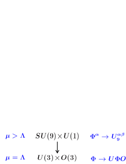
Figure 9: Symmetry breaking pattern assumed in our senario.

In what follows, we do not discuss any specific model at scales above $\Lambda$ but only assume restoration of this larger symmetry.

Within this senario, we still need to introduce an additional scalar field $X$ in order to realize a desirable vacuum configuration. Under $SU(9)\times U(1)$, $X$ is in the representation $({\bf 45},Q_{X})$ (the ${\bf 45}$ is the second–rank symmetric representation) and is unitary. It can be represented by a 9–by–9 unitary symmetric matrix:

$$X^{\alpha\beta}=X^{\beta\alpha},~{}~{}~{}~{}~{}X^{\alpha\gamma}\,{X^{\beta\gamma}}^{*}=\delta^{\alpha\beta}~{}~{}~{}~{}~{};~{}~{}~{}~{}~{}X^{\alpha\beta}\to{U}_{9}^{\alpha\rho}\,X^{\rho\sigma}\,{U}_{9}^{\beta\sigma}\,.$$ (26)

Note that the unitarity condition is compatible with the symmetry transformation.

We have analyzed the potential of $\Phi$ and $X$ that is invariant under $U(3)\times O(3)$ and consistent with the assumed symmetry breaking pattern shown schematically in Fig. 9. The upshot is that in a finite region of the parameter space of the potential Koide’s relation is satisfied by the eigenvalues of $\langle\Phi\rangle$. Furthermore, the eigenvalues can be made consistent with the experimental values of the charged lepton masses without fine tuning of parameters. In the rest of this section we briefly sketch the argument. (See [2] for details.)

Operators in the potential which are invariant under $SU(9)\times U(1)$ read

$$\tilde{V}_{\Phi}=-m^{2}\,{\Phi^{\alpha}}^{*}\Phi^{\alpha}+\lambda\,({\Phi^{\alpha}}^{*}\Phi^{\alpha})^{2}+\cdots\,,$$ (27)

$$\tilde{V}_{X}={\rm const.}\,,$$ (28)

$$\tilde{V}_{\Phi X}=\varepsilon_{K}\,\bigl{|}\Phi^{\beta}\,{X^{\beta\gamma}}^{*}\,\Phi^{\gamma}\bigr{|}^{2}+\cdots\,,$$ (29)

where only some representative terms have been shown explicitly. In particular, we take into account operators with dimensions higher than 4, although they are not shown explicitly. That $\tilde{V}_{X}={\rm const.}$ follows from the fact that $X$ is unitary and has a non-vanishing $U(1)$ charge. Similarly operators invariant under $U(3)\times O(3)$ but non-invariant under $SU(9)\times U(1)$ read

$$V_{\Phi}=g_{1}\,{\rm tr}(\Phi^{\dagger}\,\Phi\,\Phi^{\dagger}\,\Phi)+g_{2}\,{\rm tr}(\Phi\,\Phi^{T}\,\Phi^{*}\,\Phi^{\dagger})+\cdots\,,$$ (30)

$$V_{X}=h_{1}\,{\rm tr}(T^{\alpha}\,T^{\rho}\,T^{\beta}\,T^{\sigma})\,X^{\alpha\beta}\,{X^{\rho\sigma}}^{*}\,+\cdots\,,$$ (31)

$$V_{\Phi X}=\cdots\,.$$ (32)

After examination, we find that, in a certain parameter region, the global minimum of $V_{X}$ is located at the configuration

$$\langle X^{\alpha\beta}\rangle={\rm diag.}(-1,\underbrace{+1,\cdots,+1}_{{8}})=-2\,\delta^{\alpha 0}\delta^{\beta 0}+\delta^{\alpha\beta}\,,$$ (33)

and $\tilde{V}_{\Phi X}$ is minimized in the case

$$\Phi^{\beta}\,{X^{\beta\gamma}}^{*}\,\Phi^{\gamma}=0\,,$$ (34)

as may be inferred from the term of $\tilde{V}_{\Phi X}$ shown explicitly. One observes that if the above two equations are combined, Koide’s relation

$$(\Phi^{0})^{2}=\Phi^{a}\,\Phi^{a}$$ (35)

follows. (Reality of $\Phi$ can also be derived from $\tilde{V}_{\Phi}$ and $V_{\Phi X}$, but we skip explanation of this part.)

Let us first give an argument which is not very solid but more illustrative. The above observation shows that if there is a hierarchy of parameters given by

$$\tilde{m}^{2},\lambda,\varepsilon_{K},\tilde{h}_{1}\gg g_{1},g_{2}\,,$$ (36)

while ignoring all the other parameters, Koide’s mass formula will be satisfied approximately. Here, $\tilde{m}^{2}$ and $\tilde{h}_{1}$ denote dimensionless couplings defined from $m^{2}$ and $h_{1}$, respectively, after rescaling them by an appropriate mass scale (e.g. $v_{3}$). Furthermore, we find that if there is an additional hierarchy given by

$$\tilde{m}^{2},\lambda,\varepsilon_{K},\tilde{h}_{1}\gg g_{2}\gg g_{1}\,,$$ (37)

a realistic charged lepton spectrum $v_{1}:v_{2}:v_{3}=\sqrt{m_{e}}:\sqrt{m_{\mu}}:\sqrt{m_{\tau}}$ can be explained without fine tuning. (This follows from an explicit computation, and we do not know any other simple explanation.) Naively one may expect that the parameters in the $SU(9)\times U(1)$ non-invariant operators $g_{1},g_{2},\tilde{h}_{1}$ are suppressed as compared to the parameters in the $SU(9)\times U(1)$ invariant operators $\tilde{m}^{2},\lambda,\varepsilon_{K}$, since the former parameters are generated only through spontaneous symmetry breaking at the cut-off scale. But this is not necessarily the case for parameters such as $\tilde{h}_{1}$ that are originally dimensionful parameters. Let us speculate on a possible underlying mechanism that would lead to a hierarchy of potential parameters given by eq. (37).

Suppose that the symmetry breaking $SU(9)\times U(1)\to U(3)\times O(3)$ is induced by a condensate of a scalar field $T^{\alpha\beta}_{\rho\sigma}$, which is a 4th-rank tensor under $SU(9)$. Indeed if $\langle T^{\alpha\beta}_{\rho\sigma}\rangle\sim{\rm tr}(T^{\alpha}{T^{\beta}}^{*}{T^{\rho}}^{*}T^{\sigma})$, this symmetry breaking takes place.

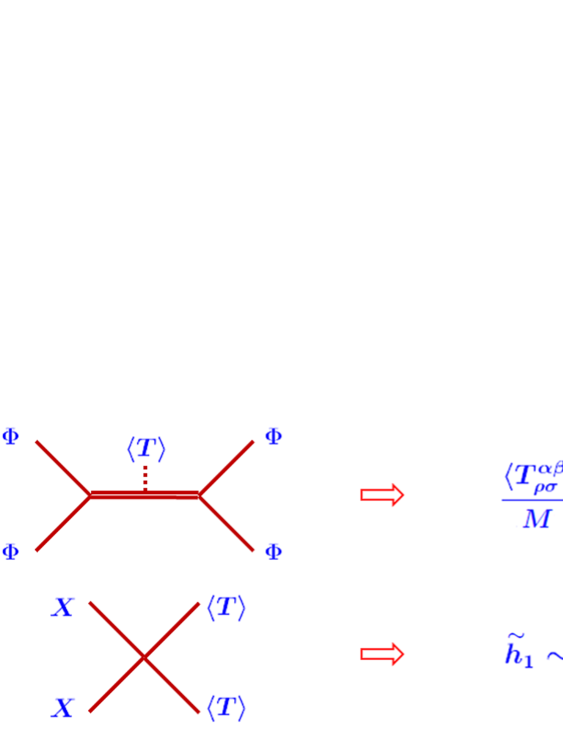
Figure 10: Speculation on underlying physics that may generate $SU(9)\times U(1)$ non-invariant operators.

Through the first diagram shown in Fig. 10, the operator $g_{2}\,{\rm tr}(\Phi\,\Phi^{T}\,\Phi^{*}\,\Phi^{\dagger})$ may be induced; the double line denotes a heavy degree of freedom with an $SU(9)\times U(1)$-invariant mass scale $M$. Since $\langle T\rangle\sim{\cal O}(\Lambda)$, the coefficient $g_{2}\sim\Lambda/M$ would be a small parameter provided $M\gg\Lambda$. $g_{1}$ is even more suppressed, since the operator $g_{1}\,{\rm tr}(\Phi^{\dagger}\,\Phi\,\Phi^{\dagger}\,\Phi)$ cannot be generated by a single insertion of $\langle T\rangle$ at tree-level. Either two insertions of $\langle T\rangle$ or a loop correction is necessary, which leads to additional suppression factors. The second diagram in Fig. 10 would induce the operator $h_{1}\,{\rm tr}(T^{\alpha}\,T^{\rho}\,T^{\beta}\,T^{\sigma})\,X^{\alpha\beta}\,{X^{\rho\sigma}}^{*}$ (together with other operators). Since there is no intermediate heavy degree of freedom, the induced coupling $h_{1}$, when normalized by $\Lambda$, would be order 1.

We turn to a more solid argument. It is legitimate to identify the above potential to be the effective potential (including loop corrections and in Landau gauge). Recall that, according to the argument in Sec. 3, we can connect the pole masses of the charged leptons to the VEV of $\Phi$, which is determined from the effective potential renormalized at an arbitrary scale $\mu$. For our purpose, it is most convenient to set the scale to be $\mu=\Lambda$, since at this scale radiative corrections within EFT essentially vanish, and the parameters of the effective potential are set by the boundary (initial) conditions derived from the theory above the cut-off scale.

The following conclusions have been drawn from a detailed analysis of the general potential of $\Phi$ and $X$. In the case that certain hierarchical relations among the parameters of the potential are satisfied, Koide’s formula as well as a realistic charged lepton spectrum follow, consistently with the present experimental values. These hierarchical conditions on the parameters are a generalization of eq. (37). Typical sizes of the required hierarchies of the potential parameters are of order $10^{-3}$–$10^{-4}$. These hierarchical relations are consistent with the assumed symmetry and symmetry enhancement. Namely, those parameters which need to be suppressed are associated with $SU(9)\times U(1)$ non-invariant operators. Their values at the boundary $\mu=\Lambda$ are determined by the dynamics above the cut-off scale. On the other hand, up to now there exists no model of the scales above the cut-off, $\mu>\Lambda$, which leads to these hierarchical relations among the potential parameters. (Nothing more than the speculation given in Fig. 10 exists.)

Finally we comment on how a realistic charged lepton spectrum follows without fine tuning of parameters. Koide’s formula imposes one relation among the three charged lepton masses. Hence, apart from an overall dimensionful scale of the three masses, there remains one-parameter degree of freedom. Suppose this degree of freedom is fixed by minimizing the operator $V_{\Phi 3}=g_{2}\,{\rm tr}(\Phi\,\Phi^{T}\,\Phi^{*}\,\Phi^{\dagger})$. Then, $m_{e}/m_{\tau}$ is predicted to be 15% away from the experimental value, and $m_{\mu}/m_{\tau}$ is predicted to be 1.5% away from the experimental value. In other words, already the values are close to the true values and orders of magnitude of the mass ratios are predicted correctly. When any other $SU(9)\times U(1)$ non-invariant operators, which modify the potential minimum, are turned on, as long as contributions of these operators are suppressed as compared to $V_{\Phi 3}$, the values of $m_{e}/m_{\tau},m_{\mu}/m_{\tau}$ do not alter significantly. Since Koide’s relation is protected by the large couplings (e.g. $\tilde{m}^{2},\lambda,\varepsilon_{K},\tilde{h}_{1}$), and since Koide’s relation is satisfied experimentally, with some small values of parameters, $m_{e}/m_{\tau}$ and $m_{\mu}/m_{\tau}$ are designated to coincide with the experimental values. This is not regarded as fine tuning. The overall scale of the lepton masses is determined by the parameters of $\tilde{V}_{\Phi}$, such as $m^{2}$ and $\lambda$, and by $\kappa_{1}$ of the operator ${\cal O}_{1}$. Since $v_{3}/\Lambda\hbox{ \raise 3.0pt\hbox to0.0pt{$>$}\raise-3.0pt\hbox{$\sim$} }0.1$ is not extremely small, there is no fine tuning problem within EFT for predicting the overall scale.

5 Summary and discussion

Let us summarize our study. We have analyzed the role of family gauge symmetries in relation with the charged lepton spectrum and Koide’s mass formula. The analysis is performed within EFT valid below a cut-off scale $\Lambda$ and within the known scenario in which the charged lepton mass matrix is proportional to $\langle\Phi\rangle^{2}$ at leading order. Before describing the analysis, we made an argument to justify usefulness of an EFT approach and to discuss why EFT does not instantly run into problems by higher order corrections in $1/\Lambda$.

In the first part of our analysis, we studied radiative corrections generated by $U(3)$ family gauge interaction. $U(3)$ family gauge symmetry has a unique property with respect to the radiative correction to Koide’s formula. In fact, if $\psi_{L}$ and $e_{R}$ are assigned to mutually conjugate representations, the $U(3)$ radiative correction has the same form as the QED correction with opposite sign. In particular, if $\alpha=\frac{1}{4}\alpha_{F}$, both corrections cancel. We discussed this possibility within a scenario in which $U(3)$ family symmetry is unified with $SU(2)_{L}$ symmetry at $10^{2}$–$10^{3}$ TeV scale.

Some key aspects which led to the non-trivial form of the radiative corrections are as follows. (1) Multiplicative renormalizability of the operator ${\cal O}_{1}=\frac{\kappa}{\Lambda^{2}}\,\bar{\psi}_{L}\,\Phi\,\Phi^{T}\,\varphi\,e_{R}$ ensures that only logarithmic corrections to the lepton mass matrix appear; furthermore, multiplicative renormalizability of $\langle\Phi\rangle$ ensures that the correction to Koide’s formula is independent of the renormalization scale $\mu$ of the effective potential. (2) The symmetry breaking pattern $U(3)\to U(2)\to U(1)\to\mbox{(nothing)}\,$ essentially dictates how the IR cut-off enters the logarithmic correction at each stage of the symmetry breaking; this symmetry breaking pattern happens to be common to the family gauge sector and QED sector. (3) We assumed that $\langle\Phi\rangle$ can be brought to a diagonal form by symmetry transformation and also the tree-level Koide’s relation for the diagonal elements: $\frac{v_{1}(\mu)+v_{2}(\mu)+v_{3}(\mu)}{\sqrt{3\,[v_{1}(\mu)^{2}+v_{2}(\mu)^{2}+v_{3}(\mu)^{2}]}}=\frac{1}{\sqrt{2}}$.

In the latter part of the analysis, we have examined how this relation among $v_{i}$ may be realized. We proposed a potential model within EFT with a family symmetry $U(3)\times O(3)$. Motivated by a geometrical interpretation of Koide’s relation (c.f. Fig. 8), we further imposed symmetry enhancement to $SU(9)\times U(1)$ above the cut-off scale. We have introduced another scalar field $X$ and examined the general potential of $\Phi$ and $X$. In this manner, we were able to find a potential minimum which leads to Koide’s formula and a realistic charged lepton spectrum. The potential parameters need to satisfy certain hierarchical relations at the boundary $\mu=\Lambda$ of EFT, which are consistent with the symmetry requirements. We have speculated on underlying physics which may lead to the hierarchical relations.

There are many unsolved questions in the present analysis. The list is as follows.

• Quarks and neutrinos are not included in the analysis. In relation to this, with the fermion content discussed in this analysis, anomalies induced by the family gauge interactions do not cancel.

• $O(3)$ gauge symmetry needs to be broken spontaneously above the $U(3)$ symmetry breaking scale, in order to suppress mixing of gauge bosons of both gauge groups. We have not implemented a mechanism to achieve this.

• The VEV $\langle\Phi\rangle$, which explains the realistic charged lepton spectrum, cannot be diagonalized by $U(3)\times O(3)$ symmetry transformation. In order to realize the scenario for the cancellation of QED correction, we need, for instance, to introduce another field $\Sigma$ and its potential with $\Phi$ [2] and replace the operator ${\cal O}_{1}$ as $\frac{\kappa}{\Lambda^{2}}\,\bar{\psi}_{L}\,\Phi\,\Phi^{T}\,\varphi\,e_{R}\to\frac{\kappa}{\Lambda^{3}}\,\bar{\psi}_{L}\,\Phi\,\Sigma\,\Phi^{T}\,\varphi\,e_{R}$.

• In the first part of our analysis, we considered unification of $U(3)$ family symmetry and $SU(2)_{L}$ weak symmetry. In the latter part, we assumed embedding $U(3)\times O(3)$ into $SU(9)\times U(1)$. How to make both scenario compatible has not been addressed. It would require a large symmetry group above the cut-off scale.

• Fine tuning is required to stabilize small scales compared to the cut-off scale of EFT $\Lambda\sim 10^{3}$ TeV. These small scales are the VEVs $\langle\varphi\rangle$, (physical scale of) $\langle X\rangle$ and $\langle\Sigma\rangle$. This fine tuning problem is similar to that of the SM.

• Models above the cut-off scale are completely missing.

There seems to be certain solution(s) to each of these problems (except for the last two problems), if we extend our model in a sufficiently complicated manner. On the other hand, it seems very difficult to solve all of them in a simple and unified way.

We have made a non-trivial consistency check of our present analysis. Using the potential of $\Phi$ and $X$, we have identified the mass eigenstates of scalar fields at the vacuum; then we have computed 1-loop radiative correction to the operator ${\cal O}^{\prime}_{1}=\frac{\kappa}{\Lambda^{3}}\,\bar{\psi}_{L}\,\Phi\,\Sigma\,\Phi^{T}\,\varphi\,e_{R}$ by these scalars. This corresponds to incorporating the class of diagrams shown in Fig. 4. The correction to Koide’s formula turned out to be quite suppressed and does not conflict the present experimental bound.

In view of the many problems listed above, it seems quite unlikely that our model, as a whole, correctly describes the true mechanisms of generation of the charged lepton spectrum. Nevertheless, we suspect that some of the mechanisms which we proposed may reflect the true aspects of Nature. We consider the following feature particularly non-trivial: Not only Koide’s formula but also $m_{e}/m_{\tau}$ and $m_{\mu}/m_{\tau}$ can be explained without fine tuning. Since Koide’s relation treats $m_{e},m_{\mu},m_{\tau}$ symmetrically, in many models hierarchical structure of the spectrum is difficult to realize compatibly with Koide’s relation, without fine tuning of parameters. As a final remark, we note that some phenomenological implications of the present scenario have been discussed in [2].

References

- [1] Y. Sumino, Phys. Lett. B 671, 477 (2009).
- [2] Y. Sumino, arXiv:0812.2103 [hep-ph].
- [3] Y. Koide, Nuovo Cim. A 70 (1982) 411 [Erratum-ibid. A 73 (1983) 327].
- [4] R. Foot, arXiv:hep-ph/9402242.
- [5] C. Amsler et al. [Particle Data Group], Phys. Lett. B 667 (2008) 1.
- [6] Y. Koide, Phys. Rev. D 28 (1983) 252; S. Esposito and P. Santorelli, Mod. Phys. Lett. A 10 (1995) 3077.
- [7] Y. Koide and M. Tanimoto, Z. Phys. C 72, 333 (1996).
- [8] For a review, see Y. Koide, arXiv:hep-ph/0506247.
- [9] N. Li and B. Q. Ma, Phys. Rev. D 73 (2006) 013009.
- [10] Z. z. Xing and H. Zhang, Phys. Lett. B 635 (2006) 107.
- [11] E. Ma, Phys. Lett. B 649 (2007) 287.
- [12] For recent works, see G. Rosen, Mod. Phys. Lett. A 22 (2007) 283; Y. Koide, Phys. Lett. B 665 (2008) 227; J. Phys. G 35 (2008) 125004; Phys. Rev. D 78 (2008) 093006; arXiv:0811.3470 [hep-ph]; N. Haba and Y. Koide, Phys. Lett. B 659 (2008) 260; JHEP 0806 (2008) 023, and references therein.
- [13] Y. Koide, Mod. Phys. Lett. A 5 (1990) 2319.
-
[14]
Y. Koide and H. Fusaoka,
Z. Phys. C 71 (1996) 459;
Y. Koide and M. Tanimoto,
Z. Phys. C 72 (1996) 333.
See also [8] and references therein. - [15] There are a large number of papers on the fermion flavor structure based on or family symmetry. See, for instance, Z. G. Berezhiani and M. Y. Khlopov, Sov. J. Nucl. Phys. 51 (1990) 739; S. F. King, JHEP 0508 (2005) 105; I. de Medeiros Varzielas and G. G. Ross, Nucl. Phys. B 733 (2006) 31; T. Appelquist, Y. Bai and M. Piai, Phys. Rev. D 74 (2006) 076001; S. Antusch, S. F. King and M. Malinsky, JHEP 0806 (2008) 068, and references therein.