GR models of the X-ray spectral variability of MCG–6-30-15

Abstract

Context. The extremely relativistic Fe lines, detected from some active galactic nuclei (AGN), indicate that generation and reprocessing of the X-ray emission takes place in the immediate vicinity of the event horizon. Recently, general relativistic (GR) effects, in particular light bending which is very strong in that region, have been considered to be the cause of complex variability patterns observed in these AGNs.

Aims. We study in detail the GR models of the X-ray spectral variability for various geometries of the X-ray source and with various relativistic effects being the dominant cause of spectral variability. The predicted properties are compared with the observational data of the Seyfert 1 galaxy MCG–6-30-15, which is currently the best studied AGN with signatures of strong gravity effects.

Methods. We focus on modeling the root mean square (RMS) spectra. We compute the RMS spectra for the GR models using a Monte Carlo method, and compare them with the RMS spectra from the Suzaku observations of MCG–6-30-15 on January 2006.

Results. The data disfavor models with the X-ray source (1) moving vertically on the symmetry axis or (2) corotating with the disc and changing height not far above the disc surface. The most likely explanation for the observed fractional variability is given by the model involving the X-ray source located at a very small, varying distance from a rapidly rotating black hole. This model predicts some enhanced variations in the red wing of the Fe line, which are not seen in the Suzaku observations. However, the enhanced variability of the red wing, while ruled out by the Suzaku data, is consistent with an excess RMS variability, between 5 and 6 keV, reported for some previous ASCA and XMM observations. We speculate that the presence or lack of such a feature is related to the change of the ionization state of the innermost part of the disc, however, investigation of such effects is currently not possible in our model (where a neutral disc is assumed). If the model, completed by a description of ionization effects, proves to be fully consistent with the observational data, it will provide a strong indication that the central black hole in MCG–6-30-15 rotates rapidly, supporting similar conclusions derived from the Fe line profile.

1 Introduction

AGNs are powerful sources of strongly variable X-ray emission, most likely originating close to a central black hole. The origin of the X-ray variability is poorly understood, however, some of the observed variations are supposed to be directly related to strong gravity effects and their investigation may give insight into properties of the space-time metric in the vicinity of the event horizon.

The bright Seyfert 1 galaxy MCG–6-30-15 ($z=0.00775$) is the key object for such studies. Its X-ray spectrum shows an extremely distorted Fe K$\alpha$ line, indicating that X-ray reprocessing takes place very close to the central black hole (e.g. Fabian et al. 2002; Miniutti et al. 2007). Furthermore, crucially for investigation of strong gravity in MCG–6-30-15, radiation reflected from the inner disc is not contaminated by radiation reflected from distant matter (see Sect. 4.2). The disc-line model for the detected line profile requires that roughly half of the observed Fe photons come from the innermost parts of the accretion disc, within 6 gravitational radii (these photons form the red wing of the line, below 6 keV) and the remaining from a slightly more distant region, at a few tens of gravitational radii (forming the blue peak, observed between 6 and 7 keV).

The time-resolved X-ray spectra in MCG–6-30-15 indicate that the best explanation of its spectral variability pattern is given by a phenomenological, two-component model consisting of (i) a highly variable power-law continuum (referred to as primary emission) and (ii) a much less variable, and uncorrelated, component with a spectrum characteristic of radiation reflected from the inner disc (e.g. Fabian & Vaughan 2003, Vaughan & Fabian 2004, Larsson et al. 2007; an alternative explanation, proposed by Miller et al. 2008, is briefly discussed in Sect. 5.6). The latter component includes both the Fe K$\alpha$ line and the associated Compton reflection hump, peaking around 30 keV, produced by down-scattering of higher energy photons. The varying relative contributions of these spectral components can explain the observed hardening of the X-ray spectrum at lower fluxes as well as reduced variations of the blue peak of the Fe K$\alpha$ line.

The apparent lack of connection between the two components indicates that some complex physical mechanism should be involved, as the components are supposed to originate together in the central region and a strict correlation between them would be expected in a simple reflection picture. Fabian & Vaughan (2003) first argued that this disconnectedness may be explained by relativistic effects, in particular by light bending and focusing of the primary emission towards the accretion disc. In this scenario, elaborated under some specific assumptions by Miniutti & Fabian (2004, MF04), the change of the height of the primary X-ray source is the cause of spectral variations.

However, a systematic investigation of this class of models by Niedźwiecki & Życki (2008, NZ08) questioned their ability to explain the observed effects. In particular, MF04 assess the reduced variability of the reflected component based on the behavior of the total flux of fluorescent photons received by a distant observer. NZ08 point out that changes of the height of the source induce substantial changes in the line profile, with significant variations of the fluxes in the blue peak and in the red wing. These balance each other for some range of parameters, reducing variations of the total flux, however, this property is not sufficient to explain the observed data. Then, the model fails to reproduce the key property which motivated its development, i.e. reduced variation of the blue peak of the Fe line.

Interestingly, NZ08 find an alternate model, which can explain reduced variations of the blue peak. The model proposed in NZ08 follows the generic idea of Fabian & Vaughan (2003), involving a scenario where the change of position of the primary source leads to large changes of directly observed emission and smaller changes of the amount received by the disc. However, the model assumes changes of the radial distance rather than the height and its properties rely on a qualitatively distinct effect, namely bending to the equatorial plane of the Kerr space-time. The model proposed in NZ08 predicts, however, some enhanced variations of the red wing of the Fe line, which may challenge its applicability.

At present, the time-resolved spectra for sufficiently short ($\sim 10$ ksec) time bins have poor quality, which does not allow us to study such fine details of spectral variability. Thus, less direct tools are used. In particular, the RMS spectra – showing the fractional variability as a function of energy (see e.g. Edelson et al. 2002; Markowitz et al. 2003; Vaughan et al. 2003b) – allow us to investigate spectral variability in a model-independent manner.

In MCG–6-30-15, the general trend is that the RMS spectrum decreases with the increase of energy, moreover, it has a pronounced, broad depression around 6.5 keV. Such a shape of the RMS spectrum has been confirmed by the observational data from ASCA (Matsumoto et al. 2003), XMM (Vaughan & Fabian 2004), RXTE (Markowitz et al. 2003) and Suzaku (Miniutti et al. 2007). Vaughan & Fabian (2004) show that this form of the RMS spectrum may be reproduced in a model with a variable power-law and a constant reflection. Again, results of NZ08 challenge the physical motivation for such a phenomenological description in terms of GR models, as these typically predict some changes of the spectral shape of reflected component. Changes in the Fe line profile have been studied, including their impact on the RMS variability, in NZ08. However, that paper neglected the Compton reflected component and its results cannot be directly compared with the observed data.

In this paper, we extend the model developed in NZ08 by including the Compton reflected component, and we analyze its predictions for the fractional variability amplitude. Then, we compare the simulated RMS spectra with the spectra derived from three Suzaku observations of MCG–6-30-15 performed in January 2006.

2 GR models of the X-ray spectral variability

2.1 The GR models

We consider an accretion disc, surrounding a Kerr black hole, irradiated by X-rays emitted from an isotropic point source (hereafter referred to as the source of primary emission). The black hole is characterised by its mass, $M$, and angular momentum, $J$. We use the Boyer-Lindquist coordinate system $x^{i}=(t,R,\theta,\phi)$ and the following dimensionless parameters

$$r={R\over R_{\rm g}},\leavevmode\nobreak\ \leavevmode\nobreak\ \leavevmode\nobreak\ a={J\over cR_{\rm g}M},\leavevmode\nobreak\ \leavevmode\nobreak\ \leavevmode\nobreak\ \Omega={{\rm d}\phi\over{\rm d}\hat{t}},$$ (1)

where $R_{\rm g}=GM/c^{2}$ is the gravitational radius and $\hat{t}=ct/R_{\rm g}$.

We assume that a geometrically thin, neutral, optically thick disc is located in the equatorial plane of the Kerr geometry. For distances greater than the radius of the marginally stable circular orbit, $r_{\rm ms}$, we assume circular motion of matter forming the disc, with Keplerian angular velocity (Bardeen et al. 1972),

$$\Omega_{\rm K}(r)={1\over a+r^{3/2}}.$$ (2)

We take into account reflection from matter which free falls within $r_{\rm ms}$, however, this effect is negligible for the large values of $a$ considered in this paper. We assume the outer radius of the disc $r_{\rm out}=1000$. Negligibly small dips, related to this finite outer extent, occur in the simulated RMS spectra around 6.4 keV.

Inclination of the line of sight to the rotation axis of the black hole is given by $\theta_{\rm obs}$. Our discussion of properties predicted by GR models, in Sect. 3, focuses on values of the inclination angle between $\theta_{\rm obs}=25\degr$ and $45\degr$, which is relevant to modeling MCG–6-30-15. The location of the primary source is described by its Boyer-Lindquist coordinates, $r_{\rm s}$ and $\theta_{\rm s}$, or by $h_{\rm s}\equiv r_{\rm s}\cos\theta_{\rm s}$ and $\rho_{\rm s}\equiv r_{\rm s}\sin\theta_{\rm s}$. Note that the azimuthal position of the source is not relevant to our results, as we consider only spectra averaged over a complete orbit of the source, see Sect. 2.4.

We neglect transversal or radial motion of the source. We take into account the azimuthal motion with the generic assumption that the X-ray source (if displaced from the symmetry axis) corotates with the disc. We note, however, that the description of such a corotating source is ambiguous at larger $h_{\rm s}$ and the choice of a specific assumption may significantly affect properties of the model. Plausible assumptions include relating the angular velocity of the source, $\Omega_{\rm s}(r_{\rm s},\theta_{\rm s})$, to the Keplerian angular velocity in the disc plane at $r_{\rm s}$ or at $\rho_{\rm s}$. In general, the former, with $\Omega_{\rm K}(r_{\rm s})$, yields an azimuthal velocity of the source, $v_{\rm s}^{\phi}$, slightly smaller than the Keplerian velocity of the disc, $v_{\rm K}^{\phi}$ ($\simeq 0.5c$ in the innermost disc), while the latter, with $\Omega_{\rm K}(\rho_{\rm s})$, yields $v_{\rm s}^{\phi}$ significantly larger than $v_{\rm K}^{\phi}$; note that the azimuthal velocities, $v_{\rm s}^{\phi}$ and $v_{\rm K}^{\phi}$, are defined with respect to the locally non-rotating frame, see Bardeen et al. (1972). In particular, for $h_{\rm s}/r_{\rm s}\simeq 1$, using $\Omega_{\rm s}=\Omega_{\rm K}(r_{\rm s})$ we get $v_{\rm s}^{\phi}\la 0.4c$, while $\Omega_{\rm s}=\Omega_{\rm K}(\rho_{\rm s})$ yields $v_{\rm s}^{\phi}$ exceeding $0.6c$ and $0.8c$ at $r_{\rm s}=3$ and $r_{\rm s}=2$, respectively. The above issue is particularly relevant in model $C$, defined below, where $\Omega_{\rm s}=\Omega_{\rm K}(\rho_{\rm s})$ is assumed (following MF04). In turn, our model $S$ (see below) assumes $\Omega_{\rm s}=\Omega_{\rm K}(r_{\rm s})$, although at small $h_{\rm s}/r_{\rm s}$, considered in this model, the difference between the two approaches is negligible.

The relevant relativistic effects are clearly represented in the following three models.

Model $S$ involves a source located close to the disc surface and rotating with the Keplerian velocity, $\Omega_{\rm K}(r_{\rm s})$. We consider very small heights of the source above the disc surface, $h_{\rm s}\ll r_{\rm s}$, for which rigid coupling (and corotation) of the source is the most likely configuration; moreover, the description of azimuthal motion is not subject to the ambiguities noted above. Variability effects in model $S$ result from varying radial distance, $r_{\rm s}$, at a constant polar angle $\theta_{\rm s}$. Note that the change of the radial position leads to slight changes of the height, $h_{\rm s}$, so the source motion is conical rather than plane parallel.

Most results presented for model $S$ in this paper are derived for a fixed polar angle, $\theta_{\rm s}=1.5$ rad, yielding $h_{\rm s}/r_{\rm s}=0.07$; in Sect. 3.3 we show results for other values of $\theta_{\rm s}$.

Two different physical effects can be studied in the following two regimes of model $S$. At large distances, $r_{\rm s}>6$, the bulk of the reflected radiation arises from a small spot under the source; moreover, the gravitational redshift is weak and the variability properties are dominated by local Doppler distortions, see Sect. 3.2. For $r_{\rm s}<4$ and high values of $a$ ($>0.9$), a qualitatively distinct property of the Kerr metric (namely the bending of photon trajectories to the equatorial plane) results in both strong and approximately constant illumination of the regions of the disc where the blue peak of the Fe line is formed, see NZ08. The latter case, i.e. model $S$ with large $a$ and small $r_{\rm s}$, will be referred to as model $S^{\rm NZ}$.

Model $A$ involves a static primary source located on the symmetry axis. Such a scenario, often referred to as a lamp-post model, has been considered in a number of papers, e.g. Martocchia & Matt (1996), Petrucci & Henri (1997). Variability in model $A$ is induced by the changes of the source height, $h_{\rm s}$, above the disc. This model allows us to investigate properties related to bending of photon trajectories toward the center, a dominant effect for such a location of the source.

Our model $C$ corresponds to a variability model with a cylindrical-like motion of the primary source, developed by MF04 (note that their original model assumed a small value of $r_{\rm out}=100$, which influenced some of their results, see discussion in NZ08). The model (often referred to as the light-bending model) involves a source changing its height above the disc, similarly to the lamp-post model, but displaced from the axis, with the constant projected radial distance $\rho_{\rm s}$, and rotating around it. Furthermore, this model assumes that at each $h_{\rm s}$ the source has the same angular velocity, $\Omega_{\rm K}(\rho_{\rm s})$. As noted above, the last assumption yields $v_{\rm s}^{\phi}$ significantly exceeding the Keplerian velocity of the disc. Moreover, the dependence of $v_{\rm s}^{\phi}$ on $h_{\rm s}$ is non-monotonic, which is crucial for the variability predicted by this model, see NZ08. Then, model $C$ allows us to study the impact of kinematic effects, which are complementary to the gravity effects underlying properties of models $A$ and $S$. All results for model $C$ shown in this paper are derived with $\rho_{\rm s}=2$.

In models $A$ and $C$ we consider the maximum rotation of a black hole, with $a=0.998$. For model $S^{\rm NZ}$ - which appears to be the most feasible to explain the observed data - we investigate its dependence on the value of $a$.

2.2 Intrinsic luminosity

In models $A$ and $C$ we assume the same intrinsic luminosity of the primary source at all $h_{\rm s}$. Model $S$, in Sect. 3.2, also assumes an identical luminosity at various $r_{\rm s}$. For model $S^{\rm NZ}$ we focus, however, on a (physically motivated) scenario where the radial profile of intrinsic luminosity, $L^{\rm PT}(r_{\rm s})$, follows the dissipation rate per unit area in a Keplerian disc (Page & Thorne 1974). All computations for models $A$ and $C$, and for model $S$ or $S^{\rm NZ}$ in Sects. 3.2–3.4, are performed assuming a constant (in time) luminosity at any given location. For model $S^{\rm NZ}$, we consider two further modifications:

(i) A power-law modulation of the radial luminosity profile, $r^{\beta}_{\rm s}\times L^{\rm PT}(r_{\rm s})$;

(ii) As a step toward more realistic modeling, we take into account variations (in time) of intrinsic luminosity. In most cases we assume a Gaussian distribution of luminosities, with the deviation $\sigma_{\rm L}$, but we note that properties of the model depend on the assumed distribution function; details are given in Sect. 3.5.

2.3 Monte Carlo computation of the RMS spectra

For each model, we compute the observed spectra for a number of primary source positions, using the following grids of $r_{\rm s}$ or $h_{\rm s}$. In models $A$ and $C$ the heights are linearly spaced with $\Delta h_{\rm s}=1$ at $h_{\rm s}\geq 3$ (so $h_{\rm s}=3$, 4, 5, …) and $\Delta h_{\rm s}=0.2$ at $h_{\rm s}<3$. In model $S$ the radial distances are linearly spaced with $\Delta r_{\rm s}=1$; however, in the regime of model $S^{\rm NZ}$ (i.e. at $r_{\rm s}\leq 4$) we use $\Delta r_{\rm s}=0.1$.

For a given position of the primary source, we use a Monte Carlo method, involving a fully general relativistic treatment of photon transfer in the Kerr space-time, to find spectra, observed by a distant observer, of both the primary emission and the reflected radiation. A large number of photons are generated from the primary source (for each position we typically trace $10^{9}$ photons) with isotropic distribution of initial directions in the source rest frame and a power-law distribution of photon energies, characterised by a photon spectral index, $\Gamma$. Results presented in this paper correspond to $\Gamma=2$. We have not found any noticeable difference in the RMS spectra computed for various spectral indices in the range relevant to MCG–6-30-15, $\Gamma=2-2.3$ (indicated by modeling of time-resolved spectra, e.g. Larsson et al. 2007).

For each photon, equations of motion are solved to find whether the photon crosses the event horizon, hits the disc surface or escapes directly to the distant observer. For photons hitting the disc, we perform a Monte Carlo simulation of Compton reflection. Photons transferring in the disc are subject to consecutive Compton scattering events competing with absorption. We use abundances of Anders & Grevesse (1989). For an isotropic illumination of the disc surface, our code reproduces, in the disc rest frame, the reflection spectrum described by the pexrav model (Magdziarz & Zdziarski 1995). Our simulation of Compton reflection allows us to take into account an incidence-angle dependent irradiation of the disc.

For a photon hitting the disc surface with energy $>7.1$ keV, we generate an iron K$\alpha$ photon, with energy 6.4 keV, emerging from the disc. The relative weight of the Fe photon is related to the initial energy and direction of the incident photon by the quasi-analytic formula [eqs. (4-6)] from George & Fabian (1991). Similarly to NZ08, we modify the original formula by multiplying it by a factor of 1.3 to account for elemental abundances, consistent with those assumed for Compton reflection. We assume a limb-darkened emission of Fe K$\alpha$ photons, with intensity $I(\mu_{\rm em})\propto 1+2.06\mu_{\rm em}$, where $\mu_{\rm em}\equiv\cos\theta_{\rm em}$ and $\theta_{\rm em}$ is the polar emission angle in the disc rest frame. As shown in NZ08, for a limb-brightened emission, only small, systematic changes - related to the strength of the blue peak (see section 3.7 in NZ08) - occur in the RMS spectra. We solve equations of motion in the Kerr metric for both the Fe K$\alpha$ and Compton reflected photons. We take into account reflection of photons that return to the disc, following the previous reflection.

We compute the observed spectra for a number, $N$, of various positions of the primary source and then we determine the RMS spectrum according to the following definition

$${\rm RMS}(E)={1\over<f(E)>}{\sqrt{\sum_{i=1}^{N}{[f_{i}(E)-<f(E)>]^{2}\over N-1}}},$$ (3)

where $f_{i}(E)$ is the photon flux in the energy band, $E$, corresponding to $i$-th position of the source and $<f(E)>$ is the average photon flux in this band for all $N$ positions.

In our basic analysis, in Sect. 3.1–3.3, we assume that each spectrum, $f_{i}$, corresponds to a specific position of a point source and the RMS spectra are derived taking into account all positions within a range specified by its lower and upper ends, $r_{\rm min}$ and $r_{\rm max}$ or $h_{\rm min}$ and $h_{\rm max}$, respectively; this typically involves summation over $\sim 10$ positions of the primary source.

In such a case (i.e. for spectra, $f_{i}$, from a single position), the impact of relativistic effects on spectral variability is maximized (see Sect. 3.4). However, such a large magnitude of relativistic effects can be observationally revealed only under very specific conditions. Namely, the light curve should be sampled in time-bins with a size comparable to (or shorter than) the time-scale of the change of position of a primary source. Furthermore, approximation of the hard X-ray emitting region by a single, point-like source may be inadequate. Particularly in model $S$, multiple flares may occur simultaneously at various sites on the disc.

To estimate predictions of GR models for more complex arrangements of the primary source, or larger time-bin sizes, we study the RMS spectra for the model with the energy spectra, $f_{i}$, formed by contributions from several random positions of the source. We make a simplifying assumption that each basic spectrum, $f_{i}$, contains a contribution from the same number, $n_{X}$, of locations. Each location is randomly generated with a continuous probability distribution; then, $h_{\rm s}$ or $r_{\rm s}$ from the grid of a given model, nearest to the generated value, is taken into account. In models $A$ and $C$, $h_{\rm s}$ is generated with a uniform probability distribution between $h_{\rm min}$ and $h_{\rm max}$. In model $S^{\rm NZ}$ we use the probability density in the form of a power-law, $P(r_{\rm s})\propto r_{\rm s}^{\delta}$. The RMS spectra in these more complex cases are computed with $N=30$.

Summarizing the above, model $S^{\rm NZ}$, which is studied most thoroughly here, follows the kinematic assumptions of model $S$ and, unless otherwise specified, assumes a constant intrinsic luminosity given by $L^{\rm PT}(r_{\rm s})$. Modifications of these basic assumptions are parametrized by: $\beta$ - for the change of the radial luminosity profile; $\sigma_{\rm L}$ - for variations of intrinsic luminosity at (each given) $r_{\rm s}$; and $\delta$ - for the radial probability distribution.

2.4 Azimuthal averaging; time delays

We ignore time delays between the primary and reprocessed radiation, related to light-travel times between the source and various parts of the disc; moreover, we determine the RMS spectra using the spectra, $f_{i}$, averaged over azimuthal angle. We emphasize that both of these issues are not important to our analysis, which focuses on effects observed in MCG–6-30-15 (harbouring a black hole with a mass, $M\simeq 3\times 10^{6}M_{\sun}$; McHardy et al. 2005) on a time-scale of 10–100 ksec.

Regarding the time delays, we note that - in most cases - almost all the reprocessed radiation originates from $r<30$ and the delays are smaller than 1 ksec. Only in model $C$ with $h_{\rm s}>10$, irradiation of the disc at $r\ga 100$ cannot be neglected, for which time delays of a few ksec occur. These would be relevant for modeling some effects studied for short time-scales, e.g. in point-to-point RMS spectra with 1 ksec bins (cf. Vaughan & Fabian 2004). The time bins used to derive the RMS spectra in this paper are an order of magnitude larger and any variations on the time-scale of a few ksec would be grossly undersampled.

Similarly, in most cases, the orbital period of the source does not exceed 1 ksec, which justifies the azimuthally-averaged treatment. The only exception involves model $S$ with large $r_{\rm s}$ ($\ga 10$). We neglect the detailed study of this regime, as it appears not relevant in modeling the observed data.

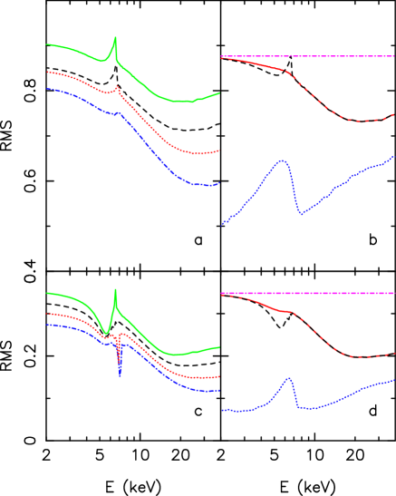
Figure 1: Panel (a) shows the RMS spectra for model $A$ with $h_{\rm s}$ changing between 1.8 and 10. Panel (c) shows the RMS spectra for model $C$ with $h_{\rm s}$ changing between 4 and 20. In both panels, the spectra from top to bottom are for $\theta_{\rm obs}=25\degr$ (solid, green online), $30\degr$ (dashed, black; shifted vertically by -0.02, for clarity), $40\degr$ (dotted, red; shifted vertically by -0.04) and $45\degr$ (dot-dashed, blue; shifted vertically by -0.06). Panels (b) and (d) show the RMS spectra for various spectral components in model A and C, respectively, with $\theta_{\rm obs}=30\degr$ and other parameters indicated for panels (a) and (c). The curves, from bottom to top, are for Compton reflected hump (dotted, blue; note that it does not include the Fe line), primary + Compton reflection (solid, red) and primary (power-law) component (dot-dashed, magenta). The dashed (black) curve is for the total emission, i.e. primary continuum + Compton reflection + Fe line.

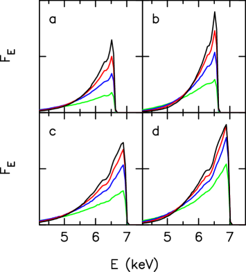
Figure 2: Changes of the Fe line profile in model $A$ (panels a and c) and model $C$ (panels b and d). The top panels are for $\theta_{\rm obs}=25\degr$; the bottom panels are for $\theta_{\rm obs}=40\degr$. In all panels, the profiles from bottom to top are for $h_{\rm s}=4$, 6, 8 and 10. Note that, for $\theta_{\rm obs}=40\degr$, rather subtle differences around the maximum of the blue peaks lead to opposite properties, i.e. a sharp excess or a sharp drop, around 6.9 keV in the RMS spectra for model $A$ and $C$, respectively, see Fig. 1. The units are arbitrary but the same in all panels; profiles in panels (a) and (b) are rescaled by a factor of 0.55.

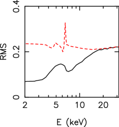
Figure 3: RMS spectra in two regimes where the fractional variability does not decline with increasing energy. The bottom (solid, black online) is for model C with $h_{\rm s}$ changing between 0.2 and 1.2. Only in this range of parameters is the reflected radiation more variable than the primary emission and a pronounced feature, related to the varying shape of the Fe edge, occurs in the RMS spectrum. The upper (dashed, red) is for model S with $r_{\rm s}$ changing between 6 and 12. Both spectra are for $\theta_{\rm obs}=30\degr$.

3 Results

Figures 1, 3, 4 and 5 show the RMS spectra for models $A$, $C$ and $S$, derived under the assumption that each of the individual spectra, $f_{i}(E)$, contributing to the RMS spectrum corresponds to a fixed, single position of a primary (point) source. The RMS spectra are computed for a constant intrinsic luminosity of the primary source. Figures 6 and 7 show the RMS spectra for more complex scenarios, discussed in Sects. 3.4 and 3.5.

3.1 Changes of $h_{\rm s}$

As shown in Figs. 1(a)(c) and 3, models assuming a vertical motion of the primary source do not predict a depression around 6.5 keV, similar to that revealed in MCG–6-30-15 (cf. Fig. 8 below). Moreover, an opposite property, i.e. increase of fractional variability at this energy, is typically predicted by these models in most of the parameter space. Before discussing the specific models, we comment on the generic impact of various spectral components on formation of the fractional variability spectrum, illustrated in Fig. 1(b)(d). The narrow excesses in the RMS spectra result from changes of the Fe line profile. These are investigated in detail in NZ08; here we briefly discuss some basic properties crucial for this study. We point out that relativistic distortions of the Compton hump are not as crucial for the fractional variability as distortions of discrete spectral features. This property results from a continuous energy distribution of the hump and, in most cases, leads to decrease of the RMS spectrum, consistent with observations.

The primary continuum is the most variable component, regarding variations of the directly observed flux, but it does not change the spectral shape. Then, its variability is represented by a flat RMS spectrum with a large amplitude. In turn, changes of the amount of primary radiation illuminating the disc - resulting from the change of $h_{\rm s}$ - are smaller (as a result of light bending). However, the distance of the most intensely illuminated area of the disc changes with $h_{\rm s}$. As a result, discrete spectral features in the reflected radiation, in particular the Fe K$\alpha$ line and edge, are subject to varying relativistic distortions, yielding an excess fractional variability around their rest energies. An excess, related to the variability of the blue peak of the Fe K$\alpha$ line, is seen in most of the spectra in Fig. 1(a)(c) (except for model $C$ with large $\theta_{\rm obs}$, see below). As we noted before, the excess variability caused by the Fe K$\alpha$ line occurs even when the total flux in the line does not change significantly.

Similarly, changes of the shape of the Fe K$\alpha$ edge result in a pronounced excess, around 7 keV, in the RMS spectra for the Compton reflected component, see the bottom curves in Fig.  1(b)(d). However, variability at this energy is dominated by the primary continuum and the Fe line, and the excess (due to the Fe edge) does not yield any significant signature in the RMS spectrum for the total observed radiation (except for model $C$ with small $h_{\rm s}$, see below). Crucially, though, for interpretation of the observed data, the distortions of the Fe edge yield a smooth RMS spectrum, see the middle solid curves, for the sum of the primary continuum and the Compton reflected radiation, in Fig. 1(b)(d), unlike the case of reflection from a static slab, for which a sharp drop occurs at 7.1 keV (cf Fig. 8 below).

The Compton hump, although subject to the same relativistic distortions as the Fe line, is less significantly affected by their changing amount, owing to the continuous spectral distribution of the hump. As a result, the amplitude of the RMS spectrum for the Compton reflected component is typically much smaller than for the primary emission, compare the top and bottom curves in Figs.  1(b)(d). As the contribution of the Compton reflected radiation to the total spectrum increases between 2 and 30 keV, the RMS spectrum for the total emission decreases, reaching a minimum around 30 keV where the reflection hump peaks.

3.1.1 Model $A$: light-bending (to the center)

Trajectories of photons emitted from a source located close to the symmetry axis are subject to a simple bending to the center, independent of the value of $a$ (contrary to bending to the equatorial plane, discussed in Sect. 3.3). Models involving a vertically moving source close to the axis predict strong variations of the observed flux. They result from changing amounts of purely GR effects, i.e. the light bending and gravitational time delay. However, these models robustly predict an enhanced variability around the Fe K$\alpha$ energy, see Fig. 1(a). This property, inconsistent with observations, property results from the fact that a source located at a larger $h_{\rm s}$ illuminates a more extended area of the disc and, therefore, the increase of $h_{\rm s}$ gives rise to rather significant strengthening of the blue peak (see Fig. 2a). The varying strength of the peak yields a pronounced excess in the RMS spectrum between 6 and 7 keV.

Dependence on $\theta_{\rm obs}$, seen in Fig. 1(a), results from gravitational focusing and Doppler collimation, toward observers with high inclination angles, of radiation reflected from the innermost parts of the disc (which receive most of irradiating flux from a source located at small $h_{\rm s}$). A stronger contribution of the Compton reflected radiation for larger $\theta_{\rm obs}$ gives rise to a stronger decrease of the RMS spectra with increasing energy. The focusing toward higher $\theta_{\rm obs}$ results also in weaker variations of the blue peak (compare Figs. 2(a) and 2(b)) and, thus, in a less pronounced RMS excess around 6.4 keV.

3.1.2 Model $C$: azimuthal motion

The major difference between models $A$ and $C$ results from rotation of the primary source around the symmetry axis in the latter model. Then, in model $C$, changes in the fluxes of the directly observed and the irradiating radiation, induced by the change of $h_{\rm s}$, result from the combination of light bending and Doppler beaming related to this motion (we recall that in both models $A$ and $C$ the intrinsic luminosity remains constant). The specific kinematic assumptions of model $C$ yield a non-monotonic dependence of azimuthal velocity on $h_{\rm s}$, leading to different properties of the model in two ranges of $h_{\rm s}$ (see NZ08 for details). The critical height, approximately limiting these two ranges, is the one at which the azimuthal velocity achieves a maximum value (for $\rho_{\rm s}=2$ this maximum occurs at $h_{\rm s}=2$). At small $h_{\rm s}$ ($<2$ for $\rho_{\rm s}=2$), variations of the directly observed primary continuum are strongly reduced and the RMS spectrum is shaped by spectral changes of the Compton hump; note that the reduced variations of the primary flux are observed only at smaller $\theta_{\rm obs}$ (i.e. these considered here) and result from more efficient Doppler beaming to larger $\theta_{\rm obs}$, due to the increase of $v_{\rm s}^{\phi}$, which approximately balances less efficient light bending with the increase of $h_{\rm s}$. The predicted increase of the RMS variability for increasing energies, accompanied by excess variability around 6 keV (caused by the changing Fe K$\alpha$ edge), see Fig.  3, is clearly not consistent with observed data.

At larger heights, the trends in both components are reversed. The primary continuum is now the most variable component, yielding the decrease of the RMS spectrum towards higher energies. Effects related to changes of the line profile strongly depend on $\theta_{\rm obs}$. The crucial property resulting from the Doppler beaming of primary emission is that the reflected radiation originates from more extended regions of the disc (with $r>h_{\rm s}$, as opposed to model $A$) and hence the Fe line is somewhat less variable than in model $A$ (see Fig. 2). This is reflected in the RMS spectrum by the sharp drop, with the width of a few hundred eV, occurring for $\theta_{\rm obs}>30\degr$ at the energy of the maximum of the blue peak. Regardless of the value of $\theta_{\rm obs}$, model $C$ predicts a pronounced depression around 5.5 keV.

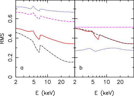
Figure 4: Panel (a) shows the RMS spectra for model $S^{\rm NZ}$ with different values of spin parameter $a=0.9$ (dotted, blue online), 0.95 (dashed, magenta), 0.98 (solid, red) and 0.998 (dot-dashed, black), from top to bottom. For all curves, $r_{\rm s}$ varies between $r_{\rm min}=r_{\rm ms}(a)$ and $r_{\rm max}=3.2$, and $\theta_{\rm obs}=30\degr$. Panel (b) shows the RMS spectra for various spectral components, as in Fig. 1(b)(d), in the model with $a=0.98$.

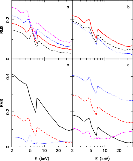
Figure 5: Dependence of the RMS spectra in model $S^{\rm NZ}$ on: $\theta_{\rm obs}$ (a); $\theta_{\rm s}$, or equivalently $h_{\rm s}/r_{\rm s}$ (b); $r_{\rm min}$ and $r_{\rm max}$ (c); $\beta$ (d). All spectra are for $a=0.998$; panels (b-d) are for $\theta_{\rm obs}=30\degr$; panels (a),(b) and (d) are for $r_{\rm min}=2$ and $r_{\rm max}=3$. Panel (a): $\theta_{\rm obs}=25\degr$ (dot-dashed, magenta online; shifted vertically by 0.06), $30\degr$ (dotted, blue; shifted by 0.04), $40\degr$ (solid, red; shifted by 0.02) and $45\degr$ (dashed, black). Panel (b): the spectra from top to bottom are for $h_{\rm s}/r_{\rm s}=0.07$ (solid, red; shifted vertically by 0.04), $h_{\rm s}/r_{\rm s}=0.14$ (dashed, black; shifted vertically by 0.02) and $h_{\rm s}/r_{\rm s}=0.21$ (dotted, blue). Panel (c): the spectra from top to bottom are for $r_{\rm s}$ varying between $r_{\rm min}=1.6$ and $r_{\rm max}=2.6$ (solid, black), $r_{\rm min}=2$ and $r_{\rm max}=3$ (dashed, red), $r_{\rm min}=2.4$ and $r_{\rm max}=3.4$ (dotted, blue). Panel (d): the spectra from top to bottom are for $\beta=2$ (dotted, blue), $\beta=1$ (dashed, red), $\beta=0$ (solid, black), $\beta=-0.7$ (dot-dashed, magenta).

3.2 Model $S$, large $r_{\rm s}$: local Doppler effects

The upper curve in Fig. 3 shows the RMS spectrum for model $S$ with large $r_{\rm s}$ ($\geq 6$). Radiation reprocessed from the emission of a source located close to the disc surface at large $r_{\rm s}$ originates in bulk from a small spot below the source. In such a case, both the directly observed primary emission and the reflected radiation are subject to the same relativistic distortions and, therefore, the relative normalization of the latter component is the same as for a static slab illuminated in flat space-time. The departure of the RMS spectrum from a flat form results from varying Doppler distortion of the Fe line, corresponding to changes of $r_{\rm s}$. These changes yield a strong excess around 6.4 keV due to the change of the energy of the maximum of the blue peak. An additional, smaller excess related to the varying extent of the line occurs at lower energies.

Note, however, that such a strong excess corresponds only to a simplified scenario with $n_{X}=1$ (see Sect. 3.4).

3.3 Model $S^{\rm NZ}$ (small $r_{\rm s}$ in the Kerr metric): bending to the equatorial plane

Figures 4 and 5 show the RMS spectra for model $S^{\rm NZ}$ with small, varying $r_{\rm s}$ and large $a$. Such parameters define a unique regime with the reduced variability of the blue peak of the line occurring independently of other specific assumptions. In this scenario, the reflected radiation has two components with different variability behavior. The first one arises locally from a strongly irradiated spot (or - after azimuthal averaging - a narrow ring) under the primary source. In principle, this component follows the behavior described in Sect. 3.2, but - in addition - it is subject to strong (and varying with $r_{\rm s}$) gravitational redshift. The variable redshift of the Fe line gives rise to a pronounced excess in the RMS spectrum between 4 and 6 keV. The second component arises from a slightly more distant region, at $\sim 10R_{\rm g}$, which is strongly illuminated due to bending to the equatorial plane, an effect significantly affecting radiation emitted from $r_{\rm s}<4$ for $a>0.9$. It is the second component which yields the unique properties of this model, through the combination of the following two effects: (1) the observed blue peak is formed mostly by photons emitted at $\sim 10R_{\rm g}$; and (2) the flux illuminating that site remains approximately constant while $r_{\rm s}$ changes (see NZ08 for details). The resulting reduction of variations of the blue peak yields a pronounced depression in the RMS spectrum between 6 and 7 keV. As the reduction effect fully relies on the properties of the Kerr metric, it is obviously stronger for larger $a$, see Fig. 4(a).

Similarly to model $A$ and model $C$ with $h_{\rm s}>2$, the Compton component is less variable than the primary continuum, see Fig. 4(b), and as a result the RMS spectrum decreases with increasing energy.

The most significant change in the RMS spectrum, corresponding to the change of $\theta_{\rm obs}$, is related to the shape and location of the excess between 4 and 6 keV (produced by variations of the red wing), see Fig. 5(a). Similarly, the change of $\theta_{\rm s}$ is most significantly reflected in the shape of the excess. For smaller $\theta_{\rm s}$, i.e. larger $h_{\rm s}/r_{\rm s}$, the hot spot under the source, where the variable part of the red wing is formed, is more extended and therefore the excess is less pronounced, see Fig. 5(b).

In model $S^{\rm NZ}$, the RMS spectrum is extremely sensitive to even small changes in $r_{\rm min}$ and $r_{\rm max}$, see Fig. 5(c). For $r_{\rm min}\geq 2.4$, bending to the equatorial plane is too weak to give rise to a significant reflection component from larger $r$ and the RMS is flat above 6 keV.

Figure 5(d) illustrates changes of the RMS spectrum resulting from the change of the radial profile of intrinsic luminosity, with the power-law modification parametrized by $\beta$, defined in Sect. 2.2. Interestingly, less centrally concentrated profiles, with $\beta>0$, preserve the shape of the RMS spectrum with only a slight change in the shape of the excess between 4 and 6; however, the amplitude of the spectrum increases significantly with the increase of $\beta$. For $\beta<0$, the RMS spectra flatten; furthermore, for $\beta<-0.5$ their qualitative properties change, see the dot-dashed curve. In particular, no drop around 6.4 keV occurs, and the spectrum increases at $E>10$ keV. Note that such negative values of $\beta$ would characterise discs with non-zero stress at the marginally stable orbit, considered e.g. by Krolik (1999).

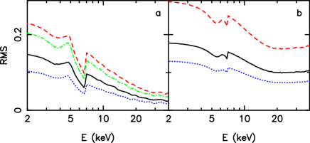
Figure 6: Changes in the RMS spectrum corresponding to the increase of the number, $n_{\rm X}$, of the source positions contributing to the energy spectra. Panel (a): model $S^{\rm NZ}$ with $\delta=0$, $r_{\rm min}=1.8$ and $r_{\rm max}=3$. Panel (b): model $C$ with $h_{\rm min}=4$ and $h_{\rm max}=20$. Models in both panels assume $a=0.998$ and $\theta_{\rm obs}=35\degr$. In both panels, the dashed (red online), solid (black) and dotted (blue) curves correspond to $n_{\rm X}=1$, 3 and 5, respectively. The dot-dashed (green) curve in panel (a) is for a single ($n_{\rm X}=1$) primary source with the size $\Delta r_{\rm s}=0.2$.

3.4 More complex arrangements of the primary source

We consider here the RMS spectra constructed from the energy spectra, $f_{i}$, formed by contributions from several positions of the source. A model with compact flares occurring simultaneously at various random locations is an obvious example requiring such treatment. An equivalent effect should occur, regardless of the configuration of the emitting region, in any model involving changes of location, for the increase of the size of time bins.

The energy spectra in this (and the following) section are computed as a mixture of spectra from randomly generated positions. In Fig. 6 the positions are drawn with uniform probability and in Fig. 7(a) we illustrate the effects of the change of the probability distribution.

Figures 6(a)(b) show changes in the RMS spectra resulting from the increase of the number of source positions, $n_{X}$, contributing to an individual spectrum, $f_{i}$. Obviously, deviation between the average spectrum and each of the individual spectra decreases, with the increase of $n_{X}$, which reduces both the RMS amplitude and the dependence of the RMS spectrum on energy.

An essentially similar, but less pronounced, effect occurs for an increase of the size, $\Delta r_{\rm s}$, of the primary source, see the dot-dashed curve in Fig. 6(a); emission of an extended source is approximated by superposition of emissions from point sources located in the range [$r_{\rm s}-0.5\Delta r_{\rm s}$, $r_{\rm s}+0.5\Delta r_{\rm s}$], so the energy spectra for $\Delta r_{\rm s}=0.2$ are formed by adding spectra from 3 adjacent positions of the model $S^{\rm NZ}$ grid. Again, deviations between spectra from more extended primary sources are smaller than in models with a single point source. However, differences between spectra are more systematic, and larger, than between those resulting from $n_{\rm X}>1$ with randomly generated $r_{\rm s}$ and, therefore, the flattening effect is weaker.

Note that the change of the radial probability density (which effectively modulates the radial emissivity profile) has a different effect on the RMS spectrum than the change of the radial luminosity profile. In particular, the dominating contribution from smaller $r_{\rm s}$ (corresponding to $\delta<0$) does not result in a qualitative change of the RMS spectrum (contrary to the modification with $\beta<0$), see Fig.  7(a).

Our model for the generation of active regions, with the same number of source locations contributing to each spectrum, and an implicit assumption of the same duration of emission at each position of the source, is certainly oversimplified; see e.g. Pecháček et al. (2008) for a more sophisticated modeling of the generation of flare-like features in random processes. Our main purpose here is to illustrate flattening of the RMS spectrum, which is a generic trend corresponding to the increase of $n_{X}$. See also Czerny et al. (2004) for the RMS spectra from their model of a spotted disc, which are much flatter than those made here with small $n_{X}$ (however, their model neglects effects of transfer from the X-ray source to the disc, which is a qualitative difference to our model $S^{\rm NZ}$).

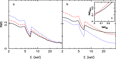
Figure 7: Panels (a) and (b) are for model $S^{\rm NZ}$ with $\theta_{\rm obs}=35\degr$, $a=0.998$, $r_{\rm min}=1.8$, $r_{\rm max}=3$ and $n_{\rm X}=1$. Panel (a): the spectra from top to bottom are for $\delta=-1.5$ (dotted, blue online), $\delta=0$ (dashed, red) and $\delta=1.5$ (solid, black). Panel (b): The dotted (blue) curve is for constant intrinsic luminosity, $L^{\rm PT}(r_{\rm s})$, at given $r_{\rm s}$; the solid (black) curve is for intrinsic luminosity generated from the Gaussian distribution with $\sigma_{\rm L}(r_{\rm s})=0.15L^{\rm PT}(r_{\rm s})$; the dashed (red) curve is for intrinsic luminosity generated from a uniform distribution with $s=0.15$. The inner panel (c) shows the RMS amplitude in a model involving changes of intrinsic luminosity as a function of the RMS variability without such changes; the dashed (red) and the solid (black) curves are for the uniform and Gaussian distribution, respectively, both with $s=0.15$; see text for details.

3.5 Changes of intrinsic luminosity

Finally, we take into account changes (in time) of intrinsic luminosity. The ability to describe the entire variability pattern in terms of relativistic effects is an attractive property of GR models, however, assumption of a strictly constant luminosity seems rather unrealistic. Results of the previous sections, though, could be applied directly to modeling a system with the time-scale of intrinsic variations much shorter than the time-bin length (so that each bin probes emission averaged over various luminosity states).

Figure 7(b) shows the RMS spectra for model $S^{\rm NZ}$, combining changes of the radial location with changes of the intrinsic luminosity (at each given $r_{\rm s}$). The location $r_{\rm s}$ is randomly generated (with $\delta=0$) and for each $r_{\rm s}$ we generate a random value of luminosity. Thus, the generated sequence of basic energy spectra typically contains several contributions from a given location, each with a different normalization.

It is interesting to notice that the results depend on the assumed distribution of luminosities. In order to illustrate this, we construct the RMS spectrum using:

(i) a Gaussian distribution, $P(L)\propto\exp[-0.5(L-L_{0})^{2}/\sigma_{\rm L}^{2}]$, where $L_{0}=L^{\rm PT}(r_{\rm s})$ and $\sigma_{\rm L}=sL^{\rm PT}(r_{\rm s})$;

(ii) a uniform distribution in the range $[L_{0}(1-s),L_{0}(1+s)]$, with $L_{0}=L^{\rm PT}(r_{\rm s})$.

In both cases, $s$ is a constant number (independent of $r_{\rm s}$), thus, both the deviation for distribution (i) and the amplitude of variations for distribution (ii) change slightly with $r_{\rm s}$. In general, changes of intrinsic luminosity increase the amplitude of the RMS spectrum, however, the Gaussian distribution leads also to flattening, while the uniform distribution does not change the shape of this spectrum with respect to that from the model with constant luminosity.

The relevant property underlying the above difference is illustrated in Fig. 7(c). The figure shows the relation between the RMS computed with (${\rm RMS}_{\rm GR+L}$) and without (${\rm RMS}_{\rm GR}$) changes of intrinsic luminosity for a simple model using two random quantities, $x_{F}$ and $x_{L}$. $x_{F}$ is generated using a uniform distribution and represents the received flux in GR models with constant luminosity. $x_{L}$ represents the intrinsic luminosity and is generated using a Gaussian (the solid curve) or uniform (the dashed curve) distribution, as defined above, both with $s=0.15$. ${\rm RMS}_{\rm GR}$ is constructed using the generated values of $x_{F}$, the increase of the amplitude of variations of $x_{F}$ yields larger ${\rm RMS}_{\rm GR}$. ${\rm RMS}_{\rm GR+L}$ is constructed using the products of $x_{F}$ and $x_{L}$. Note that the uniform distribution of $x_{L}$ leads to a linear relation between ${\rm RMS}_{\rm GR+L}$ and ${\rm RMS}_{\rm GR}$, which is reflected in the unchanged shape of the spectrum in Fig. 7(b), while for the Gaussian distribution this relation flattens at small ${\rm RMS}_{\rm GR}$.

4 Application to MCG–6-30-15

4.1 The Suzaku observations

Because of the wide bandpass coverage of energies provided by detectors on-board Suzaku, it is currently the most suitable X-ray observatory for testing relativistic reflection models. In particular, crucial information comes from the Hard X-ray Detector data, allowing us to measure the Compton reflection hump simultaneously with the Fe K$\alpha$ line. MCG–6-30-15 was observed three times by Suzaku in 2006 January in a state typical for this source, regarding the mean X-ray flux and variations of the flux by a factor of $\sim 2$ in a few ksec (see Miniutti et al. 2007). Crucially for our analysis, Miniutti et al. (2007) find for these observations that (1) the average profile of the Fe K$\alpha$ line has a relativistic shape, with the pronounced blue peak and the red wing extending down to $\simeq 4$ keV, consistent with that from the long XMM observation in 2001 (Fabian et al. 2002); (2) the average relative normalization of the Compton hump, given by the usual parameter $R$ ($R=1$ corresponds to the strength of reflection expected from a reflector subtending $2\pi$ sr at an isotropic primary source), is $R\simeq 3.8$, consistent with previous estimations from Beppo-SAX (Ballantyne et al. 2003), and rises to $R\approx 5$ in the low flux spectra; (3) on a time-scale of tens of ksec, spectral changes are consistent with the phenomenological, two-component model.

We use the data from three observations of MCG–6-30-15 by the Suzaku satellite on 2006 January 9–14 (143 ksec exposure), 23–26 (99 ksec) and 27–30 (97 ksec). The total on-orbit time is about 780 ksec. For data reduction, we have used the HEADAS 6.5 software package provided by NASA/GSFC. We determined the RMS amplitude, and its error, as a function of energy, in the standard manner (e.g. Vaughan et al. 2003b; the definition is analogous to equation (3) but contains an additional term related to the count rate error). In this paper we use the RMS spectra for two time-bin sizes, approximately 16 ksec and 131 ksec (more specifically $2^{14}$ sec and $2^{17}$ sec), with approximately 7 and 50 ksec of exposure time per bin, respectively. The RMS spectra for 16 ksec and 131 ksec are shown in Fig. 8(b) and all panels of Fig. 9 by the upper and lower set of points, respectively.

The RMS spectra indicate strong decrease of variability at $<1$ keV, however, modeling of this band is beyond the scope of this paper. The decrease most likely results from the presence of a soft X-ray excess, which is clearly seen in the average spectra of MCG–6-30-15 as well as in the spectrum of the non-varying spectral component (see e.g. figs. 3 and 22 in Vaughan & Fabian 2004). The origin of such soft excesses, typically observed in AGNs, is not clear (see e.g. Sobolewska & Done 2007). Remarkably, one of the possible explanations, involving the relativistically blurred photoionized disc reflection (where the soft excess is explained as being composed of many broad lines, see Crummy et al. 2006), is consistent with the scenario discussed in Sect. 5.5.

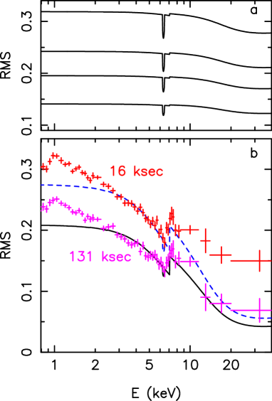
Figure 8: All curves show the RMS spectra for a model with a constant Compton reflection (derived with pexrav), a constant line at 6.4 keV with EW = 30 eV (and with $\sigma=0.1$ keV, matching the width of the data energy bin) and a varying power-law component. Panel a: the RMS spectra are computed with various amplitudes of the power-law variability, but all have the same $R=0.15$, approximately consistent with the EW of the line. Panel b: the simulated RMS spectra, with $R=4$, compared with the Suzaku data. The upper (red) and lower (magenta) points show the RMS spectra for the Suzaku observations with a time bin size of 16 ksec and 131 ksec, respectively.

4.2 Non-relativistic reflection

Before applying the GR models, we briefly comment on the contribution of reflection from distant matter, which for some other objects is considered as the explanation for RMS spectra similar to these derived in MCG–6-30-15 (e.g. Terashima et al. 2009). In MCG–6-30-15, however, such a component should have a marginal effect, as indicated by the very small contribution of a narrow Fe K$\alpha$ line at 6.4 keV (e.g. Iwasawa et al. 1996; Lee et al. 2002).

For the Suzaku observation, the equivalent width (EW) of the narrow 6.4 keV line is approximately 30 eV (Miniutti et al. 2007), suggesting that the distant reflector subtends a small solid angle at the central X-ray source with $R=0.15$ being a likely value characterising the strength of the accompanying reflection hump. In Fig. 8a, we show the RMS spectra for a simple non-relativistic model involving a variable power-law and a constant reflection component with $R=0.15$ and a narrow Fe K$\alpha$ line with EW=30 eV (both EW and $R$ are determined with respect to the average power-law component). The RMS spectra are computed for various levels of variation of the power-law continuum; the index, $\Gamma$, of the power-law remains constant while its intensity changes. The reflection spectrum is derived using the pexrav model, with the inclination angle of the reflector fixed at $30\degr$. The constant line at 6.4 keV is computed with a rather large width, $\sigma=0.1$ keV, for a clear comparison with the observed RMS spectra (which are derived with the energy bins $\Delta E=0.2$ keV around 6.5 keV). The constant line at 6.4 keV, with ${\rm EW}=30$ eV and $\sigma=0.1$ keV, is also included in all models in Figs. 8(b), 9 and 10.

For a constant spectral component, with the fixed contribution to the average spectrum, the strength of the related signature in the RMS spectrum depends on the overall level of variability. For ${\rm RMS}=0.3$, both a constant hump with $R=0.15$ and a line with ${\rm EW}=30$ eV would lead to rather pronounced declines in the RMS spectrum (see the top curve in Fig. 8a). However, if another spectral component dilutes the variability, as should be the case in MCG–6-30-15, the strength of these declines decreases. Specifically, ${\rm RMS}=0.05$–0.15, derived from the data above 10 keV, makes the hump with $R=0.15$ negligible. For ${\rm RMS}=0.15$–0.2, as observed around 6 keV, the line with ${\rm EW}=30$ eV has a noticeable, but rather minor, effect.

The observed shape of the RMS spectrum can be approximately reproduced, above 3 keV, in a simple non-relativistic model, involving a constant reflection component with $R\ga 3$ (see Fig. 8b). Such an apparently unphysical (for reflection from a distant matter) value of $R$ could result from the effect of the light travel time in a source observed in low luminosity state (as for the Suzaku observation of NGC 4051; Terashima et al. 2009) or from GR effects affecting the primary emission. In the latter case, more relevant for MCG–6-30-15, the mechanism is similar to model $S^{\rm NZ}$. Namely, if generation of X-rays occurs within a few $R_{\rm g}$ from a rapidly rotating black hole, a face-on observer would directly receive reduced primary radiation, which would be strongly focused along the equatorial direction to the distant material, giving rise to a strong non-relativistic reflection component. In MCG–6-30-15 this scenario seems to be ruled out by the small EW of the narrow K$\alpha$ line. Moreover, modeling the RMS spectra for various time-bin sizes seems to require slightly different values of $R$ (approximately 3 and 4 for 16 ksec and 131 ksec, respectively), which is inconsistent with a simple reflection model (where $R$ should not depend on the time-bin size). As an illustration, the RMS spectra in Fig. 8(b) are computed with $R=4$. While the lower curve roughly matches the spectrum for 131 ksec, the upper curve strongly underpredicts the variability above 10 keV, as compared to the spectrum for 16 ksec.

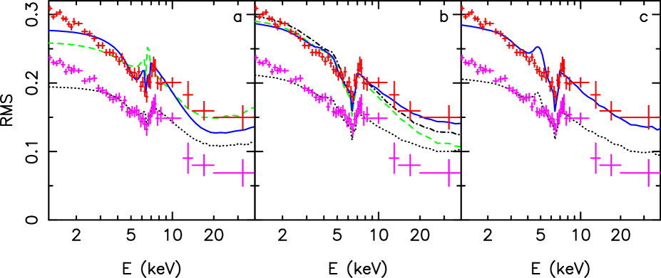
Figure 9: Fits of the Suzaku RMS spectra with the GR models. In all panels, the upper (red online) and lower (magenta) points show the Suzaku RMS spectra for 16 ksec and 131 ksec, respectively. All models involve a constant line at 6.4 keV with the ${\rm EW}=30$ eV and $\sigma=0.1$ keV; all models assume $a=0.998$ and $\theta_{\rm obs}=35\degr$. Panel (a): models involving vertical motion of the primary source. The dashed (green online; shifted vertically by $-0.4$) curve is for model $A$ with $h_{\rm min}=2.2$ and $h_{\rm max}=10$. The solid (blue; shifted vertically by $-0.07$) and dotted (black; shifted vertically by $0.01$) curves are for model $C$, with $h_{\rm min}=4$ and $h_{\rm max}=20$, for $n_{\rm X}=1$ and 3, respectively. Panel (b): the solid (blue) and dotted (black) curves are for $n_{\rm X}=3$ and 5, respectively, in model $S^{\rm NZ}$ with $r_{\rm min}=1.6$, $r_{\rm max}=3$, $\delta=-1.5$, $\sigma_{\rm L}=0.2L^{\rm PT}$ (and $\beta=0$). The dot-dashed (black) curve is for the same parameters as the solid curve, except for (larger) $r_{\rm max}=3.4$. The dashed (green) curve is for $r_{\rm min}=1.4$ and $r_{\rm max}=3$; $n_{\rm X}=3$, $\beta=0$, $\delta=0$, $\sigma_{g}=0$. Panel (c): model $S^{\rm NZ}$ with $r_{\rm min}=1.8$ and $r_{\rm max}=3$, $\beta=1$ ($\delta=0$ and $\sigma_{\rm L}=0$); $n_{\rm X}=2$ and 3 for the solid (blue) and dotted (black) curve, respectively.

4.3 GR models

The RMS spectra predicted by the GR models for some ranges of parameters are qualitatively inconsistent with those observed, as discussed in Sect. 3. Thus, the observed data completely rule out model $A$ (for completeness of our discussion, the best fit with this model is presented in Sect. 4.3.1), model $S$ with $r_{\rm s}>4$ and model $C$ with $h_{\rm s}<2$, cf. Figs. 1 and 3.

Some details of the RMS spectra in the GR models are sensitive to the value of $\theta_{\rm obs}$. In our analysis we consider the inclination angles between $\theta_{\rm obs}=25\degr$ and $45\degr$. We recall that the disc-line fits to the ASCA observations of MCG–6-30-15, in which the line seems to extend only up to $\simeq 6.8$ keV, yield $\theta_{\rm obs}\simeq 30\degr$. However, higher quality data indicate that the line extends beyond $7$ keV (but is indented by two absorption edges) and recent fits to both the XMM (Larsson et al. 2007) and Suzaku (Miniutti et al. 2007) observations indicate a larger value, $\theta_{\rm obs}\simeq 40\degr$.

In models $A$ and $C$ we adjusted the amplitude of the RMS spectra to match the observed data, which is the usual procedure in spectral modeling. In model $S^{\rm NZ}$ we did not treat the amplitude as a free parameter. Instead, we attempted to reproduce self-consistently both the shape and the amplitude of the RMS spectrum by modifying the auxiliary parameters of the model, i.e., $\sigma_{\rm L}$ and $\delta$ or $\beta$.

The model spectra best fitting the data are shown in Fig. 9. Our formally best fitting case, shown by the solid curve in Fig. 9(b) has the (reduced) $\chi_{\nu}^{2}\approx 2$ (with 24 d.o.f.) for $E>3$ keV; the remaining fits in Fig. 9 yield $\chi_{\nu}^{2}>3$. Clearly, the fits are not acceptable statistically. On the other hand, the basic trends are reproduced by model $S^{\rm NZ}$ reasonably well and we suspect that the quality of the fits could be improved when additional physical effects, neglected in this paper (e.g. ionization), are taken into account.

A further indication of the incompleteness of our models is given by the systematic discrepancies below 4 keV. Between 2 and 4 keV, the RMS spectra predicted by the GR models are typically more convex than these observed, similarly to the case of non-relativistic models (cf. Fig. 8b). Only model $S^{\rm NZ}$ with $r_{\rm min}<2$ (producing a strongly redshifted reflection component), yields the RMS spectra with approximate agreement down to 2 keV.

Studies of strong gravity effects in the time-averaged spectrum of MCG–6-30-15 usually concentrate on the data above 3 keV, as the spectrum at lower energies is strongly affected by a warm absorber (while at larger energies the absorption effects are considered to be unimportant; see e.g. Miniutti et al. 2007). We also do not attempt to model the RMS spectra below 3 keV, as changes of the absorber may determine variability in this band. On the other hand, some controversies remain as to whether the absorber does exhibit strong changes, see Sect. 5.6, and we point out that a weakly varying absorption should not affect the RMS variability significantly. Considering the lack of absorber variability suggested by some previous studies, we note that the deficiency of GR models below 3 keV results from the small contribution to the total spectrum of the radiation reflected from neutral matter at these energies. Then, ionization of the innermost parts of the disc (which is most likely in model $S^{\rm NZ}$, see Sect. 5.5) may be relevant to extend these models to lower energies.

4.3.1 Models $A$, $C$

In models $A$ and $C$ we considered $h_{\rm s}\leq 20$. We were not able to find the RMS spectra matching both the shape and the normalization of those observed. Then, we focused on reproducing the shape of the RMS spectrum and we adjusted the amplitude, which is treated as a free parameter only in this section. We presume that moderate changes of the RMS normalization could result from a departure from the (vertically constant) distribution of the intrinsic luminosity assumed in these models. In general, the model RMS spectra with a (qualitatively) consistent shape have larger normalization than those observed, therefore, we neglected variations of intrinsic luminosity in time, which would lead to a further increase of the RMS amplitude.

The dashed curve in Fig. 9(a) shows the RMS spectrum in model $A$, with $\theta_{\rm obs}=35\degr$, $h_{\rm min}=2.2$ and $h_{\rm max}=10$, best matching the observed shape; the model spectrum is shifted down by $\Delta{\rm RMS}=-0.4$. An excess variability in the energy range of the Fe K$\alpha$ line, robustly predicted by model $A$, is clearly inconsistent with the observed data. We do not expect that modifications of our model, specifically those related to ionization of the disc, could reduce this discrepancy (see Sect. 5.5) and thus we rule out this model. We also note that the observed level of the RMS variability can be achieved in model $A$ with $h_{\rm min}>3$, but in such a case the model RMS spectrum is much flatter than observed. On the other hand, the stronger contribution from small $h_{\rm s}$, e.g. for $h_{\rm min}<2.2$, yields a larger excess around 6.4 keV.

Model $C$ predicts, for $\theta_{\rm obs}>30\degr$, a sharp drop at the maximum of the blue peak, cf. Fig. 1(c), which cannot account for the observed, broader depression in 6–7 keV range. However, for $\theta_{\rm obs}=35\degr$, the drop occurs around 6.8 keV and including an additional narrow line at 6.4 keV we achieve an overall form of the depression between 6 and 7 keV which can imitate the observed one. Then, we found the set of parameters ($\theta_{\rm obs}=35\degr$, $h_{\rm min}=4$, $h_{\rm max}=20$; the solid curve in Fig. 9a) for which deviations between the predicted and observed shapes are small. The predicted RMS amplitude only slightly exceeds the observed value, the model spectrum is shifted down by $\Delta{\rm RMS}=-0.07$. The dotted curve in Fig. 9(a) illustrates the extrapolation of the model for larger time-bin sizes, obtained with $n_{X}>1$.

Model $C$ requires a fine-tuning of parameters to approximately explain the observed fractional variability. For the inclination angles higher or lower than $\theta_{\rm obs}=35\degr$, discrepancies around the energy of the Fe K$\alpha$ line are more significant. For the range of heights different to $h_{\rm s}\simeq 4$–20, the RMS spectrum between 3 and 20 keV is too flat. See Sect. 5.3 for a further, critical discussion of the fits with model $C$.

4.3.2 Model $S^{\rm NZ}$

Both the shape and amplitude of the observed RMS spectrum can be approximately reproduced with $a\geq 0.98$ and the distance of the primary source varying in the range extending down to at least $r_{\rm s}\approx 2$. For smaller spins, or larger distances, the model RMS spectrum is flatter than observed. Models with $n_{X}>1$ strongly favour the maximum value of $a=0.998$. The major challenge in modeling the observed RMS spectrum results from the excess related to changes of the red wing, which is not seen in the data. A strong ionization of the disc, at the site of the formation of the variable part of the red wing, may be relevant in reducing this discrepancy, see Sect. 5.4. In the simplest case (with, in particular, a neutral and untruncated disc) considered in this paper, fits with model $S^{\rm PT}$ favour $r_{\rm min}<2$, for which (1) the excess is more extended and less pronounced, making a relatively small deviation between the model and the data, and (2) the significant contribution from the smallest $r_{\rm s}$ allows us to reproduce the RMS spectra down to 2 keV.

We attempted to reproduce the RMS spectra for both 16 and 131 ksec with the same set of parameters, differing only by the value of $n_{\rm X}$. In our procedure, we first adjusted $r_{\rm min}$, $r_{\rm max}$, $n_{\rm X}$, $\delta$, $\sigma_{\rm L}$ and $\theta_{\rm obs}$ to fit the 16 ksec spectrum, then we computed the spectra for larger $n_{\rm X}$ and compared them to 131 ksec. The differences between the amplitudes of the RMS for consecutive $n_{\rm X}$ are rather large, which is most challenging in attempts to reproduce both time-bins simultaneously (as noted before, the underlying assumption of identical $n_{\rm X}$ for each time bin is most likely oversimplified).

Our best fits, with $a=0.998$, $\theta_{\rm obs}=35\degr$, $r_{\rm min}=1.6$, $r_{\rm max}=3$, $\sigma_{\rm L}=0.2L^{\rm PT}$, $\delta=-1.5$, $n_{\rm X}=3$ and 5 for 16 and 131 ksec, respectively, are shown in Fig. 9(b). Disregarding the excess variability of the red wing (with the plausible impact of ionization in mind) we can reproduce the observed RMS spectra for a broader range of parameters. Example fits, achieved using $\beta$ instead of $\sigma_{\rm L}$ and $\delta$, with $\theta_{\rm obs}=35\degr$, $r_{\rm min}=1.8$ and $r_{\rm max}=3$, $\beta=1$, $n_{\rm X}=2$ (for 16 ksec) and 3 (for 131 ksec) are shown in Fig. 9(c).

The statistical quality of the fits is poor, as noted above, therefore, the usual criterion for constraining the confidence limits in the model parameters, using the increase of $\chi^{2}$, seems inadequate. Qualitatively, $r_{\rm min}\simeq 2.2$ seems to be the upper limit for $r_{\rm min}$; for larger $r_{\rm min}$, the RMS spectrum is too flat, see the bottom curve in Fig. 5(c). Similarly, we can reject submaximal ($<0.98$) values of $a$, cf. Fig. 4(a). The model with $r_{\rm min}=1.6$ and $r_{\rm max}=3$ is slightly favored in our fits; Fig. 9(b) shows trends corresponding to the extention of this range. In general, models with $r_{\rm max}>3$ give a more significant excess with respect to the data below 5 keV, see the dot-dashed curve. In turn, for our best fit with $r_{\rm min}=1.4$, variability above 10 keV is slightly underpredicted; notably, this fit (the dashed curve) involves no modification of our basic $S^{\rm NZ}$ model, i.e. $\sigma_{\rm L}=0$, $\delta=0$ and $\beta=0$, so the intrinsic luminosity follows exactly $L^{\rm PT}$. See Sect. 5.4 for further discussion of $r_{\rm min}$ and $r_{\rm max}$.

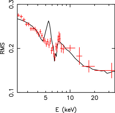
Figure 10: RMS spectrum for model $S^{\rm NZ}$ with an excess around 5.5 keV, as revealed by some previous observations (see text). Parameters $\beta=1.2$, $\delta=0$, $\sigma_{\rm L}=0$ and $n_{X}=1$ are adjusted to match the Suzaku RMS spectrum (for 16 ksec) at $E<5$ keV and $E>6$ keV.

4.3.3 Excess variability between 5 and 6 keV

As we discuss in Sect. 5.5, the excess variability of the red wing, which is the major prediction of model $S^{\rm NZ}$ ruled out by the Suzaku data, is likely to be reduced by ionization of the disc under the source. Interestingly, however, the RMS spectra from some previous observations of MCG–6-30-15 (see Matsumoto et al. 2003; Ponti et al. 2004) did reveal a strong enhancement of the RMS variability between 5 and 6 keV. Apart from this band, those RMS spectra are consistent with other observations of MCG–6-30-15. Presumably, the geometry of the X-ray emitting region does not change significantly between the various observations and the presence or lack of an excess is related to changing ionization state of the innermost disc.

Then, we examined conditions in which model $S^{\rm NZ}$ produces an excess between 5 and 6 keV but matches the Suzaku RMS spectra at other energies. An example of such an RMS spectrum for $\theta_{\rm obs}=40\degr$, $r_{\rm min}=2.2$ and $r_{\rm max}=3.2$ is shown in Fig.  10. We find that, in general, a relatively high inclination angle, $\simeq 40\degr-45\degr$, is required to explain the excess between 5 and 6 keV by a varying redshift of 6.4 keV photons – for smaller $\theta_{\rm obs}$ the excess occurs at lower energies.

The amplitude of the excess in Fig. 10 is approximately consistent with that found by Ponti et al. (2004) in the XMM data. However, we were not able to reproduce a stronger excess, with ${\rm RMS}\approx 0.4$, as reported by Matsumoto et al. (2003) for the ASCA observation. Such a strong excess can be explained by an enhanced contribution of Fe photons from the spot under the source, which could occur if ionization of that area of the disc is taken into account, namely, it could be attributed to intermediate stages of ionization (where Auger destruction cannot operate) giving rise to an intensity of the Fe photons much higher than from a neutral medium (e.g. Życki & Czerny 1994). For these ionization states, the rest energy of Fe photons is around 6.9 keV, and the range of inclination angle relevant to reproduce the excess would be $\theta_{\rm obs}\simeq 35\degr-40\degr$.

Interestingly, during the XMM observation analysed by Ponti et al. (2004), the source luminosity was $\sim 2$ times lower than the typical luminosity observed in MCG–6-30-15. This can support the above scenario, with the change from complete to intermediate ionization of a hot spot. In case of two ASCA observations used by Matsumoto et al. (2003) to reveal enhanced variability between 5 and 6 keV, the average luminosity was not much lower than typical, however, both observations contain prolonged deep minimum states, with the luminosity dropping to the lowest level observed in that object.

We point out that an excess between 5 and 6 keV cannot be produced by simple geometric effects in models $A$ or $C$; actually, the latter predicts an opposite property, i.e. reduced variability around 5.5 keV.

5 Summary and discussion

5.1 Conclusions

This paper focused on modeling the RMS spectra, which are commonly used to estimate the fractional variability amplitude in AGNs. We thoroughly studied the RMS spectra predicted by models relating spectral changes to varying amounts of GR effects, which distort the X-ray radiation generated in central parts of black-hole accretion flow. We applied our GR models to MCG–6-30-15 where the bulk of the reprocessed radiation is supposed to come from the inner accretion disc. Our main conclusions are summarized as follows:

(1) The Compton reflection hump, reprocessed in the accretion disc from the continuum emission generated at a small, varying distance from a black hole, is typically less variable than the primary continuum. This leads to a decrease of the RMS spectrum with increasing energy, above 3 keV (for neutral disc material). A remarkable exception involves a source corotating with the disc and changing height (as in the model of MF04) not far above the disc surface – in this case the fractional variability increases with energy.

(2) Relativistic distortions of the Fe K$\alpha$ line give rise to excess variability which is the major challenge in applications of GR models to observed data. In models involving vertical motion of the X-ray source, the excess variability, between 6 and 7 keV, is related to changes of the blue peak. In models involving changes of the radial distance, low above the disc surface, the excess is related to changes of the red wing and occurs between 4 and 6 keV. In the latter class of models, however, ionization of the hot spot under the source is very likely and should reduce the excess variability, see Sect. 5.5.

(3) The results of this paper illustrate the maximum strength of signals in the RMS spectra caused by the GR effects. Such strong signals could be observationally seen only in the RMS spectra determined with time-bin sizes not exceeding the time scale of the change of position of the X-ray source. For longer time bins, signatures of GR effects are weaker (i.e., the RMS spectra are flatter); some implications of this are discussed in Sect. 5.2.

(4) Variability observed in MCG–6-30-15 is inconsistent with models assuming vertical motion of the source. The model with a source on the symmetry axis is ruled out and the model by MF04 involving a specific pattern of rotation around the symmetry axis is disfavored as discussed in Sect. 5.3.

(5) The model with changes of the radial distance in the Kerr metric, proposed in NZ08, offers the most likely explanation of the observed properties (among the GR models); See Sect. 5.4 for further discussion of this model.

(6) Some details of the RMS spectra are sensitive to $\theta_{\rm obs}$, and they may provide constraints on inclination, independent of the modeling of the line profile. Interestingly, our GR fits to the RMS spectra from Suzaku observations of MCG–6-30-15 favor $\theta_{\rm obs}=35\degr-40\degr$, consistent with the disc-line fits to the Suzaku data. The light-bending (MF04) model requires exactly $\theta_{\rm obs}=35\degr$. The best fit with model $S^{\rm NZ}$ also has $\theta_{\rm obs}=35\degr$, however, this model allows for a broader range of $\theta_{\rm obs}$, especially when excess due to variability of the red wing is disregarded. The range of $\theta_{\rm obs}=35\degr-40\degr$ would also be relevant in reproducing the excess variability between 5 and 6 keV, which was reported for some previous ASCA and XMM observations, in a model involving a highly ionized hot spot under the hard X-ray source.

5.2 Variability time-scales

The energy spectra determined for increasing lengths of time-bins should consist of contributions from an increasing number of locations of the primary source. Then, the RMS spectra for longer time bins should be flatter, see Sect. 3.4. Below we briefly discuss the resulting implications for time-scales of various processes involved in generating the observed variability.

The reduced variations of the reprocessed component are typically assessed over $\ga 10$ ksec. We emphasize that the actual time-scale of the change of the position of the hard X-ray source should be at least of this order of magnitude, otherwise the RMS spectra would be much flatter than observed. Then, significant changes of the X-ray flux on a time-scale of $\sim 1$ ksec which are observed in MCG–6-30-15 should result from intrinsic variations (with small changes of geometry) of the hard X-ray source. The point-to-point RMS spectrum with 1 ksec time bins which measures such short time-scale variability, found to be much flatter than the standard RMS spectra in Vaughan & Fabian (2004), supports the scenario with changes of intrinsic luminosity dominating the short time-scale variability (by definition of the RMS spectrum, changes of luminosity, without the change of spectral shape, produce a flat RMS spectrum).

In Sect. 4.3.2 we note that the RMS spectra for both 16 ksec and 131 ksec can be reproduced with the same set of parameters, in a model involving a larger number of the source positions for the larger bin size. However, the number of positions in our fits for 131 ksec is only $\sim 2$ times larger than for 16 ksec, while a factor of 8 would be expected for a simple scaling of the number of positions with the bin length. Such a simple, linear scaling of the number of source locations is ruled out, as $\ga 10$ random locations, implied for 131 ksec, would yield an almost flat RMS spectrum. Then, the change of geometry on a time scale of $\sim 100$ ksec should obey some systematic pattern, involving at most a few localised regions dominating the total emission, with the duration of several tens of ksec. Emission averaged over the whole range of locations of the source is probably probed on a much longer time-scale, $>1000$ ksec, e.g. by the RMS spectra derived from long-term RXTE monitoring, see Markowitz et al. (2003), which are indeed flatter than these obtained with $10-100$ ksec bins.

Finally, note that the time-scales for the change of the source location, $\sim 10-100$ ksec, required by the above arguments are orders of magnitude longer than the dynamical time-scale for the innermost region, $\la 100$ sec, which is rather puzzling. On the other hand, the power-spectra indicate that most of the variability in MCG–6-30-15 indeed occurs on time scales $\geq 10$ ksec and a large-magnitude variability may extend even to time-scales longer than $100$ ksec (see Vaughan et al. 2003a; Uttley et al. 2002). Then, in the context of GR models, most of the power contained in the X-ray light curve of MCG–6-30-15 would result from changes of the geometry of the X-ray source. In turn, variability dominated by changes of intrinsic luminosity should correspond to frequencies higher than the break frequency ($10^{-4}$ Hz, above which the magnitude of variability drops).

5.3 Models involving vertical motion

Focusing of radiation produced close to the symmetry axis, toward the disc, cannot explain the detailed properties of MCG–6-30-15, despite qualitative arguments for the relevance of this mechanism. Significant changes of the blue peak corresponding to changes of the source height are the major cause of this model failure.

This discrepancy can be reduced in a modification of the model by MF04, where the observed RMS spectrum can be approximately reproduced with the height changing between $\simeq 4$ and $20R_{\rm g}$. We emphasize again that predictions of this light-bending model are related primarily to its specific kinematic assumptions rather than the light-bending itself. We disfavor this model on the grounds that it requires large elevations of the source above the disc, where the kinematic assumptions are rather arbitrary. At lower elevations (where the crucial assumption of this model – i.e. rotation of the source with $\Omega_{\rm K}(\rho_{\rm s})$, see Sect. 2.1 – has some physical motivation), the model predicts a variability pattern that is ruled out by observations. Even with the required range of $h_{\rm s}$, the model is rather unlikely as a decline of the fractional variability around 5.5 keV, systematically predicted by the model, has not been confirmed by any observation of MCG–6-30-15 (actually an opposite property has been reported, see Sect. 4.3.3). Another major shortcoming of this model was pointed out by NZ08. For the range of heights relevant to reproduce the observed variability ($\geq 4R_{\rm g}$), the model cannot explain the pronounced red wing of the relativistic Fe line, the feature that originally motivated the development of this model.

5.4 Model with bending to the equatorial plane

We strongly favor the model with radial motion in the Kerr metric for a description of the central region of MCG–6-30-15. Note that both of the main properties required by this model, i.e. rapid rotation of the black hole and very small distance of the X-ray source, have some independent support in the observed, time-averaged Fe line profile. Our condition for the value of the spin, $a>0.98$, is consistent with the formal constraint on the spin parameter, $a>0.987$ (Brenneman & Reynolds 2007), derived from the line profile under the assumption that the Fe photons are emitted only at distances larger than $r_{\rm ms}(a)$. Regarding the second condition (small distance), NZ08 point out that location of the X-ray source within a few central $R_{\rm g}$ is needed to explain the pronounced red wing of the line profile; the irradiation of the inner disc by a source located at further distances is too weak and the red wing is much weaker relative to the blue peak than in the observed profile.

In the relevant range of distances, the directly observed flux of primary X-rays is extremely sensitive to the location of the X-ray source, while the reflected radiation changes a little, and the observed variability effects can be reproduced by rather small changes in the geometry of the X-ray emitting region. The range of distances between approximately $1.6R_{\rm g}$ and $3R_{\rm g}$ is slightly preferred in our applications of this model to the Suzaku data. However, we emphasize again that some features of our model are oversimplified, most importantly our method for the generation of active regions and their luminosities as well as our neglect of ionization, and more realistic modeling could yield a more extended range of locations.

Remarkably, for $a=0.998$, the maximum of the dissipation rate given by the Page & Thorne (1974) formula occurs exactly at the lower end (i.e. $1.6R_{\rm g}$) of this range. Furthermore, according to that formula with $a=0.998$, $35$ per cent of the total power dissipated in a Keplerian disc is released within the central $3R_{\rm g}$. Then, our condition for the location of the hard X-ray source, although seemingly rather extreme, is not implausible.

An independent constraint on the range of distances comes from the normalization of the reflection component in the time-averaged spectrum. We have computed the reflection parameter, $R$, in our models as the ratio of the total fluxes in the reflected component in the GR model and in the pexrav model with the same flux of the primary power-law. Our fits with model $S^{\rm NZ}$, shown in Fig. 9, have $R\ga 4$, within the confidence limits, $R=3.8\pm 0.7$, found for Suzaku observations in Miniutti et al. (2007). A stronger contribution of primary hard X-rays from smaller radii (e.g. for $r_{\rm min}<1.6$, $r_{\rm max}=3$ and $\delta<0$) would yield, however, a larger value of $R$, inconsistent with the data.

In our investigation of the model we focused on the case with $h_{\rm s}/r_{\rm s}<0.1$. For $h_{\rm s}/R_{\rm s}\gg 1$, i.e. in the lamp-post regime, the bending to the center dominates over the bending to the equatorial plane, leading to qualitatively different effects, as described above. We did not investigate the case of intermediate $h_{\rm s}/r_{\rm s}$, as results in this regime strongly depend on (very uncertain) kinematic assumptions. Note that even for relatively small $h_{\rm s}/r_{\rm s}=0.2$, the difference between the azimuthal velocities resulting from the different assumptions discussed in Sect. 2.1 exceeds $0.1c$.

Note that occasionally an additional source of primary X-ray emission may be present in MCG–6-30-15, which would lead to a more complex temporal behaviour than estimated in this paper. Flaring releases of a part of the X-ray emission may occur at rather large heights ($>100R_{\rm g}$, note that GR effects are negligible at these distances). We note the following hints for such episodic releases. MCG–6-30-15 typically shows no evidence that variations in the Fe line track the continuum variations, which supports the scenario with X-rays released and reprocessed in the very central region. However, during very strong flares (in the light-curve), the line appears to respond to changes of the X-ray flux and lags of a few ksec are observed between the flare and the appearance of an enhanced Fe line (Ponti et al. 2004; Negoro et al. 2000). A likely explanation is given by the strong X-ray flare at a height of several hundred $R_{\rm g}$. In agreement with such scenario, the (delayed) Fe line became narrower in time as if it was coming from more distant regions of the disc, in a manner consistent with a response to the flare that occurred at a height of several hundred $R_{\rm g}$.

Finally, we note a caveat against the specific scenario considered in this paper, with hard X-rays produced by (at most) several compact sources corotating with the disc. A quasi-periodic modulation of the primary emission should appear in such a case on the Keplerian time scale, $\sim 100$ sec, however, such a signal is not observed in MCG–6-30-15 (see Życki & Niedźwiecki 2005 for details). This may imply that the hard X-ray source has a more continuous spacial distribution, e.g. forms an extended corona covering a part of the disc surface or a small hot torus replacing the innermost disc. If such an extended, hot plasma is located in a very small central region and exhibits small changes of geometry, the mechanism described in Sect. 3.3 should lead to properties qualitatively consistent with these derived for model $S^{\rm NZ}$ – see Niedźwiecki & Frankiewicz (2007) for preliminary results of the model with a small, shrinking/expanding inner torus.

5.5 Ionization

The neglect of the ionization of the disc surface is the major shortcoming of our model. Determination of the ionization structure requires rather complicated radiative transfer computations (see, e.g., Różańska et al. 2002) which are currently not included in our model. For MCG–6-30-15, it seems to be well established that the blue peak of the Fe K$\alpha$ line arises from neutral Fe at a distance of $\ga 10R_{\rm g}$ (e.g. Vaughan & Fabian 2004). However, the inner parts of the disc, where the red wing is formed, may be highly ionized (cf. Ballantyne et al. 2003). The irradiation pattern in model $S^{\rm NZ}$ should yield a non-uniform ionization structure of the disc, with a strongly ionized inner region and neutral outer parts, as for the relevant range of distances, $r_{\rm s}=2-3$, the flux irradiating the spot immediately under the source is $\sim 4$ orders of magnitude larger than that irradiating the disc at $\sim 10R_{\rm g}$.

A precise estimation of the impact of ionization effects on the Fe line variability is difficult without detailed computations, as a compact X-ray source above the inner disc should produce a range of ionization states over the surface of the disc and the profile of ionization should change in response to the change of location of the source. Qualitatively, however, we may expect that fits of the observed RMS spectra would be improved with these effects taken into account, in particular the major discrepancy between model $S^{\rm NZ}$ and the Suzaku data, i.e. the excess variability in the red wing, could be reduced. This would require an ionization state of the hot spot under the hard X-ray source (where the variable component of the line originates when the disc is neutral) corresponding either to resonant trapping of Fe photons or to complete ionization of the Fe atoms (see, e.g., Życki & Czerny 1994 for details).

A remarkable consequence of ionization, crucial for modeling MCG–6-30-15, can be expected also in the soft X-ray band. Reflection from ionized material is more efficient at low energies than reflection from neutral matter, which may be relevant in modeling the low energy part of the RMS spectra, typically not well described below 3 keV by neutral reflection models. Alternatively, changes of a warm absorber could explain variability in this band, see next section; distinction between these two models with ionized reflection or warm absorption is somewhat ambiguous (in soft X-rays), as the photoionized disc reflection model reproduces many features in the spectrum that could otherwise be interpreted as warm absorption edges (Crummy et al. 2006).

Our speculative picture for model $S^{\rm NZ}$ (with an ionized innermost and neutral outer disc) is similar to the model involving two distinct reflection regions on the disc, a highly ionized inner region at a few $R_{\rm g}$ and a neutral outer region at larger distances, applied to XMM observations of MCG–6-30-15 by Ballantyne et al. (2003). Interestingly, such a model can also describe the X-ray spectra of other high-accretion rate AGNs (see e.g. Sobolewska & Done 2007).

The discrepancies predicted by models with vertical motion result mostly from the change of the blue peak, which should come from a neutral disc (see above). Then, ionization effects appear to be not relevant in improving their applicability. Furthermore, in these models irradiation of the disc is much more uniform both azimuthally and radially, e.g. for $h_{\rm s}\simeq 10$ the flux irradiating the disc around $6R_{\rm g}$ is only larger by a factor of 2–3 than that around $10-20R_{\rm g}$, and, therefore, a range of ionization states along the disc surface, which could give rise to more complex variability scenarios, is unlikely. Finally, ionization in the inner part, which could be considered to solve the problem of the RMS decline around 5.5 keV predicted by the MF04 model seems to be ruled out (again due to the very uniform illumination) as ionization in that part would lead to strong reduction of the whole red wing (which in this model is too weak even for a neutral disc, see above), contrary to model $S^{\rm NZ}$, where the azimuthal distribution of the irradiation of the inner disc is very non-uniform and a strong red wing can be explained even if its variable part is depleted by the strong ionization of a hot spot.

5.6 Alternative (non GR) models of MCG–6-30-15

The development of GR variability models was motivated by detections of strongly relativistic distortions of the Fe line. A further motivation is the fact that the model including a strong distant reflection, which could explain some of trends observed in MCG–6-30-15, is not applicable to this object (Sect. 4.2).

The remaining alternative involves a variable absorption which can produce an energy dependent RMS variability, with larger variations occurring at these energies where the flux is affected by stronger absorption. The basic picture was developed by Inoue & Matsumoto (2003), who postulate changes of the column density of an absorber in MCG–6-30-15 on a time scale of $\sim 10^{4}$–$10^{5}$ sec, under the assumption that the absorption cross section does not change. In this scenario, reduced variability between 5 and 7 keV is explained by higher transparency of the absorber in this energy range. Similarly, an excess in the spectrum in this band - commonly interpreted as a disc line - is attributed to the small opacity of the absorber. Note, however, that the stronger decrease of the RMS variability around 6 keV for larger time bin widths, which motivated the model proposed by Inoue & Matsumoto, was seen only in one ASCA observation.

Several contradictions to such a model were pointed out based on the XMM observations (see Vaughan & Fabian 2004 for a detailed discussion, disfavouring interpretations of the spectral shape excluding the presence of the disc line and ruling out explanations of the variability in terms of complex absorption). Most importantly, an analysis of the absorption lines for the 2001 XMM observation did not reveal any substantial changes of the absorber (Turner et al. 2004) which appears to be constant while the spectrum exhibits changes typical for this source.

Recently, a revised model involving multiple absorption zones has been proposed by Miller et al. (2008) and it seems that the contribution to the variability coming from changes of the absorber remains an uncertain issue. Obviously, photoelectric absorption is unimportant above 10 keV and other reduction mechanisms should be taken into account if the reduction of variability extends to several tens of keV, as concluded by Miniutti et al. (2007). In terms of non-GR models, such a reduction could be explained if changes of the spectral index were present with a pivot at $E>10$ keV. Fits to the time resolved spectra with the two-component model do not reveal such trends (except for a few cases with the lowest flux, see e.g. Larsson et al. 2007); however, they assume the presence of the strong reflection component and, therefore, this conclusion may be model-dependent. A model involving short-term variations of the ionization degree of warm absorbers, combined with changes of the spectral index, for the Suzaku observations is currently under investigation (Miyakawa & Ebisawa, in progress).

5.7 Other objects

AGNs show a range of spectral variability properties. Some show trends similar to MCG–6-30-15 but these are certainly not ubiquitous. Accretion rates and black hole masses, similar to those in MCG–6-30-15, are typical for Narrow Line Seyfert 1 (NLSy1) galaxies. A similar geometry of the central region may be common in these objects. Indeed, NLSy1s often show reflection-dominated spectra. Moreover, the blurred reflection fits require that emission from within a few $R_{\rm g}$ dominates, which makes them similar to MCG–6-30-15; however, in some of them the RMS spectra are flat (e.g. Zoghbi et al. 2008). On the grounds of our results (see Fig. 4a), we point out that such a difference may result from slightly different speeds of black hole rotation, with the maximal ($a>0.98$) speed tentatively expected in MCG–6-30-15, and submaximal ($a\la 0.95$) which may characterize other AGNs. An object with the same geometry of the innermost region as favoured here for MCG–6-30-15, but harbouring a slightly submaximally rotating black hole, would produce a reflection-dominated spectrum, subject to extreme relativistic blurring (as $r_{\rm ms}\approx 2$), but its RMS spectra would be flat.

Recent studies of the X-ray spectra in AGNs involving the blurred reflection model often indicated rapid rotation of supermassive black holes; moreover, the radial emissivity index of the fits indicates that emission from the innermost (within a few $R_{\rm g}$) part of the disc dominates (see e.g. Crummy et al. 2006). Note that the relativistic blurring in such models is typically based on a Laor (1991) line profile, which assumes a maximal value of $a=0.998$, so the value of $a$ is not measured and the fits requiring an extreme rotation of the black hole do not exclude a slightly submaximal value of $a$ (which, following the above arguments, may determine the observational differences between MCG–6-30-15 and other objects from this class).

NGC 4051 is an example of NLSy1 with a spectral variability similar to that in MCG–6-30-15, at least in the higher flux states (Ponti et al. 2006). The two-component model with the constant reflection component involving the contribution from an ionized inner disc used by Ponti et al. (2006) to explain variability at higher fluxes is analogous to that describing MCG–6-30-15. Interestingly, in the low flux state studied by Ponti et al. (2006) the variability pattern is different and – in the context of GR models – it may imply that the low flux states are related to prolonged periods with the hard X-ray source located in the position closest to the black hole and exhibiting moderate intrinsic changes. However, as discussed in Terashima et al. (2009), these low flux states may be strongly dominated by spectral components formed in distant material, which makes investigation of the innermost region less straightforward.

The RMS spectra decreasing at higher energies, with depressions around 6 keV, are observed in many AGNs (see e.g. Markowitz et al. 2003) and the two-component model, involving the reflection component constant both in normalization and in spectral shape, has been popular recently in the modeling of such spectra. The first of the observed properties, i.e. the decrease with increasing energy, is predicted by most GR models, however, it requires a rather small distance, $\la 10R_{\rm g}$, of the X-ray source, which is not a likely approximation in some cases, e.g. for those objects where an extended ($\sim$ a few tens of $R_{\rm g}$), hot flow is supposed to form. Moreover, all GR models predict some changes in shape and, therefore, results achieved with the two-component model cannot be directly interpreted in terms of GR effects. In turn, the second of the observed properties, i.e. depression around 6 keV, is not easily reproduced by GR models and its explanation requires even more extreme parameters, namely rapid rotation (with $a>0.95$, cf. Fig. 4a) and a distance $\la 3R_{\rm g}$.

A strictly constant component can be produced by reflection from distant matter; however, a strong contribution of such radiation is not supported by recent models (Murphy & Yaqoob 2009; note that our Fig. 8a illustrates the strength of effects corresponding to the amount of reflection from a distant torus estimated in that paper, i.e. 6 times weaker than from the pexrav model with $R=1$). Furthermore, such a strong contribution would yield pronounced, sharp drops at 7 keV both in the RMS spectrum (see Fig. 8b) and in the average energy spectrum. The latter is only occasionally observed in AGNs (e.g. Boller et al. 2002; interestingly, the RMS for this observation is flat).