The $h$-vectors of 1-dimensional Matroid Complexes and a Conjecture of Stanley

Abstract.

A matroid complex is a pure complex such that every restriction is again pure. It is a long-standing open problem to classify all possible $h$-vectors of such complexes. In the case when the complex has dimension 1 we completely resolve this question. We also prove the 1-dimensional case of a conjecture of Stanley that all matroid $h$-vectors are pure ${O}$-sequences. Finally, we completely characterize the Stanley-Reisner ideals of 1-dimensional matroid complexes.

1. Introduction

Matroids are much studied objects in combinatorics, arising naturally whenever examining independence relations between objects. Starting with a set of vectors in some vector space, it is natural to ask which vectors are independent of which other vectors. This is, in some sense, a measure of how badly our set of vectors fails to be a basis. The collection of independent subsets of some set of vectors is knows as a matroid. But matroids don’t only appear in connection to vector spaces. They can also be formed from the spanning trees of graphs, hyperplane arrangements or any other situation where there is some notion of “independence” (with the natural assumption that a subset of an independent set is independent). All of these objects are matroids. Since a subset of an independent set is independent, we can naturally regard a matroid as a simplicial complex.

So, one way to study matroids is by looking at the simplicial complex formed by their independent sets (defined in Section 2) and examining its combinatorial, topological and algebraic (by way of the Stanley-Reisner ideal) properties. The complexes that arise in this way are known as matroid complexes. In particular, if $\Delta$ is a simplicial complex over a finite set, we will consider one of its fundamental invariants, the $f$-vector, $f(\Delta)=(f_{-1},f_{0},\dotsc,f_{d})$ where each $f_{i}$ is the number of faces of $\Delta$ with dimension $i$. More algebraically, we also examine the $h$-vector, $h(\Delta)=(h_{0},h_{1},\dotsc,h_{d+1})$, which can be found from the Hilbert function of the Stanley-Reisner ideal of $\Delta$. The two sequences are equivalent via the equations

(1) $$\begin{split}f_{i}&=\sum_{j=0}^{i}\binom{d-j}{i-j}h_{j}\\ h_{i}&=\sum_{j=0}^{i}(-1)^{i-j}\binom{d-j}{i-j}f_{i-1}.\end{split}$$

The algebraic study of matroid complexes was begun by Stanley in [13] where he referred to them as “G-complexes”. See [14] or [11] for details on this and other basic facts about Stanley-Reisner ideals. The reader who is interested in the general theory of matroids may refer to one of the many books on the subject such as [18] or [12].

There are several classes of simplicial complexes whose $h$-vectors have been completely characterized. For example, Stanley ([13]) showed that the $h$-vectors of shellable complexes are exactly the $O$-sequences (that is $h(\Delta)$ is the $h$-vector of an artinian monomial algebra) and likewise for the Cohen-Macaulay complexes. The $O$-sequences are characterized numerically by Macaulay. The independence complex of a matroid is both Cohen-Macaulay and shellable so we get necessary, but not sufficient, conditions for a given sequence to be the $h$-vector of a matroid complex. The ultimate goal is to characterize all possible $h$-vectors of matroid complexes and to prove the following, 30 year-old, conjecture of Stanley [14].

Conjecture 1.1.

The $h$-vector of a matroid complex is a pure $O$-sequence (that is, the $h$-vector of a artinian monomial level algebra).

This was shown for the case of “cographic” matroids by Merino in [10] and we prove it here for the case when $\dim\Delta=1$.

There is no known characterization of pure $O$-sequences. However, some necessary conditions are known beyond the requirement that the $h$-vector be an $O$-sequence. A theorem of Brown and Colbourn [2] states that if $h$ is the $h$-vector of a matroid complex then

$$(-1)^{j}\sum_{i=0}^{j}(-\alpha)^{i}h_{i}\geq 0,\;\;0\leq j\leq d+1$$

for any $\alpha\geq 1$ with equality possible only if $\alpha=1$. Relating to Stanley’s conjecture above, Hibi ([6]) showed that a pure $0$-sequence must satisfy

$$\begin{split}h_{0}&\leq h_{1}\leq\dotsm\leq h_{\lfloor(d+1)/2\rfloor}\\ h_{i}&\geq h_{d-i+1},\;\;0\leq i\leq\left\lfloor\frac{d+1}{2}\right\rfloor\end{split}$$

and in [7] conjectured that the same held for the $h$-vectors of matroid complexes. Also in [7] Hibi proved the weaker claim that, for the $h$-vector of a matroid,

$$h_{0}+h_{1}+\dotsm+h_{i}\leq h_{d+1}+h_{d}+\dotsm+h_{d+1-i}$$

for all $i\leq\lfloor\frac{d+1}{2}\rfloor$ and in [4] Chari proved Hibi’s conjecture in full. Next, we have a result of Swartz ([17]) stating that if $g_{i}=h_{i}-h_{i-1}$ then $g_{i+1}\leq g_{i}^{\langle i\rangle}$ for all $i<\tfrac{d+1}{2}$. Another proof of this result was given by Hausel in [5], where he also shows these inequalities for pure $O$-sequences. These are the best results that the author is aware of. None of them are sufficient for a vector to be the $h$-vector of a matroid. For more information on what is known about pure $O$-sequences, see [1].

As our main results we completely classify all matroid $h$-vectors for the case where $\dim\Delta=1$ (or equivalently, rank 2 matroids) in Theorem 3.5. In fact we do somewhat more and describe combinatorially all 1-dimensional matroid complexes (Theorem 2.8), associating each one to a partition of the number of vertices. This allows us to not only compute the $h$-vector, but also to count the number of 1-dimensional matroid complexes on a fixed vertex set. Using these techniques we also obtain an algebraic description of the Stanley-Reisner ideal of 1-dimensional matroid complexes (Theorem 3.9) which we use to provide a constructive proof of Conjecture 1.1 in this case.

2. Preliminary Results

We define a simplicial complex, $\Delta$, over a set $X$ to be a subset of the power set of $X$ ($2^{X}$) with that property that, whenever $F\in\Delta$ and $G\subseteq F$, $G\in\Delta$. The elements of $\Delta$ are called faces and the dimension of a face is $\dim F=\lvert F\rvert-1$. Faces with dimension 0 are called vertices and those with dimension 1 are edges. A $d$-face of $\Delta$ is a face with dimension $d$ and the dimension of $\Delta$, $\dim\Delta$, is the maximum dimension of its faces.

We will make use of the following constructions on simplicial complexes. Typically, we take our complexes to be over the vertex set $[n]=\{1,\dotsc,n\}$.

Definition 2.1.

Let $\Delta$ be a simplicial complex with vertex set $X$.

1. The $k$-skeleton of $\Delta$ is $\left[\Delta\right]_{k}=\{F\in\Delta\mid\dim F\leq k\}$.

2. If $W\subseteq X$ then the restriction of $\Delta$ to $W$ is ${\Delta}|_{W}=\{F\in\Delta\mid F\subseteq W\}$. If $W=X-\{v\}$ then we will write $\Delta_{-v}={\Delta}|_{W}$ and call $\Delta_{-v}$ the deletion of $\Delta$ with respect to $v$ or the deletion of $v$ from $\Delta$.

3. If $F\subseteq X$ then $\operatorname{link}_{\Delta}(F)=\{G\in\Delta\mid F\cap G=\emptyset,F\cup G\in\Delta\}$. We call this the link of $\Delta$ with respect to $F$.

4. If $v\not\in X$ then the cone over $\Delta$ is $C\Delta=\Delta\cup\{F\cup\{v\}\mid F\in\Delta\}$

We shall also make frequent use of the Stanley-Reisner ideal of a complex $\Delta$. If $F\subseteq[n]$ then we define $x_{F}=\prod_{i\in F}x_{i}\in S=K[x_{1},\dotsc,x_{n}]$, for some field $K$. The the Stanley-Reisner ideal is the ideal

$$I_{\Delta}=\left\langle x_{F}\mid F\not\in\Delta\right\rangle.$$

For information on the basic theory of Stanley-Reisner ideals we refer the reader to [11] and [14]. In particular, in Section 4, we will make use of the fact that the $h$-vector $S/I_{\Delta}$ is the $h$-vector of $\Delta$.

We use the following, combinatorial, definition of matroid complex.

Definition 2.2.

Let $\Delta$ be a simplicial complex on $[n]$. Then $\Delta$ is a matroid complex if one of the following equivalent conditions holds.

1. For every $W\subseteq[n]$, ${\Delta}|_{W}$ is pure.

2. For every $W\subseteq[n]$, ${\Delta}|_{W}$ is Cohen-Macaulay.

3. For every $W\subseteq[n]$, ${\Delta}|_{W}$ is shellable.

It is always true that (iii)$\implies$(ii)$\implies$(i). It only remains to show that if every subcomplex is pure then they are also shellable. This follows by induction, since a subcomplex of a matroid is again matroid. We will not do this proof here; the reader may refer to [14, Proposition 3.1].

In general, almost any construction applied to a matroid complex will result in another matroid complex. We summarize some of the more useful constructions in the next elementary proposition.

Proposition 2.3.

Let $\Delta$ be a matroid complex with vertex set $[n]$. Then the following complexes are also matroid.

1. ${\Delta}|_{W}$ for every $W\subseteq[n]$

2. $C\Delta$, the cone over $\Delta$

3. $\left[\Delta\right]_{k}$, the $k$-skeleton of $\Delta$

4. $\operatorname{link}_{\Delta}(F)$ for every $F\in\Delta$.

Proof.

1. Since ${({\Delta}|_{W})}|_{V}={\Delta}|_{W\cap V}$ and the left-hand side is, by definition, pure this follows immediately from the definition.

2. Let $v$ be the apex of the cone. The cone over a pure complex is pure since its facets are $F\cup\{v\}$ with $F$ a facet of $\Delta$. So let $W\subset[n+1]$. If $v\not\in W$ then ${(C\Delta)}|_{W}={\Delta}|_{W}$, which is pure because $\Delta$ is matroid. If $v\in W$ then ${(C\Delta)}|_{W}=C({\Delta}|_{W}$). By part (a) ${\Delta}|_{W}$ is matroid and so, by induction on the number of vertices, $C({\Delta}|_{W})$ is matroid and in particular pure.

3. Note that $\left[{\Delta}|_{W}\right]_{k}={\left[\Delta\right]_{k}}|_{W}$. As in part (b), if $W$ is a proper subset of $[n]$ then this is matroid, and thus pure, by induction on the number of vertices. It only remains to check that $\left[\Delta\right]_{k}$ is itself pure. Suppose that $\left[\Delta\right]_{k}$ has a face $F$ with $\dim F<k$. Since $F\in\Delta$ it must be contained in some facet with dimension $\dim\Delta\geq k$. It then follows that $F$ must be contained in some $k$-dimensional face of $\Delta$, which is then a face of $\left[\Delta\right]_{k}$. Thus $F$ is not a facet of $\left[\Delta\right]_{k}$ and the $k$-skeleton is therefore pure.

4. This time, we check that ${\operatorname{link}_{\Delta}(F)}|_{W}=\operatorname{link}_{{\Delta}|_{W}}(F)$, which will then be pure by induction. We then only need to know that $\operatorname{link}_{\Delta}(F)$ is pure. Suppose that $G\in\operatorname{link}_{\Delta}(F)$ is a facet. Then $G\cup F\in\Delta$ must be a facet of $\Delta$. So $\dim(G\cup F)=\dim\Delta$ and then $\dim G=\dim\Delta-\dim F-1=\dim\operatorname{link}_{\Delta}(F)$. So the link is pure and thus matroid.

∎

Since if $\Delta$ has $n$ vertices and $\dim\Delta=d$ then $\Delta_{-v}$ has $n-1$ vertices and $\operatorname{link}_{\Delta}(v)$ has dimension at most $d-1$. Since both the link and the deletion are smaller than $\Delta$ is some sense, we can use induction to prove results about $\Delta$. Most of the arguments to follow work in the manner.

Remark 2.4.

All of the statements in Proposition 2.3 follow by the same sort of argument. First show that the desired construction commutes with restrictions. The proper restrictions will then be pure by induction on the number of vertices since restrictions of matroids are matroid. One then only has to check that the construction gives a pure complex. It is important to note that the purity of $\Delta$ does not follow from the purity of its restrictions. For an example, consider the complex with facets $\{1,2\}$, $\{1,3\}$, $\{2,3,4\}$. In this complex, all of its proper restrictions are pure, while the complex itself is not.

In addition to being Cohen-Macaulay, the Stanley-Reisner ideals of matroid complexes possess another, desirable property: they are level. This can be see by using Hochster’s Formula [11, Corollary 5.12] to compute the various degree components of the last term in the minimal free resolution of $I_{\Delta}$. Taking the link and deletion we get, by standard results of simplicial homology, a long exact sequence. Since the links and deletions of matroid complexes are matroid, induction tells us that their Stanley-Reisner ideals are level. The long exact sequence and Hochster’s formula then forces $I_{\Delta}$ to be level as well. For a complete proof of this fact, the reader may refer to Stanley’s book [14].

In the spirit of Proposition 2.3 we give a new construction for producing new matroids from old ones.

Definition 2.5.

Let $\Delta$ be a simplicial complex with vertex set $V$ and $v$ a vertex of $\Delta$. Then we define

$$S_{v}\Delta=\{E\cup\{w\}\mid E\text{ a face of }\operatorname{link}_{\Delta}(v)\}$$

where $w$ is a fixed vertex not in $\Delta$. We consider $S_{v}\Delta$ as a simplicial complex with vertex set $V\cup\{w\}$. If $W=\{w_{1},\dotsc,w_{k}\}$ is a set of $k$ vertices not in $\Delta$ then

$$S_{v}^{W}=S_{v}^{k}\Delta=\{E\cup\{w\}\mid E\text{ a face of }\operatorname{link}_{\Delta}(v),w\in W\}$$

is a simplicial complex on $V\cup W$. We call $S_{v}^{W}\Delta$ the $k$-fold partial star avoiding $v$.

See Figure 2 for an example of the result of this procedure. To get this, we start with a single 3-cycle and add 3 new vertices (labeled 4,5 and 6) connecting them by an edge to every vertex except vertex 1.

Figure 2 represents the results of applying this construction twice starting with a single edge between vertices 1 and 2 . First we add vertices 3 and 4 avoiding vertex 1 and then vertices 5 and 6 avoiding vertex 2. Note that the edges $\{3,5\}$ and $\{3,6\}$ are in the final complex.

Figure 1. $S^{3}_{1}K_{3}$

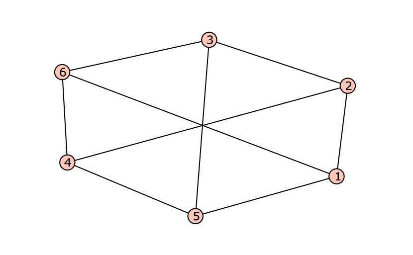
Figure 2. $S^{2}_{2}S^{2}_{1}K_{2}$

The next lemma informs us that, if we start with a matroid complex, this construction will usually result in another matroid. In fact, we will later, in Theorem 2.8, see that all matroids can be obtained from smaller matroids in this way. However, not every complex obtained by taking partial stars is matroid, even if we start with a “nice” complex (for example, paths can be obtained in this way). So, we must impose some additional conditions on this process. In particular, we need to choose the vertex we avoid properly, where the meaning of “properly” is given by the next definition.

Definition 2.6.

Let $\Delta$ be a simplicial complex and $v$ a vertex of $\Delta$. Then we say that $v$ is a center of $\Delta$ if $\operatorname{link}_{\Delta}(v)$ contains every other vertex of $\Delta$.

Note that this definition depends only on the 1-skeleton of $\Delta$; we are simply looking for vertices that are connected by an edge to every other vertex. More algebraically, if $I_{\Delta}$ is the Stanley-Reisner ideal of $\Delta$, $v$ is a center of $\Delta$ if and only if $x_{v}$ does not appear in any degree 2 minimal generator of $I_{\Delta}$.

In Figure 2 vertex 2 and 3 are the only centers, while Figure 2 shows us a complex that has no centers. If $\Delta$ is a cone then the apex of the cone is a center. The converse is false; to have a center it is only necessary that $\left[\Delta\right]_{1}$ be the 1-skeleton of a cone. This can be easily seen by looking at the Stanley-Reisner ideal and using the comment in the preceeding paragraph.

Lemma 2.7.

Let $\Delta$ be a matroid complex and $W=\{w_{1},\dotsc,w_{k}\}$ a set of vertices not in $\Delta$. Then $S_{v}^{W}\Delta$ is matroid if and only if $v$ is a center of $\Delta$.

Proof.

Assume that $v$ shares an edge with every other vertex of $\Delta$ (i.e., $v$ is a center of $\Delta$). Let $\Gamma=S_{v}^{W}\Delta$. If $X$ is a subset of vertices of $\Gamma$ which contains only vertices of $\Delta$ then ${\Gamma}|_{X}={\Delta}|_{X}$, which is pure. So suppose that $W\cap X\neq\emptyset$. If $v$ is the only vertex of $\Delta$ contained in $X$ then ${\Gamma}|_{X}$ is 0 dimensional and thus pure. So, assume that $X$ intersects the other vertices of $\Delta$. Let $X^{\prime}=X\cap[\operatorname{link}_{\Delta}(v)]_{0}$. Since $\Delta$ is matroid, ${\Gamma}|_{X^{\prime}}={\Delta}|_{X^{\prime}}$ is pure. A facet of ${\Gamma}|_{X}$ is of the form $\{v\}\cup E$ or $\{w_{i}\}\cup E$ where $E$ is a facet of ${\Gamma}|_{X^{\prime}}$. Since these all have the same size, ${\Gamma}|_{X}$ is pure and thus $\Gamma$ is matroid.

Now, suppose that $v$ is not a center and let $a\neq v$ be a vertex of $\Delta$ not in $\operatorname{link}_{\Delta}(v)$. If $\Delta$ is not pure then neither is $\Gamma=S_{v}^{W}\Delta$, so we may as well assume that $\Delta$ is pure. If $\Delta$ has dimension 0 then $v$ will be a facet of $\Gamma=S_{v}\Delta$, which will have dimension 1. Suppose that $\dim\Delta>1$. Then $\Delta_{\{a,v\}\cup W}$ has dimension 1 and has $\{v\}$ as a facet, thus is not pure so $\Gamma$ is not matroid. ∎

The next Theorem allows us to, in many cases, reduce large matroid complexes to much smaller ones. This is particularly useful if in dimension 1 where it gives a constructive procedure that produces all matroid complexes.

Theorem 2.8.

Let $\Delta$ be a simplicial complex with dimension $d$. Then $\Delta$ is matroid if and only if $\Delta=S_{v_{k}}^{m_{k}}\dotsm S_{v_{1}}^{m_{1}}\Gamma$ where $\Gamma$ is a matroid such that $\left[\Gamma\right]_{1}$ is a complete graph and the $v_{i}$ are distinct vertices of $\Gamma$. We allow for $\left[\Gamma\right]_{1}$ to be $K_{1}$, the complete graph on 1 vertex, i.e. a point.

To prove this, we must first establish the special case when $\dim\Delta=1$. Then, since the skeletons of matroids are themselves matroid, we can induct on the dimension and concern ourselves only with the facets of $\Delta$. That $\Delta$ has facets in the correct places will be forced by purity. The next lemma is used to easily detect the matroid-ness of a 1-dimensional complex. This result amounts to saying that we can walk between any 2 vertices of a 1-dimensional matroid complex by taking at most 2 steps (assuming our steps are 1 edge long).

Lemma 2.9.

Let $\Delta$ be a 1-dimensional simplicial complex. Then $\Delta$ is matroid if and only if for every vertex $v$ and every edge $E$, $\operatorname{link}_{\Delta}(v)\cap E\neq\emptyset$.

Proof.

Suppose there exists a vertex $v$ and an edge $E$ disjoint from the link of $v$. Let $L=[n]-\operatorname{link}_{\Delta}(v)$. Then $\Delta_{L}$ has $\{v\}$ and $E$ as facets, and so is not matroid.

Conversely, suppose that there exists a subset $W\subseteq[n]$ such that $\Delta_{W}$ is not pure. So $\Delta_{W}$ must have a 0-dimensional facet, say $\{v\}$. Let $v\neq w\in W$. Since $v$ is a facet of $\Delta_{W}$ we must have $\{v,w\}\not\in\Delta$. Thus $W\cap\operatorname{link}_{W}(v)=\emptyset$ and so any edge, $E$, of $\Delta_{W}$ (there must be at least one since $\Delta_{W}$ is not pure) must also be disjoint from $\operatorname{link}_{\Delta}(v)$. Since $E$ is also an edge of $\Delta$ the proof is complete. ∎

Lemma 2.10.

Let $\Delta$ be a matroid with dimension 1. Then $\Delta=S_{v_{k}}^{m_{k}}\dotsm S_{v_{1}}^{m_{1}}K_{s}$ where $k\leq s$ and the $v_{i}$ are distinct vertices of $K_{s}$.

Proof.

Let $v$ be a vertex of $\Delta$ and $n=f_{0}(\Delta)$. We define $\deg v=\deg_{\Delta}v=\lvert\operatorname{link}_{\Delta}(v)\rvert$. Choose, if possible, $v$ so that $\deg v\neq n-1$. If there are no such vertices then $\Delta=K_{n}$ and we are done. Let $W$ be the set of vertices of $\Delta_{-v}$ not in $\operatorname{link}_{\Delta}(v)$. If $E\in\Delta_{W}$ is an edge then $E\cap\operatorname{link}_{\Delta}(v)=\emptyset$, contradicting Lemma 2.9. So $\dim\Delta_{W}=0$. If $w\in W$ and $\{v,w\}\in\Delta$ then $w\in\operatorname{link}_{\Delta}(v)$, a contradiction. Let $\Delta^{\prime}$ be $\Delta$ with the vertices in $W$ deleted. From above, we can see that any edge of $\Delta$ that is not in $\Delta^{\prime}$ must be of the form $\{w,x\}$ where $w\in W$ and $x\in\operatorname{link}_{\Delta}(v)$. Thus, $\Delta=S_{v}^{m}\Delta^{\prime}$ where $m=\lvert W\rvert$. Since $\Delta^{\prime}$ has fewer vertices than $\Delta$ we can conclude by induction on $n$. ∎

Since any simplicial complex of the form $S_{v_{k}}^{m_{k}}\dotsm S_{v_{1}}^{m_{1}}K_{s}$ is matroid by Lemma 2.7, we now have a complete classification of 1 dimensional matroid complexes. Using this, we can now prove Theorem 2.8.

Proof.

Assume that $\Delta$ is matroid. We induct on $d$, the dimension of $\Delta$. If $d=0$ then $\Delta=S_{v}^{n-1}K_{1}$, where $v$ is the solitary vertex of $K_{1}$. So assume $d>0$ and choose $v\in\Delta$ to be a vertex such that $\operatorname{link}_{\Delta}(v)$ does not contain every other vertex of $\Delta$. If there are no such vertices then we may set $\Delta=\Gamma$ since the 1-skeleton of $\Delta$ must be complete. Let $W$ be the set of vertices not in $\operatorname{link}_{\Delta}(v)$. Let $\Delta^{\prime}$ be $\Delta$ with the vertices of $W$ deleted. We need only show that $\Delta=S_{v}^{W}\Delta^{\prime}$ since, by induction on the number of vertices, $\Delta^{\prime}$ has the required form. By Lemma 2.10 we have $[\Delta]_{1}=S_{v}^{W}[\Delta^{\prime}]_{1}$. In particular $[\Delta_{W}]_{1}$ has dimension 0. By definition, there are no edges (and thus no higher dimensional faces) of $\Delta$ in $\{v\}\cup W$. So, the only thing remaining to show is that, if $E$ is a facet of $\operatorname{link}_{\Delta}(v)$ (which is matroid and thus pure) and $w\in W$ then $\{w\}\cup E\in\Delta$. By induction on $d$, if $F\in\operatorname{link}_{\Delta}(v)$ is not a facet, $\{w\}\cup F\in W$. Suppose that $E\cup\{w\}\not\in\Delta$. Let $X=\{v,w\}\cup E$. For every $e\in E$, $(E-\{e\})\cup\{w\}\in\Delta_{X}$ and since $E\cup\{w\}\not\in\Delta_{X}$ these are all facets. By construction, $E\cup\{v\}\in\Delta_{X}$ contradicting the purity of $\Delta_{X}$. Thus, $E\cup\{w\}\in\Delta$. Finally, we note that if $E\cup\{w\}\in W$ where $w\in W$ and $E\not\in\operatorname{link}_{\Delta}(v)$ then an identical argument (interchanging $v$ and $w$) shows that, again, $\Delta_{\{v,w\}\cup E}$ is not pure. Therefore, $\Delta=S_{v}^{W}\Delta^{\prime}$ and we may conclude by induction on the number of vertices.

For the converse we simply note that, by Lemma 2.7, every complex of the form $S_{v_{k}}^{m_{k}}\dotsm S_{v_{1}}^{m_{1}}\Gamma$ is matroid by provided that we choose the $v_{i}$ so that they are centers of their respective complexes. Being a center depends only the 1-skeleton, which is, by assumption, complete. So we can simply choose the $v_{i}$ to be distinct vertices of $\Gamma$ and be assured that the partial star avoiding $v_{i}$ is matroid. ∎

3. Dimension 1

Our goal is to classify the h-vectors of all 1-dimensional matroid complexes. In fact, we do something stronger and classify all 1-dimensional matroid complexes up to isomorphism in terms of partitions.

Since we will be working exclusively with 1-dimensional complexes, it will be convenient to ignore the difference between the 0-dimensional complex $\operatorname{link}_{\Delta}(k)$ and the set of vertices of $\operatorname{link}_{\Delta}(k)$.

Lemma 2.10 provides us with a complete classification of 1 dimensional matroid complexes. It only remains to compute the possible $h$-vectors that this construction allows. Note that Lemma 2.7 allows us to form a new matroid complex $S^{1}_{v}\Delta$ whenever $\Delta$ has a center. If $\Delta$ has no center then we can easily give it a center by using the next lemma.

Lemma 3.1.

Let $\Delta$ be a 1-dimensional matroid complex with h-vector $(1,m-1,h_{2})$ and $C_{1}\Delta$ the 1-skeleton of the cone over $\Delta$. Then $C_{1}\Delta$ is matroid with h-vector $(1,m,h_{2}+m)$.

Proof.

Proposition 2.3 shows that the cone of $\Delta$ and its 1-skeleton, $C_{1}\Delta$ are matroid. The statement about h-vectors follows by noting that the f-vector of $C_{1}\Delta$ is $(1,m+2,f_{2}+m+1)$ where $f_{2}$ is the number of edges of $\Delta$. ∎

While the title says “$h$-vector”, we mostly work by computing $f$-vectors. It will thus be convenient to use Equation (1) to write the $h$-vector of a complex with $f$-vector $(1,f_{0},f_{1})$ as

$$h=(1,f_{1}-2,1-f_{1}+f_{2}).$$

So, if $\Delta$ has $h$-vector $(1,m,h_{2})$ then $S_{v}^{i}\Delta$ will have $h$-vector $(1,m+i,h_{2}+mi)$ since we are adding in exactly $mi$ additional edges and $i$ vertices. If we wish to stay in the class of matroid complexes then we must require that $\Delta$ have a center. If it doesn’t then we first apply $C_{1}$. These two constructions in fact give every 1-dimensional matroid complex on $n$ vertices and gives us a way to compute the $h$-vector. Here the degree of a vertex $v$ is the number of edges containing $v$. Note that $v$ is a center of $\Delta$ if and only if $v$ has degree $n-1$.

Theorem 3.2.

Let $h=(1,m,h_{2})$. Then $h$ is the $h$-vector of a 1-dimensional matroid complex if and only if one of the following holds.

1. $h_{2}=x(m-x)$ for some $\lfloor\frac{m}{2}\rfloor\leq x\leq m$.

2. $h_{2}=h^{\prime}+x(m-x+1)$ where $\lfloor\frac{m}{2}\rfloor\leq x\leq m$ and $(1,x-1,h^{\prime})$ is the h-vector of a matroid complex.

Proof.

Suppose that $\Delta$ is a matroid complex with $h$-vector $h$. Let $v$ be a vertex of $\Delta$ with degree $x+1$ and $L=\operatorname{link}_{\Delta}(v)\cup\{v\}$. If $x=m=n-2$ and $\Delta$ is not a cone then we may delete $v$ to obtain a matroid complex $\Delta_{-v}$ with h-vector $(1,m-1,h^{\prime})$. So the h-vector of $\Delta$ is $(1,m,h^{\prime}+m)$, which satisfies condition 2 with $x=m$. If $\Delta$ is a cone then it satisfies condition 1 with $x=m$.

Assume $x\neq m$ and let $\Gamma={\Delta}|_{L}$ If $w\in L-\{v\}$ and $a\not\in L$ then $\{a,w\}\in\Delta$ by Lemma 2.9. So we may write $\Delta=S_{v}^{[n]-L}\Gamma$. By definition $\lvert L\rvert=x+2$ and $h(\Gamma_{-v})=(1,x-1,h^{\prime})$ for some $h^{\prime}$, as long as $\dim\Gamma_{-v}=1$ (equivalently, as long as $\Gamma$ is not a cone). Now simply note that $\lvert[n]-L\rvert=n-x-2=m-x$ and that to form $\Delta$ from $\Gamma_{-v}$ we must add edges $\{a,b\}$ for every $a\in L-\{v\}$ and $b\not\in L-\{v\}$. There are a total of $x(m-x+1)$ such edges. Thus $h_{2}(\Delta)=h^{\prime}+x(m-x+1)$. Now suppose that $\Gamma$ is a cone so that $h(\Gamma)=(1,x,0)$. Then from the comment just before the proof, we see that the $h$-vector of $\Delta$ is given by $(1,m,h_{2})$ where $h_{2}=0+x\lvert[n]-L\rvert=x(m-x)$.

To get the inequalities, we simply take $v$ to be a vertex with maximal degree. If $x<\lfloor\tfrac{m}{2}\rfloor$ then each vertex, $w\in L$, of $\Delta=S^{[n]-L}_{v}\Gamma$ has every vertex not in $L$ in its link, by construction. There are $m-x\geq\lfloor\tfrac{m}{2}\rfloor$ such vertices meaning that $w$ has a larger degree than $v$.

Conversely, if $h$ satisfies one of the 2 conditions above, we must show that there is some matroid with $h$-vector $h$. There are naturally 2 cases.

1. If $h=x(m-x)$ then the preceding paragraph tells us how to construct the matroid $\Delta$. Let $\Gamma$ be the cone over $x-1$ vertices with apex $v$ and $\Delta=S^{m-x}_{v}\Gamma$. As noted above, $h(\Delta)=(1,m,x(m-x))$.

2. Suppose $h=h^{\prime}+x(m-x+1)$ and there is some matroid, $\Gamma$ with $h$-vector $(1,x-1,h^{\prime})$. Again, the needed construction is implicit in the preceding argument. We have that $C_{1}\Gamma$ is matroid with $h$-vector $(1,x,h^{\prime}+x)$ and $\Delta=S_{v}^{m-x}C_{1}\Gamma$ has $x+1+1+(m-x)=m+2$ vertices and $h_{2}(\Delta)=h^{\prime}+x+x(m-x)=h^{\prime}+x(m-x+1)$. We choose the vertex $v$ to be the new vertex added when forming $C_{1}\Gamma$ so that we may be assured that it is a center and that $\Delta$ is matroid (by Lemma 2.7).

∎

Shortly, we will give a more closed form of the same classification (Theorem 3.5) that proves to be easier to work with in many cases. However, in some specific cases it is computationally easier to use Theorem 3.2 to check that a given sequence is a matroid $h$-vector (or not) than to use Theorem 3.5.

Remark 3.3.

Using the above theorem, we can produce several easy examples of matroid $h$-vectors (assuming in each case that the final entry is positive): $(1,m,m)$, $(1,m,m-1)$, $(1,m,2(m-1))$, $(1,m,2(m-2))$, $(1,m,3m-5)$. The last is produced using $x=m-1$ and $h^{\prime}=m-3$, if $m\geq 3$ since $(1,m-2,m-3)$ is a matroid $h$-vector.

Remark 3.4.

Theorem 3.2 provides us with a method for checking whether or not there is a matroid with the specified $h$-vector. In specific cases this can be somewhat tedious (although it is easily automated) however, we can eliminate certain small values immediately.

1. There are no matroid $h$-vectors of the form $(1,m,h_{2})$ where $0<h_{2}<m-1$ because if there were then we would also have a matroid $h$-vector of the form $(1,x-1,x(m-x+1))$ for some $x$. However $x(m-x+1)>x(m-x)\geq m-1$ for all $1\leq x<m$ (which excludes the first type of $h$-vectors as well).

2. Suppose $m\geq 6$ and $m<h_{2}<2(m-2)$. Then $(1,m,h_{2})$ is not the $h$-vector of a matroid complex. To see this, note that the function $g(x)=x(m-x)$ only takes on values larger than $2(m-2)$ when $1<x<m-1$ and $g(1)=g(m-1)=m-1$, excluding $h$-vectors of the first type. Similarly, the function $f(x)=x(m-x+1)$ takes on only values larger than $2(m-2)$ except for $f(1)=f(m)=m$. Thus, if $(1,m,h_{2})$ is a matroid $h$-vector then there must be another matroid $h$-vector $(1,m-1,h_{2}-m)$. But $0<h_{2}-m<(m-1)-1$ and so by the above, there are no such $h$-vectors.

We now give a more closed form of Theorem 3.2. If $\Delta$ is a 1-dimensional matroid then, by Lemma 2.10 we know that we may write $\Delta$ in the form

$$\Delta=S_{v_{1}}^{W_{1}}\dotsm S_{v_{k}}^{W_{k}}K_{s}.$$

From this it is straightforward to compute the $f$-vector and $h$-vector of $\Delta$.

Theorem 3.5.

Let $h=(1,n-2,h_{2})$, $h_{2}\geq 0$. Then $h$ is the $h$-vector of a matroid if and only if there is a sequence of numbers $m_{1},m_{2},\dotsc,m_{k}$ such that $m_{1}\geq 0$, $\sum_{i=1}^{k}m_{i}=n-k$ and

$$h_{2}=\binom{n-1}{2}-\sum_{i=1}^{k}\binom{m_{i}+1}{2}$$

Proof.

Assume $h$ is the $h$-vector of some matroid, $\Delta$. If $\Delta$ is not the complete graph on $n$ vertices, $K_{n}$ (for which the claim is obvious) then, we may write $\Delta=S_{v_{1}}^{W_{1}}\dotsm S_{v_{k}}^{W_{k}}K_{s}$. Let $m_{i}=\lvert W_{i}\rvert$. By construction, $\dim\Delta_{W_{i}\cup\{v_{i}\}}=0$ and, if $X$ is not contained in any $W_{i}$, $\dim\Delta_{X}=1$. Moreover, all of the $W_{i}\cup\{v_{i}\}$ are pairwise disjoint. Our construction guarantees that, if $E$ is an edge not contained in any $W_{i}\cup\{v_{i}\}$ then $E\in\Delta$. It follows that $f_{1}(\Delta)=\binom{n}{2}-\sum\binom{m_{i}+1}{2}$. It is now easy to compute the $h$-vector of $\Delta$ and see that it is as claimed.

Conversely, if $h$ has the form given in the Theorem, we may set $\Delta=S_{v_{1}}^{m_{1}}\dotsm S_{v_{k}}^{m_{k}}K_{s}$, which, as we see above, is matroid and has the correct $h$-vector.

∎

If $m\in\mathbb{N}^{s}_{0}$ and $\Delta=S^{m_{s}}_{v_{s}}\dotsm S^{m_{1}}_{v_{1}}K_{s}$, where the $v_{i}$ are distinct vertices of $K_{s}$ then it is easily seen that if we choose the $v_{i}$ in a different order we get isomorphic complexes (see Lemma 3.10). So without loss of generality, we will always assume that $v_{i}=i$ and suppress the notation.

Definition 3.6.

If $m\in\mathbb{N}_{0}^{s}$ then we define $\Delta_{\mathbf{m}}=S^{m_{s}}\dotsm S^{m_{1}}K_{s}$ where we agree that if $m_{i}=0$ then $S^{m_{i}}\Gamma=\Gamma$ for any complex $\Gamma$.

Remark 3.7.

So, what we have (from Lemma 2.10) is that every 1-dimensional matroid is isomorphic to one of the form $\Delta_{\mathbf{m}}$ for some sequence, $\mathbf{m}$, of non-negative integers with length $s$. However, we have chosen to construct $\Delta_{\mathbf{m}}$ in such a way that the first $s$ vertices form a complete graph. Of course, we may always permute the vertices so that this occurs. The point is that, while Lemma 2.10 completely classifies all matroids with dimension 1, the notation $\Delta_{\mathbf{m}}$ does not since it implicitly assumes a particular ordering of the vertices. Since the author does not distinguish between isomorphic complexes, this may be considered only a minor notational annoyance.

If $\mathbf{m}=\mathbf{0}$ is the zero sequence then $\Delta_{\mathbf{0}}=K_{s}$ and if $\mathbf{m}=(m_{1})$ then (with the understanding that $K_{1}$ is a single vertex) $\Delta_{(m_{1})}$ is a 0-dimensional complex with $m_{1}+1$ vertices. Of course, all 0-dimensional complexes are matroid. In all other cases, $\dim\Delta_{\mathbf{m}}=1$ as noted below in Proposition 3.20 (a).

The following is a restatement of Theorem 3.5 using this new notation.

Corollary 3.8.

If $m\in\mathbb{N}_{0}^{s}$ then $h$-vector of $\Delta_{\mathbf{m}}$ is $(1,h_{1},h_{2})$ where

$$h_{1} =s+\sum_{i=1}^{s}m_{i}$$

$$h_{2} =\binom{n-1}{2}-\sum_{i=1}^{s}\binom{m_{i}+1}{2}$$

Using an argument similar to that of Theorem 3.5 we can describe algebraically the structure of all possible Stanley-Reisner ideals of 1 dimensional matroid complexes.

Notation.

If $\sigma\subseteq[n]$ then $\mathfrak{m}_{\sigma}=\left\langle x_{i}\mid i\in\sigma\right\rangle$ (we will write $\mathfrak{m}=\mathfrak{m}_{[n]}$) and $\hat{\mathfrak{m}}_{\sigma}^{d}$ is the ideal generated by all the squarefree monomials in $\mathfrak{m}^{d}$. If $\lvert\sigma\rvert<d$ then $\hat{\mathfrak{m}}_{\sigma}^{d}=\left\langle 0\right\rangle$.

Theorem 3.9.

Let $I\subseteq S$. Then $I$ is the Stanley-Reisner ideal of a 1-dimensional matroid on $[n]$ with $n$ vertices if and only if $I$ has the form

(2) $$I=\sum_{i=1}^{k}\hat{\mathfrak{m}}_{\sigma_{i}}^{2}+\hat{\mathfrak{m}}^{3}$$

for some collection $\{\sigma_{i}\}$ of subsets of $[n]$ such that $\sigma_{i}\cap\sigma_{j}=\emptyset$ whenever $i\neq j$ and $n\geq\sum_{i=1}^{k}\lvert\sigma_{i}\rvert$.

Proof.

Assume $I=I_{\Delta}$ for some 1-dimensional matroid $\Delta$ on $[n]$. Then we may write $\Delta=\Delta_{\mathbf{m}}=S^{W_{k}}_{v_{k}}\dotsm S^{W_{1}}_{v_{1}}K_{s}$, where $\lvert W_{i}\rvert=m_{i}$. We consider $\mathbf{m}\in\mathbb{N}^{s}$, padding the end with 0 if needed. Then the number of vertices of $\Delta$ is $s+\sum m_{i}=n$. Let $\sigma_{i}\mathrel{\mathop{:}}=W_{i}\cup\{v_{i}\}$. The $\sigma_{i}$ are all pairwise disjoint and $\lvert\sigma_{i}\rvert=m_{i}+1$ We then get that $n=\sum_{i=1}^{k}\lvert\sigma_{i}\rvert+(s-k)$, where $s-k\geq 0$. By construction, any edge in $\sigma_{i}$ is a non-face of $\Delta$ and thus any squarefree monomial in $\hat{\mathfrak{m}}^{d}_{\sigma_{i}}$ is in $I$. Again the construction assures us that these are the only non-edges of $\Delta$. Since $\dim\Delta=1$ every degree 3 squarefree monomial must also be in $I$. Thus $I$ has the form given in equation (2).

Conversely, assume $I$ is of the form given in equation (2). Then set $m_{i}=\lvert\sigma_{i}\rvert-1$ and $s=n-\sum m_{i}$. Let $m=(m_{1},\dots,m_{k},0,\dotsc,0)\in\mathbb{N}^{s}$. The argument above shows us that $I$ is the Stanley-Reisner ideal of $\Delta_{\mathbf{m}}$. ∎

Using our knowledge of the Stanley-Reisner ideal, we show that $\Delta_{\mathbf{m}}$ is invariant up to isomorphism when the entries of $\mathbf{m}$ are permuted.

Lemma 3.10.

Let $\tau$ be a permutation on $[s]$ and $\tau\mathbf{m}=(m_{\tau 1},\dotsc,m_{\tau s})$. Then $\Delta_{\mathbf{m}}\cong\Delta_{\tau\mathbf{m}}$

Proof.

Let $I$ and $J$ be the Stanley-Reisner ideals of $\Delta_{\mathbf{m}}$ and $\Delta_{\tau\mathbf{m}}$ respectively. Write

$$I=\sum_{i=1}^{k}\hat{\mathfrak{m}}_{\sigma_{i}}^{2}+\hat{\mathfrak{m}}^{3}$$

and

$$J=\sum_{i=1}^{k}\hat{\mathfrak{m}}_{\eta_{i}}^{2}+\hat{\mathfrak{m}}^{3}.$$

Clearly, $\lvert\sigma_{\tau i}\rvert=\lvert\eta_{i}\rvert$ and so since they are all pairwise disjoint, $\lvert\cup\sigma_{i}\rvert=\lvert\cup\eta_{i}\rvert$. We may as well assume that they are equal to each other and equal to $[r]$ for some $r\leq n$. Select a bijection $\phi_{i}\colon\sigma_{\tau i}\to\eta_{i}$ for each $i$. Pasting these together (which is well defined only because the $\sigma_{i}$ and $\eta_{j}$ are pairwise disjoint) gives a permutation on $[n]$ (fixing everything not in $[r]$). This now induces an isomorphism $I\cong J$ which implies that $\Delta_{\mathbf{m}}$ and $\Delta_{\tau m}$ are isomorphic as well. ∎

Remark 3.11.

While the sequence $\mathbf{m}$, up to permutation, does uniquely determine the isomorphism class of the complex $\Delta_{\mathbf{m}}$, the $h$-vector does not. The matroids $\Delta_{(2,2)}$ and $\Delta_{(3,0,0)}$ both have $h$-vector $(1,4,4)$ but are not isomorphic since $\Delta_{(3,0,0)}$ has a vertex with degree 5 but all the vertices of $\Delta_{(2,2)}$ have degree 3. These complexes are depicted in Figures 2 and 2.

Similarly, the isomorphism class of a 1-dimensional matroid, $\Delta$, is determined by the degree sequence of $\Delta$. If $\Delta$ is a 1-dimensional complex (which we may regard as a graph) and $v$ is a vertex of $\Delta$ the we define the degree of $v$, $\deg v=\deg_{\Delta}v$ to be the number of edges containing $v$, or equivalently, the number of vertices in its link. The degree sequence of $\Delta$, $D(\Delta)$, is a sequence defined by $D_{i}=\lvert\{v\in\Delta\mid\deg v=i\}\rvert$.

Lemma 3.12.

If $\Delta$ and $\Delta^{\prime}$ are 1-dimensional matroids on $[n]$ then $\Delta\cong\Delta^{\prime}$ if and only if $D(\Delta)=D(\Delta^{\prime})$.

Proof.

It is trivial that isomorphic complexes have equal degree sequences, so we only consider the other direction. Since the degree sequence determines $f_{0}(\Delta)$, we may assume that $f_{0}(\Delta)=f_{0}(\Delta^{\prime})=n$. Let $v$ be a vertex of $\Delta$ with minimal degree. If $\deg v=n-1$ then $\Delta=K_{n}$. But this is the only complex with degree sequence $D(K_{n})$ ($D_{n-1}(K_{n})=n$ and all other are 0). So assume that $\deg v<n-1$. Let $v^{\prime}$ be a vertex of $\Delta^{\prime}$ with $\deg v=\deg v^{\prime}$. Without loss of generality, we may write $\Delta=\Delta_{\mathbf{m}}$.

Since $\Delta_{\mathbf{m}}$ is invariant under permutations of the entries of $\mathbf{m}$ we may, still without loss of generality, assume that $v$ is in the last group of vertices to be added and likewise for $v^{\prime}$ or they are the vertices being avoided. Then $\Delta_{-v}$ and $\Delta^{\prime}_{-v^{\prime}}$ have the same degree sequence (the degree of each vertex in the link of $v$ ($v^{\prime}$) goes down by 1 and the others stay fixed). So, by induction on the number of vertices there is an isomorphism $\Delta_{-v}\to\Delta^{\prime}_{-v^{\prime}}$. since $v$ and $v^{\prime}$ must both be “attached” to their deletions in the same manner (by the construction of $\Delta_{\mathbf{m}}$) this will lift to an isomorphism simply by mapping $v\mapsto v^{\prime}$. ∎

Remark 3.13.

Since we can permute the entries of $\mathbf{m}$ as we like, we may as well assume that $m_{1}\geq m_{2}\geq\dotsm\geq m_{s}$. Let $k=\max\{i\mid m_{i}\neq 0\}$. If $\Delta_{\mathbf{m}}$ has $n$ vertices then $n=s+\sum_{i=1}^{s}m_{i}=s+\sum_{i=1}^{k}m_{i}$ or equivalently, $(m_{1},\dotsc,m_{k})$ is a partition of $n-s$ with length $k\leq s$. By increasing each entry by 1, we can form a partition $\lambda=(m_{1}+1)+\dotsm+(m_{s}+1)$ of $n$. Thus, each 1 dimensional matroid complex corresponds to a partition, $\lambda$, of $n$ and two matroids are isomorphic if and only if they have the same partition.

The partition, $\lambda$, is determined uniquely by the non-zero entries of $\mathbf{m}$ and $n$. It is often notationally more convenient to specify $\mathbf{m}$ instead of $\lambda$ as $n$ is usually understood.

Example 3.14.

Let $n=6$. Then, as in the above remark, the partitions we are concerned with are summarized in the following table (we allow $\emptyset$ as the unique partition of 0).

$n-s$	$s$	partitions	$m$
		of $n-s$
0	6	$\emptyset$	000000
1	5	1	10000
2	4	11	1100
		2	2000
		111	111
3	3	21	210
		3	300
		31	31
4	2	22	22
		4	40
5	1	5	5

The last is the 0-dimensional matroid with 6 vertices. This means we have a total of 10 matroids on 6 vertices (see Table 1). But there are only 8 distinct $h$-vectors of such complexes (those that end with 10, 9, 8, 7, 6, 4, 3 and 0), such there must be either 2 $h$-vectors each with 2 matroids or a single $h$-vector with 3 matroids. The matroids $\Delta_{22}$ and $\Delta_{300}$ both have $h$-vector $(1,4,4)$ and $\Delta_{2000}$ and $\Delta_{111}$ both have $h$-vector $(1,4,7)$. See Figure 3.

A similar computation with $n=7$ shows that there are a total of 14 1-dimensional matroids with 7 vertices but only 12 matroid $h$-vectors. As with $n=6$ there are two pairs of non-isomorphism matroids with the same $h$-vector. In this case it is $\Delta_{3000}$ and $\Delta_{2200}$ sharing the $h$-vector $(1,5,9)$ along with $\Delta_{1110}$ and $\Delta_{20000}$ having $h$-vector $(1,5,12)$.

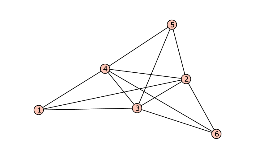
Figure 3. $\Delta_{111}$ and $\Delta_{2000}$ have the same $h$-vector but are not isomorphic

Remark 3.15.

As we see in the above example a partition of $n$ does not necessarily produce of 1 dimensional complex. However the only exception is the trivial partition $\lambda=n$, which is the complex of $n$ vertices. We can see from the definition of $\Delta_{\mathbf{m}}$ that as long as the length of $\mathbf{m}$ is at least 2, $\Delta_{\mathbf{m}}$ will contain a complete graph on at least 2 vertices and so $\dim\Delta_{\mathbf{m}}=1$.

Notation.

If $\lambda$ is a partition of $n$ then we will write $\lvert\lambda\rvert=n$ and $\ell(\lambda)$ for the length of $\lambda$. If $k>1$ then $\lvert\lambda\rvert_{k}=\sum\binom{\lambda_{i}}{k}$ where we adopt the convention that $\binom{a}{b}=0$ if $a<b$.

Definition 3.16.

1. If $\lambda$ is a partition of $n$ then $\Delta_{\lambda}$ is the isomorphism class of the matroid defined by the sequence $(\lambda_{1}-1,\dotsc,\lambda_{\ell(\lambda)}-1)$; $h(\lambda)$ is their common $h$-vector.

2. If $\Delta\cong\Delta_{\mathbf{m}}$ is a matroid then $\lambda_{\Delta}$ is the partition $\sum_{i=1}^{s}(m_{i}+1)$ of $n$. We will call $\lambda_{\Delta}$ the partition associated to $\Delta$.

We have defined $\Delta_{\lambda}$ so that it is not a simplicial complex itself, but is rather a set of isomorphic simplicial complexes. We will, nonetheless, continue to write things like $\dim\Delta_{\lambda}$ and $h(\Delta_{\lambda})$ to refer to any invariant of the class. We will also misuse such notation as $C\Delta_{\lambda}$ to refer to the class of complexes obtained from $\Delta_{\lambda}$ by, in this example, taking the cone.

Example 3.17.

Consider again Figure 3, which depicts the matroids corresponding to the sequences $(1,1,1)$ and $(2,0,0,0)$ respectively. These are elements of the classes $\Delta_{2+2+2}$ and $\Delta_{3+1+1+1}$. Permuting the entries of the sequences will permute the vertices of the complexes. This will leave $\Delta_{111}$ unchanged. But, we can relabel the vertices so that $\{1,2,3\}$ does not defined a complete graph, which cannot be obtained by permuting the entries of $(1,1,1)$. This is an element of $\Delta_{2+2+2}$ that is not of the form $\Delta_{\mathbf{m}}$ for any sequence $\mathbf{m}$, which does not prevent it from being matroid.

Theorem 3.18.

There is a bijection between isomorphism classes of matroid complexes with dimension at most 1 and $n$ vertices and partitions of $n$. In particular the number of isomorphism classes of 1 dimensional matroids with $n$ vertices is $p(n)-1$ where $p(n)$ is the number of partitions of $n$.

Proof.

The bijection is $\lambda\mapsto\Delta_{\lambda}$. The map $\Delta\mapsto\lambda_{\Delta}$ is its inverse. That every matroid with dimension 1 can be written as $\Delta_{\lambda}$ is essentially the content of Lemma 2.10. Proposition 3.20(a) takes care of the case when $\dim\Delta=0$. That these maps are inverses to each other follows from their definitions. ∎

Remark 3.19.

If $\lambda\neq n$ is a partition then $h(\lambda)=(1,n-2,h_{2})$ where $n=\lvert\lambda\rvert$ and

$$\begin{split}h_{2}(\Delta_{\lambda})&=\binom{n-1}{2}-\sum_{i=1}^{\ell(\lambda)}\binom{\lambda_{i}}{2}\\ &=\binom{n-1}{2}-\lvert\lambda\rvert_{2}.\end{split}$$

So two partitions, $\lambda$ and $\lambda^{\prime}$ determine the same $h$-vector if and only if $\lvert\lambda\rvert=\lvert\lambda^{\prime}\rvert$ and $\lvert\lambda\rvert_{2}=\lvert\lambda\rvert_{2}$. Examples of such pairs can be seen in Example 3.14. The first such pairs are $\lambda=3+1+1$, $\lambda^{\prime}=2+2+2$ and $\lambda=3+3$, $\lambda^{\prime}=4+1+1$.

Suppose there are $k$ entries of $\lambda$ equal to 1 and $\lambda^{\prime}$ is the partition of $n-k$ with these entries removed. Then $\sum\binom{\lambda_{i}}{2}=\sum\binom{\lambda^{\prime}_{i}}{2}$. Then $\Delta_{\lambda}=C_{1}\dotsm C_{1}\Delta_{\lambda^{\prime}}$ (see the Proposition below) and $h(\lambda)$ is easily determined from $h(\lambda^{\prime})$. So, in this sense, every matroid $h$-vector is induced from the $h$-vector of a smaller complex, one whose associated partition has no entry equal to 1.

The next proposition collects various facts about the relationship between 1-dimensional matroids and their associated partitions. If $\lambda$ and $\lambda^{\prime}$ are partitions then we write $\lambda+\lambda^{\prime}$ for the concatenation of $\lambda$ and $\lambda^{\prime}$ as a partition of $\lvert\lambda\rvert+\lvert\lambda^{\prime}\rvert$. Likewise, $\mathbf{m},\mathbf{m^{\prime}}$ is the concatenation of the sequences $\mathbf{m}$ and $\mathbf{m^{\prime}}$.

Proposition 3.20.

1. $\dim\Delta_{\lambda}=0$ if and only if $\ell(\lambda)=1$.

2. $\Delta_{\mathbf{m},\mathbf{m^{\prime}}}\cong[\Delta_{\mathbf{m}}\ast\Delta_{\mathbf{m^{\prime}}}]_{1}$, the one-skeleton of the join. Likewise for $\Delta_{\lambda+\lambda^{\prime}}$.

3. $\Delta_{\mathbf{m},0}\cong C_{1}\Delta_{\mathbf{m}}$ or equivalently $\Delta_{\lambda+1}=C_{1}\Delta_{\lambda}$.

4. $\Delta_{\lambda}$ is a cone if and only if $\lambda=(n-1)+1$

5. If $\Delta$ and $\Delta^{\prime}$ are 1 dimensional matroids with $n$ vertices then $h(\Delta)=h(\Delta^{\prime})$ if and only if $\binom{n-1}{2}-h_{2}(\lambda_{\Delta})=\binom{n-1}{2}-h_{2}(\lambda_{\Delta^{\prime}})$.

6. (Klivans) A 1 dimensional matroid, $\Delta_{\mathbf{m}}$, is isomorphic to a shifted complex if and only if $\mathbf{m}$ contains at most 1 non-zero entry.

Proof.

1. This follows immediately from the definition of $\Delta_{\lambda}$, which is formed starting with a complete graph on $\ell(\lambda)$ vertices. Of course, this has dimension 0 if and only if $\ell(\lambda)=1$.

2. We induct on the length of $\mathbf{m^{\prime}}$. If $\mathbf{m}$ has length 1 then $\dim\Delta_{\mathbf{m}}=0$ and, by the definition $\Delta_{\mathbf{m}}\ast\Delta_{\mathbf{m^{\prime}}}=\Delta_{\mathbf{m},\mathbf{m^{\prime}}}$. Now, if $\mathbf{m^{\prime}}$ has length $s>1$ let $\mathbf{m^{\prime\prime}}=(m_{1},\dotsc,m_{s-1})$. Then

   $$\Delta_{\mathbf{m},\mathbf{m^{\prime}}}\cong\Delta_{\mathbf{m},\mathbf{m^{\prime\prime}},m_{s}} \cong[\Delta_{\mathbf{m},\mathbf{m^{\prime\prime}}}\ast\Delta_{m_{s}}]_{1}$$

   $$\cong[(\Delta_{\mathbf{m}}\ast\Delta_{\mathbf{m^{\prime\prime}}})\ast\Delta_{m_{s}}]_{1}$$

   $$\cong[\Delta_{\mathbf{m}}\ast\Delta_{\mathbf{m^{\prime}}}]_{1}$$

   since the join is associative.

3. $C_{1}\Delta$ is the 1-skeleton of $C\Delta$, the join of $\Delta$ and a single vertex. So this follows from part (b).

4. From part (a), $\Delta_{m_{1}}$ has dimension 0 and from part (c) $\Delta_{\mathbf{m}}=C_{1}\Delta_{m_{1}}=C\Delta_{m_{1}}$ Conversely, if the sequence $\mathbf{m}$ has more than 1 non-zero entry $\Delta_{\mathbf{m}}$ can not be a cone, since it can then be written as the 1-skeleton of the join of two smaller complexes, at least one of which is not a cone. So $\ell(\lambda_{\Delta})=1$ and $\Delta_{\mathbf{m}}=C_{1}\dotsm C_{1}\Delta_{m_{1}}$, which is not a cone if there is more than one $C_{1}$.

5. This follows immediately from Corollary 3.8 after noting that $\Delta_{\lambda}$ has $\lvert\lambda\rvert$ vertices.

6. Let $\lambda=\lambda_{\Delta}$. By Theorem 3.9, we can write

   $$I=\sum_{i=1}^{k}\hat{\mathfrak{m}}_{\sigma_{i}}^{2}+\hat{\mathfrak{m}}^{3}$$

   where $\lvert\sigma_{i}\rvert=\lambda_{i}$. We need to see that this ideal is squarefree strongly stable if and only if $\lambda_{i}=1$ for all $i>1$. One direction is easy; if only $lambda_{1}=1$ then it is clear that $I_{\Delta}$ will be squarefree strongly stable (after permuting the indices that so that $\sigma_{1}$ is the first $\lvert\sigma_{1}\rvert$ variables). Conversely, if $\lambda_{2}\neq 1$ and $x_{i}x_{j}$ is the product of the two variables with the smallest indices in $\sigma_{2}$, $x_{i-1}x_{j}\not\in I_{\Delta}$ since (by construction) $\{i-1,j\}\not\subseteq\sigma_{2}$ and it cannot be contained in any other $\sigma_{i}$ since they are all pairwise disjoint. Thus $I_{\Delta}$ is not squarefree strongly stable whenever $\ell(\lambda)>1$ (no matter how we permute the indices)

∎

Remark 3.21.

Part (f) of Proposition 3.20 is in fact the same statement as Proposition 1 of [9] which states that dimension 1 (or rank 2) shifted matroids are exactly those obtained by starting with a dimension 0 complex and applying the $C_{1}$ operator repeatedly. This means precisely that our matroid is isomorphism to one of the form the form $\Delta_{(m_{1},0,0,\dotsc,0)}$. Equivalently, $\Delta_{\lambda}$ contains a shifted complex if and only if $\lambda$ has only one entry not equal to 1.

If we regard the dimension 1 simplicial complex, $\Delta$, as a graph one might want to ask about the size of the maximal cliques (that is, maximal subsets of vertices, $W$ so that ${\Delta}|_{W}$ is a complete graph). If $\Delta$ is matroid then this is easy to determine from looking at the partition $\lambda_{\Delta}$.

Lemma 3.22.

If $\dim\Delta=1$ and $\Delta$ is matroid then, regarding $\Delta$ as a graph, all the maximal cliques of $\Delta$ have $\ell(\lambda_{\Delta})$ vertices.

Proof.

Let $\lambda=\lambda_{\Delta}$. Of course, the sizes of the maximal cliques depends only on the isomorphism type of $\Delta$, so we may assume that $\Delta=\Delta_{\mathbf{m}}$, where $m_{i}=\lambda_{i}-1$. Let $s=\ell(\lambda)$. By definition, ${\Delta}|_{[s]}$ is a complete graph.

We may assume that $\lambda$ is ordered so that $\lambda_{1}\geq\lambda_{2}\geq\dotsm$. If $\Delta$ is itself a complete graph, then it is it’s own unique maximal clique. This only happens if $\lambda=1+1+\dotsm+1$. Ignoring this single exception, we now assume that $\lambda_{1}>1$. Let $v$ be one of the $\lambda_{1}-1$ vertices of $\Delta_{\mathbf{m}}$ added in the first batch (those avoiding vertex 1). Then $\lambda_{\Delta_{-v}}=(\lambda_{1}-1)+\lambda_{2}+\dotsm+\lambda_{s}$. This partition also has length $s$ (since $\lambda_{1}>1$), so all its maximal cliques have size $s$, by induction on the number of vertices. If $W$ is a maximal clique of $\Delta$ then, if $v\not\in W$, $W$ is also a maximal clique of $\Delta_{-v}$ and therefore $\lvert W\rvert=s$. Suppose that $v\in W$. Then $W-\{v\}$ is certainly a clique of $\Delta_{-v}$, and we claim that it has size $s-1$.

To see this, we first claim that $W^{\prime}=(W-\{v\})\cup\{1\}$ is a maximal cliques and so has $s$ elements. Let $w\in W-\{v\}$ and suppose that $\{1,w\}\not\in\Delta_{-v}$. Since $W$ is a clique, $\{w,v\}\in\Delta$. Using Lemma 2.9, we see that $\operatorname{link}_{\Delta}(1)\cup\{w,v\}$ must be in $\Delta$. Since $\{1,w\}$ is not in $\Delta$ we must have $\{1,v\}\in\Delta$. But, by our choice of $v$, $\{1,v\}\not\in\Delta$ ($v$ is attached to $K_{s}$ avoiding 1). This contradiction indicates that our assumptions were wrong, so it must be that $\{1,w\}\in\Delta$, so that $W^{\prime}=(W-\{v\})\cup\{1\}$ is a clique.

Finally, we need to show that $W^{\prime}$ is a maximal clique. Suppose that $V$ is a maximal clique with $W^{\prime}\subseteq V$. Then $V$ is also a clique of $\Delta$ and $W\subseteq(V-\{1\})\cup\{v\}$. Let $w\in(V-\{1\})$. If we can show that $\{v,w\}\in\Delta$ then $(V-\{1\})\cup\{v\}$ will be a clique of $\Delta$ and the maximality of $W$ will imply that $W=(V-\{1\})\cup\{v\}$, which is equivalent to $W^{\prime}=V$. Since $1\in V$ and $V$ is a clique, $\{1,w\}\in\Delta$. Then, by Lemma 2.9, either $\{v,1\}\in\Delta$ or $\{v,w\}\in\Delta$. Since the first is false by choice of $v$, the second must be true. So $W^{\prime}=V$ and thus $\lvert W\rvert=\lvert W^{\prime}\rvert=s$, as demanded.

∎

Remark 3.23.

If we are given a 1 dimensional complex, $\Delta$ and we know that it is matroid, how can we find its associated partition, $\lambda_{\Delta}$? The answer is to search for maximal subsets $\sigma_{1},\dotsc,\sigma_{s}\subseteq[n]$ so that $\dim\Delta_{\sigma_{i}}=0$. Set $\lambda_{i}=\lvert\sigma_{i}\rvert$ to get the associated partition. This will be partition of $n$ since the subsets $\sigma_{i}$ must all be disjoint. Why? This is exactly the content of Theorem 3.9 describing the ideal of $\Delta$ and the subset $\sigma_{i}$ are exactly the subsets that appear in that theorem.

A common problem in graph theory is to search for cliques of a graph, that is, subsets so that the restriction contains the maximal number of edges. We are doing the opposite and searching for “anti-cliques”— subsets whose restrictions contain the minimal number of edges, 0.

Within a fixed isomorphism class $\Delta_{\lambda}$, we can ask how many different matroids does it contain? This can be answered by examining the Stanley-Reisner ideals associated to them.

Let $\lambda$ be a fixed partition of $n$. Then we say a collection of disjoint subsets of $[n]$, $\Omega$ is a set partition subordinate to $\lambda$ if $\Omega=\{\omega_{1},\dotsc,\omega_{k}\}$ where $\lvert\omega_{i}\rvert=\lambda_{i}$ for each $1\leq i\leq\ell(\lambda)=k$.

Proposition 3.24.

Let $\lambda$ be a partition of $n$ and $s=\ell(\lambda)$. Then there is a bijection between the complexes in $\Delta_{\lambda}$ and the collection of set partitions subordinate to $\lambda$.

Proof.

Let $\Delta,\Delta^{\prime}\in\Delta_{\lambda}$. Then, by Theorem 3.9 we may write

(3) $$I_{\Delta}=\sum_{\omega\in\Omega}\hat{\mathfrak{m}}^{2}_{\omega}+\hat{\mathfrak{m}}^{3}$$

where $\Omega$ is a set partition subordinate to $\lambda$. Conversely, any set partition defines an ideal of the same form as (3). The two complexes, $\Delta$ and $\Delta^{\prime}$, are equal if and only if $I_{\Delta}=I_{\Delta^{\prime}}$. But $I_{\Delta}=I_{\Delta^{\prime}}$ if and only if they are determined by the same set partition. ∎

Remark 3.25.

The number of set partitions subordinate to $\lambda$ is known to be given by the Faá di Bruno coefficients. Let $a_{i}=\lvert\{j\mid\lambda_{i}=j\}\rvert$ be the number of times that $i$ appears in $\lambda$. Then the number of set partitions subordinate to $\lambda$ is

$$\frac{n!}{a_{1}!a_{2}!\dotsm a_{k}!1!^{a_{1}}2!^{a_{2}}\dotsm k!^{a_{k}}}.$$

A proof of this may be found in Stanley’s Enumerative Combinatorics book [15] and many more details on its history and usage in [8].

4. A Conjecture of Stanley in Dimension 1

In this section, we consider the conjecture of Stanley that all matroid $h$-vectors are pure $O$-sequences (defined below). In dimension 1, we can positively resolve this conjecture. Throughout this section we write $\mathfrak{m}=\left\langle x_{1},\dotsc,x_{n}\right\rangle$ for the maximal irrelevant ideal of $S$.

Definition 4.1.

Let $I\subseteq S$ be a monomial ideal. Then we say that $I$ is pure if the monomials outside of $I$ that are maximal with respect to divisibility all have the same degree. The $h$-vectors of such ideals are called pure $O$-sequences.

Algebraically, pure ideals are level. An ideal is level if and only if $I\colon\mathfrak{m}$ (the socle) is generated in a single degree. This is the so-called socle degree, which is the same as the twist in the last module in the minimal free resolution (this fact is used in the proof of Theorem 4.5).

Lemma 4.2.

Let $I\subseteq S$ be a pure ideal. Then $I$ is pure.

Proof.

Since $I$ is level, its socle, $I\colon\mathfrak{m}$, is generated in a single degree, say $d$. Let $u\not\in I$ be a monomial maximal under divisibility. Then, by maximality $u\mathfrak{m}\subseteq I$ and so $u\in I\colon\mathfrak{m}$. Again, by the maximality of $u$, it must be a minimal generator of $I\colon\mathfrak{m}$ and thus has degree $d$. ∎

Conjecture 4.3 (Stanley).

If $\mathbf{h}$ is the $h$-vector of a matroid complex then there is a pure monomial ideal with Hilbert function $\mathbf{h}$.

If $\Delta\in\Delta_{\lambda}$ is a matroid with $n$ vertices and $\dim\Delta=0$ then we can consider the ideal $J$ generated by all degree 3 monomials on $x_{1},\dotsc x_{n-1}$ in a polynomial ring with $n-1$ variables. Then $h(S/J)=(1,n-3)=h(\Delta)$. Clearly $J$ is artinian. It is also strongly stable and the resolution of such ideals is given by the Eliahou-Kervaire resolution (see [11, Proposition 2.12]). This tells us, in particular, that $J$ is level.

Now, suppose that $\dim\Delta=1$ but that $\Delta$ is a cone. Then Proposition 3.20 tells us that $\lambda=(n-1)+1$. Now, $h(\Delta)=(1,n-2,0)$, which is the $h$-vector of the ideal, $J=\left\langle x_{1},\dotsc,x_{n-2}\right\rangle^{3}$ in a polynomial ring with $n-2$ variables. Again $J$ has a linear resolution and is thus level. Since these two cases are easy to handle by hand, we can from here on out ignore them. Note that $n$ and $(n-1)+1$ are the only partitions of $n$ in which $n$ or $n-1$ appear. So, we may assume that each entry of $\lambda$ is at most $n-2$.

The following easy Lemma is a straightforward observation, but is critical in what follows.

Lemma 4.4.

Suppose that $\Delta$ is a matroid with $\dim\Delta=1$. Then $\Delta$ is the 1-skeleton of a $d$-dimensional matroid if and only if $\ell(\lambda_{\Delta})\geq d+1$.

Proof.

Let $\lambda=\lambda_{\Delta}$ and $s=\ell(\lambda)$. First, suppose that $\Delta$ is the 1-skeleton of a $d$-dimensional matroid, call it $\Gamma$. Then $\Gamma$ contains a $d$-simplex, whose 1-skeleton is then a complete graph on $d+1$ vertices. Then, Lemma 3.22 says that $\ell(\lambda)\geq d+1$ ∎

We now prove Conjecture 1.1 for matroids with dimension at most 1.

Theorem 4.5.

Let $h$ be the $h$-vector of a matroid with dimension at most 1. Then there is an artinian, level monomial ideal with $h$-vector $h$ and socle degree $n-2$ unless $\Delta$ is cone in which case it has socle degree at most $n-3$.

Proof.

Let $h=h(\Delta)$ for some matroid $\Delta$. From the above comments, we can assume that $\dim\Delta=1$ and that $\Delta$ is not a cone. Let $\lambda=\lambda_{\Delta}$ and $m=(\lambda_{1}-1,\dots,\lambda_{\ell(\lambda)}-1)$. From Lemma 4.4 we know that $\ell(\lambda)\geq 2$ and so $\sum m_{i}\leq n-2$. Choose a set partition $\{\sigma_{1}\dotsc,\sigma_{k}\}$ where $\lvert\sigma_{i}\rvert=m_{i}$ (we ignore those $m_{j}$ equal to 0). We can choose to do this so that $\sigma_{1}$ consists of the first $m_{1}$ numbers, $\sigma_{2}$ the next $m_{2}$ and so on. In this way we get a more canonical choice of set partition and we will consider everything to depend only on the partition, $\lambda$.

Let $R=K[x_{1},\dotsc,x_{n-2}]$ and $\mathfrak{n}\subseteq R$ be the maximal graded ideal. Define an ideal $J_{\lambda}$ by

(4) $$J_{\lambda}=\sum\mathfrak{n}_{\sigma_{i}}^{2}+\mathfrak{n}^{3}\subseteq R.$$

Note that this definition only make sense if $\sum m_{i}\leq n-2$, or equivalently if $\dim\Delta=1$ and $\Delta$ is not a cone so that $\cup\sigma_{i}\subseteq[n-2]$. By construction $J_{\lambda}$ is artinian so we need to show that $h(J_{\lambda})=h(\lambda)$ and that $J_{\lambda}$ is level.

We will work from the short exact sequence

(5) $$0\rTo R/(J_{\lambda}:x_{1})(-1)\rTo^{\cdot x_{1}}R/J_{\lambda}\rTo R/(J_{\lambda}+\left\langle x_{1}\right\rangle)\rTo 0$$

By our choice of $\{\sigma_{i}\}$, we can be assured that $1\in\sigma_{1}$ and thus that $x_{1}$ properly divides a minimal generator of $J_{\lambda}$. That the sequence (5) is exact is then a standard algebraic fact. Since both ideals on the outside of the sequence are smaller that $J_{\lambda}$ we may induct to assume that they have the proper Hilbert function. It is thus necessary to show that $J_{\lambda}+\left\langle x_{1}\right\rangle$ and $J_{\lambda}:x_{1}$ are of the same form as $J_{\lambda}$.

First, consider $J_{\lambda}+\left\langle x_{1}\right\rangle$. This is simply $J_{\lambda}$ with every minimal generator that $x_{1}$ divides removed. That is,

$$J_{\lambda}+\left\langle x_{1}\right\rangle=\sum_{i=2}^{s}\mathfrak{n}_{\sigma_{i}}^{2}+\mathfrak{n}_{\sigma_{1}-\{1\}}^{2}+\mathfrak{n}^{3}$$

So $\overline{J_{\lambda}}=(J_{\lambda}+\left\langle x_{1}\right\rangle)/\left\langle x_{1}\right\rangle\subseteq\overline{R}=R/\left\langle x_{1}\right\rangle$ is $J_{\overline{\lambda}}$ where $\overline{\lambda}$ is the partition $(\lambda_{1}-1)+\lambda_{2}+\lambda_{3}+\dotsm$. By induction on $n=\lvert\lambda\rvert$ we get that $h(J_{\overline{\lambda}})=h(\overline{\lambda})=h(\Delta_{-v})$ for some vertex $v\in\Delta$. More precisely, if $\Delta=S^{W_{s}}\dotsm S^{W_{1}}K_{s}$ then we may choose $v$ to be any element of $W_{1}$. But $h(\overline{J_{\lambda}})=h(J_{\lambda}+\left\langle x_{1}\right\rangle)$ so the left side of (5) is what we need.

What about $J_{\lambda}\colon x_{1}$? By definition, $J_{\lambda}$ contains every degree 3 monomial on $\{1,\dotsc,n-2\}$, which implies that $J_{\lambda}\colon x_{1}$ contains every degree 2 monomial on $\{2,\dotsc,n-2\}$. Additionally, $J_{\lambda}:x_{1}$ contains a degree 1 monomial for each element of $\sigma_{1}$ since $x_{1}x_{i}\in J_{\lambda}$ for each $i\in\sigma_{1}$. So

$$J_{\lambda}\colon x_{1}=\mathfrak{n}_{\sigma_{1}}+\mathfrak{n}^{2}=\mathfrak{n}_{\sigma_{1}}+\mathfrak{n}_{[n-2]-\sigma_{1}}^{2}$$

and we easily see that $J_{\lambda}:x_{1}=J_{\gamma}$ where $\gamma$ is the partition $(n-3-\lambda_{1})+1$ of $n-2-\lambda_{1}$. One can see that $h(J_{\gamma})=h(\gamma)$ be computing the $h$-vectors explicitly or by noting that $C\operatorname{link}_{\Delta}(v)$ is a cone and thus its $h$-vector, $h(\gamma)$, is determined by the 0 dimensional complex $\operatorname{link}_{\Delta}(v)$ and $J_{\gamma}$ has the proper $h$-vector by induction on the dimension.

So the sequence (5) tells us that $h_{i}(J_{\lambda})=h_{i-1}(\gamma)+h_{i}(\overline{\lambda})$. Corresponding to  (5), we have another short exact sequence

$$0\rTo S/(I_{\Delta}\colon x_{v})(-1)\rTo^{x_{v}}S/I_{\Delta}\rTo S/I_{\Delta}+\left\langle x_{v}\right\rangle\rTo 0$$

Since $I_{\Delta}\colon x_{v}$ is the Stalely-Reisner ideal of $C\operatorname{link}_{\Delta}(v)$ and $I_{\Delta}+\left\langle x_{v}\right\rangle$ that of $\Delta_{-v}$ which tells us that

$$\begin{split}h_{i}(\lambda)=h_{i}(\Delta)&=h_{i-1}(C\operatorname{link}_{\Delta}(v))+h_{i}(\Delta_{-v})\\ &=h_{i-1}(\gamma)+h_{i}(\overline{\lambda})\\ &=h_{i}(J_{\lambda})\end{split}$$

and so $J_{\lambda}$ has the same $h$-vector as $\Delta_{\lambda}$.

Now, we need to show that $J_{\lambda}$ is level. To do this, we apply the mapping cone construction to sequence (5) using the fact that, by induction, $J_{\lambda}:x_{1}$ and $J_{\lambda}+\left\langle x_{1}\right\rangle$ are level. Since all the ideals are artinian, they have projective dimension $n-2$. By induction on the number of variables we know the socle degree of $J_{\lambda}\colon x_{1}$ is at most $n-3$ since $C\operatorname{link}_{\Delta}(v)$ is a cone. We will also know that the socle degree of $J_{\lambda}+\left\langle x_{1}\right\rangle$ is $n-2$ provided that $\Delta_{-v}$ is not a cone. To see that this is true, recall that from Proposition 3.20(d), $\Delta_{-v}$ is a cone if and only if its associated partition has the form $(n-2)+1$, which could happen if $\lambda_{1}=n-1$ since we assumed that $\lambda_{1}$ was the largest entry. This would then mean that $\Delta$ is itself a cone, a case we excluded at the beginning.

We know that the final term in the rightmost column must split since otherwise the resolution would be longer than is allowed. Moreover, the mapping cone construction requires that it split with summands of $G_{n-2}$, which thus have twist $n-2$. No other summands of $G_{n-2}$ can split. Any summand of $G_{n-2}$ that does not split must also have twist $n-2$ since it is a summand of the final term in the resolution of $J_{\lambda}+\left\langle x_{1}\right\rangle$ which is $R(-n+2)^{b}$. Thus every summand of $G_{n-2}$ has twist $n-2$ which means that $J_{\lambda}$ is level. ∎

Remark 4.6.

Notice that in the proof of Theorem 4.5 we do not actually need to know which $h$-vectors can occur as the $h$-vectors of matroids. We only need to find a class of ideals indexed by matroids that in some sense respects links and deletions. Since the class of matroids is closed under both operations, induction and liberal use of the sequence (5) gets us both the $h$-vector and levelness.

5. The Set of Dimension 1 Matroid $h$-vectors

Now we consider the collection of matroid $h$-vectors and describe some structure this set possesses. To begin with, we give a table indicating which, out of all Cohen-Macaulay $h$-vectors, are matroid. The $h$-vector $(1,n-2,h_{2})$ is a Cohen-Macaulay $h$-vector if and only if $h_{2}\geq 0$. In fact, a 1-dimensional simplicial complex is Cohen-Macaulay if and only if it is connected, which is true if and only if $h_{2}\geq 0$.

In Table 1, the row number of each entry corresponds to the number of variables. The possible Cohen-Macaulay $h$-vectors are listed with the maximal values ($\binom{n-1}{2}$) being aligned on the left side. Those entries that are $h_{2}$ for a matroid with $n$ vertices are shaded. The unshaded entries are not matroid $h$-vectors.

Table 1. Matroid $h$-vectors

$n$	$h_{2}$
2	0
3	1	0
4	3	2	1	0
5	6	5	4	3	2	1	0
6	10	9	8	7	6	5	4	3	2	1	0
7	15	14	13	12	11	10	9	8	7	6	5	4	3	2	1	0
8	21	20	19	18	17	16	15	14	13	12	11	10	9	8	7	6	5	4	3	2	1	0
9	28	27	26	25	24	23	22	21	20	19	18	17	16	15	14	13	12	11	10	9	8	7	6	5	4	3	2	1	0

The first 2 rows of this table are automatic: there is only a single 1-dimensional complex with 2 vertices and only 2 pure complexes with 3 vertices. All of these are matroid and have $h$-vectors $(1,0,0)$, $(1,1,0)$ and $(1,1,1)$. Moreover, for any $n$, there is a matroid with $h$-vector $(1,n-2,0)$, namely, the cone over $n-1$ vertices. So we may shade the 0 on each row as well. From these, one may completely fill in the rest of the table. For notational convenience, we will write $m=n-2$.

Recall that if $\dim\Delta=1$ then $C_{1}\Delta$ is the 1-skeleton of the cone over $\Delta$. By Lemma 3.1, whenever $\Delta$ is matroid so is $C_{1}\Delta$ and $h(\Delta)=(1,m,h_{2})$ then $h(C_{1}\Delta)=(1,m+1,h_{2}+m+1)$. Writing $h_{2}=\binom{n-1}{2}-k$ for some $k$ we see that $h_{2}+m=\binom{n}{2}-k$. This is the entry in Table 1 directly below that of $h(\Delta)$. So if we have a shaded entry in Table 1, we may also shade each entry directly below it.

This still gives only a small portion of Table 1. To fill in the rest, we need another operation. Fortunately, we have one. Recall the definition of the partial star, $S_{v}^{k}$ (Definition 2.5). If $\Delta$ is any matroid with a center (equivalently, $\Delta=C_{1}\Gamma$ for some other complex $\Gamma$) then $S_{v}^{k}\Delta$ is again matroid. We earlier computed the $h$-vector of $S_{v}^{k}\Delta$. If $k=1$ then this gives us a “move” from $(1,m,h_{2})$ to $(1,m+1,h_{2}+m)$, which lies diagonally down and to the right. If $k=2$ we first move down one and to the right one step and then down one step and to the right 2. Continue, moving an additional step to the right each time. This is illustrated below; the $\times$ indicates a matroid $h$-vector. Note that, since $\Delta$ must contain a center, we can only begin with an $h$-vector that has another $h$-vector directly above it, or with a 0.

$\times$
$\times$
–	$\times$
–	–	–	$\times$
–	–	–	–	–	–	$\times$

Thus, we may move straight down, or in parabolic arcs running parallel to the upper edge of Table 1. Everything we hit is guaranteed to be matroid by the results of the previous sections. That this gives all matroid $h$-vectors is the content of our classification of 1-dimensional matroids. Let’s fill in the first few rows as an example.

Example 5.1.

We will fill in the first 6 rows of the Table 1. We begin with all entries unshaded.

$n$	$h_{2}$
2	0
3	1	0
4	3	2	1	0
5	6	5	4	3	2	1	0
6	10	9	8	7	6	5	4	3	2	1	0

We obtain the first row for free since the only 1-dimensional complex with 2 vertices is matroid. So, we first shade in the 0 in the first row. In fact, we may shade the 0 in each row, since they all are matroid $h$-vectors (as they are all cones).

$n$	$h_{2}$
2	0
3	1	0
4	3	2	1	0
5	6	5	4	3	2	1	0
6	10	9	8	7	6	5	4	3	2	1	0

As in the discussion above, we may move directly down from any matroid $h$-vector and get another matroid $h$-vector. This gives us some additional shaded entries, which we put a box around to distinguish from those obtained in the previous step.

$n$	$h_{2}$
2	0
3	1	0
4	3	2	1	0
5	6	5	4	3	2	1	0
6	10	9	8	7	6	5	4	3	2	1	0

Now we begin to move diagonally. The first entry at which we may begin this is the 1 on the second row. However, this gives us no new entries. The next choice is the 0 on the second row. From here we get more new entries.

$n$	$h_{2}$
2	0
3	1	0
4	3	2	1	0
5	6	5	4	3	2	1	0
6	10	9	8	7	6	5	4	3	2	1	0

We do this again with another entry. We can not use the 1 on the third row as it does not have a shaded entry above it. We may, however use the 2 on the third row.

$n$	$h_{2}$
2	0
3	1	0
4	3	2	1	0
5	6	5	4	3	2	1	0
6	10	9	8	7	6	5	4	3	2	1	0

We may shade one more entry, the 8 on the last row as it lies directly below a matroid. This completes the table as every other valid move will land on an already shaded entry.

$n$	$h_{2}$
2	0
3	1	0
4	3	2	1	0
5	6	5	4	3	2	1	0
6	10	9	8	7	6	5	4	3	2	1	0

Notice in Example 5.1 that many $h$-vectors can be reach in multiple ways. For example $(1,3,4)$ lies below $(1,2,1)$ and diagonally from $(1,2,2)$. It is often, but not always, true that different paths result in non-isomorphic matroids. In this case, there is only one matroid with $h$-vector $(1,3,4)$.

How are the moves described above reflected in the associated partitions? From Proposition 3.20 we see that a move directly down simply adds a 1 to the end of the partition. The diagonal moves are move complex. We may only apply these to partitions that contain a 1 (we will assume it is written last). Then, each time we move down a row, this 1 is increased by 1. That is we move from the partition $3+1+1$ to $3+1+2$ and then to $3+1+3$ and so on. At times, there will be multiple partitions in a given space. This will occur if and only if the matroids they produce have the same $h$-vector.

Below, we give a table indicating where one Table 1 the associated partitions are located as well as the number of matroid complexes with a specified $h$-vector. As a space saving measure, we will not use the $+$ between the terms of the partitions and we will not list more than a single 1. We will use a subscript to indicate the number of times a value is repeated. For example, $321_{2}=3+2+1+1$.

Table 2. Associated partitions sorted by $h$-vector

$n$	$h_{2}$
2	$1_{2}$
3	$1_{3}$	21
4	$1_{4}$	$21_{2}$	22	31
5	$1_{5}$	$21_{3}$	221	$31_{2}$	32	–	41
6	$1_{6}$	$21_{4}$	$221_{2}$	$\stackrel{{\scriptstyle 31_{3}}}{{\scriptstyle{222}}}$	321	–	$\stackrel{{\scriptstyle 41_{2}}}{{\scriptstyle{33}}}$	42	–	–	51

Note in Table 2 that there are only two spaces (and so only two corresponding matroid $h$-vector) containing more than one partition. This matches what we have seen before in Example 3.14 that there are only two matroid $h$-vectors that are the $h$-vectors of two different complexes. If we were to continue Table 2 to row 7 then we would get another pair of partitions with the same $h$-vectors, 2221 and $31_{4}$ together with $41_{3}$ and 331. These lie directly below the duplicated pairs on row number 6. This will occur again with 8 vertices and we also get a pair by moving diagonally since on row 7 there is a space all of whose partitions contain a 1. We also get another new pair $321_{3}$ and $2222$ from where a diagonal move and a vertical move happen to coincide.

References

- [1] Mats Boij, Juan Migliore, Rosa Maria Miró-Roij, Uwe Nagel, and Fabrizio Zanello, On the shape of a pure -sequence, in preperation.
- [2] Jason I. Brown and Charles J. Colbourn, Roots of the reliability polynomial, SIAM J. Discrete Math. 5 (1992), no. 4, 571–585. MR MR1186825 (93g:68005)
- [3] Winfried Bruns and Jürgen Herzog, Cohen-Macaulay rings, Combridge University Press, 1993.
- [4] Manoj K. Chari, Two decompositions in topological combinatorics with applications to matroid complexes, Trans. Amer. Soc. 349 (1997), no. 10, 3925–3943.
- [5] Tamás Hausel, Quaternionic geometry of matroids, Cent. Eur. J. Math. 3 (2005), no. 1, 26–38 (electronic). MR MR2110782 (2005m:53070)
- [6] Takayuki Hibi, What can be said about pure -sequences?, J. Combin. Theory Ser. A 50 (1989), no. 2, 319–322. MR MR989204 (90d:52012)
- [7] by same author, Face number inequalities for matroid complexes and Cohen-Macaulay types of Stanley-Reisner rings of distributive lattices, Pacific J. Math. 154 (1992), no. 2, 253–264. MR MR1159510 (93e:52027)
- [8] Warren P. Johnson, The curious history of Faà di Bruno’s formula, Amer. Math. Monthly 109 (2002), no. 3, 217–234. MR MR1903577 (2003d:01019)
- [9] Caroline J. Klivans, Shifted matroid complexes, preprint.
- [10] Criel Merino, The chip firing game and matroid complexes, Discrete models: combinatorics, computation, and geometry (Paris, 2001), Discrete Math. Theor. Comput. Sci. Proc., AA, Maison Inform. Math. Discrèt. (MIMD), Paris, 2001, pp. 245–255 (electronic). MR MR1888777 (2002k:91048)
- [11] Ezra Miller and Bernd Sturmfels, Combinatorial commutative algebra, Springer, 2005.
- [12] James G. Oxley, Matroid theory, Oxford University Press, 2006.
- [13] Richard P. Stanley, Cohen-Macaulay complexes, Higher combinatorics (Proc. NATO Advanced Study Inst., Berlin, 1976), Reidel, Dordrecht, 1977, pp. 51–62. NATO Adv. Study Inst. Ser., Ser. C: Math. and Phys. Sci., 31. MR MR0572989 (58 #28010)
- [14] by same author, Combinatorics and commutative algebra, Birkhäuser Boston, 1996.
- [15] by same author, Enumerative combinatorics, Cambridge University Press, 1999.
- [16] William Stein, Sage: Software for algebra and geometry experimentation.
- [17] Ed Swartz, -elements of matroid complexes, J. Combin. Theory Ser. B 88 (2003), no. 2, 369–375. MR MR1983365 (2004g:05041)
- [18] Neil White, Theory of matroids, Encyclopedia of Mathematics and its Applications, Cambridge University Press, 2008.