Optimization and Analysis of Distributed Averaging with Short Node Memory

Abstract

Distributed averaging describes a class of network algorithms for the decentralized computation of aggregate statistics. Initially, each node has a scalar data value, and the goal is to compute the average of these values at every node (the so-called average consensus problem). Nodes iteratively exchange information with their neighbors and perform local updates until the value at every node converges to the initial network average. Much previous work has focused on algorithms where each node maintains and updates a single value; every time an update is performed, the previous value is forgotten. Convergence to the average consensus is achieved asymptotically. The convergence rate is fundamentally limited by network connectivity, and it can be prohibitively slow on topologies such as grids and random geometric graphs, even if the update rules are optimized. In this paper, we provide the first theoretical demonstration that adding a local prediction component to the update rule can significantly improve the convergence rate of distributed averaging algorithms. We focus on the case where the local predictor is a linear combination of the node’s current and previous values (i.e., two memory taps), and our update rule computes a combination of the predictor and the usual weighted linear combination of values received from neighbouring nodes. We derive the optimal mixing parameter for combining the predictor with the neighbors’ values, and conduct a theoretical analysis of the improvement in convergence rate that can be achieved using this acceleration methodology. For a chain topology on $N$ nodes, this leads to a factor of $N$ improvement over standard consensus, and for a two-dimensional grid, our approach achieves a factor of $\sqrt{N}$ improvement.

I Introduction

Distributed algorithms for solving the average consensus problem have received considerable attention in the distributed signal processing and control communities recently, due to their applications in wireless sensor networks and distributed control of multi-agent systems[1, 2, 3, 4, 5, 6, 7]. See [8] for a survey. In the average consensus problem, each node initially has a value, e.g., captured by a sensor, and the goal is to calculate the average of these initial values at every node in the network under the constraint that information can only be exchanged locally, between nodes that communicate directly.

This paper examines the class of synchronous distributed averaging algorithms that solve the average consensus problem. In this framework, which can be traced back to the seminal work of Tsitsiklis [9], each node maintains a local estimate of the network average. In the simplest form of a distributed averaging algorithm, one iteration consists of having all nodes exchange values with their neighbors and then update their local average with a weighted linear sum of their previous estimate and the estimates received from their neighbors. This update can be expressed as a simple recursion of the form $\mathbf{x}(t+1)=\mathbf{W}\mathbf{x}(t)$, where $x_{i}(t)$ is the estimate after $t$ iterations at node $i$, and the matrix $\mathbf{W}$ contains the weights used to perform updates at each node. (Note, $W_{i,j}\neq 0$ only if nodes $i$ and $j$ communicate directly, since information is only exchanged locally at each iteration.) Xiao and Boyd [10] prove that, so long as the matrix $\mathbf{W}$ satisfies mild contraction conditions, the values $x_{i}(t)$ converge asymptotically to the initial average, as $t\rightarrow\infty$. However, Boyd et al. [11] have shown that for important network topologies — such as the two-dimensional grid or random geometric graph, which are commonly used to model connectivity in wireless networks — this type of distributed averaging can be prohibitively slow, even if the weight matrix is optimized, requiring a number of iterations that grows quickly with network size.

Numerical simulations have demonstrated that predictive consensus algorithms can converge much faster [4, 12, 13, 14, 15]. These algorithms employ local node-memory, and change the algorithm so that the state-update becomes a mixture of a network-averaging and a prediction. But there has been no theoretical proof that they provide better performance, nor has there been any analytical characterization of the improvement they can provide. In addition, the algorithms have required intensive initialization to calculate their parameters. In this paper, we provide the first theoretical results quantifying the improvement obtained by predictive consensus over standard memoryless consensus algorithms. We focus on a linear predictor and derive a closed-form expression for the optimal mixing parameter one should use to combine the local prediction with the neighbourhood averaging. We analytically characterize the convergence rate improvement and describe a simple decentralized algorithm for initialization.

I-A Related Work

Two major approaches to accelerating the convergence of consensus algorithms can be identified: optimizing the weight matrix [10, 1, 11, 5], and incorporating memory into the distributed averaging algorithm [13, 14, 15, 12, 4, 16]. The spectral radius of the weight matrix governs the asymptotic convergence rate, so optimizing the weight matrix corresponds to minimizing the spectral radius, subject to connectivity constraints [10, 1, 11]. Xiao et al. formulate the optimization as a semi-definite problem and describe a decentralized algorithm using distributed orthogonal iterations [10, 1, 11]. Although elegant and efficient, this approach involves substantial initialization costs, and the improvement does not scale in grid or random geometric graph topologies (the averaging time is improved by a constant factor).

A more promising research direction is based on using local node memory. The idea of using higher-order eigenvalue shaping filters was discussed in [4], but the problem of identifying optimal filter parameters was not solved. In [12] Cao et al. proposed a memory-based acceleration framework for gossip algorithms where updates are a weighted sum of previous state values and gossip exchanges, but they provide no solutions or directions for weight vector design or optimization. Johansson and Johansson [15] advocate a similar scheme for distributed consensus averaging. They investigate convergence conditions and use standard solvers to find a numerical solution for the optimal weight vector. Recently, polynomial filtering was introduced for consensus acceleration, with the optimal weight vector again determined numerically [14]. Analytical solutions for the topology-dependent optimal weights have not been considered in previous work [14, 15, 12, 13] and, consequently, there has been no theoretical convergence rate analysis for variants of distributed averaging that use memory to improve the convergence rate.

Aysal et al. proposed the mixing of neighbourhood averaging with a local linear predictor in [13]. The algorithm we analyze belongs to the general framework presented therein. Although the algorithmic framework in [13] allows for multi-tap linear predictors, the analysis focuses entirely on one-tap prediction. Since one-tap prediction uses only the current state-value (and the output of neighbourhood averaging), the procedure is equivalent to modification of the memoryless consensus weight matrix. As such, the convergence rate improvement cannot be better than that achieved by optimizing the weight matrix as in [10, 1, 11]. Aysal et al. also present numerical simulations for acceleration involving multi-tap predictors, which showed much greater improvement in convergence rate. However, they provided no method to choose or initialize the algorithmic parameters, so it was impossible to implement the algorithm in practice. There was no theoretical analysis demonstrating that the predictive acceleration procedure could consistently outperform memoryless consensus and no characterization of the improvement.

An extreme approach to consensus acceleration is the methodology proposed in [16]. Based on the notion of observability in linear systems, the algorithm achieves consensus in a finite number of iterations. Each node records the entire history of values $\{x_{i}(t)\}_{t=0}^{T}$, and after enough iterations, inverts this history to recover the network average. In order to carry out the inversion, each node needs to know a topology-dependent set of weights. This leads to complicated initialization procedures for determining these weights. Another drawback is that the memory required at each node grows with the network size.

I-B Summary of Contributions

We analyze a simple, scalable and efficient framework for accelerating distributed average consensus. This involves the convex combination of a neighborhood averaging and a local linear prediction. We demonstrate theoretically that a simple two-tap linear predictor is sufficient to achieve dramatic improvements in the convergence rate. For this two-tap case, we provide an analytical solution for the optimal mixing parameter and characterize the achieved improvement in convergence rate. We show that the performance gain grows with increasing network size at a rate that depends on the (expected) spectral gap of the original weight matrix. As concrete examples, we show that for a chain topology on $N$ nodes, the proposed method achieves a factor of $N$ improvement over memoryless consensus, and for a two-dimensional grid, a factor of $\sqrt{N}$ improvement, in terms of the number of iterations required to reach a prescribed level of accuracy. We report the results of numerical experiments comparing our proposed algorithm with standard memoryless consensus, the polynomial filter approach of [14] and finite-time consensus [16]. The proposed algorithm converges much more rapidly than memoryless consensus, outperforms the polynomial filtering approach of [14], and achieves performance comparable to finite-time consensus for random geometric graph topologies. We also present a novel, efficient approach for initialization of the accelerated algorithm. The initialization overhead is much less than that of other acceleration methods, rendering the scheme more practical for implementation.

I-C Paper Organization

The remainder of this paper is structured as follows. Section II introduces the distributed average consensus framework and outlines the linear prediction-based acceleration methodology. Section III provides the main results, including the optimal value of the mixing parameter for the two-tap predictor, an analysis of convergence rate and processing gain, and a practical heuristic for efficient distributed initalization. We report the results of numerical experiments in Section IV, and provide proofs of the main results together with accompanying discussion in Section V. Section VI concludes the paper.

II Problem Formulation

We assume that a network of $N$ nodes is given, and that the communication topology is specified in terms of a collection of neighborhoods of each node: ${\mathcal{N}}_{i}\subseteq\{1,\dots,N\}$ is the set of nodes with whom node $i$ communicates directly. For $j\in{\mathcal{N}}_{i}$, we will also say that there is an edge between $i$ and $j$, and assume that connectivity is symmetric; i.e., $j\in{\mathcal{N}}_{i}$ implies that $i\in{\mathcal{N}}_{j}$. The cardinality of ${\mathcal{N}}_{i}$, $d_{i}=|{\mathcal{N}}_{i}|$, is called the degree of node $i$. We assume that the network is connected, meaning that there is a path (a sequence of adjacent edges) connecting every pair of nodes.

Initially, each node $i=1,\dots,N$ has a scalar value $x_{i}(0)\in\mathbb{R}$, and the goal is to develop a distributed algorithm such that every node computes $\bar{x}(0)=\frac{1}{N}\sum_{i=1}^{N}x_{i}(0)$. Previous studies (see, e.g., [9] or [10]) have considered linear updates of the form

$$x_{i}(t+1)=W_{ii}x_{i}(t)+\sum_{j\in\mathcal{N}_{i}}W_{ij}x_{j}(t),$$ (1)

where $\sum_{j}W_{ij}=1$, and $W_{i,j}\neq 0$ only if $j\in{\mathcal{N}}_{i}$. Stacking the values $x_{1}(t),\dots,x_{N}(t)$ into a column vector, one network iteration of the algorithm is succinctly expressed as the linear recursion $\mathbf{x}(t+1)=\mathbf{W}\mathbf{x}(t)$. Let ${\bm{1}}$ denote the vector of all ones. For this basic setup, Xiao and Boyd [10] have shown that necessary and sufficient conditions on $\mathbf{W}$ which ensure convergence to the average consensus, $\bar{\mathbf{x}}(0)=\bar{x}(0){\bm{1}}$, are

$$\mathbf{W}\mathbf{1}=\mathbf{1},\quad\mathbf{1}^{T}\mathbf{W}=\mathbf{1}^{T},\quad\rho(\mathbf{W}-{\mathbf{J}})<1,$$ (2)

where ${\mathbf{J}}$ is the averaging matrix, ${\mathbf{J}}=\frac{1}{N}{\bm{1}}{\bm{1}}^{T}$, and $\rho(\mathbf{A})$ denotes the spectral radius of a matrix $\mathbf{A}$:

$$\rho(\mathbf{A})\triangleq\max_{i}\{|\lambda_{i}|:i=1,2,\ldots,N\},$$ (3)

where $\{\lambda_{i}\}_{i=1}^{N}$ denote the eigenvalues of $\mathbf{A}$. Algorithms have been identified for locally generating weight matrices that satisfy the required convergence conditions if the underlying graph is connected, e.g., Maximum–degree and Metropolis–Hastings weights [17, 1].

Empirical evidence suggests that the convergence of the algorithm can be significantly improved by using local memory [13, 15, 14]. The idea is to exploit smooth convergence of the algorithm, using current and past values to predict the future trajectory. In this fashion, the algorithm achieves faster convergence by bypassing intermediate states. Each update becomes a weighted mixture of a prediction and a neighborhood averaging, but the mixture weights must be chosen carefully to ensure convergence.

The simplest case of local memory is two taps (a single tap is equivalent to storing only the current value, as in standard distributed averaging), and this is the case we consider in this paper. The primary goal of this paper is to prove that local memory can always be used to improve the convergence rate and show that the improvement is dramatic; it is thus sufficient to examine the simplest case. For two taps of memory, prediction at node $i$ is based on the previous state value $x_{i}(t-1)$, the current value $x_{i}(t)$, and the value achieved by one application of the original averaging matrix, i.e. $x_{i}^{\mathrm{W}}(t+1)=W_{ii}x_{i}(t)+\sum_{j\in\mathcal{N}_{i}}W_{ij}x_{j}(t)$. The state-update equations at a node become a combination of the predictor and the value derived by application of the consensus weight matrix (this is easily extended for predictors with longer memories; see [15, 13]). In the two-tap memory case, we have:

$$x_{i}(t+1) =\alpha x_{i}^{\mathrm{P}}(t+1)+(1-\alpha)x_{i}^{\mathrm{W}}(t+1)$$ (4a)

$$x_{i}^{\mathrm{W}}(t+1) =W_{ii}x_{i}(t)+\sum_{j\in\mathcal{N}_{i}}W_{ij}x_{j}(t)$$ (4b)

$$x_{i}^{\mathrm{P}}(t+1) =\theta_{3}x_{i}^{\mathrm{W}}(t+1)+\theta_{2}x_{i}(t)+\theta_{1}x_{i}(t-1).$$ (4c)

Here $\bm{\theta}=[\theta_{1},\theta_{2},\theta_{3}]$ is the vector of predictor coefficients.

The network-wide equations can then be expressed in matrix form by defining

$$\mathbf{W}_{3}[\alpha] \triangleq(1-\alpha+\alpha\theta_{3})\mathbf{W}+\alpha\theta_{2}\mathbf{I},$$ (5)

$$\mathbf{X}(t) \triangleq[\mathbf{x}(t)^{T},\mathbf{x}(t-1)^{T}]^{T},$$ (6)

where ${\mathbf{I}}$ is the identity matrix of the appropriate size, $\mathbf{X}(t)$ is the memory vector, and

$$\mathbf{\Phi}_{3}[\alpha]\triangleq\left[\begin{matrix}\mathbf{W}_{3}[\alpha]&\alpha\theta_{1}\mathbf{I}\\ \mathbf{I}&\bm{0}\end{matrix}\right].$$ (7)

Each block of the above matrix has dimensions $N\times N$. We also define $\mathbf{x}(-1)=\mathbf{x}(0)$ so that $\mathbf{X}(0)=[\mathbf{x}(0)^{T}\mathbf{x}(0)^{T}]$. The update equation is then simply $\mathbf{X}(t+1)=\mathbf{\Phi}_{3}[\alpha]\mathbf{X}(t)$.

III Main Results

This section presents the main results of the paper. Proofs and more detailed discussion are deferred to Section V. We first present in Section III-A a discussion of how to optimize the two-tap memory predictive consensus algorithm with respect to the network topology. The main contribution is an analytical expression for the mixing parameter $\alpha$ that achieves the minimum limiting convergence time (a concept defined below). This analytical expression involves only the second-largest eigenvalue of the original weight matrix $\mathbf{W}$. In Section III-D, we describe an efficient distributed algorithm for estimating the second-largest eigenvalue. This means that there is only a relatively small overhead in initializing the predictive consensus algorithm with a very accurate approximation to the optimal mixing parameter.

Section III-B presents an analysis of the convergence rate of the two-tap memory predictor-based consensus algorithm when the optimal mixing parameter is used. We show how incorporating prediction affects the spectral radius, which governs asymptotic convergence behaviour. Our result provides a bound on how the spectral radius scales as the number of nodes in the network is increased. We discuss how this bound can be used to develop guidelines for selecting asymptotically optimal prediction parameters $\bm{\theta}$. The second set of results on convergence time, presented in Section III-C, characterizes a processing gain metric. This metric measures the improvement in asymptotic convergence rate achieved by an accelerated consensus algorithm (relative to the convergence rate achieved by standard distributed averaging using the original weight matrix).

III-A Optimal Mixing Parameter

The mixing parameter $\alpha$ determines the influence of the standard one-step consensus iteration relative to the predictor in (4a). We assume a foundational weight matrix, $\mathbf{W}$, has been specified, and proceed to determine the optimal mixing parameter $\alpha$ with respect to $\mathbf{W}$. Before deriving an expression for the optimal $\alpha$, it is necessary to specify what “optimal” means. Our goal is to minimize convergence time, but it is important to identify how we measure convergence time.

Xiao and Boyd [10] show that selecting weights $\mathbf{W}$ to minimize the spectral radius $\rho(\mathbf{W}-\mathbf{J})$ (while respecting the network topology constraints) leads to the optimal convergence rate for standard distributed averaging. In particular, the spectral radius is the worst-case asymptotic convergence rate,

$$\rho(\mathbf{W}-\mathbf{J})=\sup_{\mathbf{x}(0)\neq\bar{\mathbf{x}}(0)}\lim_{t\rightarrow\infty}\left(\frac{\|\mathbf{x}(t)-\bar{\mathbf{x}}(0)\|}{\|\mathbf{x}(0)-\bar{\mathbf{x}}(0)\|}\right)^{1/t}.$$ (8)

Maximizing asymptotic convergence rate is equivalent to minimizing asymptotic convergence time,

$$\tau_{\scriptsize\mbox{asym}}\triangleq\frac{1}{\log(\rho(\mathbf{W}-\mathbf{J})^{-1})},$$ (9)

which, asymptotically, corresponds to the number of iterations required to reduce the error $\|\mathbf{x}(t)-\bar{\mathbf{x}}(0)\|$ by a factor of $e^{-1}$ [10]. An alternative metric is the convergence time, the time required to achieve the prescribed level of accuracy $\varepsilon$ for any non-trivial initialization [18]:

$$T_{\textrm{c}}({\mathbf{W}},\varepsilon)=\inf_{\tau\geq 0}\left\{\tau:||\mathbf{x}(t)-\bar{\mathbf{x}}(0)||_{2}\leq\varepsilon||\mathbf{x}(0)-\bar{\mathbf{x}}(0)||_{2}\quad\forall\ t\geq\tau,\quad\forall\ \mathbf{x}(0)-\bar{\mathbf{x}}(0)\neq\mathbf{0}\right\},$$ (10)

In the case where $\mathbf{W}$ is symmetric, $\rho({\mathbf{W}}-{\mathbf{J}})$ also defines the convergence time [19]. The update matrix we propose, (7), is not symmetric and it may not even be contracting. For such matrices, and the spectral radius $\rho({\mathbf{W}}-{\mathbf{J}})$ cannot, in general, be used to specify an upper bound on convergence time. We can, however, establish a result for the limiting $\varepsilon$-convergence time, which is the convergence time for asymptotically small $\varepsilon$. Specifically, in Section V-A we show that for matrices of the form (7),

$$\lim\limits_{\varepsilon\rightarrow 0}\frac{T_{\textrm{c}}(\mathbf{\Phi}_{3}[\alpha],\varepsilon)}{\log\varepsilon^{-1}}=\frac{1}{\log\rho(\mathbf{\Phi}_{3}[\alpha]-{\mathbf{J}})^{-1}}.$$ (11)

According to this result, the convergence time required to approach the average within $\varepsilon$-accuracy grows at the rate $1/\log\rho(\mathbf{\Phi}_{3}[\alpha]-{\mathbf{J}})^{-1}$ as $\varepsilon\rightarrow 0$. Minimizing the spectral radius is thus a natural optimality criterion. The following theorem establishes the optimal setting of $\alpha$ for a given weight matrix $\mathbf{W}$, as a function of $\lambda_{2}(\mathbf{W})$, the second largest eigenvalue of $\mathbf{W}$.

Theorem 1 (Optimal mixing parameter).

Suppose $\mathbf{W}\in\mathbb{R}^{N\times N}$ is a symmetric weight matrix satisfying convergence conditions (2) and $|\lambda_{N}(\mathbf{W})|\leq\lambda_{2}(\mathbf{W})$, where the eigenvalues $\lambda_{1}(\mathbf{W})=1,\lambda_{2}(\mathbf{W}),\dots,\lambda_{N}(\mathbf{W})$ are labelled in decreasing order. Suppose further that $\theta_{3}+\theta_{2}+\theta_{1}=1$ and $\theta_{3}\geq 1$, $\theta_{2}\geq 0$. Then the solution of the optimization problem

$$\alpha^{\star}=\arg\min\limits_{\alpha}\rho(\mathbf{\Phi}_{3}[\alpha]-\mathbf{J})$$ (12)

is given by the following:

$$\alpha^{\star} =\frac{-((\theta_{3}-1)\lambda_{2}(\mathbf{W})^{2}+\theta_{2}\lambda_{2}(\mathbf{W})+2\theta_{1})-2\sqrt{\theta_{1}^{2}+\theta_{1}\lambda_{2}(\mathbf{W})\left(\theta_{2}+(\theta_{3}-1)\lambda_{2}(\mathbf{W})\right)}}{\left(\theta_{2}+(\theta_{3}-1)\lambda_{2}(\mathbf{W})\right)^{2}}$$ (13)

A brief discussion of the conditions of this theorem is warranted. The conditions on the predictor weights are technical conditions that ensure convergence is achieved. Two factors motivate our belief that these are not overly-restricting. First, these conditions are satisfied if we employ the least-squares predictor weights design strategy. Aysal et al. [13] describe a method for choosing the predictor coefficients $\bm{\theta}$ based on least-squares predictor design. For the two-tap memory case, the predictor coefficients are identified as $\bm{\theta}={\mathbf{A}}^{{\dagger}T}{\mathbf{B}}$, where

$${\mathbf{A}}\triangleq\left[\begin{matrix}-2&-1&0\\ 1&1&1\end{matrix}\right]^{T}\,\,,$$ (14)

${\mathbf{B}}\triangleq[1,1]^{T}$, and ${\mathbf{A}}^{{\dagger}}$ is the Moore-Penrose pseudoinverse of $\mathbf{A}$. This choice of predictor coefficients satisfies the technical conditions on $\bm{\theta}$ in Theorem 1 above ($\theta_{1}+\theta_{2}+\theta_{3}=1$ and $\theta_{3}\geq 1,\theta_{2}\geq 0$). Second, in Section III-B we show that the choice of weights does not have a significant effect on the convergence properties, and asymptotically optimal weights also satisfy conditions on $\bm{\theta}$ in Theorem 1.

The condition on the weight matrix, $|\lambda_{N}(\mathbf{W})|\leq\lambda_{2}(\mathbf{W})$, significantly reduces the complexity of the proof. Most distributed algorithms for constructing weight matrices (e.g., Metropolis-Hastings (MH) or max-degree) lead to $\mathbf{W}$ that satisfy the condition, but they are not guaranteed to do so. We can ensure that the condition is satisfied by applying a completely local adjustment to any weight matrix. The mapping $\mathbf{W}\mapsto 1/2(\mathbf{I}+\mathbf{W})$ transforms any stochastic matrix $\mathbf{W}$ into a stochastic matrix with all positive eigenvalues [11]; this mapping can be carried out locally, without any knowledge of the global properties of $\mathbf{W}$, and without affecting the order-wise asymptotic convergence rate as $N\rightarrow\infty$.

III-B Convergence Rate Analysis

We begin with our main result for the convergence rate of two-tap predictor-based accelerated consensus. Theorem 2 indicates how the spectral radius of the accelerated operator $\mathbf{\Phi}_{3}[\alpha]$ is related to the spectral radius of the foundational weight matrix $\mathbf{W}$. Since the limiting $\varepsilon$-convergence time is governed by the spectral radius, this relationship characterizes the improvement in convergence rate.

Theorem 2 (Convergence rate).

Suppose the assumptions of Theorem 1 hold. Suppose further that the original matrix $\mathbf{W}$ satisfies $\rho(\mathbf{W}-{\mathbf{J}})\leq 1-\Psi(N)$ for some function $\Psi:\mathbb{N}\rightarrow(0,1)$ of the network size $N$. Then the matrix $\mathbf{\Phi}_{3}[\alpha^{\star}]$ satisfies $\rho(\mathbf{\Phi}_{3}[\alpha^{\star}]-{\mathbf{J}})\leq 1-\sqrt{\Psi(N)}$.

In order to explore how fast the spectral radius, $\rho(\mathbf{\Phi}_{3}[\alpha^{\star}]-{\mathbf{J}})=\sqrt{-\alpha^{\star}\theta_{1}}$, (see Section V-C for details) goes to one as $N\rightarrow\infty$, we can take its asymptotic Taylor series expansion:

$$\rho(\mathbf{\Phi}_{3}[\alpha^{*}]-{\mathbf{J}}) =1-\sqrt{\frac{2(\theta_{3}-1)+\theta_{2}}{\theta_{3}-1+\theta_{2}}}\sqrt{\Psi(N)}+\mathcal{O}(\Psi(N)).$$ (15)

From this expression, we see that the bound presented in Theorem 2 correctly captures the convergence rate of the accelerated consensus algorithm. Alternatively, leaving only two terms in the expansion above, $\rho(\mathbf{\Phi}_{3}[\alpha^{*}]-{\mathbf{J}})=1-\Omega(\sqrt{\Psi(N)})$, we see that the bound presented is rate optimal in Landau notation.

We can also use (15) to provide guidelines for choosing asymptotically optimal prediction parameters $\theta_{3}$ and $\theta_{2}$. In particular, it is clear that the coefficient $\gamma(\theta_{2},\theta_{3})=\sqrt{[2(\theta_{3}-1)+\theta_{2}]/[\theta_{3}-1+\theta_{2}]}$ should be maximized to minimize the spectral radius $\rho(\mathbf{\Phi}_{3}[\alpha^{\star}]-{\mathbf{J}})$. It is straightforward to verify that setting $\theta_{2}=0$ and $\theta_{3}=1+\epsilon$ for any $\epsilon>0$ satisfies the assumptions of Theorem 1 and also satisfies $\gamma(0,1+\epsilon)>\gamma(\theta_{2},1+\epsilon)$ for any positive $\theta_{2}$. Since $\gamma(0,1+\epsilon)=\sqrt{2}$ is independent of $\epsilon$ (or $\theta_{3}$) we conclude that setting $(\theta_{1},\theta_{2},\theta_{3})=(-\epsilon,0,1+\epsilon)$ satisfies the assumptions of Theorem 1 and asymptotically yields the optimal limiting $\varepsilon$-convergence time for the proposed approach, as $N\rightarrow\infty$.

III-C Processing Gain Analysis

Next, we investigate the gain that can be obtained by using the accelerated algorithm presented in this paper. We consider the ratio $\tau_{\textrm{asym}}(\mathbf{W})/\tau_{\textrm{asym}}(\mathbf{\Phi}_{3}[\alpha^{*}])$ of the asymptotic convergence time of the standard consensus algorithm using weight matrix $\mathbf{W}$ and the asymptotic convergence time of the proposed accelerated algorithm. This ratio shows how many times fewer iterations, asymptotically, the optimized predictor-based algorithm must perform to reduce error by a factor of $e^{-1}$.

If the network topology is modeled as random (e.g., a sample from the family of random geometric graphs), we adopt the expected gain $\mathcal{G}(\mathbf{W})=\mathbb{E}\{\tau_{\textrm{asym}}(\mathbf{W})/\tau_{\textrm{asym}}(\mathbf{\Phi}_{3}[\alpha^{\star}])\}$ as a performance metric, where $\mathbf{\Phi}_{3}[\alpha^{*}]$ is implicitly constructed using the same matrix $\mathbf{W}$. The expected gain characterizes the average improvement obtained by running the algorithm over many realizations of the network topology. In this case the spectral radius, $\rho(\mathbf{W}-{\mathbf{J}})$, is considered to be a random variable dependent on the particular realization of the graph. Consequently, the expectations in the following theorem are taken with respect to the measure induced by the random nature of the graph.

Theorem 3 (Expected gain).

Suppose the assumptions of Theorem 1 hold. Suppose further that the original matrix $\mathbf{W}$ satisfies $\mathbb{E}\{\rho(\mathbf{W}-{\mathbf{J}})\}=1-\Psi(N)$ for some function $\Psi:\mathbb{N}\rightarrow(0,1)$ of the network size $N$. Then $\mathcal{G}(\mathbf{W})=1/\sqrt{\Psi(N)}$.

We note that there is no loss of generality in considering the expected gain since, in the case of a deterministic network topology, these results will still hold (without expectations) since they are based on the deterministic derivations in Theorems 1 and 2.

For a chain graph (path of $N$ vertices) the eigenvalues of the Metropolis-Hastings (MH) weight matrix, $\mathbf{W}_{\text{MH}}$, constructed according to [1] ($\mathbf{W}_{i,j}=1/(1+\max(d_{i},d_{j}))$ if $j\in\mathcal{N}_{i},i\neq j$; $\mathbf{W}_{i,j}=0$ if $j\notin\mathcal{N}_{i}$; and $\mathbf{W}_{i,i}=1-\sum_{j\in{\mathcal{N}_{i}}}\mathbf{W}_{i,j}$) are given by $\lambda_{i}(\mathbf{W}_{\text{MH}})=1/3+2/3\cos(\pi(i-1)/N),i=1,2,\ldots,N$. This is straightforward to verify using Theorem 5 in [20]. For the path graph, the weight matrix $\mathbf{W}_{\text{MH}}$ is tridiagonal and we have $\max(d_{i},d_{j})=2,\forall i,j$. Thus, in this case, $\rho(\mathbf{W}_{\text{MH}}-{\mathbf{J}})=1/3+2/3\cos(\pi/N)$. For large enough $N$ this results in $\rho(\mathbf{W}_{\text{MH}}-{\mathbf{J}})\approx 1-\frac{\pi^{2}}{3}\frac{1}{N^{2}}+\mathcal{O}(1/N^{4})$. Using the same sequence of steps used to prove Theorem 3 above without taking expectations, we see that for the chain topology, the improvement in asymptotic convergence rate is asymptotically lower bounded by $N$; i.e., $\mathcal{G}(\mathbf{W})=\Omega(N)$. Similarly, for a network with two-dimensional grid topology, taking $\mathbf{W}$ to be the transition matrix for a natural random walk on the grid (a minor perturbation of the MH weights) it is known [21] that $(1-\lambda_{2}(\mathbf{W}))^{-1}=\Theta(N)$. Thus, for a two-dimensional grid, the proposed algorithm leads to a gain of $\mathcal{G}(\mathbf{W})=\Omega(N^{1/2})$.

This discussion suggests that the following result may also be useful in characterizing the improvement in asymptotic convergence rate obtained by using the proposed algorithm.

Corollary 1.

Suppose that assumptions of Theorem 3 hold and suppose in addition that $\rho(\mathbf{W}-{\mathbf{J}})=1-\Theta(\frac{1}{N^{\beta}})$ then the improvement in asymptotic convergence rate attained by the accelerated algorithm is $\mathcal{G}(\mathbf{W})=\Omega(N^{\beta/2})$.

III-D Initialization Heuristic: Decentralized Estimation of $\lambda_{2}(\mathbf{W})$

Under our assumptions, the optimal value of the mixing parameter depends only on the values of predictor coefficients and the second largest eigenvalue of initial matrix $\mathbf{W}$. In this section we discuss a decentralized procedure for estimating $\lambda_{2}(\mathbf{W})$. Since we assume the predictor weights, $\bm{\theta}$, and weight matrix $\mathbf{W}$ are fixed and specified, this is the only parameter that remains to be identified for a fully decentralized implementation of the algorithm. Estimation of $\lambda_{2}(\mathbf{W})$ is a straightforward exercise if we employ the method of decentralized orthogonal iterations (DOI) proposed for distributed spectral analysis in [22] and refined for distributed optimization applications in [11].

Algorithm 1 presents the proposed specialized and streamlined version of DOI, which is only used to calculate the second largest eigenvalue of the consensus update matrix $\mathbf{W}$. Our underlying assumptions in Algorithm 1 are those of Theorem 1, in which case we have $\lambda_{2}(\mathbf{W})=\rho(\mathbf{W}-\mathbf{J})$. The eigenvalue shifting technique discussed after Theorem 1 can be employed whenever assumption $|\lambda_{N}(\mathbf{W})|\leq\lambda_{2}(\mathbf{W})$ does not hold. The main idea of DOI, is to repeatedly apply $\mathbf{W}$ to a random vector $\mathbf{v}_{0}$, with periodic normalization and subtraction of the estimate of the mean, until $\mathbf{v}_{K}=\mathbf{W}^{K}\mathbf{v}_{0}$ converges to the second-largest eigenvector of $\mathbf{W}$. Then, estimate the second-largest eigenvalue by calculating $||\mathbf{W}\mathbf{v}_{K}||/||\mathbf{v}_{K}||$ for a valid matrix norm $\|\cdot\|$. Previous algorithms for DOI [22, 11] have normalized in step 6 by the $\ell_{2}$ norm of $\mathbf{v}_{k}$, estimated by $K$ iterations of consensus, and step 9 previously required an additional $K$ iterations to calculate $\|\mathbf{W}\mathbf{v}_{K}\|_{2}$ and $\|\mathbf{v}_{K}\|_{2}$. In addition, because the initial random vectors in [22, 11] are not zero-mean, these algorithms must apply additional consensus operations to eliminate the bias (otherwise $\mathbf{v}_{K}$ converges to ${\bm{1}}$). Previous algorithms thus have $\mathcal{O}(K^{2})$ complexity, where $K$ is the topology-dependent number of consensus iterations needed to achieve accurate convergence to the average value. For example, for a random geometric graph, one typically needs $K\propto N$.

Choose random vector $\mathbf{v}$ ;

Set $\mathbf{v}_{0}=\mathbf{W}\mathbf{v}-\mathbf{v}$ ; Generate zero-mean random vector

for $k=1$ to $K$ do

$\mathbf{v}_{k}=\mathbf{W}\mathbf{v}_{k-1}$ ;  Apply $\mathbf{W}$ to converge to second-largest eigenvector

if $k\mod L=0$ then $\mathbf{v}_{k}=\mathbf{v}_{k}/||\mathbf{v}_{k}||_{\infty}$ ; Normalize by supremum norm every $L$ iterations

endif endfor

Let $\widehat{\lambda_{2}}(\mathbf{W})=\|\mathbf{W}\mathbf{v}_{K}\|_{\infty}/\|\mathbf{v}_{K}\|_{\infty}$ ;

Algorithm 1 Spectral radius estimation (Input: foundational weight matrix $\mathbf{W}$)

9

9

9

9

9

9

9

9

9

The main innovations of Algorithm 1 are in line 2, which ensures that the initial random vector is zero mean, in line 6, where normalization is done (after every $L$ applications of the consensus update) using the supremum norm, and line 9, where the supremum norm is also used in lieu of the $\ell_{2}$ norm (based on Gelfand’s formula [23] we have $\lim_{K\rightarrow\infty}\|\mathbf{W}\mathbf{v}_{K}\|_{\infty}/\|\mathbf{v}_{K}\|_{\infty}=\rho({\mathbf{W}}-{\mathbf{J}})$). The maximum entry of the vector $\mathbf{v}_{K}$ can be calculated using a maximum consensus algorithm, wherein every node updates its value with the maximum of its immediate neighbours: ${\mathbf{x}}_{i}(t)=\max_{j\in\mathcal{N}_{i}}{\mathbf{x}}_{j}(t-1)$. Maximum consensus requires at most $N$ iterations to converge for any topology; more precisely it requires a number of iterations equal to the diameter, $D$, of the underlying graph, which is often much less than $N$ (and much less than $K$). Equally importantly, maximum consensus achieves perfect agreement. In the algorithms of [22, 11] each node normalizes by a slightly different value (there are residual errors in the consensus procedure). In Algorithm 1, all nodes normalize by the same value, and this leads to much better estimation accuracy. Taken together, these innovations lead to an algorithm that is only $\mathcal{O}(K)$ (with the appropriate choice of $L$). In particular, the complexity of Algorithm 1 is clearly $\mathcal{O}(K+DK/L+D)$. Choosing $L\propto D$ (assuming that $\lambda_{2}({\mathbf{W}})^{D}\gg\Delta$, where $\Delta$ is machine precision) we obtain an $\mathcal{O}(K)$ algorithm. The proposed initialization algorithm has significantly smaller computation/communication complexity than the initialization algorithm proposed for the distributed computation of optimal matrix in [11].

IV Numerical Experiments and Discussion

This section presents simulation results for two scenarios. In the first simulation scenario, network topologies are drawn from the family of random geometric graphs of $N$ nodes [24]. In this model, $N$ nodes are randomly assigned coordinates in the unit square, and links exist between nodes that are at most a distance $\sqrt{2\log{N}/N}$. (This scaling law for the connectivity radius guarantees the network is connected with high probability [24].) Two models for the initial node measurements, $\mathbf{x}(0)$, are considered. In the “Slope” model, the initial value $x_{i}(0)$ at node $i$ is just the sum of its coordinates in the unit square. In the “Spike” model, all nodes are initialized to 0, except for one randomly chosen node whose initial value is set to one. All simulation results are generated based on $300$ trials (a different random graph and node initialization is generated for each trial). The initial values are normalized so that the initial variance of node values is equal to 1. The second simulation scenario is for the $N$-node chain topology. Intuitively, this network configuration constitutes one of the most challenging topologies for distributed averaging algorithms since the chain has the longest diameter and weakest connectivity of all graphs on $N$. For this topology, we adopt analogous versions of the “Slope” and “Spike” initializations to those described above; for the “Slope”, $x_{i}(0)=i/N$, and for the “Spike”, we average over all locations of the one.

We run the algorithm $N$ times with different initializations of the eigenvalue estimation algorithm to investigate the effects of initializing $\alpha^{\star}$ with an imperfect estimate of $\lambda_{2}(\mathbf{W})$. In simulations involving the calculation of convergence time we have fixed the required accuracy of computations, $\varepsilon$, at the level $-100$ dB (i.e., a relative error of $1\times 10^{-5}$). For predictor parameters, we use $(\theta_{1},\theta_{2},\theta_{3})=(-\epsilon,0,1+\epsilon)$, $\epsilon=1/2$, as these were shown to be asymptotically optimal in Section III-B.

We compare our algorithm with two memoryless approaches, the Metropolis-Hastings (MH) weight matrix, and the optimal weight matrix of Xiao and Boyd [10] . MH weights are attractive because they can be calculated by each node simply using knowledge of its own degree and its neighbors’ degrees. We also compare to two approaches from the literature that also make use of memory at each node to improve the rate of convergence: polynomial filtering [14], and finite-time consensus [16].

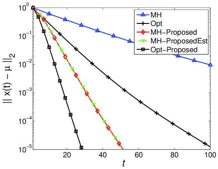
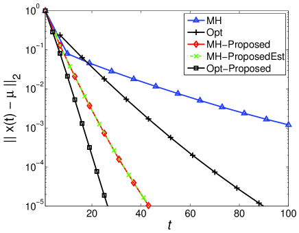
We first plot the MSE decay curves as a function of the number of consensus iterations $t$ for network size $N=200$, RGG topology and different initializations. Figure 1 compares the performance of the proposed algorithm with the algorithms using the MH or the optimal weight matrix of Xiao and Boyd [10]. It can be seen that our decentralized initialization scheme does not have a major influence on the performance of our approach, as the method initialized using a decentralized estimate for $\lambda_{2}(\mathbf{W})$ (the curve labelled MH-ProposedEst) and the method initialized using precise knowledge of $\lambda_{2}(\mathbf{W})$ (labelled MH-Proposed) coincide nearly exactly since the procedure discussed in Section III-D provides a good estimate of $\lambda_{2}(\mathbf{W})$ (to within $10^{-3}$ maximum relative error for a 200 node RGG). It is also clear that the proposed algorithm outperforms both the memoryless MH matrix and the optimal weight matrix of Xiao and Boyd [10]. In this experiment we fixed $K=2N$ and $L=10$. Note that the results in Figure 1 and all subsequent figures do not account for initialization costs. The initialization cost is relatively small. For the 200-node RGG it is equal to about $3N=600$ consensus iterations (if we bound the diameter of the 200-node RGG by 20). If we desire a relative error of $10^{-3}$, our algorithm gains approximately 70 iterations over memoryless MH consensus, based on Fig. 2(b). For this desired accuracy, the initialization overhead is thus recovered after less than 10 consensus operations.

(a) Slope initialization

(b) Spike initialization

Figure 1: MSE vs. iterations for 200-node random geometric graphs. The algorithms compared are: optimal weight matrix of Xiao and Boyd [10] (Opt): $+$; MH weights (MH): $\triangle$; proposed method with oracle $\lambda_{2}(\mathbf{W})$ and MH matrix (MH-Proposed): $\diamond$; proposed with decentralized estimate of $\lambda_{2}(\mathbf{W})$ (MH-ProposedEst): $\times$; accelerated consensus, with oracle $\lambda_{2}(\mathbf{W})$ and optimal matrix (Opt-Proposed): $\square$. (a) Slope initialization. (b) Spike initialization.

(a) Random geometric graph

(b) Chain

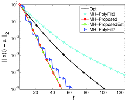
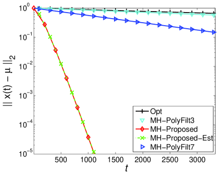
Figure 2: MSE vs. iteration for 200-node topologies, Slope initialization. The algorithms compared are: optimal weight matrix of Xiao and Boyd [10] (Opt): $+$; polynomial filter with 3 taps (MH-PolyFilt3): $\bigtriangledown$ and 7 taps (MH-PolyFilt7): $\triangleright$; proposed method with oracle $\lambda_{2}(\mathbf{W})$ and MH matrix (MH-Proposed): $\diamond$; proposed method with decentralized estiamte of $\lambda_{2}(\mathbf{W})$ (MH-ProposedEst): $\times$.

(a)

(b)

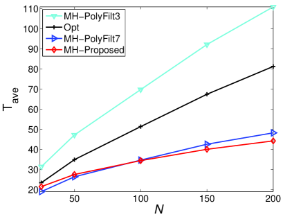
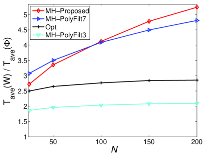
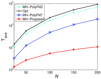
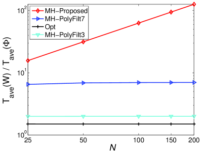
Figure 3: Averaging time characterization, random geometric graph topologies. The algorithms compared are: optimal weight matrix of Xiao and Boyd [10] (Opt): $+$; polynomial filter with 3 taps (MH-PolyFilt3): $\bigtriangledown$, and 7 taps (MH-PolyFilt7): $\triangleright$; proposed method with oracle $\lambda_{2}(\mathbf{W})$ and MH matrix (MH-Proposed): $\diamond$; proposed method with MH matrix and decentralized estimate of $\lambda_{2}(\mathbf{W})$ (MH-ProposedEst): $\times$. (a) Averaging time as a function of the network size. (b) Ratio of the averaging time of the non-accelerated algorithm to that of the associated accelerated algorithm.

(a)

(b)

Figure 4: Averaging time characterization, chain topology. The algorithms compared are: optimal weight matrix of Xiao and Boyd [10] (Opt): $+$; polynomial filter with 3 taps (MH-PolyFilt3): $\bigtriangledown$, and 7 taps (MH-PolyFilt7): $\triangleright$; proposed method with oracle $\lambda_{2}(\mathbf{W})$ and MH matrix (MH-Proposed): $\diamond$. (a) Averaging time as a function of the network size. (b) Improvement due to the accelerated consensus: ratio of the averaging time of the non-accelerated algorithm to that of the associated accelerated algorithm.

Figure 2 compares the MSE curves for the proposed algorithm with two versions of polynomial filtering consensus [14], one using 3 taps and the other using 7 taps. We see that in the RGG scenario, our algorithm outperforms polynomial filtering with $3$ memory taps and converges at a rate similar to that of the $7$-tap version of polynomial filtering. Decentralized calculation of topology-adapted polynomial filter weights also remains an open problem. We conclude that for random geometric graphs, our algorithm has superior properties with respect to polynomial filtering since it has better error performance for the same computational complexity, and our approach is suitable for completely distributed implementation. Moving our attention to the chain topology only emphasizes these points, as our accelerated algorithm significantly outperforms even 7-tap polynomial filtering. Note that decentralized initialization of our algorithm also works well in the chain graph scenario. However, to obtain this result we have to increase the number of consensus iterations in the eigenvalue estimation algorithm, $K$, from $2N$ to $N^{2}$. This increase in the complexity of the distributed optimization of accelerated consensus algorithm is due to the properties of the power methods [26] and related eigenvalue estimation problems. The accuracy of the second largest eigenvalue computation depends on the ratio $\lambda_{3}(\mathbf{W})/\lambda_{2}(\mathbf{W})$, and this ratio increases much more rapidly for the chain topology as $N$ grows than it does for random geometric graphs.

To investigate the robustness and scalability properties of the proposed algorithm, we next examine the averaging time, $T_{\scriptsize\mbox{ave}}(\mathbf{\Phi}_{3}[\alpha^{*}])$, as defined in (10), and the ratio $T_{\scriptsize\mbox{ave}}(\mathbf{W})/T_{\scriptsize\mbox{ave}}(\mathbf{\Phi}_{3}[\alpha^{*}])$, for random geometric graphs (Fig. 3) and the chain topology (Fig. 4). We establish through simulation that the scaling behaviour of the ratio that can be measured experimentally matches very well with the asymptotic result established theoretically for the processing gain, $\tau_{\textrm{asym}}(\mathbf{W})/\tau_{\textrm{asym}}(\mathbf{\Phi}_{3}[\alpha^{*}])$. We see from Fig. 3 that in the random geometric graph setting, the proposed algorithm always outperforms consensus with the optimal weight matrix of Xiao and Boyd [10] and polynomial filter with equal number of memory taps, and our approach scales comparably to 7-tap polynomial filtering. On the other hand, in the chain graph setting (Fig. 4) the proposed algorithm outperforms all the competing algorithms. Another interesting observation from Fig. 4 is that the gains of the polynomial filter and optimal weight matrix remain almost constant with varying network size while the gain obtained by the proposed algorithm increases significantly with $N$. This linear improvement with $N$ matches well with the asymptotic behavior predicted by Theorem 3.

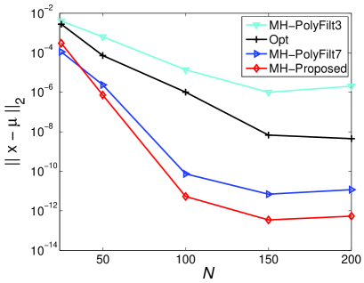
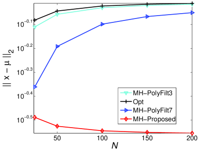
Finally, we compare the proposed algorithm with the linear observer approach of Sundaram and Hadjicostis [16], which works by remembering all of the consensus values, $x_{i}(t)$, seen at a node $i$ (unbounded memory). After enough updates, each node is able to perfectly recover the average by locally solving a set of linear equations. To compare the method of [16] with our approach and the other asymptotic approaches described above, we determine the topology-dependent number of iterations that the linear-observer method must execute to have enough information to exactly recover the average. We then run each of the asymptotic approaches for the same number of iterations and evaluate performance based on the MSE they achieve. Figure 5 depicts results for both random geometric graph and chain topologies. For random geometric graphs of $N\geq 100$ nodes, we observe that the proposed algorithm achieves an error of at most $10^{-12}$ (roughly machine precision), by the time the linear observer approach has sufficient information to compute the average. For the chain topology the results are much more favourable for the linear-observer approach. However, the linear observer approach requires significant overhead to determine the topology-dependent coefficients that define the linear system to be solved at each node and does not scale well to large networks.

(a) Random geometric graph

(b) Chain

Figure 5: MSE at the point when finite time consensus of Sundaram and Hadjicostis [16] has enough information to calculate the exact average at all nodes. The algorithms compared are: optimal weights (Opt): $+$; polynomial filter with 3 taps (MH-PolyFilt3): $\bigtriangledown$, and 7 taps (MH-PolyFilt7): $\triangleright$; proposed method with oracle $\lambda_{2}(\mathbf{W})$ and MH matrix (MH-Proposed): $\diamond$. (a) Random geometric graph. (b) Chain topology.

V Proofs of Main Results and Discussion

V-A Limiting $\varepsilon$-convergence time

To begin, we need to motivate choosing $\alpha$ to minimize the spectral radius $\rho(\mathbf{\Phi}_{3}[\alpha]-\mathbf{J})$ since, unlike in the memoryless setting, it does not bound the step-wise rate of convergence. In fact, since $\mathbf{\Phi}_{3}[\alpha]$ is not symmetric, $\mathbf{\Phi}_{3}[\alpha]^{t}$ does not even converge to $\mathbf{J}$ as $t\rightarrow\infty$, as in the memoryless setting. However, we will show that: (i) for the proposed construction, $\mathbf{\Phi}_{3}[\alpha]^{t}$ does converge to a matrix $\bar{\mathbf{\Phi}}$; (ii) that the limiting convergence time is governed by $\rho(\mathbf{\Phi}_{3}[\alpha]-\bar{\mathbf{\Phi}})$; and (iii) that $\rho(\mathbf{\Phi}_{3}[\alpha]-\bar{\mathbf{\Phi}})=\rho(\mathbf{\Phi}_{3}[\alpha]-\mathbf{J})$.

Before stating our first result we must introduce some notation. For now, assume we are given a matrix $\mathbf{\Phi}\in\mathbb{R}^{n\times n}$ with $\bar{\mathbf{\Phi}}=\lim_{t\rightarrow\infty}\mathbf{\Phi}^{t}$. We will address conditions for existence of the limit below. For a given initialization vector $\mathbf{x}(0)\in\mathbb{R}^{n}$, let $\tilde{\mathbf{x}}(0)=\bar{\mathbf{\Phi}}\mathbf{x}(0)$, and define the set of non-trivial initialization vectors $\mathcal{X}_{0,\mathbf{\Phi}}\triangleq\{\mathbf{x}(0)\in\mathbb{R}^{n}:\mathbf{x}(0)\neq\tilde{\mathbf{x}}(0)\}$. Since we have not yet established that $\tilde{\mathbf{x}}(0)=\bar{\mathbf{x}}(0)\triangleq\mathbf{J}\mathbf{x}(0)$, we keep the discussion general and use the following definition of the convergence time:

$$T_{\textrm{c}}(\mathbf{\Phi},\varepsilon)=\inf_{\tau\geq 0}\left\{\tau:||\mathbf{x}(t)-\tilde{\mathbf{x}}(0)||_{2}\leq\varepsilon||\mathbf{x}(0)-\tilde{\mathbf{x}}(0)||_{2}\quad\forall\ t\geq\tau,\quad\forall\ \mathbf{x}(0)\in\mathcal{X}_{0,\mathbf{\Phi}}\right\}$$ (16)

We now prove a result relating the spectral radius and the $\varepsilon$-convergence time for general non-symmetric averaging matrices $\mathbf{\Phi}$, which we will then apply to our particular construction, $\mathbf{\Phi}_{3}[\alpha]$.

Theorem 4.

Let $\mathbf{\Phi}\in\mathbb{R}^{n\times n}$ be given, with limit $\lim_{t\rightarrow\infty}\mathbf{\Phi}^{t}=\bar{\mathbf{\Phi}}$, and assume that $\rho(\mathbf{\Phi}-\bar{\mathbf{\Phi}})>0$. Then

$$\lim\limits_{\varepsilon\rightarrow 0}\frac{T_{\textrm{c}}(\mathbf{\Phi},\varepsilon)}{\log\varepsilon^{-1}}=\frac{1}{\log\rho(\mathbf{\Phi}-\bar{\mathbf{\Phi}})^{-1}}.$$ (17)

Proof:

The limit $\lim_{t\rightarrow\infty}\mathbf{\Phi}^{t}=\bar{\mathbf{\Phi}}$ exists if and only if (see [27]) $\mathbf{\Phi}$ can be expressed in the form

$$\mathbf{\Phi}={\mathbf{T}}\left[\begin{array}[]{cc}{\mathbf{I}}_{\kappa}&\mathbf{0}\\ \mathbf{0}&{\mathbf{Z}}\end{array}\right]{\mathbf{T}}^{-1}$$ (20)

where ${\mathbf{I}}_{\kappa}$ is the identity matrix of dimension $\kappa$, ${\mathbf{Z}}$ is a matrix with $\rho({\mathbf{Z}})<1$ and ${\mathbf{T}}$ is an invertible matrix. It follows that in the limit we have [15],

$$\bar{\mathbf{\Phi}}=\lim_{t\rightarrow\infty}\mathbf{\Phi}^{t}={\mathbf{T}}\left[\begin{array}[]{cc}{\mathbf{I}}_{\kappa}&\mathbf{0}\\ \mathbf{0}&\mathbf{0}\end{array}\right]{\mathbf{T}}^{-1}.$$ (23)

By linear algebra, $\mathbf{\Phi}\bar{\mathbf{\Phi}}=\bar{\mathbf{\Phi}}\mathbf{\Phi}=\bar{\mathbf{\Phi}}$ and $\mathbf{\Phi}^{t}\bar{\mathbf{\Phi}}=\bar{\mathbf{\Phi}}$. Using these facts it is trivial to show $(\mathbf{\Phi}-\bar{\mathbf{\Phi}})^{t}=\mathbf{\Phi}^{t}-\bar{\mathbf{\Phi}}$, implying $(\mathbf{\Phi}-\bar{\mathbf{\Phi}})^{t}(\mathbf{x}(0)-\tilde{\mathbf{x}}(0))=\mathbf{x}(t)-\tilde{\mathbf{x}}(0)$. Taking the norm of both sides we have

$$||\mathbf{x}(t)-\tilde{\mathbf{x}}(0)||_{2}=||(\mathbf{\Phi}-\bar{\mathbf{\Phi}})^{t}(\mathbf{x}(0)-\tilde{\mathbf{x}}(0))||_{2},$$ (24)

and therefore

$$T_{\textrm{c}}(\mathbf{\Phi},\varepsilon)=\inf_{\tau\geq 0}\left\{\tau:\frac{||(\mathbf{\Phi}-\bar{\mathbf{\Phi}})^{t}(\mathbf{x}(0)-\tilde{\mathbf{x}}(0))||_{2}}{||\mathbf{x}(0)-\tilde{\mathbf{x}}(0)||_{2}}\leq\varepsilon\quad\forall\ t\geq\tau,\quad\forall\ \mathbf{x}(0)\in\mathcal{X}_{0,\mathbf{\Phi}}\right\}.$$ (25)

By the definition of $T_{\textrm{c}}(\mathbf{\Phi},\varepsilon)$ above we have:

$$\frac{||(\mathbf{\Phi}-\bar{\mathbf{\Phi}})^{T_{\textrm{c}}(\mathbf{\Phi},\varepsilon)}(\mathbf{x}(0)-\tilde{\mathbf{x}}(0))||_{2}}{||\mathbf{x}(0)-\tilde{\mathbf{x}}(0)||_{2}}\leq\varepsilon,\quad\forall\mathbf{x}(0)\in\mathcal{X}_{0,\mathbf{\Phi}}.$$ (26)

This implies:

$$\left[\left(\sup\limits_{\mathbf{x}(0)\in\mathcal{X}_{0,\mathbf{\Phi}}}\frac{||(\mathbf{\Phi}-\bar{\mathbf{\Phi}})^{T_{\textrm{c}}(\mathbf{\Phi},\varepsilon)}(\mathbf{x}(0)-\tilde{\mathbf{x}}(0))||_{2}}{||\mathbf{x}(0)-\tilde{\mathbf{x}}(0)||_{2}}\right)^{1/T_{\textrm{c}}(\mathbf{\Phi},\varepsilon)}\right]^{T_{\textrm{c}}(\mathbf{\Phi},\varepsilon)}\leq\varepsilon,$$ (27)

and so, using the definition of the induced operator norm, which is simply $||\mathbf{\Phi}-\bar{\mathbf{\Phi}}||_{2}=\sup_{\mathbf{x}(0)\in\mathcal{X}_{0,\mathbf{\Phi}}}||(\mathbf{\Phi}-\bar{\mathbf{\Phi}})(\mathbf{x}(0)-\tilde{\mathbf{x}}(0))||_{2}/||\mathbf{x}(0)-\tilde{\mathbf{x}}(0)||_{2}$, after taking the logarithm on both sides of (27), we have

$$T_{\textrm{c}}(\mathbf{\Phi},\varepsilon) \geq\frac{\log\varepsilon}{\log||(\mathbf{\Phi}-\bar{\mathbf{\Phi}})^{T_{\textrm{c}}(\mathbf{\Phi},\varepsilon)}||_{2}^{1/{T_{\textrm{c}}(\mathbf{\Phi},\varepsilon)}}}.$$ (28)

Since [23] $\rho(\mathbf{\Phi}-\bar{\mathbf{\Phi}})\leq||(\mathbf{\Phi}-\bar{\mathbf{\Phi}})^{t}||_{2}^{1/t}$ for any $t\geq 0$, it follows that

$$T_{\textrm{c}}(\mathbf{\Phi},\varepsilon) \geq\frac{\log\varepsilon}{\log\rho(\mathbf{\Phi}-\bar{\mathbf{\Phi}})}.$$ (29)

from which it is also clear that $T_{\textrm{c}}(\mathbf{\Phi},\varepsilon)\rightarrow\infty$ as $\varepsilon\rightarrow 0$.

Now, by the definition of $T_{\textrm{c}}(\mathbf{\Phi},\varepsilon)$ in (25) we also have

$$\exists\mathbf{x}(0)\in\mathcal{X}_{0,\mathbf{\Phi}},\quad\frac{||(\mathbf{\Phi}-\bar{\mathbf{\Phi}})^{T_{\textrm{c}}(\mathbf{\Phi},\varepsilon)-1}(\mathbf{x}(0)-\tilde{\mathbf{x}}(0))||_{2}}{||\mathbf{x}(0)-\tilde{\mathbf{x}}(0)||_{2}}>\varepsilon,$$ (30)

implying, for the operator norm of $(\mathbf{\Phi}-\bar{\mathbf{\Phi}})^{T_{\textrm{c}}(\mathbf{\Phi},\varepsilon)-1}$:

$$||(\mathbf{\Phi}-\bar{\mathbf{\Phi}})^{T_{\textrm{c}}(\mathbf{\Phi},\varepsilon)-1}||_{2}>\varepsilon.$$ (31)

From (31) and (27) it follows $||(\mathbf{\Phi}-\bar{\mathbf{\Phi}})^{T_{\textrm{c}}(\mathbf{\Phi},\varepsilon)}||_{2}\leq\varepsilon<||(\mathbf{\Phi}-\bar{\mathbf{\Phi}})^{T_{\textrm{c}}(\mathbf{\Phi},\varepsilon)-1}||_{2}$ and thus we can always pick $\beta\in[0,1)$ such that the following holds:

$$\beta||(\mathbf{\Phi}-\bar{\mathbf{\Phi}})^{T_{\textrm{c}}(\mathbf{\Phi},\varepsilon)-1}||_{2}+(1-\beta)||(\mathbf{\Phi}-\bar{\mathbf{\Phi}})^{T_{\textrm{c}}(\mathbf{\Phi},\varepsilon)}||_{2}=\varepsilon.$$ (32)

Using the notation $C_{T_{\textrm{c}}}=||(\mathbf{\Phi}-\bar{\mathbf{\Phi}})^{T_{\textrm{c}}(\mathbf{\Phi},\varepsilon)}||_{2}/||(\mathbf{\Phi}-\bar{\mathbf{\Phi}})^{T_{\textrm{c}}(\mathbf{\Phi},\varepsilon)-1}||_{2}$ for the bounded number $C_{T_{\textrm{c}}}$ we conclude

$$||(\mathbf{\Phi}-\bar{\mathbf{\Phi}})^{T_{\textrm{c}}(\mathbf{\Phi},\varepsilon)-1}||_{2}(\beta+(1-\beta)C_{T_{\textrm{c}}})=\varepsilon.$$ (33)

The boundedness of $C_{T_{\textrm{c}}}$ follows from the sub-multiplicativity of the operator norm, $||(\mathbf{\Phi}-\bar{\mathbf{\Phi}})^{T_{\textrm{c}}(\mathbf{\Phi},\varepsilon)}||_{2}\leq\|\mathbf{\Phi}-\bar{\mathbf{\Phi}}\|_{2}||(\mathbf{\Phi}-\bar{\mathbf{\Phi}})^{T_{\textrm{c}}(\mathbf{\Phi},\varepsilon)-1}||_{2}$ yielding $0\leq C_{T_{\textrm{c}}}\leq\|\mathbf{\Phi}-\bar{\mathbf{\Phi}}\|_{2}$.

Using the technique used to switch from (27) to (28) we obtain from (33):

$$(T_{\textrm{c}}(\mathbf{\Phi},\varepsilon)-1)\log||(\mathbf{\Phi}-\bar{\mathbf{\Phi}})^{T_{\textrm{c}}(\mathbf{\Phi},\varepsilon)-1}||_{2}^{1/(T_{\textrm{c}}(\mathbf{\Phi},\varepsilon)-1)}=\log\varepsilon-\log(\beta+(1-\beta)C_{T_{\textrm{c}}}).$$ (34)

Dividing through by $\log\varepsilon^{-1}\log||(\mathbf{\Phi}-\bar{\mathbf{\Phi}})^{T_{\textrm{c}}(\mathbf{\Phi},\varepsilon)-1}||_{2}^{1/(T_{\textrm{c}}(\mathbf{\Phi},\varepsilon)-1)}$, and taking the limit as $\varepsilon\rightarrow 0$ we have

$$\lim\limits_{\varepsilon\rightarrow 0}\frac{T_{\textrm{c}}(\mathbf{\Phi},\varepsilon)}{\log\varepsilon^{-1}} =\lim\limits_{\varepsilon\rightarrow 0}\frac{-1}{\log||(\mathbf{\Phi}-\bar{\mathbf{\Phi}})^{T_{\textrm{c}}(\mathbf{\Phi},\varepsilon)-1}||_{2}^{1/(T_{\textrm{c}}(\mathbf{\Phi},\varepsilon)-1)}}$$

$$-\lim\limits_{\varepsilon\rightarrow 0}\frac{\log(\beta+(1-\beta)C_{T_{\textrm{c}}})}{\log||(\mathbf{\Phi}-\bar{\mathbf{\Phi}})^{T_{\textrm{c}}(\mathbf{\Phi},\varepsilon)-1}||_{2}^{1/(T_{\textrm{c}}(\mathbf{\Phi},\varepsilon)-1)}\log\varepsilon^{-1}}+\lim\limits_{\varepsilon\rightarrow 0}\frac{1}{\log\varepsilon^{-1}}.$$ (35)

Moving the limits on the right under the logs and using the fact that $T_{\textrm{c}}(\mathbf{\Phi},\varepsilon)\rightarrow\infty$ as $\varepsilon\rightarrow 0$, we may employ Gelfand’s formula [23], $\lim_{t\rightarrow\infty}||(\mathbf{\Phi}-\bar{\mathbf{\Phi}})^{t}||^{1/t}=\rho(\mathbf{\Phi}-\bar{\mathbf{\Phi}})$:

$$\lim\limits_{\varepsilon\rightarrow 0}\frac{T_{\textrm{c}}(\mathbf{\Phi},\varepsilon)}{\log\varepsilon^{-1}} =\frac{-1}{\log\lim\limits_{\varepsilon\rightarrow 0}||(\mathbf{\Phi}-\bar{\mathbf{\Phi}})^{T_{\textrm{c}}(\mathbf{\Phi},\varepsilon)-1}||_{2}^{1/(T_{\textrm{c}}(\mathbf{\Phi},\varepsilon)-1)}}-\lim\limits_{\varepsilon\rightarrow 0}\frac{\log(\beta+(1-\beta)C_{T_{\textrm{c}}})}{\log\lim\limits_{\varepsilon\rightarrow 0}||(\mathbf{\Phi}-\bar{\mathbf{\Phi}})^{T_{\textrm{c}}(\mathbf{\Phi},\varepsilon)-1}||_{2}^{1/(T_{\textrm{c}}(\mathbf{\Phi},\varepsilon)-1)}\log\varepsilon^{-1}}$$

$$=\frac{1}{\log\rho(\mathbf{\Phi}-\bar{\mathbf{\Phi}})^{-1}}+\lim\limits_{\varepsilon\rightarrow 0}\frac{\log(\beta+(1-\beta)C_{T_{\textrm{c}}})}{\log\rho(\mathbf{\Phi}-\bar{\mathbf{\Phi}})^{-1}\log\varepsilon^{-1}}$$ (36)

Using $C_{T_{\textrm{c}}}\leq\|\mathbf{\Phi}-\bar{\mathbf{\Phi}}\|$, $\log(\beta+(1-\beta)C_{T_{\textrm{c}}})\leq|\log(\beta+(1-\beta)\|\mathbf{\Phi}-\bar{\mathbf{\Phi}}\|)|$, and taking into account the fact that $0\leq|\log(\beta+(1-\beta)\|\mathbf{\Phi}-\bar{\mathbf{\Phi}}\|)|\leq|\log\|\mathbf{\Phi}-\bar{\mathbf{\Phi}}\||,\ \forall\beta\in[0,1],$ we have

$$\lim\limits_{\varepsilon\rightarrow 0}\frac{T_{\textrm{c}}(\mathbf{\Phi},\varepsilon)}{\log\varepsilon^{-1}} \leq\frac{1}{\log\rho(\mathbf{\Phi}-\bar{\mathbf{\Phi}})^{-1}}+\lim\limits_{\varepsilon\rightarrow 0}\frac{|\log(\|\mathbf{\Phi}-\bar{\mathbf{\Phi}}\|)|}{\log\rho(\mathbf{\Phi}-\bar{\mathbf{\Phi}})^{-1}\log\varepsilon^{-1}}$$

$$=\frac{1}{\log\rho(\mathbf{\Phi}-\bar{\mathbf{\Phi}})^{-1}}$$ (37)

Combining the last inequality with (29) completes the proof. ∎

In order to apply the above result, we must establish that $\mathbf{\Phi}_{3}[\alpha]$ satisfies the conditions of Theorem 4. In doing so, we will also show that (i) for $\mathbf{\Phi}=\mathbf{\Phi}_{3}[\alpha]$ and $\mathbf{X}(0)$ defined in (6), the limit $\bar{\mathbf{\Phi}}\mathbf{X}(0)=\mathbf{J}\mathbf{X}(0)$, so our approach indeed converges to the average consensus, and (ii) that the limiting convergence time is characterized by a function of $\rho(\mathbf{\Phi}_{3}[\alpha]-\mathbf{J})$, which motivates choosing $\alpha$ to optimize this expression. (Recall, in this setting $\mathbf{J}$ is the $2N\times 2N$ matrix with all entries equal to $1/2N$.) Note that the condition on $\alpha$ is necessary for $\mathbf{\Phi}_{3}[\alpha]^{t}$ to have a limit as $t\rightarrow\infty$, as will be established in Section V-B.

Proposition 1.

Let $\mathbf{\Phi}_{3}[\alpha]$ be defined as in (7), assume that the assumptions of Theorem 1 hold, and $\alpha\in[0,-\theta_{1}^{-1})$. Then:

(a)

$\bar{\mathbf{\Phi}}_{3}[\alpha]=\lim_{t\rightarrow\infty}\mathbf{\Phi}_{3}[\alpha]^{t}$ exists, with $\bar{\mathbf{\Phi}}_{3}[\alpha]\mathbf{X}(0)=\mathbf{J}\mathbf{X}(0)$ for all $\mathbf{X}(0)$ defined in (6),

(b)

$\rho(\mathbf{\Phi}_{3}[\alpha]-\bar{\mathbf{\Phi}}_{3}[\alpha])>0$, and

(c)

$\lim\limits_{\varepsilon\rightarrow 0}\frac{T_{\textrm{c}}(\mathbf{\Phi}_{3}[\alpha],\varepsilon)}{\log\varepsilon^{-1}}=\frac{1}{\log\rho(\mathbf{\Phi}_{3}[\alpha]-{\mathbf{J}})^{-1}}.$

Proof:

Proof of part (a). In Theorem 1 in [15], Johansson and Johansson show that the necessary and sufficient conditions for the consensus algorithm of the form $\mathbf{\Phi}_{3}[\alpha]$ to converge to the average are (JJ1) $\mathbf{\Phi}_{3}[\alpha]{\bm{1}}={\bm{1}}$; (JJ2) $\mathbf{g}^{T}\mathbf{\Phi}_{3}[\alpha]=\mathbf{g}^{T}$ for vector $\mathbf{g}^{T}=[\beta_{1}{\bm{1}}^{T}\beta_{2}{\bm{1}}^{T}]$ with weights satisfying $\beta_{1}+\beta_{2}=1$; and (JJ3) $\rho(\mathbf{\Phi}_{3}[\alpha]-\frac{1}{N}{\bm{1}}\mathbf{g}^{T})<1$. If these conditions hold then we also have $\bar{\mathbf{\Phi}}_{3}[\alpha]=\frac{1}{N}{\bm{1}}\mathbf{g}^{T}$ [15] implying $\tilde{\mathbf{X}}(0)=\bar{\mathbf{X}}(0)$. Condition (JJ1) is easily verified after straightforward algebraic manipulations using the definition of $\mathbf{\Phi}_{3}[\alpha]$ in (7), the assumption that $\theta_{1}+\theta_{2}+\theta_{3}=1$, and recalling that $\mathbf{W}$ satisfies $\mathbf{W}{\bm{1}}={\bm{1}}$ by design. To address condition (JJ2), we set $\beta_{1}=1/(1+\alpha\theta_{1})$ and $\beta_{2}=\alpha\theta_{1}/(1+\alpha\theta_{1})$. Clearly, $\beta_{1}+\beta_{2}=1$, and it is also easy to verify condition (JJ2) by plugging these values into the definition of $\mathbf{g}$, and using the same properties of $\mathbf{\Phi}_{3}[\alpha]$, the $\theta_{i}$’s, and $\mathbf{W}$ as above.

In order to verify that condition (JJ3) holds, we will show here that $\rho(\mathbf{\Phi}_{3}[\alpha]-\frac{1}{N}{\bm{1}}\mathbf{g}^{T})=\rho(\mathbf{\Phi}_{3}[\alpha]-\mathbf{J})$. In Section V-B we show that $\rho(\mathbf{\Phi}_{3}[\alpha]-\mathbf{J})<1$ if $\alpha\in[0,-\theta_{1}^{-1})$, and thus condition (JJ3) is also satisfied under the assumptions of the proposition. To show that $\rho(\mathbf{\Phi}_{3}[\alpha]-\frac{1}{N}{\bm{1}}\mathbf{g}^{T})=\rho(\mathbf{\Phi}_{3}[\alpha]-\mathbf{J})$, we prove a stronger result, namely that $\mathbf{\Phi}_{3}[\alpha]-\frac{1}{N}{\bm{1}}\mathbf{g}^{T}$ and $\mathbf{\Phi}_{3}[\alpha]-\mathbf{J}$ have the same eigenspectra. Consider the eigenvector $\mathbf{v}_{i}$ of $\mathbf{\Phi}_{3}[\alpha]$ with corresponding eigenvalue $\lambda_{i}(\mathbf{\Phi}_{3}[\alpha])$. This pair solves the eigenvalue problem, $\mathbf{\Phi}_{3}[\alpha]\mathbf{v}_{i}=\lambda_{i}(\mathbf{\Phi}_{3}[\alpha])\mathbf{v}_{i}$. Equivalently, expanding the definition of $\mathbf{\Phi}_{3}[\alpha]$, we have

$$\left[\begin{array}[]{cc}\mathbf{W}_{3}[\alpha]&\alpha\theta_{1}\mathbf{I}\\ \mathbf{I}&\mathbf{0}\end{array}\right]\mathbf{v}_{i}=\lambda_{i}(\mathbf{\Phi}_{3}[\alpha])\left[\begin{array}[]{cc}\mathbf{I}&\mathbf{0}\\ \mathbf{0}&\mathbf{I}\end{array}\right]\mathbf{v}_{i}.$$ (42)

We observe that (42) fits a modification of the first companion form of the linearization of a Quadratic Eigenvalue Problem (QEP) (see Section 3.4 in [28]). The QEP has general form $(\lambda^{2}\mathbf{M}+\lambda\mathbf{C}+\mathbf{K})\mathbf{u}=\mathbf{0}$, where $\mathbf{u}$ is the eigenvector associated with this QEP. The linearization of interest to us has the form:

$$\left[\begin{array}[]{cc}-\mathbf{C}&-\mathbf{K}\\ \mathbf{I}&\mathbf{0}\end{array}\right]\left[\begin{array}[]{c}\lambda{\mathbf{u}}\\ {\mathbf{u}}\end{array}\right]-\lambda\left[\begin{array}[]{cc}\mathbf{M}&\mathbf{0}\\ \mathbf{0}&\mathbf{I}\end{array}\right]\left[\begin{array}[]{c}\lambda{\mathbf{u}}\\ {\mathbf{u}}\end{array}\right]=\mathbf{0}.$$ (51)

The correspondence is clear if we make the associations: $\mathbf{M}=\mathbf{I}$, $\mathbf{C}=-\mathbf{W}_{3}[\alpha]$ and $\mathbf{K}=-\alpha\theta_{1}\mathbf{I}$, $\lambda=\lambda_{i}(\mathbf{\Phi}_{3}[\alpha])$ and $\mathbf{v}_{i}=[\lambda_{i}(\mathbf{\Phi}_{3}[\alpha]){\mathbf{u}}^{T}{\mathbf{u}}^{T}]^{T}$. Eigenvectors $\mathbf{v}_{i}$ that solve (42) thus have special structure and are related to $\mathbf{u}_{i}$, the solution to the QEP,

$$(\lambda_{i}(\mathbf{\Phi}_{3}[\alpha])^{2}\mathbf{I}-\lambda_{i}(\mathbf{\Phi}_{3}[\alpha])\mathbf{W}_{3}[\alpha]-\alpha\theta_{1}\mathbf{I})\mathbf{u}_{i}=\mathbf{0}.$$ (52)

Because the first and third terms above are scaled identity matrices and the definition of $\mathbf{W}_{3}[\alpha]$ (see (5)) also involves scaled identity matrices, we can simplify this last equation to find that any solution $\mathbf{u}_{i}$ must also be an eigenvector of $\mathbf{W}$.

We have seen above, when verifying condition (JJ1), that ${\bm{1}}$ is an eigenvector of $\mathbf{\Phi}_{3}[\alpha]$ with corresponding eigenvalue $\lambda_{i}(\mathbf{\Phi}_{3}[\alpha])=1$. Observe that, from the definition of $\mathbf{g}$ and because $\beta_{1}+\beta_{2}=1$, we have $(\frac{1}{N}{\bm{1}}\mathbf{g}^{T}){\bm{1}}={\bm{1}}$. Thus, $(\mathbf{\Phi}_{3}[\alpha]-\frac{1}{N}{\bm{1}}\mathbf{g}^{T}){\bm{1}}=\mathbf{0}$. Similarly, recalling that $\mathbf{J}=\frac{1}{2N}{\bm{1}}{\bm{1}}^{T}$, we have $\mathbf{J}{\bm{1}}={\bm{1}}$, and thus $(\mathbf{\Phi}_{3}[\alpha]-\mathbf{J}){\bm{1}}=\mathbf{0}$. By design, $\mathbf{W}$ is a doubly stochastic matrix, and all eigenvectors $\mathbf{u}$ of $\mathbf{W}$ with $\mathbf{u}\neq{\bm{1}}$ are orthogonal to ${\bm{1}}$. It follows that $(\frac{1}{N}{\bm{1}}\mathbf{g}^{T})\mathbf{v}_{i}=\mathbf{0}$ for corresponding eigenvectors $\mathbf{v}_{i}=[\lambda_{i}(\mathbf{\Phi}_{3}[\alpha])\mathbf{u}^{T}\mathbf{u}^{T}]^{T}$ of $\mathbf{\Phi}_{3}[\alpha]$, and thus $(\mathbf{\Phi}_{3}[\alpha]-\frac{1}{N}{\bm{1}}\mathbf{g}^{T})\mathbf{v}_{i}=\mathbf{\Phi}_{3}[\alpha]\mathbf{v}_{i}=\lambda_{i}(\mathbf{\Phi}_{3}[\alpha])\mathbf{v}_{i}$. Similarly, $\mathbf{J}\mathbf{v}_{i}=0$ if $\mathbf{v}_{i}\neq{\bm{1}}$, and $(\mathbf{\Phi}_{3}[\alpha]-\mathbf{J})\mathbf{v}_{i}=\lambda_{i}(\mathbf{\Phi}_{3}[\alpha])\mathbf{v}_{i}$. Therefore, we conclude that the matrices $(\mathbf{\Phi}_{3}[\alpha]-\bar{\mathbf{\Phi}}_{3}[\alpha])$ and $(\mathbf{\Phi}_{3}[\alpha]-\mathbf{J})$ have identical eigenspectra, and thus $\rho(\mathbf{\Phi}_{3}[\alpha]-\frac{1}{N}{\bm{1}}\mathbf{g}^{T})=\rho(\mathbf{\Phi}_{3}[\alpha]-\mathbf{J})$.

In Section V-B we show that $\rho(\mathbf{\Phi}_{3}[\alpha]-\mathbf{J})<1$ if $\alpha\in[0,-\theta_{1}^{-1})$, and thus the assumptions of the proposition, taken together with the analysis just conducted, verify that condition (JJ3) is also satisfied. Therefore, the limit $\lim_{t\rightarrow\infty}\mathbf{\Phi}_{3}[\alpha]^{t}=\bar{\mathbf{\Phi}}_{3}[\alpha]=\frac{1}{N}{\bm{1}}\mathbf{g}^{T}$ exists, and $\bar{\mathbf{\Phi}}_{3}[\alpha]\mathbf{X}(0)=\mathbf{J}\mathbf{X}(0)$ for all $\mathbf{X}(0)$ defined in (6).

Proofs of parts (b) and (c). In the proof of Lemma 1 (see Section V-B), it is shown that $\rho(\mathbf{\Phi}_{3}[\alpha]-{\mathbf{J}}])\geq-\alpha\theta_{1}$. Thus, if $\alpha>0$ and $\theta_{1}<0$, then part (b) holds. The assumptions $\theta_{1}+\theta_{2}+\theta_{3}=1$, $\theta_{3}\geq 1$, and $\theta_{2}\geq 0$ imply that $\theta_{1}\leq 0$, and by assumption, $\alpha\geq 0$. If $\alpha=0$ or $\theta_{1}=0$, then the proposed predictive consensus scheme reduces to memoryless consensus with weight matrix $\mathbf{W}$ (and the statement follows directly from the results of [10, 11]). Thus, part (b) of the proposition follows from the assumptions and the analysis in Lemma 1 below. By proving parts (a) and (b), we have verified the assumptions of Theorem 4 above. Applying the result of this Theorem, together with the equivalence of $\rho(\mathbf{\Phi}_{3}[\alpha]-\frac{1}{N}{\bm{1}}\mathbf{g}^{T})$ and $\rho(\mathbf{\Phi}_{3}[\alpha]-\mathbf{J})$, gives the claim in part (c), thereby completing the proof. ∎

V-B Proof of Theorem 1: Optimal Mixing Parameter

In order to minimize the spectral radius of $\mathbf{\Phi}_{3}[\alpha]$ we need to know its eigenvalues. These can be calculated by solving the eigenvalue problem (42). We can multiply (52) by $\mathbf{u}^{T}_{i}$ on the left to obtain a quadratic equation that links the individual eigenvalues $\lambda_{i}(\mathbf{\Phi}_{3}[\alpha])$ and $\lambda_{i}(\mathbf{W}_{3}[\alpha])$:

$$\mathbf{u}_{i}^{T}(\lambda_{i}(\mathbf{\Phi}_{3}[\alpha])^{2}\mathbf{I}-\lambda_{i}(\mathbf{\Phi}_{3}[\alpha])\mathbf{W}_{3}[\alpha]-\alpha\theta_{1}\mathbf{I})\mathbf{u}_{i} =0$$

$$\lambda_{i}(\mathbf{\Phi}_{3}[\alpha])^{2}-\lambda_{i}(\mathbf{W}_{3}[\alpha])\lambda_{i}(\mathbf{\Phi}_{3}[\alpha])-\alpha\theta_{1} =0.$$ (53)

Recall $\mathbf{\Phi}_{3}[\alpha]$ is a $2N\times 2N$ matrix, and so $\mathbf{\Phi}_{3}[\alpha]$ has, in general, $2N$ eigenvalues – twice as many as $\mathbf{W}_{3}[\alpha]$. These eigenvalues are the solutions of the quadratic (V-B), and are given by

$$\lambda_{i}^{*}(\mathbf{\Phi}_{3}[\alpha]) =\frac{1}{2}\left(\lambda_{i}(\mathbf{W}_{3}[\alpha])+\sqrt{\lambda_{i}(\mathbf{W}_{3}[\alpha])^{2}+4\alpha\theta_{1}}\right)$$

$$\lambda_{i}^{**}(\mathbf{\Phi}_{3}[\alpha]) =\frac{1}{2}\left(\lambda_{i}(\mathbf{W}_{3}[\alpha])-\sqrt{\lambda_{i}(\mathbf{W}_{3}[\alpha])^{2}+4\alpha\theta_{1}}\right).$$ (54)

With these expressions for the eigenvalues of $\mathbf{\Phi}_{3}[\alpha]$, we are in a position to formulate the problem of minimizing the spectral radius of the matrix $(\mathbf{\Phi}_{3}[\alpha]-\mathbf{J})$, $\alpha^{\star}=\arg\min\limits_{\alpha}\rho(\mathbf{\Phi}_{3}[\alpha]-\mathbf{J})$. It can be shown that this problem is equivalent to

$$\alpha^{\star}=\arg\min\limits_{\alpha\geq 0}\rho(\mathbf{\Phi}_{3}[\alpha]-\mathbf{J})$$ (55)

The simplest way to demonstrate this is to show that $\rho(\mathbf{\Phi}_{3}[\alpha]-\mathbf{J})\geq\rho(\mathbf{\Phi}_{3}[0]-\mathbf{J})$ for any $\alpha<0$. Indeed, by the definition of the spectral radius we have that $\rho(\mathbf{\Phi}_{3}[\alpha]-\mathbf{J})\geq\lambda_{2}^{*}(\mathbf{\Phi}_{3}[\alpha])$ and $\rho(\mathbf{\Phi}_{3}[0]-\mathbf{J})=\lambda_{2}(\mathbf{W})$. The latter is clear if we plug $\alpha=0$ into (V-B). Hence it is enough to demonstrate $\lambda_{2}^{*}(\mathbf{\Phi}_{3}[\alpha])\geq\lambda_{2}(\mathbf{W})$. Consider the inequality $\lambda_{2}^{*}(\mathbf{\Phi}_{3}[\alpha])-\lambda_{2}(\mathbf{W})\geq 0.$ Replacing $\lambda_{2}^{*}(\mathbf{\Phi}_{3}[\alpha])$ with its definition according to (V-B), rearranging terms and squaring both sides gives $\alpha\theta_{1}\geq\lambda_{2}(\mathbf{W})^{2}-\lambda_{2}(\mathbf{W})\lambda_{2}(\mathbf{W}_{3}[\alpha])$. From the definition of $\mathbf{W}_{3}[\alpha]$ in (5), it follows that $\lambda_{2}(\mathbf{W}_{3}[\alpha])=(1-\alpha+\alpha\theta_{3})\lambda_{2}(\mathbf{W})+\alpha\theta_{2}$. Using this relation leads to the expression $\alpha(\theta_{1}+(\theta_{3}-1)\lambda_{2}(\mathbf{W})^{2}+\theta_{2}\lambda_{2}(\mathbf{W}))\geq 0$. Under our assumptions, we have $\theta_{3}-1\geq 0$, $\theta_{2}\geq 0$ and $\theta_{1}\leq 0$. Thus $\theta_{1}+(\theta_{3}-1)\lambda_{2}(\mathbf{W})^{2}+\theta_{2}\lambda_{2}(\mathbf{W})\leq\theta_{1}+\theta_{3}-1+\theta_{2}=0$ since $\lambda_{2}(\mathbf{W})<1$. This implies that if $\alpha<0$, the last inequality holds leading to $\lambda_{2}^{*}(\mathbf{\Phi}_{3}[\alpha])\geq\lambda_{2}(\mathbf{W})$. Thus for any $\alpha<0$ the spectral radius $\rho(\mathbf{\Phi}_{3}[\alpha]-\mathbf{J})$ cannot decrease, and so we may focus on optimizing over $\alpha\geq 0$.

Now, the proof of Theorem 1 boils down to examining how varying $\alpha$ affects the eigenvalues of $\mathbf{\Phi}_{3}[\alpha]$ on a case-by-case basis. We first show that the first eigenvalues, $\lambda^{*}_{1}(\mathbf{\Phi}_{3}[\alpha])$ and $\lambda^{**}_{1}(\mathbf{\Phi}_{3}[\alpha])$, are smaller than all the others. Then, we demonstrate that the second eigenvalues, $\lambda^{*}_{2}(\mathbf{\Phi}_{3}[\alpha])$ and $\lambda^{**}_{2}(\mathbf{\Phi}_{3}[\alpha])$, dominate all other pairs, $\lambda^{*}_{j}(\mathbf{\Phi}_{3}[\alpha])$ and $\lambda^{**}_{j}(\mathbf{\Phi}_{3}[\alpha])$, for $j>2$, allowing us to focus on the second eigenvalues, from which the proof follows. Along the way, we establish conditions on $\alpha$ which guarantee stability of the proposed two-tap predictive consensus methodology.

To begin, we reformulate the optimization problem in terms of the eigenvalues of $\mathbf{\Phi}_{3}[\alpha]$. We first consider $\lambda_{1}^{*}(\mathbf{\Phi}_{3}[\alpha])$ and $\lambda_{1}^{**}(\mathbf{\Phi}_{3}[\alpha])$. Substituting $\lambda_{1}(\mathbf{W}_{3}[\alpha])=(1-\alpha+\alpha\theta_{3})+\alpha\theta_{2}$ we obtain the relationship $\sqrt{\lambda^{2}_{1}(\mathbf{W}_{3}[\alpha])+4\alpha\theta_{1}}=|1+\alpha\theta_{1}|$ and using the condition $\theta_{1}\leq 0$, we conclude that

$$\lambda_{1}^{*}(\mathbf{\Phi}_{3}[\alpha]),\lambda_{1}^{**}(\mathbf{\Phi}_{3}[\alpha]) =\left\{\begin{array}[]{cc}1,-\alpha\theta_{1}&\textrm{if \ }1+\alpha\theta_{1}\geq 0\Rightarrow\alpha\leq-\theta_{1}^{-1}\\ -\alpha\theta_{1},1&\textrm{if \ }1+\alpha\theta_{1}<0\Rightarrow\alpha>-\theta_{1}^{-1}.\end{array}\right.$$ (58)

We note that $\alpha>-\theta_{1}^{-1}$ implies $|\lambda_{1}^{**}(\mathbf{\Phi}_{3}[\alpha])|>1$, leading to divergence of the linear recursion involving $\mathbf{\Phi}_{3}[\alpha]$, and thus conclude that the potential solution is restricted to the range $\alpha\leq-\theta_{1}^{-1}$. Focusing on this setting, we write $\lambda_{1}^{*}(\mathbf{\Phi}_{3}[\alpha])=1$ and $\lambda_{1}^{**}(\mathbf{\Phi}_{3}[\alpha])=-\alpha\theta_{1}$. We can now reformulate the problem (55) in terms of the eigenvalues of $\mathbf{\Phi}_{3}[\alpha]$:

$$\alpha^{\star}=\arg\min\limits_{\alpha\geq 0}\max\limits_{i=1,2,\ldots N}\mathcal{J}_{i}[\alpha,\lambda_{i}(\mathbf{W})]$$ (59)

where

$$\mathcal{J}_{i}[\alpha,\lambda_{i}(\mathbf{W})]=\begin{cases}|\lambda_{1}^{**}(\mathbf{\Phi}_{3}[\alpha])|,&i=1\\ \max(|\lambda_{i}^{*}(\mathbf{\Phi}_{3}[\alpha])|,|\lambda_{i}^{**}(\mathbf{\Phi}_{3}[\alpha])|)&i>1.\end{cases}$$ (60)

We now state a lemma that characterizes the functions $\mathcal{J}_{i}[\alpha,\lambda_{i}(\mathbf{W})]$.

Lemma 1.

Under the assumptions of Theorem 1,

$$\mathcal{J}_{i}[\alpha,\lambda_{i}(\mathbf{W})] =\left\{\begin{array}[]{cc}\alpha^{1/2}(-\theta_{1})^{1/2}&\textrm{if \ }\alpha\in[\alpha^{*}_{i},\theta_{1}^{-1}]\\ \frac{1}{2}\left(\left|\lambda_{i}(\mathbf{W}_{3}[\alpha])\right|+\sqrt{\lambda_{i}(\mathbf{W}_{3}[\alpha])^{2}+4\alpha\theta_{1}}\right)&\textrm{if \ }\alpha\in[0,\alpha^{*}_{i})\end{array}\right.$$ (63)

where

$$\alpha^{*}_{i}=\frac{-((\theta_{3}-1)\lambda_{i}(\mathbf{W})^{2}+\theta_{2}\lambda_{i}(\mathbf{W})+2\theta_{1})-2\sqrt{\theta_{1}^{2}+\theta_{1}\lambda_{i}(\mathbf{W})\left(\theta_{2}+(\theta_{3}-1)\lambda_{i}(\mathbf{W})\right)}}{\left(\theta_{2}+(\theta_{3}-1)\lambda_{i}(\mathbf{W})\right)^{2}}$$ (64)

Over the range $\alpha\in[0,-\theta_{1}^{-1}]$, $\mathcal{J}_{i}[\alpha,\lambda_{i}(\mathbf{W})]\geq\mathcal{J}_{1}[\alpha,\lambda_{1}(\mathbf{W})]$ for $i=2,3,\dots,N$.

Proof.

For $i=2,3,\ldots N$, the eigenvalues $\lambda_{i}^{*}(\mathbf{\Phi}_{3}[\alpha])$ and $\lambda_{i}^{**}(\mathbf{\Phi}_{3}[\alpha])$ can admit two distinct forms; when the expression under the square root in (V-B) is less then zero, the respective eigenvalues are complex, and when this expression is positive, the eigenvalues are real. In the region where the eigenvalues are complex,

$$\max(|\lambda_{i}^{*}(\mathbf{\Phi}_{3}[\alpha])|,|\lambda_{i}^{**}(\mathbf{\Phi}_{3}[\alpha])|) =\frac{1}{2}\left[\lambda_{i}(\mathbf{W}_{3}[\alpha])^{2}+\imath^{2}\left(\sqrt{\lambda_{i}(\mathbf{W}_{3}[\alpha])^{2}+4\alpha\theta_{1}}\right)^{2}\right]^{1/2}$$

$$=\alpha^{1/2}(-\theta_{1})^{1/2}.$$ (65)

We note that (V-B) is a strictly increasing function of $\alpha$. Recalling that $\lambda_{i}(\mathbf{W}_{3}[\alpha])=(1+\alpha(\theta_{3}-1))\lambda_{i}(\mathbf{W})+\alpha\theta_{2}$ and solving the quadratic $\lambda_{i}(\mathbf{W}_{3}[\alpha])^{2}+4\alpha\theta_{1}=0$, we can identify region, $[\alpha^{*}_{i},\alpha^{**}_{i}]$, where the eigenvalues are complex. The upper boundary of this region is

$$\alpha^{**}_{i}=\frac{-((\theta_{3}-1)\lambda_{i}(\mathbf{W})^{2}+\theta_{2}\lambda_{i}(\mathbf{W})+2\theta_{1})+2\sqrt{\theta_{1}^{2}+\theta_{1}\lambda_{i}(\mathbf{W})\left(\theta_{2}+(\theta_{3}-1)\lambda_{i}(\mathbf{W})\right)}}{\left(\theta_{2}+(\theta_{3}-1)\lambda_{i}(\mathbf{W})\right)^{2}}$$ (66)

Relatively straightforward algebraic manipulation of (64) and (66) leads to the following conclusion: if $\lambda_{i}(\mathbf{W})\in[-1,1]$, $\theta_{2}\geq 0$ and $\theta_{3}\geq 1$, then $0\leq\alpha^{*}_{i}\leq-\theta_{1}^{-1}\leq\alpha^{**}_{i}$. This implies that (V-B) holds in the region $[\alpha^{*}_{i},-\theta_{1}^{-1}]$.

On the interval $\alpha\in[0,\alpha^{*}_{i})$, the expression under the square root in (V-B) is positive, and the corresponding eigenvalues are real. Thus,

$$\max(|\lambda_{i}^{*}(\mathbf{\Phi}_{3}[\alpha])|,|\lambda_{i}^{**}(\mathbf{\Phi}_{3}[\alpha])|) =\frac{1}{2}\left\{\begin{array}[]{cc}\left|\lambda_{i}(\mathbf{W}_{3}[\alpha])+\sqrt{\lambda_{i}(\mathbf{W}_{3}[\alpha])^{2}+4\alpha\theta_{1}}\right|&\textrm{if \ }\lambda_{i}(\mathbf{W}_{3}[\alpha])\geq 0\\ \left|-\lambda_{i}(\mathbf{W}_{3}[\alpha])+\sqrt{\lambda_{i}(\mathbf{W}_{3}[\alpha])^{2}+4\alpha\theta_{1}}\right|&\textrm{if \ }\lambda_{i}(\mathbf{W}_{3}[\alpha])<0,\end{array}\right.$$ (69)

or equivalently, $\max(|\lambda_{i}^{*}(\mathbf{\Phi}_{3}[\alpha])|,|\lambda_{i}^{**}(\mathbf{\Phi}_{3}[\alpha])|)=\frac{1}{2}\left(\left|\lambda_{i}(\mathbf{W}_{3}[\alpha])\right|+\sqrt{\lambda_{i}(\mathbf{W}_{3}[\alpha])^{2}+4\alpha\theta_{1}}\right)$. These results establish the expression for $\mathcal{J}_{i}[\alpha,\lambda_{i}(\mathbf{W})]$ in the lemma.

It remains to establish that $\mathcal{J}_{1}[\alpha,\lambda_{1}(\mathbf{W})]$ is less than all other $\mathcal{J}_{i}[\alpha,\lambda_{i}(\mathbf{W})]$ in the region $\alpha\in[0,-\theta_{1}^{-1}]$. In the region $\alpha\in[\alpha^{*}_{i},-\theta_{1}^{-1}]$, we have $-\alpha\theta_{1}^{-1}\leq 1$, implying that $\alpha^{1/2}(-\theta_{1})^{1/2}\geq-\alpha\theta_{1}=\mathcal{J}_{1}[\alpha,\lambda_{1}(\mathbf{W})]$. In the region $\alpha\in[0,\alpha^{*}_{i})$, note that $\lambda_{i}(\mathbf{W}_{3}[\alpha])^{2}+4\alpha\theta_{1}>0\Rightarrow|\lambda_{i}(\mathbf{W}_{3}[\alpha])|\geq 2(-\alpha\theta_{1})^{1/2}$, which implies that

$$\frac{1}{2}\left(\left|\lambda_{i}(\mathbf{W}_{3}[\alpha])\right|+\sqrt{\lambda_{i}(\mathbf{W}_{3}[\alpha])^{2}+4\alpha\theta_{1}}\right) \geq\frac{1}{2}\left(2(-\alpha\theta_{1})^{1/2}+0\right)$$

$$\geq(-\alpha\theta_{1})^{1/2}\geq-\alpha\theta_{1}=\mathcal{J}_{1}[\alpha,\lambda_{1}(\mathbf{W})],$$ (70)

thereby establishing the final claim of the lemma. ∎

The previous lemma indicates that we can remove $\mathcal{J}_{1}[\alpha,\lambda_{1}(\mathbf{W})]$ from (59), leading to a simpler optimization problem, $\alpha^{\star}=\arg\min\limits_{\alpha\geq 0}\max\limits_{i=2,3,\ldots N}\mathcal{J}_{i}[\alpha,\lambda_{i}(\mathbf{W})]$. The following lemma establishes that we can simplify the optimization even further and focus solely on $\mathcal{J}_{2}[\alpha,\lambda_{2}(\mathbf{W})]$.

Lemma 2.

Under the assumptions of Theorem 1, $\mathcal{J}_{i}[\alpha,\lambda_{i}(\mathbf{W})]\leq\mathcal{J}_{2}[\alpha,\lambda_{2}(\mathbf{W})]$ and $\alpha^{*}_{i}[\lambda_{i}(\mathbf{W})]\leq\alpha^{*}_{2}[\lambda_{2}(\mathbf{W})]$ for $i=3,4,\dots,N$ over the range $\alpha\in[0,-\theta_{1}^{-1}]$.

Proof.

Consider the derivative of $\alpha^{*}_{i}[\lambda_{i}(\mathbf{W})]$ in the range $\lambda_{i}(\mathbf{W})\in[0,1]$:

$$\frac{\partial}{\partial\lambda_{i}(\mathbf{W})}\alpha^{*}_{i}[\lambda_{i}(\mathbf{W})] = \frac{1}{\left(\theta_{2}+\left(\theta_{3}-1\right)\lambda_{i}(\mathbf{W})\right)^{3}}\times\Bigg{[}\left[4\theta_{1}\left(\theta_{3}-1\right)-\theta_{2}\left(\theta_{2}+\left(\theta_{3}-1\right)\lambda_{i}(\mathbf{W})\right)\right]$$

$$+\left.\frac{\theta_{1}\left(-\theta_{2}^{2}+4\theta_{1}\left(\theta_{3}-1\right)+\theta_{2}\left(\theta_{3}-1\right)\lambda_{i}(\mathbf{W})+2\left(\theta_{3}-1\right)^{2}\lambda_{i}(\mathbf{W})^{2}\right)}{\sqrt{\theta_{1}\left(\theta_{1}+\lambda_{i}(\mathbf{W})\left(\theta_{2}+\left(\theta_{3}-1\right)\lambda_{i}(\mathbf{W})\right)\right)}}\right]$$

It is clear that the multiplier outside the square brackets in the first line above is positive in the range $\lambda_{i}(\mathbf{W})\in[0,1]$. Furthermore, the first summand is negative. Under the conditions $\theta_{2}\geq 0$, $\theta_{3}\geq 1$, it can be established that the second summand is positive and exceeds the first summand in magnitude (see [19] for a complete derivation). We conclude that the derivative is positive, and thus $\alpha^{*}_{i}[\lambda_{i}(\mathbf{W})]$ is an increasing function over $\lambda_{i}(\mathbf{W})\in[0,1]$. This implies that $\alpha^{*}_{i}[\lambda_{i}(\mathbf{W})]\leq\alpha^{*}_{2}[\lambda_{2}(\mathbf{W})]$ for any $\lambda_{i}\geq 0$.

Algebraic manipulation of (64) leads to the conclusion that $\alpha^{*}_{i}[-\lambda_{i}(\mathbf{W})]\leq\alpha^{*}_{i}[\lambda_{i}(\mathbf{W})]$ for $\lambda_{i}(\mathbf{W})\in[0,1]$. This implies that for positive $\lambda_{i}$, we have $\alpha^{*}_{i}[-\lambda_{i}(\mathbf{W})]\leq\alpha^{*}_{i}[\lambda_{i}(\mathbf{W})]\leq\alpha^{*}_{2}[\lambda_{2}(\mathbf{W})]$. We have thus shown that $\alpha^{*}_{i}[\lambda_{i}(\mathbf{W})]\leq\alpha^{*}_{2}[\lambda_{2}(\mathbf{W})]$ for any $3\leq i\leq N$ under the assumption $|\lambda_{N}(\mathbf{W})|\leq\lambda_{2}(\mathbf{W})$.

Next we turn to proving that $\mathcal{J}_{i}[\alpha,\lambda_{i}(\mathbf{W})]\leq\mathcal{J}_{2}[\alpha,\lambda_{2}(\mathbf{W})]$ for any $3\leq i\leq N$. We consider this problem on three distinct intervals: $\alpha\in[0,\alpha^{*}_{i}[\lambda_{i}(\mathbf{W})])$, $\alpha\in[\alpha^{*}_{i}[\lambda_{i}(\mathbf{W})],\alpha^{*}_{2}[\lambda_{2}(\mathbf{W})])$ and $\alpha\in[\alpha^{*}_{2}[\lambda_{2}(\mathbf{W})],-\theta_{1}^{-1}]$. From the condition $\alpha^{*}_{i}[\lambda_{i}(\mathbf{W})]\leq\alpha^{*}_{2}[\lambda_{2}(\mathbf{W})]$ and (63) it is clear that on the interval $\alpha\in[\alpha^{*}_{2}[\lambda_{2}(\mathbf{W})],-\theta_{1}^{-1}]$ we have $\mathcal{J}_{i}[\alpha,\lambda_{i}(\mathbf{W})]=\mathcal{J}_{2}[\alpha,\lambda_{2}(\mathbf{W})]=\alpha^{1/2}(-\theta_{1})^{1/2}$. On the interval $\alpha\in[\alpha^{*}_{i}[\lambda_{i}(\mathbf{W})],\alpha^{*}_{2}[\lambda_{2}(\mathbf{W})])$ we have $\mathcal{J}_{i}[\alpha,\lambda_{i}(\mathbf{W})]=\alpha^{1/2}(-\theta_{1})^{1/2}$ and $\mathcal{J}_{2}[\alpha,\lambda_{2}(\mathbf{W})]=\frac{1}{2}\left(\left|\lambda_{i}(\mathbf{W}_{3}[\alpha])\right|+\sqrt{\lambda_{i}(\mathbf{W}_{3}[\alpha])^{2}+4\alpha\theta_{1}}\right)$. From (70), we see that $\mathcal{J}_{i}[\alpha,\lambda_{i}(\mathbf{W})]\leq\mathcal{J}_{2}[\alpha,\lambda_{2}(\mathbf{W})]$.

On the first interval $\alpha\in[0,\alpha^{*}_{i}[\lambda_{i}(\mathbf{W})])$, we examine the derivative of $\mathcal{J}_{i}[\alpha,\lambda_{i}(\mathbf{W})]$ w.r.t. $\lambda_{i}(\mathbf{W})$:

$$\frac{\partial}{\partial\lambda_{i}(\mathbf{W})}\mathcal{J}_{i}[\alpha,\lambda_{i}(\mathbf{W})]= \frac{1+\alpha(\theta_{3}-1)}{2}\left(\frac{\lambda_{i}(\mathbf{W})+\alpha\left(\theta_{2}+\left(\theta_{3}-1\right)\lambda_{i}(\mathbf{W})\right)}{\sqrt{-4\alpha\left(\theta_{2}+\theta_{3}-1\right)+\left(\lambda_{i}(\mathbf{W})+\alpha\left(\theta_{2}+\left(\theta_{3}-1\right)\lambda_{i}(\mathbf{W})\right)\right)^{2}}}\right.$$

$$+\text{sgn}\left[\lambda_{i}(\mathbf{W})+\alpha\left(\theta_{2}+\left(\theta_{3}-1\right)\lambda_{i}(\mathbf{W})\right)\right]\Bigg{)}$$ (71)

We observe that the multiplier $\frac{1+\alpha(\theta_{3}-1)}{2}$ is positive, and the expression under the square root is positive because $\alpha\in[0,\alpha^{*}_{i}[\lambda_{i}(\mathbf{W})])$. Additionally, $\lambda_{i}(\mathbf{W})+\alpha\left(\theta_{2}+\left(\theta_{3}-1\right)\lambda_{i}(\mathbf{W})\right)\geq 0$ under the assumption $\lambda_{i}(\mathbf{W})\geq 0$ and $\theta_{2}\geq 0$, $\theta_{3}\geq 1$. Thus $\frac{\partial}{\partial\lambda_{i}(\mathbf{W})}\mathcal{J}_{i}[\alpha,\lambda_{i}(\mathbf{W})]\geq 0$ for any $\lambda_{i}(\mathbf{W})\geq 0$ and we have $\mathcal{J}_{i}[\alpha,\lambda_{i}(\mathbf{W})]\leq\mathcal{J}_{2}[\alpha,\lambda_{2}(\mathbf{W})]$ for any $0\leq\lambda_{i}(\mathbf{W})\leq\lambda_{2}(\mathbf{W})$. Finally, we note from (63) that $\mathcal{J}_{i}[\alpha,\lambda_{i}(\mathbf{W})]$ is an increasing function of $|\lambda_{i}(\mathbf{W}_{3}[\alpha])|=|(1+\alpha(\theta_{3}-1))\lambda_{i}(\mathbf{W})+\alpha\theta_{2}|$. Thus, to show that $\mathcal{J}_{i}[\alpha,-\lambda_{i}(\mathbf{W})]\leq\mathcal{J}_{i}[\alpha,\lambda_{i}(\mathbf{W})]$ for $0\leq\lambda_{i}(\mathbf{W})\leq\lambda_{2}(\mathbf{W})$ it is sufficient to show that $|-(1+\alpha(\theta_{3}-1))\lambda_{i}(\mathbf{W})+\alpha\theta_{2}|\leq|(1+\alpha(\theta_{3}-1))\lambda_{i}(\mathbf{W})+\alpha\theta_{2}|$. Under our assumptions, we have

$$|(1+\alpha(\theta_{3}-1))\lambda_{i}(\mathbf{W})+\alpha\theta_{2}|^{2} -|-(1+\alpha(\theta_{3}-1))\lambda_{i}(\mathbf{W})+\alpha\theta_{2}|^{2}$$

$$=4(1+\alpha(\theta_{3}-1))\lambda_{i}(\mathbf{W})\alpha\theta_{2}\geq 0.$$ (72)

This implies that $\mathcal{J}_{i}[\alpha,\lambda_{i}(\mathbf{W})]\leq\mathcal{J}_{2}[\alpha,\lambda_{2}(\mathbf{W})]$ on the interval $\alpha\in[0,\alpha^{*}_{i}[\lambda_{i}(\mathbf{W})])$, indicating that the condition applies on the entire interval $\alpha\in[0,-\theta_{1}^{-1}]$, which is what we wanted to show. ∎

The remainder of the proof of Theorem 1 proceeds as follows. From Lemmas 1 and 2, the optimization problem (12) simplifies to: $\alpha^{\star}=\arg\min\limits_{\alpha\geq 0}\mathcal{J}_{2}[\alpha,\lambda_{2}(\mathbf{W})]$. We shall now show that $\alpha^{*}_{2}$ is a global minimizer of this function. Consider the derivative of $\mathcal{J}_{2}[\alpha,\lambda_{2}(\mathbf{W})]$ w.r.t. $\alpha$ on $[0,\alpha^{*}_{2})$:

$$\frac{\partial}{\partial\alpha}\mathcal{J}_{2}[\alpha,\lambda_{2}(\mathbf{W})] =\frac{2\theta_{1}+\left(\theta_{2}+\left(\theta_{3}-1\right)\lambda_{2}(\mathbf{W})\right)\left(\lambda_{2}(\mathbf{W})+\alpha\left(\theta_{2}+\left(\theta_{3}-1\right)\lambda_{2}(\mathbf{W})\right)\right)}{\sqrt{4\alpha\theta_{1}+\left(\lambda_{2}(\mathbf{W})+\alpha\left(\theta_{2}+\left(\theta_{3}-1\right)\lambda_{2}(\mathbf{W})\right)\right)^{2}}}$$

$$+\left(\theta_{2}+\left(\theta_{3}-1\right)\lambda_{2}(\mathbf{W})\right)\text{sgn}\left[\lambda_{2}(\mathbf{W})+\alpha\left(\theta_{2}+\left(\theta_{3}-1\right)\lambda_{2}(\mathbf{W})\right)\right].$$

Denote the first term in this sum by $\varphi_{1}(\lambda_{2}(\mathbf{W}),\alpha)$ and the second by $\varphi_{2}(\lambda_{2}(\mathbf{W}),\alpha)$. It can be shown that $|\varphi_{1}(\lambda_{2}(\mathbf{W}),\alpha)|\geq|\varphi_{2}(\lambda_{2}(\mathbf{W}),\alpha)|$ for any $\lambda_{2}(\mathbf{W})\in[-1,1]$ and $\alpha\in[0,\alpha^{*}_{2})$ by directly solving the inequality. We conclude that the sign of the derivative on $\alpha\in[0,\alpha^{*}_{2})$ is completely determined by the sign of $\varphi_{1}(\lambda_{2}(\mathbf{W}),\alpha)$ for $\lambda_{2}(\mathbf{W})\in[-1,1]$. On $\alpha\in[0,\alpha^{*}_{2})$, the sign of $\varphi_{1}(\lambda_{2}(\mathbf{W}),\alpha)$ is determined by the sign of its numerator. The transition point for the numerator’s sign occurs at:

$$\alpha^{+}=-\frac{2\theta_{1}+\lambda_{2}(\mathbf{W})(\theta_{2}+(\theta_{3}-1)\lambda_{2}(\mathbf{W}))}{(\theta_{2}+(\theta_{3}-1)\lambda_{2}(\mathbf{W}))^{2}},$$

and by showing that $\alpha^{+}\geq-\theta_{1}^{-1}$, we can establish that this transition point is at or beyond $\alpha_{2}^{*}$. This indicates that $\varphi_{1}(\lambda_{2}(\mathbf{W}),\alpha)\leq 0\textrm{ if }\alpha\in[0,\alpha^{*}_{2})$. We observe that $\mathcal{J}_{2}[\alpha,\lambda_{2}(\mathbf{W})]$ is nonincreasing on $\alpha\in[0,\alpha^{*}_{2})$ and nondecreasing on $\alpha\in[\alpha^{*}_{2},-\theta_{1}^{-1})$ (as established in Lemma 1). We conclude that $\alpha^{*}_{2}$ is a global minimum of the function $\mathcal{J}_{2}[\alpha,\lambda_{2}(\mathbf{W})]$, thereby proving Theorem 1 and establishing $\mathcal{J}_{2}[\alpha^{\star},\lambda_{2}(\mathbf{W})]=|\lambda_{2}^{*}(\mathbf{\Phi}_{3}[\alpha^{\star}])|=\sqrt{-\alpha^{\star}\theta_{1}}$.

Note that the last argument also implies that $\mathcal{J}_{2}[\alpha,\lambda_{2}(\mathbf{W})]\leq\lambda_{2}(\mathbf{W})$ on $\alpha\in[0,\alpha^{*}_{2}]$ and $\mathcal{J}_{2}[\alpha,\lambda_{2}(\mathbf{W})]<1$ on $\alpha\in(\alpha^{*}_{2},-\theta_{1}^{-1})$ since $\mathcal{J}_{2}[\alpha,\lambda_{2}(\mathbf{W})]$ is non-increasing on the former interval, it is non-decreasing on the latter interval and $\mathcal{J}_{2}[-\theta_{1}^{-1},\lambda_{2}(\mathbf{W})]=1$. This fact demonstrates that the matrix $\mathbf{\Phi}_{3}[\alpha]$ is convergent if $\alpha\in[0,-\theta_{1}^{-1})$ in the sense that we have $\rho(\mathbf{\Phi}_{3}[\alpha]-{\mathbf{J}})<1$.

V-C Proof of Theorem 2: Convergence Rate

Proof.

According to the discussion in Sections III-A and V-B , we have

$$\rho(\mathbf{\Phi}_{3}[\alpha^{\star}]-{\mathbf{J}}) =|\lambda_{2}^{*}(\mathbf{\Phi}_{3}[\alpha^{\star}])|=(\alpha^{\star}|\theta_{1}|)^{1/2}$$

$$=\left[\frac{-((\theta_{3}-1)\lambda_{2}^{2}+\theta_{2}\lambda_{2}+2\theta_{1})-2\sqrt{\theta_{1}^{2}+\theta_{1}\lambda_{2}\left(\theta_{2}+(\theta_{3}-1)\lambda_{2}\right)}}{\left(\theta_{2}+(\theta_{3}-1)\lambda_{2}\right)^{2}}|\theta_{1}|\right]^{1/2}.$$

In order to prove the claim, we consider two cases: $\lambda_{2}(\mathbf{W})=1-\Psi(N)$, and $\lambda_{2}(\mathbf{W})<1-\Psi(N)$.

First, we suppose that $\lambda_{2}(\mathbf{W})=1-\Psi(N)$ and show that $\rho(\mathbf{\Phi}_{3}[\alpha^{\star}]-{\mathbf{J}})^{2}-(1-\sqrt{\Psi(N)})^{2}\leq 0$. Denoting $\Psi(N)=\delta$ and substituting $\lambda_{2}(\mathbf{W})=1-\delta$ and $\theta_{1}=1-\theta_{2}-\theta_{3}$, we obtain

$$\rho(\mathbf{\Phi}_{3}[\alpha^{\star}]-{\mathbf{J}})^{2} -(1-\sqrt{\Psi(N)})^{2}=-\left(\sqrt{\delta}-1\right)^{2}$$

$$\times\frac{\left(\theta_{3}-1\right)(\delta^{2}-\delta)+2\sqrt{\delta}\left(\theta_{3}+\theta_{2}-1\right)-2\sqrt{\delta\left(\theta_{2}+(2-\delta)\left(\theta_{3}-1\right)\right)\left(\theta_{3}+\theta_{2}-1\right)}}{[(2-\delta)\delta+1](1-\theta_{3})-(1+\delta)\theta_{2}-2\sqrt{\delta\left(\theta_{3}+\theta_{2}-1\right)\left((\theta_{3}-1)(2-\delta)+\theta_{2}\right)}}.$$

It is clear from the assumptions that the expressions under square roots are non-negative. Furthermore, the denominator is negative since $1-\theta_{3}<0$, $\theta_{2}>0$ and $\delta\in(0,1)$. Finally, note that $\left(\theta_{3}-1\right)(\delta^{2}-\delta)\leq 0$ and $2\sqrt{\delta}\left(\theta_{3}+\theta_{2}-1\right)\geq 0$. Thus, to see that the numerator is non-positive, observe that

$$[\sqrt{\delta}\left(\theta_{3}+\theta_{2}-1\right)]^{2} -\left[\sqrt{\delta\left(\theta_{2}+(2-\delta)\left(\theta_{3}-1\right)\right)\left(\theta_{3}+\theta_{2}-1\right)}\right]^{2}$$

$$=(\delta-1)\delta(\theta_{3}-1)(\theta_{3}+\theta_{2}-1)\leq 0.$$ (73)

Thus, we have $\rho(\mathbf{\Phi}_{3}[\alpha^{\star}]-{\mathbf{J}})^{2}-(1-\sqrt{\Psi(N)})^{2}\leq 0$, implying that $\rho(\mathbf{\Phi}_{3}[\alpha^{\star}]-{\mathbf{J}})\leq 1-\sqrt{\Psi(N)}$ if $\lambda_{2}(\mathbf{W})=1-\Psi(N)$.

Now suppose $\lambda_{2}(\mathbf{W})<1-\Psi(N)$. We have seen in Lemma 2 that $\alpha_{i}^{*}[\lambda_{i}(\mathbf{W})]$ is an increasing function of $\lambda_{i}(\mathbf{W})$, implying $\alpha_{2}^{*}[\lambda_{2}(\mathbf{W})]\leq\alpha_{2}^{*}[1-\Psi(N)]$. Since $\rho(\mathbf{\Phi}_{3}[\alpha^{\star}]-{\mathbf{J}})=(\alpha^{\star}|\theta_{1}|)^{1/2}=(\alpha_{2}^{*}[\lambda_{2}(\mathbf{W})]|\theta_{1}|)^{1/2}$ is an increasing function of $\alpha_{2}^{*}[\lambda_{2}(\mathbf{W})]$, the claim of theorem follows. ∎

V-D Proof of Theorem 3: Expected Gain

Proof.

First, condition on a particular realization of the graph topology, and observe from the definition of $\tau_{\textrm{asym}}(\cdot)$ that

$$\frac{\tau_{\textrm{asym}}(\mathbf{W})}{\tau_{\textrm{asym}}(\mathbf{\Phi}_{3}[\alpha^{\star}])}=\frac{\log\rho(\mathbf{\Phi}_{3}[\alpha^{\star}]-{\mathbf{J}})}{\log\rho(\mathbf{W}-{\mathbf{J}})}.$$ (74)

Next, fixing $\rho(\mathbf{W}-{\mathbf{J}})=1-\psi$, where $\Psi(N)=\mathbb{E}\{\psi\}$, and using Theorem 2, we have

$$\frac{\tau_{\textrm{asym}}(\mathbf{W})}{\tau_{\textrm{asym}}(\mathbf{\Phi}_{3}[\alpha^{\star}])}\geq\frac{\log(1-\sqrt{\psi})}{\log(1-\psi)}.$$ (75)

Let $f(x)=\log(1-\sqrt{x})/\log(1-x)$. Taking the Taylor series expansion of $f(x)$ at $x=0$, we obtain

$$f(x)=\frac{1}{\sqrt{x}}+\frac{1}{2}-\frac{1}{6}x^{1/2}-\frac{1}{20}x^{3/2}-\ldots.$$ (76)

Noting that $x>0$ we conclude that the following holds uniformly over $x\in[0,1]$: $f(x)\leq\frac{1}{\sqrt{x}}+\frac{1}{2}$. At the same time, taking the Taylor series expansions of the numerator and denominator of $f(x)$, we obtain

$$f(x)=\frac{\sqrt{x}+\frac{x}{2}+\frac{x^{3/2}}{3}+\frac{x^{2}}{4}+\frac{x^{5/2}}{5}+\ldots}{x+\frac{x^{2}}{2}+\frac{x^{3}}{3}+\ldots}.$$ (77)

Noting that $1/6+1/3=1/2$, $2/15+1/5=1/3$, we can express this as

$$f(x)=\frac{1}{\sqrt{x}}\frac{\sqrt{x}+\frac{x}{2}+\frac{x^{3/2}}{3}+\frac{x^{2}}{4}+\frac{x^{5/2}}{5}+\ldots}{\sqrt{x}+\frac{x^{3/2}}{6}+\frac{x^{3/2}}{3}+\frac{2x^{5/2}}{15}+\frac{x^{5/2}}{5}+\ldots},$$ (78)

and using the fact that $1/2x\geq 1/6x^{3/2}$, $1/4x^{2}\geq 2/15x^{5/2}$ , $\ldots$ uniformly over $x\in[0,1]$, we conclude that $f(x)\geq\frac{1}{\sqrt{x}}$. Thus, $\frac{1}{\sqrt{x}}\leq f(x)\leq\frac{1}{\sqrt{x}}+\frac{1}{2}$, where both bounds are tight. Finally, observe that $\frac{\partial^{2}}{\partial x^{2}}x^{-1/2}=3/4x^{-5/2}>0$ if $x>0$, implying that $1/\sqrt{x}$ is convex. To complete the proof we take the expectation with respect to graph realizations and apply Jensen’s inequality to obtain

$$\mathbb{E}\left\{\frac{\tau_{\textrm{asym}}(\mathbf{W})}{\tau_{\textrm{asym}}(\mathbf{\Phi}_{3}[\alpha^{\star}])}\right\}\geq\mathbb{E}\left\{\frac{1}{\sqrt{\psi}}\right\}\geq\frac{1}{\sqrt{\mathbb{E}\left\{\psi\right\}}}.$$ (79)

∎

VI Concluding Remarks

This paper provides theoretical performance guarantees for accelerated distributed averaging algorithms using node memory. We consider acceleration based on local linear prediction and focus on the setting where each node uses two memory taps. We derived the optimal value of the mixing parameter for the accelerated averaging algorithm and discuss a fully-decentralized scheme for estimating the spectral radius, which is then used to initialize the optimal mixing parameter. An important contribution of this paper is the derivation of upper bounds on the spectral radius of the accelerated consensus matrix. This bound relates the spectral radius growth rate of the original matrix with that of the accelerated consensus matrix. We believe that this result applies to the general class of distributed averaging algorithms using node state prediction, and shows that, even in its simplified form and even at the theoretical level, accelerated consensus may provide considerable processing gain. We conclude that this gain, measured as the ratio of the asymptotic averaging time of the non-accelerated and accelerated algorithms, grows with increasing network size. Numerical experiments confirm our theoretical conclusions and reveal the feasibility of online implementation of the accelerated algorithm with nearly optimal properties. Finding ways to analyze the proposed algorithm in more general instantiations and proposing simpler initialization schemes are the focus of ongoing investigation.

Copyright (c) 2010 IEEE. Personal use of this material is permitted. However, permission to use this material for any other purposes must be obtained from the IEEE by sending a request to pubs-permissions@ieee.org.

References

• [1] L. Xiao, S. Boyd, and S. Lall, “A scheme for robust distributed sensor fusion based on average consensus,” in Proc. IEEE/ACM Int. Symp. on Information Processing in Sensor Networks, Los Angeles, CA, Apr. 2005.
• [2] C. Moallemi and B. Roy, “Consensus propagation,” IEEE Trans. Inf. Theory, vol. 52, no. 11, pp. 4753–4766, Nov. 2006.
• [3] D. Spanos, R. Olfati-Saber, and R. Murray, “Distributed sensor fusion using dynamic consensus,” in Proc. 16th IFAC World Congress, Prague, Czech Republic, July 2005.
• [4] D. Scherber and H. Papadopoulos, “Locally constructed algorithms for distributed computations in ad-hoc networks,” in Proc. ACM/IEEE Int. Symp. Information Processing in Sensor Networks, Berkeley, CA, USA, Apr. 2004.
• [5] R. Olfati-Saber and R. Murray, “Consensus problems in networks of agents with switching topology and time-delays,” IEEE Trans. Automatic Control, vol. 49, no. 9, pp. 1520–1533, Sept. 2004.
• [6] G. Tang and L. Guo, “Convergence of a class of multi-agent systems in probabilistic framework,” Jnl of Syst. Science and Complexity, vol. 20, no. 2, pp. 173–197, Jun. 2007.
• [7] W. Ren and R. Beard, “Consensus seeking in multiagent systems under dynamically changing interaction topologies,” IEEE Trans. Autom. Control, vol. 50, no. 5, pp. 655–661, May 2005.
• [8] R. Olfati-Saber, J. Fax, and R. Murray, “Consensus and cooperation in networked multi-agent systems,” Proceedings of the IEEE, vol. 95, no. 1, pp. 215–233, Jan. 2007.
• [9] J. Tsitsiklis, “Problems in decentralized decision making and computation,” Ph.D. dissertation, Massachusetts Institute of Technology, Nov. 1984.
• [10] L. Xiao and S. Boyd, “Fast linear iterations for distributed averaging.” Sys. and Control Letters, vol. 53, no. 1, pp. 65–78, Sep. 2004.
• [11] S. Boyd, A. Ghosh, B. Prabhakar, and D. Shah, “Randomized gossip algorithms.” IEEE Trans. Inf. Theory, vol. 52, no. 6, pp. 2508–2530, Jun. 2006.
• [12] M. Cao, D. A. Spielman, and E. M. Yeh, “Accelerated gossip algorithms for distributed computation,” in Proc. 44th Annual Allerton Conf. Communication, Control, and Computation, Monticello, IL, USA, Sep. 2006.
• [13] T. Aysal, B. Oreshkin, and M. Coates, “Accelerated distributed average consensus via localized node state prediction,” IEEE Trans. Sig. Proc., vol. 57, no. 4, pp. 1563–76, Apr. 2009.
• [14] E. Kokiopoulou and P. Frossard, “Polynomial filtering for fast convergence in distributed consensus,” IEEE Trans. Sig. Process., vol. 57, no. 1, pp. 342–354, Jan. 2009.
• [15] B. Johansson and M. Johansson, “Faster linear iterations for distributed averaging,” in Proc. IFAC World Congress, Seoul, South Korea, Jul. 2008.
• [16] S. Sundaram and C. Hadjicostis, “Distributed consensus and linear function calculation in networks: An observability perspective,” in Proc. IEEE/ACM Int. Symp. Information Proc. in Sensor Networks, Cambridge, MA, USA, Apr. 2007.
• [17] L. Xiao, S. Boyd, and S.-J. Kim, “Distributed average consensus with least–mean–square deviation,” Journal of Parallel and Distributed Computing, vol. 67, no. 1, pp. 33–46, Jan. 2007.
• [18] A. Olshevsky and J. N. Tsitsiklis, “Convergence speed in distributed consensus and averaging,” SIAM J. Control and Optimization, vol. 48, no. 1, pp. 33–55, 2009.
• [19] B. Oreshkin, M. Coates, and M. Rabbat, “Optimization and analysis of distributed averaging with short node memory,” Department of Electrical and Computer Engineering, McGill University, Montreal, QC, Canada, Tech. Rep., Mar. 2009, available at http://www.tsp.ece.mcgill.ca/Networks/publications-techreport.html.
• [20] W.-C. Yueh, “Eigenvalues of several tridiagonal matrices,” Appl. math. E-notes, no. 5, pp. 66–74, 2005.
• [21] D. Aldous and J. Fill, “Reversible Markov chains and random walks on graphs,” Last accessed March, 2009., manuscript in preparation; available at http://www.stat.berkeley.edu/ aldous/RWG/book.html.
• [22] D. Kempe and F. McSherry, “A decentralized algorithm for spectral analysis,” in Proc. ACM Symp. Theory of Computing, Chicago, IL, USA, June 2004.
• [23] R. Horn and C. Johnson, Matrix Analysis.   Cambridge, 1985.
• [24] P. Gupta and P. Kumar, “The capacity of wireless networks,” IEEE Trans. Inf. Theory, vol. 46, no. 2, pp. 388–404, Mar. 2000.
• [25] M. Grant and S. Boyd, “CVX: Matlab software for disciplined convex programming,” Stanford University, Stanford, CA, USA, Tech. Rep., Jun. 2009, available at http://stanford.edu/ boyd/cvx.
• [26] G. H. Golub and C. F. Van Loan, Matrix computations (3rd ed.).   Baltimore, MD: Johns Hopkins Press, 1996.
• [27] C. D. Meyer and R. J. Plemmons, “Convergent powers of a matrix with applications to iterative methods for singular linear systems,” SIAM J. Num. Analysis, vol. 14, no. 4, pp. 699–705, 1977.
• [28] F. Tisseur and K. Meerbergen, “The quadratic eigenvalue problem,” SIAM Rev., vol. 43, no. 2, pp. 235 –286, 2001.