Study of Quantum Decoherence in a Finite System.

Abstract

Nuclei are rather classical systems in a sense. In the old days, their phenomena were roughly explained in classical rules such as the liquid drop model. This fact may be understood that when we see an finite quantum many body system like nucleus, though which is a group of quantum mechanical particles, its any collective degree of freedom has any classicality. Getting a classicality does not depend on spatial scales of objects. It is made by a phenomenon called Quantum Decoherence. We have studied about Quantum Decoherence in a finite system as nucleus. In this paper, at the harmonic three body problem (3 Schrödinger cats), it is shown that one degree of freedom as a sub-system would get classicality because of the other two degrees of freedom. Therefore we can assume that a nuclear collective degree of freedom would get classicality when it couples with any other internal degrees of freedom. In this paper, we also note that there is some relationship between the Quantum Decoherence and Crossing of classical orbits in 3 Schrödinger cats model.

1 Introduction.

Decoherence is a kind of non-unitary process, which is a disapperance of quantum interferences among differrent state vectors. Its origin is known as external fluctuations and dissipations. This phenomenon means “the collapse of wave function”. Because the interference is equal to the transition probability to the other quantum states. When the interference vanishes, the system can not be transported to any other quantum states, it means the system gets effective classicality. So you can expect that an observation may also cause decoherence. The similarity among fluctuations, dissipations and observations is that these are irreversible processes. Therefore, it is supposed that there is any relation between irreversibility and quantum decoherence.

In classical mechanics, it is known that the irreversibility is made by the coarse graining procedure. For example, the Langevin equation is the Newton equation with damping (dissipation) and random force (fluctuation), which describes irreversible processes such as a motion of a particle in liquid. To derive the irreversible Langevin equation from the reversible Newton equation or Hamilton equation, we need to average out about degrees of freedom of liquid molecules using the projection operators, that is a kind of coarse graining.

We can expect that Decoherence would solve a lot of quantum mechanical paradoxes as follows.

1.1 Schrödinger’s cat.

The famous story of “the Schrödinger’s cat” is due to the unitary evolution of the Schrödinger equation which is the basic equation of the Quantum Mechanics. By unitary evolutions, each state vector will never vanish, and the superposition of states will be kept forever. For microscopic world, we may accept this rule. But Schrödinger thought up a famous system in which the two microscopic quantum states reflect the two macroscopic states in our world respectively.

In a box, there are an unstable nucleus, a geiger counter, a hammer, poison in a glass bottle, and a living cat. When the nucleus decays and a radiation occurs, the geiger counter will sense it, then the hammer will crash the poison bottle, and the cat will die. When the nucleus does not decay, the cat won’t die. There, each of the nuclear states corresponds to each of the cat’s states respectively.

The nuclear two quantum states evolve unitary, and the states will never vanish spontateously, therefore the cat has to have two differrent states simultaneously and the states have to evolve unitary, too.

Nuclear states $$: |\psi(t)\rangle=|\psi_{notdecay}(t)\rangle+|\psi_{decay}(t)\rangle\ ,$$ (1)

Cat’s states $$: |\phi(t)\rangle=|\phi_{alive}(t)\rangle+|\phi_{dead}(t)\rangle\$$ (2)

This story conflicts with the fact that “there has been no cat whose state is superposition of living and dead ever in my life.” In Copenhagen interpretation, the cat’s wave function collapses at the moment someone watches the cat, and the state of cat defines uniquely. But while the cat is in a box, he can’t be observed by anyone and his states can’t be collapsed by observations. Is the cat in the box in the two contradictorily different state at the same time?

Originally, Schrödinger thought this story as a criticism for attempts to apply the quantum mechanics to our macroscopic world, but ironically this story has led us the theory of quantum to classical.

Now, we know decoherence. We can understand this paradox another angle. That is, the states of cat in a box had been already collapsed by environmental effects such as thermal fluctuation by room temperature, regardless of our observations.

1.2 Many Worlds interpretation.

Everret’s many worlds interpretation is as famous as the Copenhagen interpretation for quantum physics. In the Copenhagen interpretation, we need measurements to select a real state of the system, in other words, we need a “Collapse of wave function” for our classical world.

While, in Everret’s interpretation, when we interested in an object, we assumed that there are our living worlds as many as the number of the object’s state vectors. And we can sense only one world, where the mechanics is classical and the object’s state is defined uniformly. But the quantum interference with the other worlds makes it possible to transfer of the object to the other worlds, then the quantum effects are reproduced. Therefore in this interpretation, we don’t need to concern about the mechanism for collapse of wave function. Moreover, we don’t need any artificial choice of mechanics from classical or quantum depending on the object.

But this interpretation means that there must be a lot of quantum worlds different from the world we are living in. For a question why we can’t transfer to the other worlds, we may answer for example “Because we are composed of a huge huge numbers of particles, and our sizes are spatially large. Therefore we can’t transfer to the other quantum worlds.” Still, some questions remain, “Why can’t we get any information from the other quantum worlds?”, “Why are our consciousnesses in this world only?” and “Why did my consciousness sellect my body in this world?”

Today, we know the quantum decoherence phenomena, which is the destruction of interferences among quantum states, and known to be a kind of non-unitary processes. Decoherence corresponds to “the collapse of wave functions” in Copenhagen interpretation. And in many worlds interpretation, decoherence plays a role of the cutting of interferences among the quantum multiverses. Note that decoherence is valid for both interpretations and does not favor one interpretation of them over another.

But, the serious problem in the many worlds interpretation remains, “The universe, as the largest Hamiltonian system in our world, must have so many state vectors, and there is no external elements which destroys the interference among state vectors of the universe.”

If we could concern about a Hilbert space for whole particles in the universe, there should be an infinite number of state vectors of the universe. But, remember that we are not interested in the whole microscopic degrees of freedom in our universe. Unfortunately, we are not able to observe the whole degrees of freedom in our universe, therefore we may treat only a small numbers of macroscopic degrees of freedom.

“Macroscopic” doesn’t mean spatial scale, it would mean there is some coarse graining or projection. The macroscopic degrees of freedom would be defined by some reduction of irrelevant microscopic degrees of freedom. Whether consciously or unconsciously, we may neglect most of the microscopic degrees of freedom when we look up at the starry starry sky!

When we interested in the macroscopic universe only, the important question is that, “Is there any factor to cut quantum interferences among the macroscopic quantum universes?”

Case1. There is no such factor.

There are interferences among the macroscopic quantum universes, but their changes by quantum interferences may be very small. Therefore we can’t be aware of them. There is no superposition among widely different states of universe.

Case2. Environmental effects.

Here, the word “environment” means the irrelevant microscopic degrees of freedom neglected. Note that when you wish upon a star, you only care about the macroscopic (collective) degrees of freedom inside our universe.

Case3. Spontaneous Selection.

The macroscopic degrees of freedom may get classical unity spontaneously without any environments.

Eventually, it is natural that the wavefunction of our macroscopic universe has already collapsed for such reasons above. There wouldn’t be any macroscopic quantum parallel worlds, because we have never been transported to any other quantum universes.

In this paper, an idea like Case2 is investigated for an isolated quantum system with 3 degrees of freedom. A harmonic oscillator coupled with other 2 harmonic oscillators would get classicality. There the latter 2 oscillators are coarse grained, in other words, they are treated as environments. It is showed that the environmental effect destroys the quantum mechanical property of the main 1 harmonic oscillator.

1.3 Quantum Mine Sweeper and Decoherence at the nuclear fission.

Do the nuclear states “The nuclear fission has done.” and “It has not.” really keeps their superposition until anyone observes the fission products?

Without a direct observation, we can observe only the incoming fission products at far from an unstable nucleus, for example, we are on the planet Pluto and the nucleus is on the Earth. If we observe some fission products, then we will know that the fission has done, and the nuclear state reduces into “The fission has done.” On the other hand, if we can not observe any fission products, the state would also reduce into “It has not.” In the latter case, clearly there is no interaction between the observer and the nucleus$\ldots$ How should we understand this problem?

It is said that the phenomena like this, the collapse of the wave function without any interactions between the object and the observer, is known as the interaction-free measurement “Quantum Mine Sweeper”, where photons or electorons are used.

But I don’t want to think the nucleus which is “rather macroscopic” object has a superposition of macroscopic states nor the superposition vanishes with the interaction-free measurement. Will the macroscopic different state vectors keep their superposition until someone observes the residue of nuclear fission or fusion?

This question was my motivation for this study. If the collapse of the linear combination of state vectors, so called the Quantum Decoherence, occurs in the nuclear fission process, this problem would be solved. Can we assume that the relevant degrees of freedom at the fission would get a classicality because of the fluctuation from the other (irrelevant) degrees of freedom? Our study in this paper will show you a quantum decoherence in a finite system like nucleus. $\diamondsuit$

2 About Decoherence.

The quantum decoherence is a kind of non-unitary processes, which means the dissappearance of quantum interference. Its causes are dissipations and random fluctuations. They are the same as the additional terms of the Langevin equation. In fact, it is known that these terms of the quantum mechanical Langevin equation destroys quantum interferences.

In old days, it was a problem that the Langevin equation could not be derived in canonical procedures. The failure to derive the time irreversible Langevin equation from the time reversible Newtonian or Hamiltonian equation is the same as the failure to derive non-unitary “The collapse of the wave function” from the unitary Schrödinger equations.

Remember that energy dissipations, random fluctuations and observations are irreversible processes. Then, it is assumed that there is any relationship between the irreversibility (the break down of the time reversal symmetry), and the quantum decoherence (the break down of unitarity) .

A wave function evolves by $\hat{U}$ as follows.

$$\psi(t)=\hat{U}\psi(0)$$ (3)

Ordinary, we assume the operator $\hat{U}$ as a unitary operator. But, here we dare to allow the case $\hat{U}$ is not unitary.

While, please imagine the evolution operator $\bar{U}$ for time reversal world, such as time ($t\rightarrow 0$) . For example,

$$\bar{\psi}(0)=\bar{U}\psi(t)$$ (4)

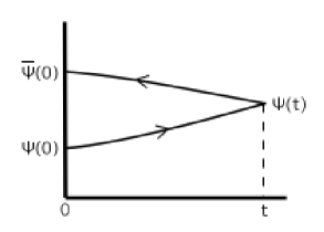
Figure 1: Simple picture for irreversibility.

Here, the state $\bar{\psi}(0)$ is not need to be the same as the original state $\psi(0)$ , that is,

$$\bar{\psi}(0)=\bar{U}\hat{U}\psi(0)$$ (5)

When the Hamiltonian of system is $\hat{H}$, and that of the time reversal world is $\bar{H}$, evolution oparators for each are

$$\hat{U}=\exp\left\{-\frac{i}{\hbar}\hat{H}t\right\}\ ,\ \bar{U}=\exp\left\{+\frac{i}{\hbar}\bar{H}t\right\}$$ (6)

Then, using the Baker-Campbell-Hausdorff formula,

$$\bar{U}\hat{U}=\exp\left\{-\frac{i}{\hbar}(\hat{H}-\bar{H})t+\frac{1}{2\hbar^{2}}[\bar{H},\hat{H}]t^{2}+O(t^{3})+\cdots\right\}$$ (7)

Therefore, the sufficient condition for being ($\bar{U}\hat{U}=1$) or reversible system is being ($\hat{H}=\bar{H}$) .

While, the complex conjugate of eq.(3) and eq.(6)

$$\psi^{*}(t)=\hat{U}^{\dagger}\psi^{*}(0)\quad,\quad\hat{U}^{\dagger}=\exp\left\{+\frac{i}{\hbar}\hat{H}^{\dagger}t\right\}$$ (8)

Then

$$\hat{U}^{\dagger}\hat{U}=\exp\left\{-\frac{i}{\hbar}(\hat{H}-\hat{H}^{\dagger})t+\frac{1}{2\hbar^{2}}[\hat{H}^{\dagger},\hat{H}]t^{2}+O(t^{3})+\cdots\right\}$$ (9)

Therefore the sufficient condition for ($\hat{U}^{\dagger}\hat{U}=1$) or unitary, is that the Hamiltonian is Hermitian, ($\hat{H}^{\dagger}=\hat{H}$).

Now we want to know the relationships between the irreversibility (the break down of time reversal symmetry) and the disappearance of unitarity (the quantum decoherence). Let us show the list of two discussions above.

$$\left.\begin{array}[]{lcl}\bar{H}=\hat{H}\ \mbox{(time reversal symmetry)}&\Rightarrow&\bar{U}\hat{U}=1\ \mbox{(reversibility)}\\ \hat{H}^{\dagger}=\hat{H}\ \mbox{(Hermitian)}&\Rightarrow&\hat{U}^{\dagger}\hat{U}=1\ \mbox{(unitarity)}\end{array}\right\}_{\cap}\Rightarrow\bar{U}=\hat{U}^{\dagger}$$ (10)

It seems that there is no relation between the reversibility and the unitarity from this list.

The lower proposition of eq.(10) is rewritten as follows.

$$\{\hat{U}^{\dagger}\hat{U}=1\}\supset\{\hat{H}^{\dagger}=\hat{H}\}$$ (11)

Here, $\{\cdots\}$ means the region of each event in Venn diagram. Using the De Morgan’s low, we get

$$\{\hat{U}^{\dagger}\hat{U}\neq 1\}\subset\{\hat{H}^{\dagger}\neq\hat{H}\}$$ (12)

Many theoretical and experimantal studies imply that unitarity is lost in systems in which the time reversal symmetry breaks down.

$$\hat{U}^{\dagger}\hat{U}\neq 1\quad\Rightarrow\quad\bar{H}\neq\hat{H}$$ (13)

that is

$$\{\hat{U}^{\dagger}\hat{U}\neq 1\}\subset\{\bar{H}\neq\hat{H}\}$$ (14)

(This inclusion relation is concerned about possibility of unitary dissipation systems.) This relation can’t be derived from discussions above.

But, If we accept a meaning for Hermitian conjugate as the time reversal conjugate, this difficulty is avoided.

$$\hat{H}^{\dagger}\equiv\bar{H},\quad\hat{U}^{\dagger}\equiv\bar{U}$$ (15)

Probably, the relation between complex conjugate and time reversel conjugate has been implied at some textbooks which I have ever read. For example,

$$\psi(t^{\prime})=\exp\left\{-\frac{i}{\hbar}\hat{H}(t^{\prime}-t)\right\}\psi(t)$$ (16)

Its complex conjugate is

$$\psi^{*}(t^{\prime})=\exp\left\{+\frac{i}{\hbar}\hat{H}^{\dagger}(t^{\prime}-t)\right\}\psi^{*}(t)$$ (17)

While, the time reversal ($t^{\prime}-t\rightarrow t-t^{\prime}$) one is

$$\bar{\psi}(t^{\prime})=\exp\left\{+\frac{i}{\hbar}\bar{H}(t^{\prime}-t)\right\}\bar{\psi}(t)$$ (18)

When $\hat{H}$ is Hermitian and time reversal symmetric, eq.(17) and eq.(18) are very alike, therefore they may be identical each other.

$$\psi^{*}(t^{\prime})=\bar{\psi}(t^{\prime}),\psi^{*}(t)=\bar{\psi}(t)$$ (19)

That is, the complex conjugate of wave functions would mean its time reversal conjugate. When we can accept eq.(15), we may define the wave functions for irreversible systems.

When we accept the relation eq.(15), the empirical formula eq.(13) is easily derived.

$$\hat{U}^{\dagger}\hat{U}=\exp\left\{+\frac{i}{\hbar}\hat{H}^{\dagger}t\right\}\exp\left\{-\frac{i}{\hbar}\hat{H}t\right\}=\exp\left\{+\frac{i}{\hbar}\bar{H}t\right\}\exp\left\{-\frac{i}{\hbar}\hat{H}t\right\}$$ (20)

Then,

$$\bar{H}=\hat{H}\quad\Rightarrow\ \ \ \hat{U}^{\dagger}\hat{U}=1$$ (21)

This means that the sufficient condition for unitarity of system is the time reversal symmetry of Hamiltonian. Taking the contraposition, we get

$$\hat{U}^{\dagger}\hat{U}\neq 1\quad\Rightarrow\ \ \ \bar{H}\neq\hat{H}$$ (22)

, which means that the necessary condition for quantum decoherence is the breaking down of time reversal symmetry of Hamiltonian.

In classical system, it is known that irreversibility appears by coarse graining. Averaging procedures destroy microscopic informations for system. It is said that Ergodicity also appears by coarse graining.

Coarse graining makes the system irreversible, and the irreversibility makes the system non-unitary, therefore the coarse graining must make the non-unitarity. Coarse graining is a kind of Projection procedure into a low resolution world, so we can assume that Projection makes the system irreversible. It is known that the Langevin equation is also derived by the projection method.

Projection is a procedure to extract arbitrary sub system from a original system. When the sub system couples with the other neglected (integrated) degrees of freedom in the original system, the coupling effects would be regarded as “the environmental effects” for the sub system. $\diamondsuit$

3 A simple model: Asymmetric triangular harmonic oscillators in Schrödinger cat states, “Three Schrödinger cats”.

Here, We will use a simple model to discuss a possibility of quantum decoherence in a finite system. That is three bosonic particles tied up each other with three springs which have different frequencies. For this model, we will apply the Caldeira & Leggett’s technique. Our three particle model is a extreme reduction of their “harmonic oscillator plus reservoir” model[1].

Figure 2: 3cats model. 3 particles are tied up with springs. And each state is Schrödinger cat.

The main line is, to transform 1-dimensional three particles tied with different springs into two uncoupled harmonic oscillators and one free particle in normal coordinates. And we will derive a propagator for a total wave function of the total system in normal coordinates, and retranslate it into the original system. Then we will be able to get a propagator for harmonically bound three particle. Next, we will prepare the respective initial wave function for each particle as a pair of Gaussian wave packet (the Schrödinger cat state). The initial state of the total system is a product of those states. It will start to turn into a entangle state of three particles by propagator.

In a closed system, it is difficult to suppose that the interference between the wave functions of the closed system will vanish. But we will pay attention to the particle-1 only and integrate out the degrees of freedom about other two particles, then we will get a reduced density function for particle-1. This procedure corresponds to ignoring the fine informations about other two particles and taking an average. Then, we will observe changes of a pair of Gaussian wave packets of particle-1 and the quantum interference term between them.

3.1 Classical model.

Classically, this model (the asymmetric harmonic three body problem) is soluvable, that is a integrable system. Its Lagrangean is as follows.

$$L=\frac{m}{2}\dot{x_{1}}^{2}+\frac{m}{2}\dot{x_{2}}^{2}+\frac{m}{2}\dot{x_{3}}^{2}-\frac{m}{2}\omega_{12}^{2}(x_{1}-x_{2})^{2}-\frac{m}{2}\omega_{13}^{2}(x_{1}-x_{3})^{2}-\frac{m}{2}\omega_{23}^{2}(x_{2}-x_{3})^{2}$$ (23)

Applying the Euler-Lagrange equation

$$\frac{\partial L}{\partial x_{i}}-\frac{d}{dt}\frac{\partial L}{\partial\dot{x_{i}}}=0$$ (24)

to eq.(23), we can get three equations of motion.

$$\frac{d^{2}}{dt^{2}}\left(\begin{array}[]{c}x_{1}\\ x_{2}\\ x_{3}\end{array}\right)=\left(\begin{array}[]{ccc}-(\omega_{12}^{2}+\omega_{13}^{2})&\omega_{12}^{2}&\omega_{13}^{2}\\ \omega_{12}^{2}&-(\omega_{12}^{2}+\omega_{23}^{2})&\omega_{23}^{2}\\ \omega_{13}^{2}&\omega_{23}^{2}&-(\omega_{13}^{2}+\omega_{23}^{2})\end{array}\right)\left(\begin{array}[]{c}x_{1}\\ x_{2}\\ x_{3}\end{array}\right)$$ (25)

Rewriting this,

$$\frac{d^{2}}{dt^{2}}\mbox{\boldmath$X$}_{(t)}=\mbox{\boldmath$W$}\mbox{\boldmath$X$}_{(t)}$$ (26)

and using a time-independent matrix $P$ , then,

$$\frac{d^{2}}{dt^{2}}(\mbox{\boldmath$P$}\mbox{\boldmath$X$}_{(t)})=\mbox{\boldmath$P$}\mbox{\boldmath$W$}\mbox{\boldmath$P$}^{-1}(\mbox{\boldmath$P$}\mbox{\boldmath$X$}_{(t)})$$ (27)

Here, we can set $P$ in order that $\mbox{\boldmath$P$}\mbox{\boldmath$W$}\mbox{\boldmath$P$}^{-1}$ is diagonal, and get three uncoupled differential equations. We will show this procedure. Eigen values of $W$, $\lambda$ satisfy the equation

$$-\left\{\ \lambda^{3}+2(\omega_{12}^{2}+\omega_{13}^{2}+\omega_{23}^{2})\lambda^{2}+3(\omega_{12}^{2}\omega_{13}^{2}+\omega_{13}^{2}\omega_{23}^{2}+\omega_{12}^{2}\omega_{23}^{2})\lambda\ \right\}\equiv 0$$ (28)

We call its 3 solutions $\lambda_{1},\lambda_{2},\lambda_{3}$, and obviously 0 is one solution, then we set it $\lambda_{3}$. And we define

$$\mbox{\boldmath$P$}\mbox{\boldmath$W$}\mbox{\boldmath$P$}^{-1}=\left(\begin{array}[]{ccc}\lambda_{1}&&\\ &\lambda_{2}&\\ &&\lambda_{3}\end{array}\right)=\left(\begin{array}[]{ccc}\lambda_{1}&0&0\\ 0&\lambda_{2}&0\\ 0&0&0\end{array}\right)\equiv\mbox{\boldmath$\Lambda$}$$ (29)

$$\mbox{\boldmath$P$}\mbox{\boldmath$X$}_{(t)}\equiv\mbox{\boldmath$Z$}_{(t)}$$ (30)

Then, equation (27) comes to

$$\frac{d^{2}}{dt^{2}}\mbox{\boldmath$Z$}_{(t)}=\mbox{\boldmath$\Lambda$}\mbox{\boldmath$Z$}_{(t)}$$ (31)

, that is, we can get three independent differential equations as follows.

$$\frac{d^{2}}{dt^{2}}\left(\begin{array}[]{c}z_{1}\\ z_{2}\\ z_{3}\end{array}\right)=\left(\begin{array}[]{ccc}\lambda_{1}&&\\ &\lambda_{2}&\\ &&0\end{array}\right)\left(\begin{array}[]{c}z_{1}\\ z_{2}\\ z_{3}\end{array}\right)=\left(\begin{array}[]{c}\lambda_{1}z_{1}\\ \lambda_{2}z_{2}\\ 0\end{array}\right)$$ (32)

Here we define

$${\mit\Delta}\omega^{2} \equiv \sqrt{\omega_{12}^{4}-\omega_{12}^{2}\omega_{13}^{2}+\omega_{13}^{4}-\omega_{13}^{2}\omega_{23}^{2}+\omega_{23}^{4}-\omega_{23}^{2}\omega_{12}^{2}}$$ (33)

$$= \sqrt{\frac{1}{2}\left\{(\omega_{12}^{2}-\omega_{13}^{2})^{2}+(\omega_{13}^{2}-\omega_{23}^{2})^{2}+(\omega_{23}^{2}-\omega_{12}^{2})^{2}\right\}}$$

$$= \sqrt{(\omega_{12}^{2}+\omega_{13}^{2}+\omega_{23}^{2})^{2}-3\omega_{12}^{2}\omega_{13}^{2}-3\omega_{13}^{2}\omega_{23}^{2}-3\omega_{23}^{2}\omega_{12}^{2}}$$

and from equation (28), $\lambda_{1},\lambda_{2}$ are

$$\left\{\begin{array}[]{l}\lambda_{1}=-\omega_{12}^{2}-\omega_{13}^{2}-\omega_{23}^{2}+{\mit\Delta}\omega^{2}<0\\ \lambda_{2}=-\omega_{12}^{2}-\omega_{13}^{2}-\omega_{23}^{2}-{\mit\Delta}\omega^{2}<0\end{array}\right.$$ (34)

Taking care of their signs, we can solve the equation (32) then we get

$$z_{1(t)}=A_{1}\sin{\Omega_{1}t}+B_{1}\cos{\Omega_{1}t}\quad$$

$$z_{2(t)}=A_{2}\sin{\Omega_{2}t}+B_{2}\cos{\Omega_{2}t}\quad$$

$$z_{3(t)}=C_{1}t+C_{2}\quad$$ (35)

, where

$$\Omega_{1}\equiv\sqrt{-\lambda_{1}},\ \Omega_{2}\equiv\sqrt{-\lambda_{2}}$$ (36)

and $A_{1},A_{2},B_{1},B_{2},C_{1},C_{2}$ are integral constants. They depend on the initial condition of $X$ and $\dot{\mbox{\boldmath$X$}}$. The classical orbit $\mbox{\boldmath$X$}(t)$ is

$$\mbox{\boldmath$X$}_{(t)}=\mbox{\boldmath$P$}^{-1}\mbox{\boldmath$Z$}_{(t)}$$ (37)

We define $W$’s eigen vector ${\bf p_{1},p_{2},p_{3}}$ corresponding to its eigen value $\lambda_{1},\lambda_{2},0$ as follows.

$$\mbox{\boldmath$P$}^{-1}=\left({\bf p_{1}\ p_{2}\ p_{3}}\right)=\left(\begin{array}[]{ccc}\xi_{1}&\xi_{2}&1\\ \eta_{1}&\eta_{2}&1\\ \zeta_{1}&\zeta_{2}&1\end{array}\right)=\left(\begin{array}[]{ccc}\xi_{1}&\xi_{2}&1\\ \eta_{1}&\eta_{2}&1\\ -\xi_{1}-\eta_{1}&-\xi_{2}-\eta_{2}&1\end{array}\right)$$ (38)

Here we difined

$$\begin{array}[]{ll}\xi_{1}=\omega_{12}^{2}\omega_{23}^{2}-\omega_{13}^{2}(\omega_{13}^{2}-{\mit\Delta}\omega^{2})&\xi_{2}=\omega_{12}^{2}\omega_{23}^{2}-\omega_{13}^{2}(\omega_{13}^{2}+{\mit\Delta}\omega^{2})\\ \eta_{1}=\omega_{12}^{2}\omega_{13}^{2}-\omega_{23}^{2}(\omega_{23}^{2}-{\mit\Delta}\omega^{2})&\eta_{2}=\omega_{12}^{2}\omega_{13}^{2}-\omega_{23}^{2}(\omega_{23}^{2}+{\mit\Delta}\omega^{2})\\ \zeta_{1}=-\xi_{1}-\eta_{1}&\zeta_{2}=-\xi_{2}-\eta_{2}\end{array}$$ (39)

Using formulae above, we can get the classical solution of $X$(t) finally.

$$\mbox{\boldmath$X$}_{(t)}=\left(\begin{array}[]{c}x_{1(t)}\\ x_{2(t)}\\ x_{3(t)}\end{array}\right)=\left(\begin{array}[]{c}\xi_{1}z_{1(t)}+\xi_{2}z_{2(t)}+z_{3(t)}\\ \eta_{1}z_{1(t)}+\eta_{2}z_{2(t)}+z_{3(t)}\\ -(\xi_{1}+\eta_{1})z_{1(t)}-(\xi_{2}+\eta_{2})z_{2(t)}+z_{3(t)}\\ \end{array}\right)$$ (40)

Using

$$\Delta\equiv\eta_{2}\xi_{1}-\eta_{1}\xi_{2}$$ (41)

, you can write $P$

$$\mbox{\boldmath$P$}=\frac{1}{3\Delta}\left(\begin{array}[]{ccc}2\eta_{2}+\xi_{2}&-\eta_{2}-2\xi_{2}&-\eta_{2}+\xi_{2}\\ -2\eta_{1}-\xi_{1}&\eta_{1}+2\xi_{1}&\eta_{1}-\xi_{1}\\ \Delta&\Delta&\Delta\end{array}\right)$$ (42)

From the relation

$$\mbox{\boldmath$Z$}_{(t)}=\mbox{\boldmath$P$}\mbox{\boldmath$X$}_{(t)}$$ (43)

, we can get the formula for transformation to the normal coordinate $\mbox{\boldmath$Z$}(t)$.

$$\mbox{\boldmath$Z$}_{(t)}=\left(\begin{array}[]{c}z_{1(t)}\\ z_{2(t)}\\ z_{3(t)}\end{array}\right)=\frac{1}{3\Delta}\left(\begin{array}[]{c}(2\eta_{2}+\xi_{2})x_{1(t)}+(-\eta_{2}-2\xi_{2})x_{2(t)}+(-\eta_{2}+\xi_{2})x_{3(t)}\\ (-2\eta_{1}-\xi_{1})x_{1(t)}+(\eta_{1}+2\xi_{1})x_{2(t)}+(\eta_{1}-\xi_{1})x_{3(t)}\\ \Delta x_{1(t)}+\Delta x_{2(t)}+\Delta x_{3(t)}\\ \end{array}\right)$$ (44)

These formurae are very useful for evaluation of path integrals later.

3.2 Derivation of a propagator

In this section, we derive the Feynman propagator for this 3 body model. It describes evolution of wave functions without differential operators. It is difficult to derive the propagator in the original coordinates $X$, therefore we transform the Lagrangean in the original coordinates into the Lagrangean in the normal coordinates $Z$, where there are two uncoupled harmonic oscillators and a free particle. Its transformation formulae are given in eq.(40) and eq.(44). We substitute them for the original Lagrangean eq.(23), then we get

$$L=\frac{m_{1}}{2}\dot{z}^{2}_{1(t)}+\frac{m_{2}}{2}\dot{z}^{2}_{2(t)}+\frac{m_{3}}{2}\dot{z}^{2}_{3(t)}-\frac{m_{1}}{2}\omega_{1}^{2}z^{2}_{1(t)}-\frac{m_{2}}{2}\omega_{2}^{2}z^{2}_{2(t)}$$ (45)

where

$$m_{1}\equiv 2m(\xi_{1}^{2}+\xi_{1}\eta_{1}+\eta_{1}^{2}),\quad m_{2}\equiv 2m(\xi_{2}^{2}+\xi_{2}\eta_{2}+\eta_{2}^{2}),\quad m_{3}\equiv 3m$$ (46)

$$\left\{\begin{array}[]{c}\omega_{1}^{2}\equiv\frac{m}{m_{1}}\{\ w_{1}^{2}(2\xi_{1}^{2}-\xi_{1}\eta_{1}-\eta_{1}^{2})+w_{2}^{2}(-\xi_{1}^{2}-\xi_{1}\eta_{1}+2\eta_{1}^{2})+w_{3}^{2}(2\xi_{1}^{2}+5\xi_{1}\eta_{1}+2\eta_{1}^{2})\ \}\\ \omega_{2}^{2}\equiv\frac{m}{m_{2}}\{\ w_{1}^{2}(2\xi_{2}^{2}-\xi_{2}\eta_{2}-\eta_{2}^{2})+w_{2}^{2}(-\xi_{2}^{2}-\xi_{2}\eta_{2}+2\eta_{2}^{2})+w_{3}^{2}(2\xi_{2}^{2}+5\xi_{2}\eta_{2}+2\eta_{2}^{2})\ \}\\ (\ w_{1}^{2}=\omega_{12}^{2}+\omega_{13}^{2},\quad w_{2}^{2}=\omega_{12}^{2}+\omega_{23}^{2},\quad w_{3}^{2}=\omega_{13}^{2}+\omega_{23}^{2}\ )\end{array}\right.$$ (47)

, we can decouple the Lagrangean with each variable.

$$L_{1}(z_{1(t)},t)\equiv\frac{m_{1}}{2}\dot{z}^{2}_{1(t)}-\frac{m_{1}}{2}\omega_{1}^{2}z^{2}_{1(t)},\ L_{2}(z_{2(t)},t)\equiv\frac{m_{2}}{2}\dot{z}^{2}_{2(t)}-\frac{m_{2}}{2}\omega_{2}^{2}z^{2}_{2(t)},\$$

$$\quad L_{3}(z_{3(t)},t)\equiv\frac{m_{3}}{2}\dot{z}^{2}_{3(t)}\quad:L=L_{1}+L_{2}+L_{3}$$ (48)

For these Lagrangeans, we can get the classical action integrals summed up from an initial time $t_{0}$ to an arbitrary time $t$.

$$S^{(cl)}(\mbox{\boldmath$Z$}_{(t)},t:\mbox{\boldmath$Z$}_{(t_{0})},t_{0})=\int_{t_{0}}^{t}L_{1(\tau)}d\tau+\int_{t_{0}}^{t}L_{2(\tau)}d\tau+\int_{t_{0}}^{t}L_{3(\tau)}d\tau$$ (49)

$$\quad\quad\equiv S^{(cl)}_{1}(z_{1(t)},t:z_{1(t_{0})},t_{0})+S^{(cl)}_{2}(z_{2(t)},t:z_{2(t_{0})},t_{0})+S^{(cl)}_{3}(z_{3(t)},t:z_{3(t_{0})},t_{0})$$

where

$$S^{(cl)}_{1}=\frac{m_{1}\omega_{1}}{2\sin{\omega_{1}(t-t_{0})}}\left\{\cos{\omega_{1}(t-t_{0})}(z^{2}_{1(t)}+z^{2}_{1(t_{0})})-2z_{1(t)}z_{1(t_{0})}\right\}$$ (50)

$$S^{(cl)}_{2}=\frac{m_{2}\omega_{2}}{2\sin{\omega_{2}(t-t_{0})}}\left\{\cos{\omega_{2}(t-t_{0})}(z^{2}_{2(t)}+z^{2}_{2(t_{0})})-2z_{2(t)}z_{2(t_{0})}\right\}$$ (51)

$$S^{(cl)}_{3}=\frac{m_{3}(z_{3(t)}-z_{3(t_{0})})^{2}}{2(t-t_{0})}$$ (52)

and using these formulae, we get the propagator for wave function in the system $Z$.

$$U(\mbox{\boldmath$Z$},t:\mbox{\boldmath$Z$}_{0},t_{0}) = \int_{\mbox{\boldmath$Z$}(t_{0})=\mbox{\boldmath$Z$}_{0}}^{\mbox{\boldmath$Z$}(t)=\mbox{\boldmath$Z$}}D\mbox{\boldmath$Z$}(\tau)\exp\left\{\frac{i}{\hbar}S(\mbox{\boldmath$Z$},t:\mbox{\boldmath$Z$}(\tau),\tau:\mbox{\boldmath$Z$}_{0},t_{0})\right\}$$ (53)

$$\propto \exp\left\{\frac{i}{\hbar}S^{(cl)}(\mbox{\boldmath$Z$},t:\mbox{\boldmath$Z$}_{0},t_{0})\right\}$$ (54)

Here $D\mbox{\boldmath$Z$}\equiv Dz_{1}Dz_{2}Dz_{3}$ means path integrals about three variables ($z_{1},z_{2},z_{3}$) in system $Z$. The action integral $S(\mbox{\boldmath$Z$},t:\mbox{\boldmath$Z$}(\tau),\tau:\mbox{\boldmath$Z$}_{0},t_{0})$ depends on its integral paths and does not always follow the principle of minimum action. But it is known that the result of path integrals is in proportion to the value of saddle point of their integrands for free particles and for harmonic oscillators, therefore we get equation (54). Its proportional factor depends on the initial time $t_{0}$ and the final time $t$, but here we omit the factor.

Now we assume that the propagator in $Z$ is equivalent to the one in original system $X$, and transform it using equation (40) . Then we get

$$U(\mbox{\boldmath$X$},t:\mbox{\boldmath$X$}_{0},t_{0})=U(\mbox{\boldmath$Z$},t:\mbox{\boldmath$Z$}_{0},t_{0})$$ (55)

$$\qquad\propto\exp\biggl{[}\frac{i}{\hbar}\left\{A_{1}x_{1(0)}^{2}+A_{2}x_{2(0)}^{2}+A_{3}x_{3(0)}^{2}+B_{12}x_{1(0)}x_{2(0)}\right.\biggr{.}$$

$$\qquad\qquad\biggl{.}\left.+B_{23}x_{2(0)}x_{3(0)}+B_{13}x_{1(0)}x_{3(0)}+C_{1}x_{1(0)}+C_{2}x_{2(0)}+C_{3}x_{3(0)}+D\ \right\}\biggr{]}$$

Here using elements of the transformation matrix $P$

$$\begin{array}[]{lll}a_{1}=\frac{1}{3\Delta}(2\eta_{2}+\xi_{2})&a_{2}=\frac{1}{3\Delta}(-\eta_{2}-2\xi_{2})&a_{3}=\frac{1}{3\Delta}(-\eta_{2}+\xi_{2})\\ b_{1}=\frac{1}{3\Delta}(-2\eta_{1}-\xi_{1})&b_{2}=\frac{1}{3\Delta}(\eta_{1}+2\xi_{1})&b_{3}=\frac{1}{3\Delta}(\eta_{1}-\xi_{1})\\ c_{1}=\frac{1}{3}&c_{2}=\frac{1}{3}&c_{3}=\frac{1}{3}\end{array}$$ (56)

($\Delta=\eta_{2}\xi_{1}-\eta_{1}\xi_{2}$), we get the real coefficients in (55) $A_{1}-D$ as follows.

$$A_{i}=\frac{m_{1}\omega_{1}}{2}\cot[\omega_{1}(t-t_{0})]a_{i}^{2}+\frac{m_{2}\omega_{2}}{2}\cot[\omega_{2}(t-t_{0})]b_{i}^{2}+\frac{m_{3}}{2(t-t_{0})}c_{i}^{2}$$ (57)

$$B_{ij}=m_{1}\omega_{1}\cot[\omega_{1}(t-t_{0})]a_{i}a_{j}+m_{2}\omega_{2}\cot[\omega_{2}(t-t_{0})]b_{i}b_{j}+\frac{m_{3}}{(t-t_{0})}c_{i}c_{j}$$

$$C_{i}(\mbox{\boldmath$X$})=-\frac{m_{1}\omega_{1}}{\sin[\omega_{1}(t-t_{0})]}\left(a_{1}x_{1}+a_{2}x_{2}+a_{3}x_{3}\right)a_{i}$$

$$\qquad\qquad\qquad\qquad\qquad-\frac{m_{2}\omega_{2}}{\sin[\omega_{2}(t-t_{0})]}\left(b_{1}x_{1}+b_{2}x_{2}+b_{3}x_{3}\right)b_{i}$$

$$\qquad\qquad\qquad\qquad\qquad\qquad\qquad\qquad-\frac{m_{3}}{(t-t_{0})}\left(c_{1}x_{1}+c_{2}x_{2}+c_{3}x_{3}\right)c_{i}$$

$$D(\mbox{\boldmath$X$})=\frac{m_{1}\omega_{1}}{2}\cot[\omega_{1}(t-t_{0})](a_{1}x_{1}+a_{2}x_{2}+a_{3}x_{3})^{2}$$

$$\qquad\qquad\qquad\qquad\qquad+\frac{m_{2}\omega_{2}}{2}\cot[\omega_{2}(t-t_{0})](b_{1}x_{1}+b_{2}x_{2}+b_{3}x_{3})^{2}$$

$$\qquad\qquad\qquad\qquad\qquad\qquad\qquad\qquad\quad+\frac{m_{3}}{2(t-t_{0})}(c_{1}x_{1}+c_{2}x_{2}+c_{3}x_{3})^{2}$$ (60)

$(i,j=1,2,3)$, and we omitted index $(t)$ , that is $(x_{i(t)}=x_{i})$.

3.3 Derivation of wave function and numerical calculation of reduced density function.

Using this propagator, we can write the development of wave function as follows.

$$\psi(\mbox{\boldmath$X$},t)=\int_{-\infty}^{\infty}d\mbox{\boldmath$X$}_{0}\ U(\mbox{\boldmath$X$},t:\mbox{\boldmath$X$}_{0},t_{0})\ \psi(\mbox{\boldmath$X$}_{0},t_{0})$$ (61)

The initial wave function for our 3 body system is a product of wave functions of each particle at the time $t_{0}$.

$$\psi(\mbox{\boldmath$X$}_{0},t_{0})=\psi_{1}(x_{1(0)},t_{0})\ \psi_{2}(x_{2(0)},t_{0})\ \psi_{3}(x_{3(0)},t_{0})$$ (62)

This means that there has been no interaction among those 3 particles until the initial time $t_{0}$. And the each initial state is the Schrödinger cat state

$$\psi_{1}(x_{1(0)},t_{0})=\tilde{N_{1}}\left[\exp\left\{-\frac{x_{1(0)}^{2}}{4\sigma_{1}^{2}}\right\}+\exp\left\{-\frac{(x_{1(0)}-d_{1})^{2}}{4\sigma_{1}^{2}}\right\}\right]\quad\mbox{etc...}$$ (63)

With equations (55),(62),(63), equation (61) comes to

$$\qquad\ \psi(\mbox{\boldmath$X$},t)\propto\int_{-\infty}^{\infty}dx_{1(0)}\int_{-\infty}^{\infty}dx_{2(0)}\int_{-\infty}^{\infty}dx_{3(0)}$$

$$\times\exp\left[\frac{i}{\hbar}\bigl{\{}A_{1}x_{1(0)}^{2}+A_{2}x_{2(0)}^{2}+A_{3}x_{3(0)}^{2}+B_{12}x_{1(0)}x_{2(0)}+B_{23}x_{2(0)}x_{3(0)}\bigr{.}\right.$$

$$\qquad\qquad\qquad\qquad\qquad\qquad\qquad\biggl{.}\bigl{.}+B_{13}x_{1(0)}x_{3(0)}+C_{1}x_{1(0)}+C_{2}x_{2(0)}+C_{3}x_{3(0)}+D\bigr{\}}\biggr{]}$$

$$\times\biggl{[}\exp\left\{-\frac{x_{1(0)}^{2}}{4\sigma_{1}^{2}}-\frac{x_{2(0)}^{2}}{4\sigma_{2}^{2}}-\frac{x_{3(0)}^{2}}{4\sigma_{3}^{2}}\right\}+\exp\left\{-\frac{(x_{1(0)}-d_{1})^{2}}{4\sigma_{1}^{2}}-\frac{x_{2(0)}^{2}}{4\sigma_{2}^{2}}-\frac{x_{3(0)}^{2}}{4\sigma_{3}^{2}}\right\}+\cdots$$

$$\qquad\qquad\cdots+\exp\left\{-\frac{(x_{1(0)}-d_{1})^{2}}{4\sigma_{1}^{2}}-\frac{(x_{2(0)}-d_{2})^{2}}{4\sigma_{2}^{2}}-\frac{(x_{3(0)}-d_{3})^{2}}{4\sigma_{3}^{2}}\right\}\biggr{]}$$ (64)

The latter $[\cdots]$ of this formula means 8 Gaussian packet in ($x_{1},x_{2},x_{3}$) space. Each packet changes by propagator. For evaluating analytic forms of those packets, integrations with three variables ($x_{1(0)},x_{2(0)},x_{3(0)}$) are needed. With the new complex coefficients $\breve{A}_{1}-\breve{D}$, eq.(64) turns into

$$\qquad\ \psi(\mbox{\boldmath$X$},t)=\sum_{k=0-7}\psi^{(k)}(\mbox{\boldmath$X$},t)$$ (65)

$$\qquad\ \psi^{(k)}(\mbox{\boldmath$X$},t)\propto\int_{-\infty}^{\infty}dx_{1(0)}\int_{-\infty}^{\infty}dx_{2(0)}\int_{-\infty}^{\infty}dx_{3(0)}$$

$$\times\exp\left[-\breve{A}_{1}x_{1(0)}^{2}-\breve{A}_{2}x_{2(0)}^{2}-\breve{A}_{3}x_{3(0)}^{2}+\breve{B}_{12}x_{1(0)}x_{2(0)}+\breve{B}_{23}x_{2(0)}x_{3(0)}\right.$$

$$\qquad\qquad\qquad\qquad\qquad\biggl{.}+\breve{B}_{13}x_{1(0)}x_{3(0)}+\breve{C}^{(k)}_{1}x_{1(0)}+\breve{C}^{(k)}_{2}x_{2(0)}+\breve{C}^{(k)}_{3}x_{3(0)}+\breve{D}^{(k)}\biggr{]}$$

(66)

($k=0-7$), which is the Gaussian integrals we have to solve .

$$\breve{A}_{1}=\frac{1}{4\sigma_{1}^{2}}-\frac{i}{\hbar}A_{1},\quad\breve{B}_{12}=\frac{i}{\hbar}B_{12},\quad\breve{C}^{(k)}_{1}(\mbox{\boldmath$X$})=\frac{d^{(k)}_{1}}{2\sigma_{1}^{2}}+\frac{i}{\hbar}C_{1}(\mbox{\boldmath$X$})\quad\mbox{etc...}$$

$$\qquad\qquad\breve{D}^{(k)}(\mbox{\boldmath$X$})=-\frac{d^{(k)2}_{1}}{4\sigma_{1}^{2}}-\frac{d^{(k)2}_{2}}{4\sigma_{2}^{2}}-\frac{d^{(k)2}_{3}}{4\sigma_{3}^{2}}+\frac{i}{\hbar}D(\mbox{\boldmath$X$})$$ (67)

where

$$\left(\begin{array}[]{rrcccl}&[&d^{(k)}_{1}&d^{(k)}_{2}&d^{(k)}_{3}&]\\ k=0&[&\ 0&\ 0&\ 0&]\\ 1&[&d_{1}&\ 0&\ 0&]\\ 2&[&\ 0&d_{2}&\ 0&]\\ 3&[&\ 0&\ 0&d_{3}&]\end{array}\quad\begin{array}[]{rrcccl}&&&&&\\ 4&[&d_{1}&d_{2}&\ 0&]\\ 5&[&d_{1}&\ 0&d_{3}&]\\ 6&[&\ 0&d_{2}&d_{3}&]\\ 7&[&d_{1}&d_{2}&d_{3}&]\end{array}\right)$$ (68)

Evaluating this Gaussian integrals, we get

$$\psi^{(k)}(\mbox{\boldmath$X$},t)\propto\sqrt{\frac{\pi^{3}}{\Delta}}\exp\left[\frac{1}{16\Delta}\Phi^{(k)}(\mbox{\boldmath$X$},t)+\breve{D}^{(k)}(\mbox{\boldmath$X$},t)\right]$$ (69)

where

$$\Delta(t)=\breve{A}_{1}\breve{A}_{2}\breve{A}_{3}-\frac{1}{4}(\breve{A}_{2}\breve{B}^{2}_{13}+\breve{A}_{3}\breve{B}^{2}_{12}+\breve{A}_{1}\breve{B}^{2}_{23})-\frac{1}{4}\breve{B}_{12}\breve{B}_{13}\breve{B}_{23}$$ (70)

$$\qquad\ \equiv\Re e\Delta(t)+i\ \Im m\Delta(t)$$ (71)

$$\quad\Re e\Delta(t)=\frac{1}{4^{3}\sigma_{1}^{2}\sigma_{2}^{2}\sigma_{3}^{2}}-\frac{1}{4\hbar^{2}}\left(\frac{A_{2}A_{3}}{\sigma_{1}^{2}}+\frac{A_{3}A_{1}}{\sigma_{2}^{2}}+\frac{A_{1}A_{2}}{\sigma_{3}^{2}}\right)$$

$$\qquad\qquad\qquad\qquad+\frac{1}{16\hbar^{2}}\left(\frac{B_{23}^{2}}{\sigma_{1}^{2}}+\frac{B_{13}^{2}}{\sigma_{2}^{2}}+\frac{B_{12}^{2}}{\sigma_{3}^{2}}\right)$$ (72)

$$\quad\Im m\Delta(t)=\frac{1}{\hbar^{3}}A_{1}A_{2}A_{3}-\frac{1}{16\hbar}\left(\frac{A_{3}}{\sigma_{1}^{2}\sigma_{2}^{2}}+\frac{A_{1}}{\sigma_{2}^{2}\sigma_{3}^{2}}+\frac{A_{2}}{\sigma_{3}^{2}\sigma_{1}^{2}}\right)$$

$$\qquad\qquad\qquad\qquad-\frac{1}{4\hbar^{3}}(A_{1}B_{23}^{2}+A_{2}B_{13}^{2}+A_{3}B_{12}^{2})+\frac{1}{4\hbar^{3}}B_{12}B_{13}B_{23}$$ (73)

while

$$\Phi^{(k)}(\mbox{\boldmath$X$},t)=4(\ \breve{A}_{2}\breve{A}_{3}\breve{C}^{2}_{1}(\mbox{\boldmath$X$})+\breve{A}_{1}\breve{A}_{3}\breve{C}^{2}_{2}(\mbox{\boldmath$X$})+\breve{A}_{1}\breve{A}_{2}\breve{C}^{2}_{3}(\mbox{\boldmath$X$})\ )$$

$$\qquad\qquad\qquad-\breve{B}_{23}^{2}\breve{C}_{1}^{2}(\mbox{\boldmath$X$})-\breve{B}_{13}^{2}\breve{C}_{2}^{2}(\mbox{\boldmath$X$})-\breve{B}_{12}^{2}\breve{C}_{3}^{2}(\mbox{\boldmath$X$})$$

$$\qquad+2(\ \breve{B}_{13}\breve{B}_{23}\breve{C}_{1}(\mbox{\boldmath$X$})\breve{C}_{2}(\mbox{\boldmath$X$})+\breve{B}_{12}\breve{B}_{13}\breve{C}_{2}(\mbox{\boldmath$X$})\breve{C}_{3}(\mbox{\boldmath$X$})+\breve{B}_{12}\breve{B}_{23}\breve{C}_{1}(\mbox{\boldmath$X$})\breve{C}_{3}(\mbox{\boldmath$X$})\ )$$

$$\qquad\qquad+4(\ \breve{A}_{1}\breve{B}_{23}\breve{C}_{2}(\mbox{\boldmath$X$})\breve{C}_{3}(\mbox{\boldmath$X$})+\breve{A}_{2}\breve{B}_{13}\breve{C}_{1}(\mbox{\boldmath$X$})\breve{C}_{3}(\mbox{\boldmath$X$})+\breve{A}_{3}\breve{B}_{12}\breve{C}_{1}(\mbox{\boldmath$X$})\breve{C}_{2}(\mbox{\boldmath$X$})\ )$$

(74)

We introduce new complex coefficients

$$(4\breve{A}_{2}\breve{A}_{3}-\breve{B}_{23}^{2})\equiv\lambda_{1}\ \mbox{etc..}\ ,\ (2\breve{B}_{13}\breve{B}_{23}+4\breve{A}_{3}\breve{B}_{12})\equiv\mu_{12}\ \mbox{etc..}$$ (75)

, then we can rewrite $\Phi^{(k)}$ as follows.

$$\Phi^{(k)}(\mbox{\boldmath$X$},t)=\sum_{i=1}^{3}\lambda_{i}\breve{C}_{i}^{2}(\mbox{\boldmath$X$})\ +\ \sum_{\stackrel{{\scriptstyle\scriptstyle(i,j)=(1,2)\mbox{ \small or}}}{{\scriptstyle(2,3)\mbox{ \small or }(3,1)}}}\mu_{ij}\breve{C}_{i}(\mbox{\boldmath$X$})\breve{C}_{j}(\mbox{\boldmath$X$})\qquad\qquad\quad$$ (76)

Here, we write the real part and the imaginary part of $\lambda_{i}$ and $\mu_{ij}$.

$$\lambda_{i}\equiv\Re e\lambda_{i}+i\ \Im m\lambda_{i}$$ (77)

$$\quad\Re e\lambda_{i}=-\frac{1}{\hbar^{2}}\biggl{\{}\ m_{1}\omega_{1}\cot[\omega_{1}(t-t_{0})]\ m_{2}\omega_{2}\cot[\omega_{2}(t-t_{0})]\ (a_{j}b_{k}-a_{k}b_{j})^{2}\biggr{.}$$

$$\qquad\qquad\qquad\qquad\qquad+m_{2}\omega_{2}\cot[\omega_{2}(t-t_{0})]\ \frac{m_{3}}{(t-t_{0})}\ (b_{j}c_{k}-b_{k}c_{j})^{2}$$

$$\qquad\qquad\qquad\qquad\biggl{.}+\frac{m_{3}}{(t-t_{0})}\ m_{1}\omega_{1}\cot[\omega_{1}(t-t_{0})]\ (c_{j}a_{k}-c_{k}a_{j})^{2}\ \biggr{\}}+\frac{1}{4\sigma_{j}^{2}\sigma_{k}^{2}}$$ (78)

$$\quad\Im m\lambda_{i}=-\frac{1}{2\hbar}\biggl{\{}\ m_{1}\omega_{1}\cot[\omega_{1}(t-t_{0})]\left(\frac{a_{j}^{2}}{\sigma_{k}^{2}}+\frac{a_{k}^{2}}{\sigma_{j}^{2}}\right)$$

$$\qquad\qquad\qquad\qquad\quad+m_{2}\omega_{2}\cot[\omega_{2}(t-t_{0})]\left(\frac{b_{j}^{2}}{\sigma_{k}^{2}}+\frac{b_{k}^{2}}{\sigma_{j}^{2}}\right)+\frac{m_{3}}{(t-t_{0})}\left(\frac{c_{j}^{2}}{\sigma_{k}^{2}}+\frac{c_{k}^{2}}{\sigma_{j}^{2}}\right)\ \biggr{\}}$$

(79)

and

$$\mu_{ij}\equiv\Re e\mu_{ij}+i\ \Im m\mu_{ij}$$ (80)

$$\ \Re e\mu_{ij}=-\frac{2}{\hbar^{2}}\biggl{\{}m_{1}\omega_{1}\cot[\omega_{1}(t-t_{0})]\ m_{2}\omega_{2}\cot[\omega_{2}(t-t_{0})]\ (a_{j}b_{k}-a_{k}b_{j})(a_{k}b_{i}-a_{i}b_{k})\biggr{.}$$

$$\qquad\qquad\qquad\qquad\ +m_{2}\omega_{2}\cot[\omega_{2}(t-t_{0})]\ \frac{m_{3}}{(t-t_{0})}\ (b_{j}c_{k}-b_{k}c_{j})(b_{k}c_{i}-b_{i}c_{k})$$

$$\qquad\qquad\qquad\qquad\quad\ \biggl{.}+\frac{m_{3}}{(t-t_{0})}\ m_{1}\omega_{1}\cot[\omega_{1}(t-t_{0})]\ (c_{j}a_{k}-c_{k}a_{j})(c_{k}a_{i}-c_{i}a_{k})\ \biggr{\}}$$

(81)

$$\ \Im m\mu_{ij}=\frac{1}{\sigma_{k}^{2}\hbar}\biggl{\{}m_{1}\omega_{1}\cot[\omega_{1}(t-t_{0})]a_{i}a_{j}\biggr{.}$$

$$\qquad\qquad\qquad\qquad\qquad\qquad\qquad\quad\ \biggl{.}+m_{2}\omega_{2}\cot[\omega_{2}(t-t_{0})]b_{i}b_{j}\ +\frac{m_{3}}{(t-t_{0})}c_{i}c_{j}\ \biggr{\}}$$

(82)

$$\qquad\qquad\qquad\qquad\bigl{(}\ (i,j,k)=(1,2,3)\ \mbox{or}\ (2,3,1)\ \mbox{or}\ (3,1,2)\ \bigr{)}$$

And we introduce new complex factors ($La_{11}-Mu^{(k)}_{0}$).

$$\quad La_{dd}=\sum_{i=1}^{3}\lambda_{i}\alpha_{d}^{(i)2},\quad Mu_{dd}=\sum_{\stackrel{{\scriptstyle\scriptstyle(i,j)=(1,2)\mbox{ \small or}}}{{\scriptstyle(2,3)\mbox{ \small or }(3,1)}}}\mu_{ij}\alpha_{d}^{(i)}\alpha_{d}^{(j)}\quad(\ d=1,2,3\ )$$ (83)

$$La_{df}=2\sum_{i=1}^{3}\lambda_{i}\alpha_{d}^{(i)}\alpha_{f}^{(i)},\quad Mu_{df}=\sum_{(i,j)}\mu_{ij}\left(\alpha_{d}^{(i)}\alpha_{f}^{(j)}+\alpha_{d}^{(j)}\alpha_{f}^{(i)}\right)$$ (84)

$$\qquad\qquad\qquad\bigl{(}\ (d,f)=(1,2)\ \mbox{or}\ (2,3)\ \mbox{or}\ (3,1)\ \bigr{)}$$

$$La_{d}^{(k)}=\sum_{i=1}^{3}\lambda_{i}\frac{d_{i}^{(k)}}{\sigma_{i}^{2}}\alpha_{d}^{(i)},\quad Mu_{d}^{(k)}=0.5\sum_{(i,j)}\mu_{ij}\left(\frac{d_{i}^{(k)}}{\sigma_{i}^{2}}\alpha_{d}^{(j)}+\frac{d_{j}^{(k)}}{\sigma_{j}^{2}}\alpha_{d}^{(i)}\right)$$ (85)

$$\quad La_{0}^{(k)}=0.25\sum_{i=1}^{3}\lambda_{i}\frac{d_{i}^{(k)2}}{\sigma_{i}^{4}},\quad Mu_{0}^{(k)}=0.25\sum_{(i,j)}\mu_{ij}\frac{d_{i}^{(k)}}{\sigma_{i}^{2}}\frac{d_{j}^{(k)}}{\sigma_{j}^{2}}$$ (86)

this $\alpha_{d}^{(i)}$ are real,

$$\quad C_{i}(\mbox{\boldmath$X$})=-\alpha_{1}^{(i)}x_{1}-\alpha_{2}^{(i)}x_{2}-\alpha_{3}^{(i)}x_{3}$$ (87)

$$\alpha_{d}^{(i)}\equiv\left(\frac{m_{1}\omega_{1}}{\sin[\omega_{1}(t-t_{0})]}a_{i}\right)a_{d}+\left(\frac{m_{2}\omega_{2}}{\sin[\omega_{2}(t-t_{0})]}b_{i}\right)b_{d}+\left(\frac{m_{3}}{(t-t_{0})}c_{i}\right)c_{d}$$

(88)

therefore the real and the imaginary part of ( $La_{11}-Mu^{(k)}_{0}$ ) simply correspond to the real part and the imaginary part of ( $\lambda_{i},\mu_{ij}$ ) respectively, that is

$$\quad\Re eLa_{dd}=\sum_{i=1}^{3}\Re e\lambda_{i}\alpha_{d}^{(i)2}\quad\mbox{etc..}$$ (89)

Then the real and the imaginary part of $\Phi^{(k)}$ are

$$\Phi^{(k)}(\mbox{\boldmath$X$},t)\equiv\Re e\Phi^{(k)}(\mbox{\boldmath$X$},t)+i\ \Im m\Phi^{(k)}(\mbox{\boldmath$X$},t)$$ (90)

With the help of the formulae above,

$$\quad\Re e\Phi^{(k)}(\mbox{\boldmath$X$},t)=-\frac{1}{\hbar^{2}}(\Re eLa_{11}+\Re eMu_{11})x_{1}^{2}-\frac{1}{\hbar^{2}}(\Re eLa_{22}+\Re eMu_{22})x_{2}^{2}$$

$$\qquad\qquad\qquad\qquad\ -\frac{1}{\hbar^{2}}(\Re eLa_{33}+\Re eMu_{33})x_{3}^{2}-\frac{1}{\hbar^{2}}(\Re eLa_{12}+\Re eMu_{12})x_{1}x_{2}$$

$$\qquad\qquad\qquad\qquad-\frac{1}{\hbar^{2}}(\Re eLa_{23}+\Re eMu_{23})x_{2}x_{3}-\frac{1}{\hbar^{2}}(\Re eLa_{31}+\Re eMu_{31})x_{3}x_{1}$$

$$\qquad\qquad\qquad\qquad\ +\frac{1}{\hbar}(\Im mLa^{(k)}_{1}+\Im mMu^{(k)}_{1})x_{1}+\frac{1}{\hbar}(\Im mLa^{(k)}_{2}+\Im mMu^{(k)}_{2})x_{2}$$

$$\qquad\qquad\qquad\qquad\quad+\frac{1}{\hbar}(\Im mLa^{(k)}_{3}+\Im mMu^{(k)}_{3})x_{3}+\Re eLa^{(k)}_{0}+\Re eMu^{(k)}_{0}$$ (91)

$$\quad\Im m\Phi^{(k)}(\mbox{\boldmath$X$},t)=-\frac{1}{\hbar^{2}}(\Im mLa_{11}+\Im mMu_{11})x_{1}^{2}-\frac{1}{\hbar^{2}}(\Im mLa_{22}+\Im mMu_{22})x_{2}^{2}$$

$$\qquad\qquad\qquad\qquad\ \ -\frac{1}{\hbar^{2}}(\Im mLa_{33}+\Im mMu_{33})x_{3}^{2}-\frac{1}{\hbar^{2}}(\Im mLa_{12}+\Im mMu_{12})x_{1}x_{2}$$

$$\qquad\qquad\qquad\qquad-\frac{1}{\hbar^{2}}(\Im mLa_{23}+\Im mMu_{23})x_{2}x_{3}-\frac{1}{\hbar^{2}}(\Im mLa_{31}+\Im mMu_{31})x_{3}x_{1}$$

$$\qquad\qquad\qquad\qquad\ -\frac{1}{\hbar}(\Re eLa^{(k)}_{1}+\Re eMu^{(k)}_{1})x_{1}-\frac{1}{\hbar}(\Re eLa^{(k)}_{2}+\Re eMu^{(k)}_{2})x_{2}$$

$$\qquad\qquad\qquad\qquad\quad-\frac{1}{\hbar}(\Re eLa^{(k)}_{3}+\Re eMu^{(k)}_{3})x_{3}+\Im mLa^{(k)}_{0}+\Im mMu^{(k)}_{0}$$ (92)

And another formula $\breve{D}^{(k)}(\mbox{\boldmath$X$})$ is

$$\breve{D}^{(k)}(\mbox{\boldmath$X$})\equiv\Re e\breve{D}^{(k)}+i\ \Im m\breve{D}(\mbox{\boldmath$X$})$$ (93)

$$\qquad\Re e\breve{D}^{(k)}=-\frac{d_{1}^{(k)2}}{4\sigma_{1}^{2}}-\frac{d_{2}^{(k)2}}{4\sigma_{2}^{2}}-\frac{d_{3}^{(k)2}}{4\sigma_{3}^{2}}$$ (94)

$$\qquad\Im m\breve{D}(\mbox{\boldmath$X$})=D(\mbox{\boldmath$X$})/\hbar$$ (95)

Next, the wave function is from eq.(69),

$$\psi^{(k)}(\mbox{\boldmath$X$},t)\propto\sqrt{\frac{\pi^{3}\Delta^{*}}{|\Delta|^{2}}}\ \exp\left[\ \frac{\Delta^{*}}{16|\Delta|^{2}}\Phi^{(k)}(\mbox{\boldmath$X$},t)+\breve{D}^{(k)}(\mbox{\boldmath$X$},t)\ \right]$$ (96)

$$\qquad\qquad\quad\equiv\ \breve{Q}\ \exp[\ \Theta^{(k)}(\mbox{\boldmath$X$},t)\ ]$$ (97)

where

$$\qquad\qquad\qquad\qquad\qquad\breve{Q}\equiv\Re e\breve{Q}+i\ \Im m\breve{Q}$$ (98)

$$\Re e\breve{Q}=\sqrt{\frac{\pi^{3}}{|\Delta|}}\ \cos\frac{\phi}{2}\ ,\quad\Im m\breve{Q}=\sqrt{\frac{\pi^{3}}{|\Delta|}}\ \sin\frac{\phi}{2}\ \quad:\phi=\arctan\left(\Im m\Delta/\Re e\Delta\right)$$

(99)

and

$$\qquad\qquad\qquad\Theta^{(k)}(\mbox{\boldmath$X$},t)\equiv\Re e\Theta^{(k)}(\mbox{\boldmath$X$},t)+i\ \Im m\Theta^{(k)}(\mbox{\boldmath$X$},t)$$ (100)

$$\Re e\Theta^{(k)}(\mbox{\boldmath$X$},t)=\frac{1}{16|\Delta|^{2}}(\ \Re e\Delta\cdot\Re e\Phi^{(k)}+\Im m\Delta\cdot\Im m\Phi^{(k)}\ )+\Re e\breve{D}^{(k)}$$ (101)

$$\Im m\Theta^{(k)}(\mbox{\boldmath$X$},t)=\frac{1}{16|\Delta|^{2}}(\ \Re e\Delta\cdot\Im m\Phi^{(k)}-\Im m\Delta\cdot\Re e\Phi^{(k)}\ )+\Im m\breve{D}(\mbox{\boldmath$X$})$$ (102)

Then, the real part and the imaginary part of the wave function are as follows.

$$\quad\qquad\quad\ \psi^{(k)}(\mbox{\boldmath$X$},t)\equiv\Re e\psi^{(k)}(\mbox{\boldmath$X$},t)+i\ \Im m\psi^{(k)}(\mbox{\boldmath$X$},t)$$ (103)

$$\Re e\psi^{(k)}(\mbox{\boldmath$X$},t)\propto\exp[\ \Re e\Theta^{(k)}\ ]\left(\ \Re e\breve{Q}\cdot\cos[\Im m\Theta^{(k)}]-\Im m\breve{Q}\cdot\sin[\Im m\Theta^{(k)}]\ \right)$$

$$\qquad\qquad\qquad=\sqrt{\frac{\pi^{3}}{|\Delta|}}\ \exp[\ \Re e\Theta^{(k)}\ ]\cdot\cos\left[\ \Im m\Theta^{(k)}+\frac{\phi}{2}\ \right]$$ (104)

$$\Im m\psi^{(k)}(\mbox{\boldmath$X$},t)\propto\exp[\ \Re e\Theta^{(k)}\ ]\left(\ \Re e\breve{Q}\cdot\sin[\Im m\Theta^{(k)}]+\Im m\breve{Q}\cdot\cos[\Im m\Theta^{(k)}]\ \right)$$

$$\qquad\qquad\qquad=\sqrt{\frac{\pi^{3}}{|\Delta|}}\ \exp[\ \Re e\Theta^{(k)}\ ]\cdot\sin\left[\ \Im m\Theta^{(k)}+\frac{\phi}{2}\ \right]$$ (105)

Therefore the total wave function summed with ($k=0-7$) is

$$\psi^{(total)}(\mbox{\boldmath$X$},t)\equiv\Re e\psi^{(total)}(\mbox{\boldmath$X$},t)+i\ \Im m\psi^{(total)}(\mbox{\boldmath$X$},t)$$ (106)

$$\qquad\Re e\psi^{(total)}=C\sqrt{\frac{\pi^{3}}{|\Delta|}}\ \sum_{k=0}^{7}\exp[\ \Re e\Theta^{(k)}\ ]\cdot\cos\left[\ \Im m\Theta^{(k)}+\frac{\phi}{2}\ \right]$$ (107)

$$\qquad\Im m\psi^{(total)}=C\sqrt{\frac{\pi^{3}}{|\Delta|}}\ \sum_{k=0}^{7}\exp[\ \Re e\Theta^{(k)}\ ]\cdot\sin\left[\ \Im m\Theta^{(k)}+\frac{\phi}{2}\ \right]$$ (108)

Here we introduced a real normalization constant $C$. Then the quantum mechanical probability density function of total system become as follows.

$$\rho^{(total)}(\mbox{\boldmath$X$},t)=\Re e^{2}\psi^{(total)}+\Im m^{2}\psi^{(total)}$$

$$\qquad=C^{2}\frac{\pi^{3}}{|\Delta|}\ \sum_{k=0}^{7}\sum_{l=0}^{7}\exp[\ \Re e\Theta^{(k)}+\Re e\Theta^{(l)}\ ]\cdot\cos[\ \Im m\Theta^{(k)}-\Im m\Theta^{(l)}\ ]$$

$$\qquad=C^{2}\frac{\pi^{3}}{|\Delta|}\biggl{(}\sum_{k=0}^{7}\exp[\ 2\Re e\Theta^{(k)}\ ]$$

$$\qquad\qquad\qquad\qquad+2\sum_{k<l}^{0-7}\exp[\ \Re e\Theta^{(k)}+\Re e\Theta^{(l)}\ ]\cdot\cos[\ \Im m\Theta^{(k)}-\Im m\Theta^{(l)}\ ]\biggr{)}$$

The first term in $(\cdots)$ of equation (3.3) means the eight wave packets which originally are the Gaussian packets at the initial time ($t=t_{0}$). While the second term is their “interference” term, which is not the same as the quantum interference vanishes by quantum decoherence in this model.

Note that we are not interested in informations about total 3-body system, we are interested in only the information about particle-1 as a sub-system. Therefore we should integrate out informations about particle-2 and -3. Then we can get the information about particle-1 only, that is, the reduced density function for particle-1.

$$\tilde{\rho}_{1}^{(reduced)}(x_{1},t)\equiv\int_{-\infty}^{\infty}\int_{-\infty}^{\infty}dx_{2}\ dx_{3}\ \rho^{(total)}(\mbox{\boldmath$X$},t)$$ (110)

We substitute eq.(3.3) into eq.(110),

$$\tilde{\rho}_{1}^{(reduced)}(x_{1},t)=C^{2}\frac{\pi^{3}}{|\Delta|}\biggl{(}\sum_{k=0}^{7}\int_{-\infty}^{\infty}\int_{-\infty}^{\infty}dx_{2}\ dx_{3}\ \exp[\ 2\Re e\Theta^{(k)}\ ]$$

$$\qquad+2\sum_{k<l}^{0-7}\int_{-\infty}^{\infty}\int_{-\infty}^{\infty}dx_{2}\ dx_{3}\ \exp[\ \Re e\Theta^{(k)}+\Re e\Theta^{(l)}\ ]\cdot\cos[\ \Im m\Theta^{(k)}-\Im m\Theta^{(l)}\ ]\biggr{)}$$

(111)

Here we notice that there are two kinds of “interference term”. When there is a interference between different packets, macroscopic states of particle-1 included in each packet may be the same. It is simple that we think the initial states. From eq.(68),

$$\begin{array}[]{cl}k=0,2,3,6&\mbox{: \ The packet around ($x_{1}=0$) at initial time ($t=t_{0}$).}\\ k=1,4,5,7&\mbox{: \ The packet around ($x_{1}=d_{1}$) at initial time. }\end{array}$$ (112)

The 8 packets in the ($x_{1},x_{2},x_{3}$) space are separated into these two groups. The interference between packets in the same group means the transition between the states for particle-2 and 3, not for particle-1. Because the particle-1 is in the same its own state, these are not the true interferences between different states for particle-1 which really we want to see.

Now we have to separate these 8 packets into two groups above, and we have to add the “interference” terms among the packets in the same group to the packet terms. We regard them as the effective states for the particle-1. That is,
$\bigcirc$ The packet around ($x_{1}=0$) at initial time $t_{0}$.

$$\tilde{\rho}_{1\_0}^{\mbox{ \tiny eff}}(x_{1},t)\equiv C^{2}\frac{\pi^{3}}{|\Delta|}\sum_{k=0,2,3,6}\biggl{(}\int_{-\infty}^{\infty}\int_{-\infty}^{\infty}dx_{2}\ dx_{3}\ \exp[\ 2\Re e\Theta^{(k)}\ ]$$

$$\quad+2\sum_{l=0,2,3,6}^{k<l}\int_{-\infty}^{\infty}\int_{-\infty}^{\infty}dx_{2}\ dx_{3}\ \exp[\ \Re e\Theta^{(k)}+\Re e\Theta^{(l)}\ ]\cdot\cos[\ \Im m\Theta^{(k)}-\Im m\Theta^{(l)}\ ]\biggr{)}$$

(113)

$\bigcirc$ The packet around ($x_{1}=d_{1}$) at initial time $t_{0}$.

$$\tilde{\rho}_{1\_d}^{\mbox{ \tiny eff}}(x_{1},t)\equiv C^{2}\frac{\pi^{3}}{|\Delta|}\sum_{k=1,4,5,7}\biggl{(}\int_{-\infty}^{\infty}\int_{-\infty}^{\infty}dx_{2}\ dx_{3}\ \exp[\ 2\Re e\Theta^{(k)}\ ]$$

$$\quad+2\sum_{l=1,4,5,7}^{k<l}\int_{-\infty}^{\infty}\int_{-\infty}^{\infty}dx_{2}\ dx_{3}\ \exp[\ \Re e\Theta^{(k)}+\Re e\Theta^{(l)}\ ]\cdot\cos[\ \Im m\Theta^{(k)}-\Im m\Theta^{(l)}\ ]\biggr{)}$$

(114)

$\bigcirc$ Their interference term.

$$\tilde{\rho}_{1\_int}^{\mbox{ \tiny eff}}(x_{1},t)\equiv 4C^{2}\frac{\pi^{3}}{|\Delta|}\sum_{\stackrel{{\scriptstyle\scriptstyle k=0,2,3,6}}{{\scriptstyle l=1,4,5,7}}}^{k<l}\int_{-\infty}^{\infty}\int_{-\infty}^{\infty}dx_{2}\ dx_{3}\ \exp[\ \Re e\Theta^{(k)}+\Re e\Theta^{(l)}\ ]\cdot\cos[\ \Im m\Theta^{(k)}-\Im m\Theta^{(l)}\ ]$$ (115)

Finally, we get the reduced density for particle-1 as follows.

$$\tilde{\rho}_{1}(x_{1},t)=\tilde{\rho}_{1\_0}^{\mbox{ \tiny eff}}(x_{1},t)+\tilde{\rho}_{1\_d}^{\mbox{ \tiny eff}}(x_{1},t)+\tilde{\rho}_{1\_int}^{\mbox{ \tiny eff}}(x_{1},t)$$ (116)

We used numerical calculation for integrations in eq.(110) and final normalization.

3.4 Simulation Result

The case $\omega_{12}=0.305$, $\omega_{13}=0.1$, $\omega_{23}=0.202$ is showed as follows. From upper left to bottom right, the figures are corresponding to time
$t=0.005,\ 0.705,\ 1.405,\ 2.105,\ 2.805,\ 4.205,\ 5.605,\ 205.605,\ 2000.005,\ 5000.005$
, respectively. As you can see, there are 2 packets in each figure. The right packet is [$\tilde{\rho}_{1\_0}^{\mbox{ \tiny eff}}$] which is in the origin ($x_{1}=0$) initially. The left packet is [$\tilde{\rho}_{1\_d}^{\mbox{ \tiny eff}}$] which is in ($x_{1}=d_{1}$) initially. And there are 2 wave-like lines. The lower wave line is the quantum interference term [$\tilde{\rho}_{1\_int}^{\mbox{ \tiny eff}}$] between these 2 packets, whose disappearance means the emergence of classicality. The upper wave line is their total reduced density for particle 1, [$\tilde{\rho}_{1}(x_{1},t)$]. Their horizontal axes are particle-1’s position, $x_{1}$.

Figure 3: $\Uparrow$ (Left) t=0.005, (Right) t=0.705

Figure 4: $\Uparrow$ (Left) t=1.405, (Right) t=2.105

Figure 5: $\Uparrow$ (Left) t=2.805, (Right) t=4.205

Figure 6: $\Uparrow$ (Left) t=5.605, (Right) t=205.605

Figure 7: $\Uparrow$ (Left) t=2000.005, (Right) t=5000.005

In this case, momentarily the interference between two packets are strong, but after the time t $\simeq$ 5.6, the interferences are comparatively weakened. It means the quantum decoherence arises.

By this Three Schrödinger cats model, it was showed that the quantum decoherence would arise in a 1-body sub-system of a closed finite system which consists of three degrees of freedom. In other words, it was showed that decoherence would arise in an opened 1-body system with only two envoronmental degrees of freedom. $\diamondsuit$

4 Discussion

We showed the possibility of emergence of classicality in a quantum mechanical system with 3 degrees of freedom. What did make this quantum decoherence? In this model, we selected only 1 degree as main system, and regarded other 2 degrees of freedom as environments. Then, the quantum mechanical property of the main system vanished because of the “environmental effects” of other two degrees of freedom. They disturbed the main system and destroyed its quantum interference.

For decoherence, it seems that “randomness” is important. It is known that external random forces make a system decoherence. But remember that the introduction of “randomness” is only an artificial procedure. If we know the time evolution of external forces perfectly, then we can not say they are “random” forces, but the quantum decoherence will arise.

This time, our model is fully deterministic for 3 degrees of freedom as a whole. After we select a degrees of freedom as a main system, we can know when/how the “external” forces from other 2 degrees of freedom work. But the quantum decoherence occured in our model. Therefore the “randomness” does not destroy the quantum mechanical nature. Maybe, the truly important thing is how the system drives, and the projection procedure.

In this paper, when we select 1 degree of freedom as a main system and regard other 2 degrees of freedom as a envoronment, we integrate out the environmental 2 degrees of freedom. We call the procedure “projection” here. Both in the Caldeira-Leggett Model and our 3-Schrödinger cats model, the total (main system + environment) system is treated as a quantum mechanical system. And main system is selected by projection, and they get classicality.

Therefore it is natural that we should think that the projection procedure makes the main system classical. In other words, classicality is the property of subsystems. Because the projection is a method to select some subsystem from a whole system. Therefore we should assume that the decoherence by environmental effects and the one by projection are equivalent.

It is expected that the quamtum mechanical property of the system relates to the classical machanical property of its equivalent classical system. We will show a relationship between the quantum decoherence in our 3-Schrödinger cats model and a behavior of classical orbits in its classical equivalent model as follows. $\diamondsuit$

Figure 8: Projection makes orbits crossing.

5 Quantum Decoherence/Irreversibility

The Quantum Decoherence is a kind of non-unitary process, which means disappearance of quantum interference. “The collapse of the wave function” is understood by decoherence. Because of the disappearance of quantum interference, a system can not do any quantum transitions. Therefore the system gets effective classicality. We know the cause of decoherence such as the dissipation to environment, and the fluctuation from environment. They are corresponding to the damping and the random forces of Langevin equation respectively. So there must be any relationship between the irreversible process and decoherence.

In old days, there was a problem of difficulty to derive the irreversible Langevin equation from the reversible Newton equation or the canonical equations. The situation is the same as the problem of difficulty to derive non-unitary “the collapse of the wave function” by the unitary Schrödinger equation.

Now, it is known that the Langevin equation is derived by the coarse graining procedures using the projection operators. The projection extracts the arbitrary subsystem from the total system. When the subsystem couples with the other neglected part(“environment”), the effect would be considered as the environmental effects. Therefore, the appearance of the irreversibility by projection/coarse graining procedure and that by the environment are equivalent.

A.O.Caldeira and A.J.Leggett showed the disappearance of quantum interference between two Gaussian packets in a harmonic oscillator potential by the heat bath which consists of infinite numbers of harmonic oscillators[1]. That is to say, they showed that the system in a heat bath lost its quantum property. They used the Feynman-Vernon’s influence functional method, which is the way of using the propagator with effects of heat bath, and is mathematically equivalent to the projection method. Therefore we can understand the projection make the system classical.

Thus, it is known that the projection procedures make an irreversibility(the break down of time reversal symmetry) and a classicality(the break down of unitarity). But I didn’t know why a projection makes them. So I have tried to make a qualitative picture for an origin of irreversibility.

Classical orbits within a the phase space for a closed Hamiltonian system do not cross each other. Therefore, if we want to know the past or the future of the system, we can guess them by following an orbit. This guarantees the reversibility and the predictability of motion. Chaos may be expected to make any irreversibility for system. Because when we take a point in phase space with chaos region, we can not guess its past. The indefiniteness of orbits made by chaos increases not only with the time evolution but also with the time reversal.

But, we do not bother to need chaos only for making the classical motion obscure. Anyway to make any indefiniteness of motion, we prepare an external system or an environment. Then the orbit will branch according to probable states of the environment. We may call the effect “the random force”, its origin is the lack of our knowledge of the environment. And in principle there is no need to use any “random seed” for mechanics of the environment.

When we assume the total system, which consists of our main system and the environment, is closed and non-chaotic, then its classical orbits in the total phase space have to be defined uniquely and do not cross each other.

But our main system’s orbits must be branching then. The main system should be defined by a projection procedure, therefore we should realize that the projection procedure itself would make the branch of orbits. Really the branch would be an intersection of orbits, which is characteristic of figures made by projection. At the intersection, the thing ”We can not decide the future uniquely.” means the randomness of motion. From the crossing point, there are the some ways not only to the futures but also to the pasts. The thing “We can not decide the past uniquely.” means the irreversibility of motion. In this image, the irreversibility and the randomness are the equivalent.$\diamondsuit$

Figure 9: Crossing makes the system irreversible?

6 Crossing of Classical Orbits and Quantum Decoherence

The quantum mechanical behavior of quantum system is supposed to relate with the corresponding classical motion. Because decoherence occurs in many “classically”(classical equivalent) irreversible systems. Most observation processes are irreversible. As I noted above, if we assume the irreversibility is made by crossing of classical orbits with different histories, that crossing must affect the quantum systems.

In a classical harmonic three body problem, we can draw the spatial orbit of particle-1 ($x_{1}=x_{1}(t)$) versus time $t$. Each particle has 2 initial positions and their all initial velocities are set 0. Then we can draw $2^{3}=8$ lines on ($x_{1}-t$) plane. And we can simulate its equivalent quantum system by the three cats model. Each frequency of potentials $\omega_{ij}$ is same as the classical model, and 2 initial positions of each particle are expressed by centers of packets of the Schrödinger cat state. Then we will observe the quantum interference term of the reduced density of particle-1.

Figure 10: The crossing of classical orbits for particle-1. The horizontal axis is time $t$, and the vertical axis is particle-1’s position, $x_{1}(t)$. Orbits are crossing at time $t$=4.0-6.0.

Figure 11: The disappearance of quantum interference for particle-1 at three Schrödinger cats model. From left, the time $t$=3.5, $t$=4.0, $t$=4.5, $t$=5.0 . The horizontal axis is particle 1’s position $x_{1}(t)$, and the vertical axis is the reduced probability density for particle-1, $\tilde{\rho}_{1}(x_{1})$. The interference is damped at time $t$=4.0-5.0.

Comparing the quantum system with the classical system, when classical orbits (especially the ones from the different initial points) are crossing, decoherence seems to arise in corresponding quantum system(time $t$=4.0-5.0). This can be understood that the classical crossing make system irreversible, then unitarity of the quantum system breaks down.

This thought seems to be simple and tempting, and there are some difficulties. I believe that this classical orbits’ crossing relates to quantum decoherence. My goal of this study is to reveal the mystery of classicality and irreversibility in nuclear physics. For example, does a nuclear collective degree of freedom get classicality when it is coupled with some degrees of freedom such as single particle excitation? And why is it valid to use any classical pictures for nuclei such as the liquid drop model? I hope this study is meaningful for science. $\diamondsuit$

References

- [1] A.O.Caldeira and A.J.Leggett. Phys.Rev.A 31 (1985), 1059-1066.
- [2] A.O.Caldeira and A.J.Leggett. Physica A 121 (1983), 587-616.
- [3] Wojciech H.Zurek. Los Alamos Science 27 (2002), 2-25.