Interaction between Interpenetrating Charge Clouds and Collision of High-Energy Particles

Abstract

Interaction between two interpenetrating spherically symmetric charge distributions has been calculated. Limited range terms appear in addition to the Coulomb potential. Its strength increases and range decreases with reducing sizes of the interacting particles. Between two hydrogen atoms it yields the Morse Potential. Soft core potentials are obtained between pairs of nucleons. It has been shown that when high-energy particles approach one another the potential between them increases with increasing relative speed. They are not likely to disintegrate on impact. A possible way of smashing particles by 3-body collisions is indicated.
PACS no. 11.90.+t     12.40.-y

1 Introduction

The equilibrium separation between the nuclei of two atoms in homopolar bondage is usually less than the sum of their individual charge-radii. The same is true for nucleons forming nuclei. In scattering experiments the distance of closest approach of the particles gets even smaller. Their charge volumes then interpenetrate or overlap. The interaction between two spherically symmetric charge distributions in such a configuration has been calculated. In addition to Coulomb potential short-range terms have been obtained.

It has been observed that the strength and the range of the interaction are related to the sizes of the particles. From atoms to nucleons this interaction grows million-fold in strength, while its range shrinks from Angstrom to Fermi.

The evidence relating to distributions of charge in protons and neutrons have been evaluated. Two-component models with negative cores surrounded by positive clouds have been found suitable. The potentials between various pairs of nucleons are nearly the same, and this makes nuclear force appear charge-independent.

Particles approaching one another at high speed from opposite directions undergo relativistic contractions. Their charge distributions get highly condensed and the potential between them grows in strength. The particles become harder and are unlikely to be decomposed by direct collision. It is suggested that a particle at rest caught between two speedy ones may be successfully smashed into its elements.

2 Overlapping Charges

Let two bodies $A$ and $B$ in Figure 1 separated by a distance $R$ carry spherically symmetric charge densities $\rho_{A}(r_{A})$ and $\rho_{B}(r_{B})$ respectively. The potentialjeans at a point $P$ due to $A$ is

$$\phi_{P}(r_{A})~{}=~{}4\pi\left(\frac{1}{r_{A}}\int^{r_{A}}_{0}\rho_{A}(r)r^{2}dr+\int^{\infty}_{r_{A}}\rho_{A}(r)rdr\right).$$ (1)

Figure 1: Overlap of two extended charge distributions.

The interaction energy between $A$ and $B$ is

$$V(R)~{}=~{}\int\phi_{P}(r_{A})\rho_{B}(r_{B})d\tau_{B}.$$ (2)

The features of $V$ depend upon the explicit forms of $\rho_{A}$ and $\rho_{B}$.

3 Overlapping Magnetic Moments

Interaction between magnetic moments is weaker than that between charges and may be ignored in the present context. But a brief sketch is relevant for the sake of completeness of the discussion on overlap-dependent interactions. Some features of interest are mentioned below.

Let the bodies $A$ and $B$ of Figure 1 carry spherically symmetric magnetic moment densities $\vec{\sigma}_{A}(r_{A})$ and $\vec{\sigma}_{B}(r_{B})$ respectively. The magnetic fieldjeans at $P$ due to $A$ is

$${\bf H}_{P}({\bf r}_{A})~{}=~{}\frac{8\pi}{3}\vec{\sigma}_{A}(r_{A})-\frac{\vec{\mu}_{A}(r_{A})}{r_{A}^{3}}+\frac{3{\bf r}_{A}}{r_{A}^{5}}\vec{\mu}_{A}(r_{A})\cdot{\bf r}_{A}$$ (3)

The moment density $\vec{\sigma}_{A}(r)$ at any point $r$ within a sphere of radius $r_{A}$ is considered to be the superposition of a non-uniform density $\vec{\sigma}_{A}(r)-\vec{\sigma}_{A}(r_{A})$ over a uniform background of strength $\vec{\sigma}_{A}(r_{A})$, the local density at radius $r_{A}$. $\vec{\mu}_{A}(r_{A})$ represents the contribution of the non-uniform part to the total moment contained within the sphere of radius $r_{A}$.

The first term on the right hand side of Equation 3 represents the field produced by the uniform background. The other two terms constitute the field due to the non-uniform component.

The interaction energy between $A$ and $B$ is

$$V_{M}(R) = -\int\vec{\sigma}_{B}(r_{B})\cdot{\bf H}_{P}(r_{A})~{}d\tau_{B}$$ (4)

$$= V_{S}+V_{T},$$

where $V_{S}$ and $V_{T}$ are its scalar and tensor components.

In an overlapping configuration $V_{S}$ is the dominant interaction. It vanishes when the bodies are so far apart that they cease to overlap and $V_{T}$ alone survives. Thus $V_{S}$ is the short-range component and $V_{T}$ is the long-range one.

Between point particles $V_{S}$ reduces to Fermi expression fermi ; mukherji involving a $\delta$-function and $V_{T}$ reduces to classical dipole-dipole interaction. It may also be noted that the tensor component causes deuteron to have a quadrupole moment.

4 H-H Potential

For a pair of hydrogen atoms $A$ and $B$ (Figure 1) forming a molecule the electron charge densities may be obtained from their ground state wavefunctions. Let them be given by

$$\rho_{i}(r_{i})~{}=~{}C_{i}\exp(-\zeta_{i}r_{i}),~{}~{}i=A,B$$ (5)

Their rms radii are

$$\overline{r_{i}}~{}=~{}\sqrt{12}/\zeta_{i}$$ (6)

and their charge contents are

$$q_{i}~{}=~{}8\pi C_{i}/\zeta_{i}^{3}.$$ (7)

The interaction energy between $A$ and $B$ is

$$V(R) = q_{A}q_{B}\left[\frac{1}{R}-\frac{1}{R\left(\alpha^{2}-\beta^{2}\right)^{3}}\left[\beta^{4}\left(3\alpha^{2}-\beta^{2}\right)e^{-\alpha R}\right.\right.$$ (8)

$$\hskip 99.58464pt\left.-\alpha^{4}\left(3\beta^{2}-\alpha^{2}\right)e^{-\beta R}\right]$$

$$\hskip 28.45274pt\left.-~{}\frac{\alpha\beta}{2\left(\alpha^{2}-\beta^{2}\right)^{2}}\left(\beta^{3}e^{-\alpha R}+\alpha^{3}e^{-\beta R}\right)\right]$$

Here $\alpha$ and $\beta$ stand for $\zeta_{A}$ and $\zeta_{B}$ respectively.

In the limit $R~{}\rightarrow~{}0$, i.e. for total overlap

$$V(0) = q_{A}q_{B}~{}\frac{\alpha\beta}{2\left(\alpha+\beta\right)}\left[1+\frac{\alpha\beta}{\left(\alpha+\beta\right)^{2}}\right]$$ (9)

$${\rm and}$$

$$V^{\prime}(0) = 0.$$ (10)

Hence $V$ is regular at $R=0$. Consequently, the self-energy of a charged particle is not infinite.

For $\alpha~{}=~{}\beta$

$$V(R)~{} = ~{}q_{A}q_{B}\left[\frac{1}{R}-\frac{e^{-\alpha R}}{R}\right.$$ (11)

$$\left.-\frac{\alpha}{16}~{}e^{-\alpha R}\left(11+3\alpha R+\frac{1}{3}\alpha^{2}R^{2}\right)\right].$$

$${\rm and}$$

$$V(0) = q_{A}q_{B}\frac{5\sqrt{3}}{8~{}\overline{r}}$$ (12)

The three terms on the right hand side of Equation 11 are the Coulomb potential and the classical equivalents of Yukawa and exchange potentials respectively. The qualification implies that Equation 11 has been obtained from classical considerations, while the concept of exchange is fundamentally quantum mechanical. A few comments on the situation may be pertinent at this stage. When two charge clouds interpenetrate, the normal classical picture is that they loose their individualities and form one composite charge cloud. But in the present treatment it has been tacitly assumed that the charge clouds could remember their past histories and retain their identities while sharing the same space. Further, a pure classical cloud, like a ball of dough, can split in innumerable arbitrary fashions into a variety of components. But when the combining clouds maintain their identities even in the combined state, they split only in one way into their original components. Their behaviour are no longer confined within the realm of pure classical physics. The situation is somewhat similar to solitons passing through one another. They do not form a single entity when they get mixed up. Hence results beyond the domain of technically classical physics may not be unexpected in the preent context.

The Coulomb potential in Equation 11 is long-ranged and the rest constitute a short-ranged interaction. The latter dominates over the former so long as there is significant overlap of the charge clouds of the particles. Hence, its range is of the order of the charge radii of the interacting bodies.

If $B$ is so small compared to $A$ that it may be treated as a point particle,

$$V(R)~{}=~{}q_{A}q_{B}\left[\frac{1}{R}-\frac{e^{-\alpha R}}{R}-\frac{\alpha}{2}e^{-\alpha R}\right].$$ (13)

It reduces to pure Coulomb potential when $A$ and $B$ are widely separated and the particles can be treated as points.

For a pair of hydrogen atoms Equation 11 may be used for the interaction between the electron clouds of the atoms. Equation  13 gives the interaction of the nucleus of one atom with the electron cloud of the other atom. The nuclei themselves interact through the Coulomb potential. The resulting potential agrees with the Morse potentialslater

5 Nuclear Potential

It may be noted that $V$ is stronger for smaller particles. If the rms radii get reduced, $V(0)$ (Equation 12) gets proportionately enhanced. Since the radius of a nucleon is smaller than that of an atom by a factor of $10^{5}$, the potential, which is of the order of eV between atoms, becomes of the MeV order between nucleonsmukherji2 .

Two protons $A$ and $B$ (Figure 1) in close proximity have their quark charge clouds interpenetrating one another. The charge densities may be expressed as

$$\rho_{i}(r_{i})~{}=~{}C_{0}\exp(-\alpha r_{i})~{}+~{}C_{1}\beta r_{i}\exp(-\beta r_{i}),~{}~{}~{}i=A,B$$ (14)

The rms radii are

$$\overline{r_{0}}~{}=~{}\sqrt{12}/\alpha,~{}~{}~{}{\rm and}~{}~{}~{}\overline{r_{1}}~{}=~{}\sqrt{20}/\beta.$$ (15)

The corresponding charge components are

$$q_{0}~{}=~{}8\pi C_{0}/\alpha^{3},~{}~{}~{}{\rm and}~{}~{}~{}q_{1}~{}=~{}24\pi C_{1}/\beta^{3}.$$ (16)

They are subject to the restrictive condition that the total charge of proton

$$e_{P}~{}=~{}q_{0}+q_{1}.$$ (17)

Using the values $\overline{r_{0}}=0.005,~{}~{}\overline{r_{1}}=0.8$ in units of fm and $q_{0}=-32,~{}~{}q_{1}=+33$ in units of $e_{P}$, the calculated p-p potential is shown in Figure 2 as $V(p-p)$. It is in fair agreement with the soft core potential obtained by Reidreid from scattering data.

Figure 2: Plot of internucleonic potentials V in units of MeV as a function of the internucleonic separation R in units of fm with $\bar{r_{0}}$ = 0.005 & $\bar{r_{1}}$ = 0.8.

The charge distribution in proton is conventionally taken to be positive throughout its volumelittauer . This is incompatible with a potential which is strongly repulsive in one region and attractive in another. But that does not create any conceptual difficulty since potential and charge are considered to be dissociated from each other. The force between nucleons is known not to depend upon the charges carried by them. The natural conclusion is that interaction between charges is not related to the strong force. But still one link remains. Quark hamiltonian involves the potential and quark wavefunctions produce the charge densities. The two cannot, therefore, be totally alienated. There lies an inconsistency. The question is whether the natural conclusion is the only possible conclusion. Before searching for an answer to this question, a closer view of the all-positive distribution of charge in proton is necessary.

A proton with +1 unit of charge in the nucleus of a heavy atom can capture a K-shell electron carrying -1 unit of charge. The additional -1 unit does not nullify the charge distribution in the proton. Neither should it modify the existing distribution to any great extent. It should primarily affect the distribution of charge in the peripheral region. Otherwise, the reverse process, i.e. the spontaneous decay of a free neutron with a definite half-life, will be hard to conceive. An all-positive proton requires half of its total charge to change sign in order to turn itself into a neutron. This is provided by the charge of the captured electron. The -1/2 unit of charge has to reverse itself into +1/2 unit in order to turn the neutron back into proton. It is enabled by emission of an electron. Eithe way the process involves a 200% change for 50% of the total charge of proton. Such a drastic reshuffling of the distribution of charge associated with the decay of a neutron under no external influence or transfer of energy is rather unrealistic. A proton will be able to accommodate an electron only if its addition does not seriously disturb the original charge distribution of the proton. The electron charge should, therefore, remain confined beyond the charge volume of a proton.A neutron should, therefore, appear to have one positively charged sphere of one unit embedded in a negatively charged shell also of one unit. Such a structure has not been substantiated independently.

Since n-p and p-p potentials are nearly the same, the quark wavefunctions in neutron and proton may be expected to be similar in nature. Two greatly different charge distributions in them are inconsistent.

An ab initio calculation of charge densities in proton and neutron requires determination of quark wavefunctions in them. In absence of a dominating central potential, it calls for self-consistent solutions of Schrödinger equations. The project has not been undertaken at present.

Another problem is that the all-positive charge distribution in proton fails to account for back-scattering of electrons. The presence of a negative core in proton would have eased the problem.

An alternate outlook may be considered. It may be accepted that an interaction between overlapping charges produces strong force as per the presentation made hereinbefore. A negative core may be added to a magnified positive outer distribution in a proton to produce a net charge of +1 unit. The two charge components may individually be much larger than 1 unit, so that the gain or loss of one -1 unit does not affect the overall charge distributions severely. One can then expect the rms charge radii of proton and neutron to be not much different. Nuclear force may then appear to be charge independent. The present model could provide an alternative to the natural conclusion mentioned before. Such interplay of large quantities of charges is not unknown. All atoms are electrically neutral when observed from a distance, while closer scrutiny of heavy atoms reveals large amounts of positive and negative charges in co-existence.

The charge distribution in a proton as considered here has a negative core of 32 units surrounded by an outer positive cloud of 33 units.

Figure 3: Plot of $r^{2}\rho(r)$ for proton and neutron in arbitrary units as a function of r in units of fm with $\bar{r_{0}}$ = 0.005 & $\bar{r_{1}}$ = 0.8.

The neutron core carries the same charge as the proton core, but its outer cloud has only +32 units of charge. The radial charge densities are shown in Figure 3. The difference is only 1 unit out of 32 units in the outer charge cloud. It amounts to a 3% change, which is well within acceptable limits. Such a small change does not put up an objection to a qualitative statement. Various internucleonic potentials are plotted in Figure 2, which again bear close resemblance. They confirm the expectations mentioned before that the rms charge radii of proton and neutron are nearly equal and that nuclear force is charge independent.

It needs be mentioned that the numbers cited above are not sacrosanct. They were chosen in order to demonstrate that a suitable quark charge density distribution can produce a potential between two protons in agreement with experimental findings. Quark wavefunctions obtained ab initio may confirm or modify the present choice of the parameters. Two terms in Equation 14 is the minimum requirement and is adequate for the present purpose. A broader basis set may offer better representation of quark charge densities in nucleons. But the basic contention of the present analysis remains unchanged.

The negative core may also be investigated by positron scattering from protons. Such experiments would require positron beams of sufficient intensity with adequate energy to ride over or tunnel through a potential hill before they reach the core.

6 High-energy Collisions

Observed from the centre-of-mass, two protons colliding with relativistic energies appear to undergo contractions along their line of approach. They get flattened out(Figure 4). The shape of such a proton may be approximated by a ring with a ball just fitting into its hole. Its mass and charge are now shared between the ring and the ball.

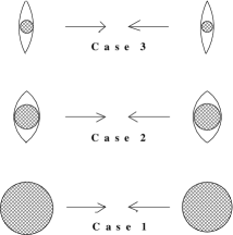
Figure 4: Schematic plot of two colliding particles. Case 1 corresponds to non-relativistic relative velocities. Case 2 corresponds to moderate relative velocities: particles suffering 50% contractions. Case 3 corresponds to high relative velocities: particles suffering 75% contractions. The balls are indicated by the hatched inscribed circles. The rest of the material constitute the rings.

With increasing energy, it seems that the proton is further squeezed. The ring gets flatter and wider so as to reduce the size of the hole while preserving its outer diameter. The ball now closing the hole is smaller. The total volume of the proton gets reduced. Naturally the mass and the charge distributions get denser and their partitioning between the two components vary. However, since the charge density in a proton tails off rapidly, the ring carries very little charge.

In the following qualitative analysis the ring is ignored. The modified scenerio is that with increasing energy a spherical proton remains spherical but gets smaller. The densities of mass and charge increase. The proton thus gets more and more compact. $r^{2}\rho_{20}$ and $r^{2}\rho_{40}$ in Figure 5 show the radial charge densities at $20\%$ and $40\%$ reductions of the rms radii respectively. Compared to the unreduced density $r^{2}\rho_{00}$ they are laterally contracted and vertically elongated.

Figure 5: Plot of $r^{2}\rho(r)$ in arbitrary units as a function of r in units of fm. For $r^{2}\rho_{00}$,   $\bar{r_{0}}$ = 0.005 & $\bar{r_{1}}$ = 0.8. For $r^{2}\rho_{20}$ these have the values 0.004 & 0.64 respectively and for $r^{2}\rho_{40}$ these values are 0.003 & 0.48.

Corresponding $p-p$ interaction potentials $V_{20}$ and $V_{40}$ are plotted along with $V_{00}$, the non-relativistic potential, in Figure 6.

Figure 6: Plot of the interparticle potential V in units of MeV as a function of the interparticle separation R in units of fm. For $V_{00}$ $\bar{r_{0}}$ = 0.005 & $\bar{r_{1}}$ = 0.8. For $V_{20}$ these have the values 0.004 & 0.64 respectively and for $V_{40}$ these values are 0.003 & 0.48.

They also display similar deformations. The process continues with decreasing size of the proton associated with increasing energy. The peak of the potential is attained at $R=0$. It is about $4\times 10^{5}MeV$ for a proton at rest or with non-relativistic energy.

Since the interaction between two reducing spheres goes on changing, the data collected from scattering experiments performed at different relativistic energies cannot be correlated unless the change of potential with energy is taken into consideration.

With increasing energy of collision the participants become more massive, very compact and extremely hard. Their fundamental ingredients are glued together more strongly. They are reluctant to leave their progressively reducing confines. Consequently, the colliding particles strongly resist disintegration under direct impact. Relativistic effects are comparatively less pronounced for a heavy nucleus carrying higher momentum with lower velocity. Collision between them may result in splintering into their constituent particles rather than totally disintegrating into their basic elements.

A 3-body collision may be induced by injecting a proton plasma or hydrogen atoms between two beams of colliding nuclei. From the centre-of-mass such a proton appears stationary. It is ‘soft’. The high speed nuclei are hard hitters. Some of the soft protons may get caught between them and be smashed.

If proton beams are used, the probability of a head-on collision gets reduced. A nucleus with mass number $M$ has a cross-section $M^{2/3}$ times that of a proton. The probability of two such nuclei colliding is $M^{4/3}$ times that of two protons.

The soft protons injected into the collision chamber must neither be too dense nor too thin. In a thick cloud most of the beam protons will hit plasma protons in 2-body collisions. From the centre-of-mass both will appear to be moving at half the beam proton’s speed. It will result in a collision between two hard protons. On the other hand, if the plasma is too thin, the colliding protons will find it difficult to get a soft proton in-between them.

Slower protons are preferable. They spend more time in the collision chamber and have better opportunities of capturing soft protons. But they must be energetic enough to smash the captive ones. Even then, 3-body events may occur infrequently and a successful experiment will require sensitive detector systems.

The ultimate result of a collision experiment depends upon the answer to yet another question that still persists: ‘what happens when a soft proton is smashed?’ Do the elementary particles constituting it fly off in different directions, or does it get flattened out and subsequently bounces back into its original form? Successful decomposition of a proton depends upon how much concussion the gluonic binding can withstand.

References

- (1) J.Jeans, Mathematical Theory of Electricity and Magnetism, (Cambridge University Press, Cambridge, 1958)
- (2) E.Fermi, Z.Phys. 60, 320 (1930)
- (3) A.Mukherji, Ph.D. thesis (University of Calcutta, Kolkata, India, 1960)
- (4) J.C.Slater, Quantum Theory of Molecules and Solids, Vol. I, (McGraw-Hill, New York, 1963)
- (5) A.Mukherji and P.Rudra, Ind.J.Phys., A54,5 (1980)
- (6) R.V.Reid, Ann.Phys.(NY), 50,411(1968)
- (7) R.M.Littauer, H.F.Schopper and R.R.Wilson, Phys.Rev.Lett., 7, 144 (1961)