Quantum Zeno dynamics: mathematical and physical aspects

Abstract

If frequent measurements ascertain whether a quantum system is still in its initial state, transitions to other states are hindered and the quantum Zeno effect takes place. However, in its broader formulation, the quantum Zeno effect does not necessarily freeze everything. On the contrary, for frequent projections onto a multidimensional subspace, the system can evolve away from its initial state, although it remains in the subspace defined by the measurement. The continuing time evolution within the projected “quantum Zeno subspace” is called “quantum Zeno dynamics:” for instance, if the measurements ascertain whether a quantum particle is in a given spatial region, the evolution is unitary and the generator of the Zeno dynamics is the Hamiltonian with hard-wall (Dirichlet) boundary conditions. We discuss the physical and mathematical aspects of this evolution, highlighting the open mathematical problems. We then analyze some alternative strategies to obtain a Zeno dynamics and show that they are physically equivalent.

,

1 Introduction: philosophy, history and physics

Zeno was a sophist philosopher, and a native of Elea, in Southern Italy. The quantum Zeno effect is named after him [117]. In this article we will discuss the physical and mathematical aspects of this phenomenon and its dynamical features.

Zeno put forward some famous paradoxical arguments against motion. We shall focus on one of these, according to which a sped arrow does not move, and analyze under which conditions an evolving quantum state may not move. We will start by framing Zeno’s arguments and their quantum mechanical counterparts in the proper philosophical, historical, cultural and physical context. This is a technical article, that will be (hopefully) read by physicists and mathematicians, yet we deem it appropriate to start from a genuine humanistic perspective.

1.1 Historical and philosophical prelude

Zeno was born about 488 BC in Elea, a small town not far from Naples, in the Mediterranean region called “Magna Graecia”. He was a prominent figure of the Eleatic school of philosophy, founded by Parmenides, of whom he was the favorite disciple. They believed that senses are deceptive and motion and change mere illusions: there is only one Truth (“being”) that is static, does not change and cannot be decomposed into parts or smaller entities. It is therefore indivisible and does not develop. This view contrasted with the notion of reality of Pythagoras and Heraclitus, who believed in a world of change and “becoming” and started revealing the power of thought and mathematics, on which modern science stands [151, 152, 66].

Zeno’s arguments were subtle and profound and aimed at bringing to light some paradoxical aspects of common sense and of the notion of a reality in continuous change. Some of these arguments directly deal with motion and one in particular will concern us here: a flying arrow is at rest. Indeed, at any given moment the arrow is in a portion of space equal to its own length, and therefore is at rest at that moment. Therefore, at every instant the arrow is motionless in a given position and the “sum” of these positions of rest is not a motion. Notice that, according to the original sources [8], no direct mention is made to the act of observation. Yet, implicitly, Zeno argued against our sensorial (and therefore deceptive) perception of movement.

Parmenides and Zeno went to Athens to discuss their ideas with Plato and Aristotle. We learn from Plato that at the time of that trip Zeno was about 40 years old, Parmenides about 65 and the pupil put all his energy in defending the view of his master. However, the two Eleatics were defeated (those were times when solidity of argumentation made a difference in philosophical and political discussions). Although many ancient writers refer to Zeno’s ideas, none of his writings survives, so that most of what we know of him comes from what Aristotle wrote [8]. This is like learning about a manuscript by reading a (negative) referee report, although an authoritative one. See Figure 1.

Figure 1: The School of Athens was painted by Raphael between 1509 and 1510 (in the frescoed Room of the Signature, one of Raphael’s rooms, in the Vatican Museums). All the protagonists of our story appear in this fresco. Parmenides is standing at the center-left, in a yellow shirt. Heraclitus (portrayed with Michelangelo’s features) is sitting at the center, his hand holding his head. Pythagoras, dressed in white and red, writes in a book, at the front-left. Zeno is at the very left, with a white beard, partially hidden by a putto (the baby holding a book): curiously, he looks older than his master Parmenides (although, according to Plato [8], he was twenty-five years younger). Plato and Aristotle are the dominant figures at the center of the painting and Raphael himself is standing at the very right, looking at us; he is almost hidden by Sodoma. (Courtesy Vatican Museums.)

Plato calls Zeno the inventor of dialectic: his arguments foreran the seemingly paradoxical method of proof that is known nowadays as reductio ad absurdum. It is therefore not surprising that Zeno is considered a precursor of sophism. The implication of the word sophist has changed greatly over time, running from its original meaning. Initially, it was a highly complimentary term, referred to someone who conveyed knowledge and wisdom (“sophia”) to his disciples. Eventually, by the time of Plato and Aristotle, the word had taken on negative connotations, usually referring to someone who used the arts of debate and rhetoric in order to deceive, or to support fallacious reasoning. In some modern Indo-European languages, words that have the same root as “sophisticator” have acquired a very negative meaning. In the Webster’s dictionary one finds that “echoes of Sophism survive today in the language theory of Jacques Derrida and other postmodern rhetoricians who teach that language ought to be deconstructed in order to unpack the intentions of “sophisticated” communicators.” Contemporary physics has sometimes, righteously, a difficult relationship with postmodern philosophy [167, 180].

Yet this inherited negative attitude does not render justice to Zeno, whose paradoxes have inspired philosophers for over two millennia, challenged mathematicians for a few hundred years, and puzzled physicists for the last 30 years. Many great thinkers looked for a way out of the paradoxes. Kant, Hume, Hegel and many others proposed solutions to Zeno’s paradoxes, pondering over the meaning of space, time and our forms of perception. Although these solutions were ultimately not accepted by modern mathematics and science, they helped shaping our modern concepts and rigorous definitions: our ideas of space, time, motion, infinite, infinitesimal, line, point, derivative and measure would not be the same without Zeno’s input. After two thousand years of continual refutation, his arguments made the foundation of modern mathematics. Rigorous definitions are unavoidable if one wants to rely on a logically consistent mathematical scheme and does not want to fall into contradictions.

It is probably fairly accurate to say that Zeno’s problems stem from human efforts to comprehend the infinite. Nowadays it is common to hear, in mathematics and physics circles, that Zeno’s arguments are based on false assumptions and that no Zeno-like paradoxes are present within modern mathematics. We venture to disagree, not on the conclusions, but on the premises: modern mathematics was created in order to avoid those questions that Zeno posed, in exactly the same way as modern set theory carefully avoids the use of Russell’s set of sets. Sped arrows move, runners catch tortoises, one can pass an infinite number of points in a finite time and our concepts of infinitesimal, finite and infinite have been adapted to our need to arrive at a consistent description of motion [156]. Clearly, no subsequent logically consistent system could afford to ignore Zeno’s paradoxes, but of course it would have been impracticable to accept passively a doctrine like that of Elea. When we describe the motion of a ball in terms of Newton’s law or the evolution of a wave function in terms of Schrödinger’s equation, we stand on the shoulders of thinkers who solved seemingly irreconcilable contradictions.

1.2 The quantum Zeno effect

The afore-mentioned Zeno’s paradox will be the object of the present investigation: A sped arrow will never reach its target, because when we look at the arrow, we see that it occupies a portion of space equal to its own size. At any given moment the arrow is therefore immobile, and by summing up many such “immobilities” it is impossible, according to Zeno, to obtain motion. It is amusing that quantum mechanical systems, when observed, behave in a way that is reminiscent of this paradox.

Frequent measurement slow the evolution of a quantum system, hindering transitions to states different from the initial one. This phenomenon, known as the quantum Zeno effect (QZE) [117, 179, 18, 87], is a consequence of general features of the Schrödinger equation, that yield quadratic behavior of the survival probability at short times [124, 70, 44].

Von Neumann [179] was the first to understand the far-reaching outcomes of the short-time evolution and bring to light the essentials of the Zeno phenomenon. However, he was focusing on quantum thermodynamics and his conclusions were forgotten for 35 years, when Beskow and Nilsson in a brilliant article [18] argued that frequent position measurements, implicitly carried out by a bubble chamber on an unstable particle, could prevent its decay. These ideas were corroborated by Khalfin [87], 10 years after his seminal work on the long-time features of quantum evolutions [85, 86], and were finally put on firm mathematical ground by Friedman [58].

At the same time, there was a widespread mathematical interest on the convergence of the Trotter-Kato product formula [173, 174, 82, 69]. Mathematicians focused on the limit of product formulas when the potential is singular or the Hamiltonian unbounded [23, 65, 59, 63, 31, 64, 157, 158, 159, 110, 32, 33]. These limits and their properties are indeed of great importance in the study of quantum dynamical semigroups and may contain the germs of irreversibility. Their relevance is therefore twofold, as they have remarkable consequences both in mathematical physics and operator theory.

Finally, these ideas were gathered by Baidyanaith Misra and George Sudarshan in their pioneering article [117], that introduced, among other things, the classical allusion to the Eleatic philosopher. The paper by Misra ad Sudarshan is also amusing in its own right: it blends rigorous mathematics with subtle and often ironical remarks about philosophy and cats. Since then, the QZE received constant attention by theorists, who explored different facets of the phenomenon.

The Zeno problem was considered an academic one until 1988, when Cook [26] proposed a test with oscillating systems, rather than on bona fide unstable ones. This was a concrete idea, that revived the subject and led to the celebrated experimental test by Itano et al a few years later [76]. The discussion that followed [145, 144, 77, 146, 75, 57, 139, 1, 138, 162, 14, 12, 88, 160, 112, 161, 101, 36, 71, 183] provided insight and new ideas, eventually leading to new experimental tests. The QZE was successfully checked in a variety of different situations, on experiments involving photon polarization [93], nuclear spin isomers [122], individual ions [10, 172, 188, 9], optical pumping [118], NMR [189], Bose-Einstein condensates [168] and new experiments are in preparation with neutron spin [79, 148] and superconducting qubits [80, 178]. One should also emphasize that the first experiments were not free from interpretational problems. Some of these were successfully solved (e.g., the issue of the so-called “repopulation” of the initial state [126] was first avoided in [10]), but some authors (sensibly) argued that the QZE had not been successfully demonstrated on bona fide unstable systems, as in the seminal proposals. Indeed, all the above mentioned experiments deal with finite (oscillating) systems, whose Poincaré time is finite. The analysis of the evolution at short times becomes more complicated when one considers unstable systems [111, 13, 41, 104, 81, 42, 3]: in such a case, novel and somewhat unexpected phenomena come to light. There were also noteworthy early attempts at interpreting preexisting experimental data on unstable particle decay [175]. However, only two experiments have been successfully performed so far on unstable systems, both by Mark Raizen’s group. In the first one [186] the presence of the short-time non-exponential region was brought to light, while in the second one [53] the quantum Zeno effect and its inverse were demonstrated. It is worth emphasizing that recent experimental demonstrations of the QZE are driven by interest in fundamental physics, but also by practical applications, such as efficient preservation of spin polarization in gases [122, 123], dosage reduction in neutron tomography [35] and control of decoherence in quantum computing [55, 49, 154, 72]. The last ten years have witnessed a number of very interesting ideas on the quantum Zeno effect as well as on possible applications [19, 24, 193, 12, 74, 194, 36, 40, 114, 115, 91, 2, 27, 107, 97, 171, 62, 108]. Some recent proposals, aimed at countering the detrimental effects of decoherence, deal with closely related quantum dynamics, in which the quantum measurements are frequent but not infinitely frequent [127, 128, 187, 25, 113, 190, 140, 116, 129]. The whole field is very active.

1.3 Quantum Zeno dynamics and quantum Zeno subspaces

Although all the afore-mentioned experiments invigorated studies on this issue, they essentially deal with one-dimensional projections (and therefore with what we might call one-dimensional Zeno effect): the system is forced to remain in its initial state. However, the QZE does not necessarily freeze everything. On the contrary, for a projection onto a multidimensional subspace, the system can evolve away from its initial state, although it remains in the subspace defined by the “measurement.” This continuing time evolution within the projected “Zeno subspace” we call quantum Zeno dynamics and is the central topic of this paper. It is often overlooked, although it is readily understandable in terms of the seminal theorem by Misra and Sudarshan [117]. One PACS number is now devoted to the quantum Zeno dynamics. Interestingly, less than one decade ago, an anonymous referee asked that the expression “quantum Zeno dynamics” be removed from the title of one of our articles. Times change, PACS numbers too.

We shall also discuss an interesting idea that has been repeatedly put forward in the mathematical and physical literature: Zeno dynamics yields ordinary constraints. In particular, suppose a system has Hamiltonian $H$ and the (frequent) measurement is checking that the system is within a particular spatial region. Then the Zeno dynamics that results is governed by the same Hamiltonian, but with Dirichlet boundary conditions on the boundary of the spatial region associated with the projection.

No experiments have been performed so far in order to check the multidimensional Zeno effect and the Zeno dynamics. However, these ideas might lead to remarkable applications, e.g. in the control of decoherence. For this reason, we shall explicitly look at some simple finite-dimensional examples of Zeno dynamics, in order to show how to freeze the dynamics of the simplest multidimensional system: a qubit.

1.4 Outline

This review article is organized as follows. We take a physicist’s approach in Secs. 2-4, where the QZE is introduced and discussed without spelling out implicit hypotheses and with no rigor in the derivations. The mathematics behind the QZE is discussed in Secs. 5-12. We focus here on the state of the art and explain what are the main mathematical difficulties and open problems. We finally turn to the practical applications of the QZE in Secs. 13-14: we show that it can be used in order to control the quantum dynamics and give three alternative (but physically equivalent) derivations of the Zeno subspaces. We conclude with an outlook in Sec. 15.

The path we will choose to describe the QZE will depend on our taste, for both its physical and mathematical aspects. A physically oriented reader can skip Secs. 5-12. A mathematically oriented reader can instead skip Secs. 13-14. However, we believe that a thorough comprehension of the Zeno phenomena, its implications and potential applications, can only be gained by combining physical and mathematical insight.

2 One-dimensional case

2.1 Fundamentals

Let a quantum system be prepared, at time $t=0$, in the pure state $|\psi_{0}\rangle$, a normalized vector in the Hilbert space ${\cal H}$. The system evolves under the action of the total Hamiltonian $H$. The quantities

$${\cal A}(t) = \langle\psi_{0}|\psi_{t}\rangle=\langle\psi_{0}|\mathrm{e}^{-iHt}|\psi_{0}\rangle,$$ (1)

$$p(t) = |{\cal A}(t)|^{2}=|\langle\psi_{0}|\mathrm{e}^{-iHt}|\psi_{0}\rangle|^{2},$$ (2)

are called survival amplitude and probability, respectively, and represent the amplitude and probability that the quantum system is found in the initial state $|\psi_{0}\rangle$ at time $t$. An elementary expansion at short times yields a quadratic behavior

$$p(t)=1-t^{2}/\tau_{\rm Z}^{2}+\ldots,\qquad\tau_{\rm Z}^{-2}\equiv\langle\psi_{0}|H^{2}|\psi_{0}\rangle-\langle\psi_{0}|H|\psi_{0}\rangle^{2},$$ (3)

where $\tau_{\rm Z}$ is the “Zeno time,” a (sometimes very inaccurate) quantitative estimate of the duration of the short-time quadratic behavior. Notice that if one decomposes the total Hamiltonian into a free and an interaction part

$$H = H_{0}+H_{\rm int},$$

$$H_{0} = PHP+QHQ,\qquad H_{\rm int}=PHQ+QHP,$$ (4)

where $P=\left|\psi_{0}\right\rangle\left\langle\psi_{0}\right|$ and $Q=1-P$, the initial state is an eigenstate of the free Hamiltonian, that is also completely off-diagonal with respect to the interaction

$$H_{0}\left|\psi_{0}\right\rangle=\omega_{0}\left|\psi_{0}\right\rangle,\qquad\left\langle\psi_{0}\right|H_{\rm int}\left|\psi_{0}\right\rangle=0.$$ (5)

The Zeno time reads then

$$\tau_{\rm Z}^{-2}=\langle\psi_{0}|H_{\rm int}^{2}|\psi_{0}\rangle$$ (6)

and depends only on the square of the interaction Hamiltonian. While the Fermi golden rule [50, 51, 52] “picks” only the on-shell contribution of the interaction, the Zeno time “explores” (in agreement with the time-energy uncertainty relation) all possible intermediate states, by virtue of the completeness relation

$$\langle\psi_{0}|H_{\rm int}^{2}|\psi_{0}\rangle=\langle\psi_{0}|H_{\rm int}QH_{\rm int}|\psi_{0}\rangle=\sum_{n\neq 0}\langle\psi_{0}|H_{\rm int}|n\rangle\langle n|H_{\rm int}|\psi_{0}\rangle,$$ (7)

where $|n\rangle$ (with $\left|0\right\rangle=\left|\psi_{0}\right\rangle$) is an eigenbasis of the free Hamiltonian $H_{0}$. The decomposition (4) is at the heart of the Lippmann-Schwinger equation [153] and plays an important role in quantum field theory.

Let us now carry out $N$ measurements at time intervals $\tau=t/N$, in order to check whether the system is still in its initial state. If every time the measurement has a positive outcome and the system is found in its initial state, the wave function “collapses” and the evolution starts anew from $|\psi_{0}\rangle$. The survival probability after the $N$ measurements reads

$$p^{(N)}(t) = p(\tau)^{N}=p(t/N)^{N}$$ (8)

$$\stackrel{{\scriptstyle N\;{\rm large}}}{{\sim}} \left[1-(t/N\tau_{\rm Z})^{2}\right]^{N}\sim\exp(-t^{2}/N\tau_{\rm Z}^{2})\stackrel{{\scriptstyle N\rightarrow\infty}}{{\longrightarrow}}1,$$

where $t=N\tau(<\infty)$ is the total duration of the experiment. The Zeno evolution is pictorially represented in Fig. 2. The $N\rightarrow\infty$ limit was originally named limit of “continuous observation” by Misra and Sudarshan and regarded as a paradoxical results: infinitely frequent measurements halt the quantum mechanical evolution and freeze the system in its initial state. Zeno’s quantum mechanical arrow (the wave function), sped by the Hamiltonian, does not move, if it is continuously observed. The QZE is not considered paradoxical nowadays: it is a consequence (admittedly, a curious one) of the quantum mechanical evolution law. Clearly, if one considers real physical measurement processes, effectively described in terms of projection operators, the $N\rightarrow\infty$ limit must be considered as a convenient mathematical abstraction [125, 176, 141, 73], but the evolution is indeed slowed down for sufficiently large $N$. An interesting alternative viewpoint can be found in [17], where the “continuous” measurement is implemented in terms of a dynamical constraint. From such a perspective, no $N\to\infty$ limit need be considered. The constraint picture that arises from the QZE is discussed in [38].

As a very simple example consider a two-level system with Hamiltonian

$$H=H_{\rm int}=\Omega\sigma_{1},$$ (9)

where $\Omega\in\mathbb{R}$ and $\sigma_{1}$ is the first Pauli matrix. Let the initial state be $|\psi_{0}\rangle=|+\rangle$, the positive eigenstate of the third Pauli matrix $\sigma_{3}$. The survival amplitude, survival probability and Zeno time read

$${\cal A}(t)=\langle+|\mathrm{e}^{-i\Omega t\sigma_{1}}|+\rangle=\cos\Omega t,\qquad p(t)=\cos^{2}\Omega t,\qquad\tau_{\rm Z}=\Omega^{-1},$$ (10)

respectively. For large $N$,

$$p^{(N)}(t)=\left(\cos\frac{\Omega t}{N}\right)^{2N}\sim\left(1-\frac{\Omega^{2}t^{2}}{2N^{2}}\right)^{2N}\sim\mathrm{e}^{-\Omega^{2}t^{2}/N}\stackrel{{\scriptstyle N\to\infty}}{{\longrightarrow}}1.$$ (11)

The limit (8) is therefore valid and one obtains a nice example of QZE. Observe that in this case $\tau_{\rm Z}$ does yield a good estimate of the duration of the short time region.

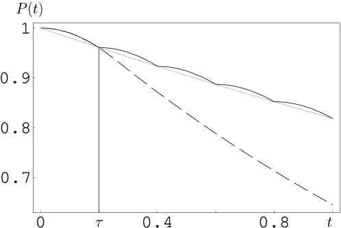
Figure 2: The quantum Zeno effect. The dashed (full) line is the survival probability without (with) measurements. The total duration of the experiment is $t=1$ and there are $N=5$ measurements, so that $\tau=0.2$. In the limit of “continuous observation” ($N\to\infty$, $t$ finite), $p(t)\to 1$. The grey line is the interpolating function in the far r.h.s. of Eq. (14).

2.2 A few preliminary comments and the inverse Zeno effect

Let us briefly comment on the seemingly innocuous derivation of the preceding subsection.

2.2.1 Short-time dynamics.

The QZE is ascribable to the following mathematical feature of the Schrödinger equation: in a short time $\delta\tau\propto 1/N$, the phase of the wave function evolves like $\mbox{O}(\delta\tau)$, while the probability changes by $\mbox{O}(\delta\tau^{2})$, so that

$$p^{(N)}(t)=\left[1-\mbox{O}(1/N^{2})\right]^{N}\stackrel{{\scriptstyle N\rightarrow\infty}}{{\longrightarrow}}1.$$ (12)

This is sketched in Fig. 3.

Figure 3: Short-time evolution of phase and probability. The phase of the evolved wave function is linear in time, while the probability loss is quadratic.

2.2.2 Quantum measurements.

In the preceding analysis, the measurements simply ascertain whether the system is in its initial pure state. In other words, the von Neumann measurement can be described by the one-dimensional projector

$$P=|\psi_{0}\rangle\langle\psi_{0}|.$$ (13)

This notion will be extended in the following section, where more general measurements will be considered. This will lead us to the notion of Zeno subspaces.

2.2.3 Rigor.

No care was taken of subtle mathematical issues, such as for instance the validity of the asymptotic expansion (3). Loosely speaking, we required finite moments of $H$ in the initial state and implicitly assumed that the Hamiltonian $H$ be bounded. In a general setting, the features of the Hamiltonian must be spelled out and it is not obvious that the series (3) will converge, or it is even defined, as it involves higher order moments of the field Hamiltonian in the cumulant expansion. An explicit example involving the hydrogen atom can be found in [41]. See also [164, 165], were the role of the form factors of the interaction is scrutinized.

The quantum Zeno effect in a quantum field theoretical framework has been investigated only relatively recently [13, 41, 104, 81, 42, 3, 5]. The features of the short-time evolution are not obvious, in particular when the convergence of the expansions cannot be proven.

There are other problems that are largely unexplored. Among these, the conditions that lead to a non-quadratic evolution at short times [29, 121, 119]. Interestingly, these issues are relevant in quantum tunneling [120].

2.2.4 The Zeno time.

In many situations, the Zeno time (3) yields a misleading estimate: strictly speaking, $\tau_{\rm Z}$ is nothing but the convexity of $p(t)$ in the origin. If the asymptotic series (3) is nasty, one needs a much more refined estimate of the duration of the short-time quadratic region [41, 5]. This leads us to the final comment:

2.2.5 Inverse Zeno effect: Heraclitus vs Zeno.

Interfering with a transition at a later stage in its progress leads to the opposite phenomenon, known as the inverse or anti-Zeno effect, in which decay is accelerated. Both effects have recently been seen in the same experimental setup [53]. Let us briefly describe this interesting aspects of quantal evolutions. Rewrite (8) as

$$p^{(N)}(t)=p(\tau)^{N}=\exp(N\log p(\tau))=\exp(-\gamma_{\rm eff}(\tau)t),$$ (14)

where we introduced the effective decay rate

$$\gamma_{\rm eff}(\tau)\equiv-\frac{1}{\tau}\log p(\tau).$$ (15)

The far right hand side of (14) interpolates the survival probability when $N$ measurements are performed, namely it intercepts the survival probability at its cusps, when the system is projected back onto its initial state (see Fig. 2).

Observe that in the region of validity of the expansion (3) $\gamma_{\rm eff}$ is a linear function of $\tau$

$$\gamma_{\rm eff}(\tau)\sim\tau/\tau_{\rm Z}^{2},\qquad\mbox{for}\quad\tau\to 0.$$ (16)

For example, with the Hamiltonian (9) and the initial state $|+\rangle$, one gets from Eq. (11)

$$p^{(N)}(t)\sim\mathrm{e}^{-\Omega^{2}t^{2}/N}=\mathrm{e}^{-(\Omega^{2}\tau)t}=\mathrm{e}^{-\gamma_{\rm eff}(\tau)t},$$ (17)

with $\tau=t/N$ and $\gamma_{\rm eff}(\tau)\sim\Omega^{2}\tau=\tau/\tau_{\rm Z}^{2}$.

If the system is unstable one expects to recover the “natural” decay rate $\gamma$, in agreement with the Fermi golden rule, for sufficiently long times, i.e., after the initial quadratic region is over

$$\gamma_{\rm eff}(\tau)\stackrel{{\scriptstyle{\rm``large"}\tau}}{{\longrightarrow}}\gamma.$$ (18)

The physical meaning of the mathematical expressions $\tau\to 0$ and “large” $\tau$ in the preceding formulas is in itself an interesting issue, that entails the definition of a timescale [39, 42]. This difficult and delicate problem will not be discussed here. Suffices it to say that when a quantum field theoretical description is necessary, $\tau_{\rm Z}$ is not the right timescale. We shall neither scrutinize here the features of the quantum mechanical evolution law at short [18, 87] and long [106, 54, 68, 130, 85, 86] times, nor analyze the validity of the Weisskopf-Wigner approximation [61, 181, 182, 20] and the onset to the Fermi “golden rule” [50, 51, 52]. These topics are summarized and discussed in [124].

Consider now an unstable system, with decay rate $\gamma$. If a finite time $\tau^{*}$ exists such that

$$\gamma_{\rm eff}(\tau^{*})=\gamma,$$ (19)

then by performing measurements at time intervals $\tau^{*}$ the system decays according to its “natural” lifetime, as if no measurements were performed. By Eqs. (19) and (15) one gets

$$p(\tau^{*})=\mathrm{e}^{-\gamma\tau^{*}},$$ (20)

i.e., $\tau^{*}$ is the intersection between the curves $p(t)$ and $\mathrm{e}^{-\gamma t}$ [39]. Figure 4(a) illustrates an example in which such a time $\tau^{*}$ exists. By looking at Fig. 4(b), it is evident that if $\tau=\tau_{1}<\tau^{*}$ one obtains a QZE. Vice versa, if $\tau=\tau_{2}>\tau^{*}$, one obtains an inverse Zeno effect (IZE). In this sense, $\tau^{*}$ can be viewed as a transition time from a quantum Zeno to an inverse Zeno regime. Paraphrasing Misra and Sudarshan, we can say that $\tau^{*}$ determines the transition from Zeno (who argued that a sped arrow does not move) to Heraclitus (who replied that everything flows).

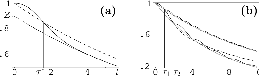
Figure 4: (a) Time $\tau^{*}$ separates the quantum Zeno from the Heraclitus (or inverse Zeno) regime. The full line is the survival probability $p(t)$, that tends to the asymptotic exponential ${\cal Z}\mathrm{e}^{-\gamma t}$ for large $t$ (dotted line, ${\cal Z}$ stemming from wave-function renormalization, see [39]); the dashed line is the exponential $\mathrm{e}^{-\gamma t}$. (b) Quantum Zeno vs inverse Zeno (or Heraclitus) effect. The dashed line is the undisturbed survival probability $p(t)$. The full black lines represent the survival probabilities when measurements are made at time intervals $\tau$ and the dotted grey lines their exponential interpolations, according to (14). For $\tau_{1}<\tau^{*}<\tau_{2}$ the effective decay rate $\gamma_{\rm eff}(\tau_{1})$ [$\gamma_{\rm eff}(\tau_{2})$] is smaller [larger] than the “natural” decay rate $\gamma=\gamma_{\rm eff}(\tau^{*})$, yielding QZE [IZE].

The Zeno-Heraclitus transition and the onset to the inverse Zeno effect were discussed by different authors [94, 155, 135, 84, 160, 170, 137, 47, 89, 43, 90, 39]. In some cases, $\tau^{*}$ does not exist and no inverse Zeno effect can take place [39]. In the remaining part of this article we will assume that $N$ is sufficiently large, so that we are in the Zeno regime, and that the $N\to\infty$ limit can be taken.

3 Finite-dimensional projections: the quantum Zeno subspaces

We now give a broader definition of measurement and generalize the notion of QZE. This can be done with the help of Lüders’s postulate [98], that suitably extends von Neumann’s [179].

A measurement is called “incomplete” if some outcomes are lumped together, for instance because the measuring apparatus has insufficient resolution. The projection operator that selects a given lump is therefore multidimensional and in this sense the information gained on the measured observable is incomplete. By contrast, a (selective) complete measurement yields a definite outcome of the observable being measured. In the discussion of Sec. 2 the measurements were selective and complete, because the system was found in $|\psi_{0}\rangle$.

Let the evolution of the quantum system in the Hilbert space ${\cal H}$ be governed by the unitary operator $U(t)=\exp(-iHt)$, where $H$ is a time-independent Hamiltonian. We assume that the projection operator $P$ that describes the measurement does not commute with the Hamiltonian, $[P,H]\neq 0$ and that $\mathrm{Tr}P=s<\infty$. The measurement therefore ascertains whether the system is in the $s$-dimensional subspace $P{\cal H}={\cal H}_{P}$. For instance, the reader can think of a finite, say $m$-dimensional Hilbert space. In such a case $H$ is a $m\times m$ matrix, with $\dim{\cal H}_{P}=s<m=\dim{\cal H}$.

It is convenient to discuss the evolution in terms of density matrices. The initial density matrix $\rho_{0}$ is taken to belong to ${\cal H}_{P}$ (state preparation)

$$\rho_{0}=P\rho_{0}P,\qquad\mbox{Tr}[\rho_{0}P]=1$$ (21)

and the state at time $\tau$ is

$$\rho(\tau)=U(\tau)\rho_{0}U^{\dagger}(\tau)$$ (22)

If we measure $P$ and the outcome is positive, the state, up to a normalization $p(\tau)$, changes into [98]

$$\rho(\tau) \rightarrow P\rho(\tau)P=PU(\tau)\rho_{0}U^{\dagger}(\tau)P$$ (23)

$$= V(\tau)\rho_{0}V^{\dagger}(\tau),\quad\qquad V(\tau)\equiv PU(\tau)P$$

and the survival probability in ${\cal H}_{P}$ reads

$$p(\tau) = \mbox{Tr}\left[U(\tau)\rho_{0}U^{\dagger}(\tau)P\right]=\mbox{Tr}\left[PU(\tau)P\rho_{0}PU^{\dagger}(\tau)P\right]$$ (24)

$$= \mbox{Tr}\left[V(\tau)\rho_{0}V^{\dagger}(\tau)\right].$$

Since $[P,H]\neq 0$, the Hamiltonian $H$ induces transitions out of ${\cal H}_{P}$ into ${\cal H}_{P}^{\perp}={\cal H}_{Q}$ $({\cal H}_{P}\oplus{\cal H}_{Q}={\cal H}$ and $P+Q=1$) and $p(\tau)$ is in general smaller than unity. There is, of course, a probability $q(\tau)=1-p(\tau)$ that the system has not survived (i.e., it has made a transition out of ${\cal H}_{P}$) and its state has changed, up to a normalization $q(\tau)$, into

$$\rho(\tau) \rightarrow Q\rho(\tau)Q=QU(t)\rho_{0}U^{\dagger}(t)Q$$ (25)

$$= V_{QP}(\tau)\rho_{0}V_{QP}^{\dagger}(\tau),\quad\qquad V_{QP}(\tau)\equiv QU(\tau)P.$$

The final state after the measurement is therefore a block diagonal matrix:

$$\rho_{0} \stackrel{{\scriptstyle{\rm unitary}}}{{\longrightarrow}} U(\tau)\rho_{0}U^{\dagger}(\tau)\stackrel{{\scriptstyle{\rm measurement}}}{{\longrightarrow}}\pmatrix{V(\tau)\rho_{0}V^{\dagger}(\tau)&0\cr 0&V_{QP}(\tau)\rho_{0}V_{QP}^{\dagger}(\tau)}.$$

The density matrix is reduced to a mixture and any possibility of interference between “survived” and “not survived” states is destroyed (complete decoherence).

We shall henceforth concentrate our attention only on the measurement outcome (23)-(24) and turn to the multidimensional Zeno effect. The state of the system after a (successful) series of $P$-observations at time intervals $\tau=t/N$ is

$$\rho^{(N)}(t)=V_{N}(t)\rho_{0}V_{N}^{\dagger}(t)/p^{(N)}(t),\qquad V_{N}(t)\equiv[PU(t/N)P]^{N}$$ (27)

and the survival probability to find the system in ${\cal H}_{P}$ is

$$p^{(N)}(t)=\mbox{Tr}\left[V_{N}(t)\rho_{0}V_{N}^{\dagger}(t)\right].$$ (28)

We have to study the limit

$$U_{\rm Z}(t)\equiv\lim_{N\to\infty}V_{N}(t)=\lim_{N\to\infty}\left[P\mathrm{e}^{iHt/N}P\right]^{N}.$$ (29)

This is easily computed by expanding

$$V_{N}(t) = \left[P\left(1-iHt/N+O\left(1/N^{2}\right)\right)P\right]^{N}$$ (30)

$$= P\left[1-iPHPt/N+O\left(1/N^{2}\right)\right]^{N}$$

$$\stackrel{{\scriptstyle N\to\infty}}{{\longrightarrow}} P\mathrm{e}^{-iPHPt}=U_{\rm Z}(t).$$

The dynamics is governed by the “Zeno” Hamiltonian $H_{\rm Z}\equiv PHP$ and the evolution is unitary in ${\cal H}_{P}$. We shall write

$$U_{\rm Z}(t)=P\exp(-iH_{\rm Z}t)$$ (31)

and speak of quantum Zeno dynamics in the quantum Zeno subspace ${\cal H}_{P}$. Notice that the one-dimensional result of the previous section is obtained when $\mbox{Tr}P={\cal H}_{P}=s=1$ (and then $H_{\rm Z}=$ constant = phase). The final state is

$$\rho(t)=\lim_{N\rightarrow\infty}\rho^{(N)}(t)=U_{\rm Z}(t)\rho_{0}U_{\rm Z}(t)^{\dagger}$$ (32)

and the probability to find the system in ${\cal H}_{P}$ is

$$\lim_{N\rightarrow\infty}p^{(N)}(t)=\mbox{Tr}\left[U_{\rm Z}(t)\rho_{0}U_{\rm Z}(t)^{\dagger}\right]=\mbox{Tr}\left[\rho_{0}P\right]=1.$$ (33)

This is the multidimensional QZE. If the particle is constantly checked for whether it has remained in ${\cal H}_{P}$, it never makes a transition to ${\cal H}_{P}^{\perp}$.

A few comments are in order. First, notice that for finite $N$ the dynamics (27)-(28) is not reversible. The dynamics becomes unitary and reversible in the $N\to\infty$ limit. The physical mechanism that ensures the conservation of probabilities within the relevant subspace hinges on the short time behavior of the survival probability: probability leaks out of the subspace ${\cal H}_{P}$ like $\tau^{2}$ for short times. The infinite-$N$ limit suppresses this loss. Finally, the analysis of this section is straightforward for finite systems and finite dimensional projectors. Things get much more complicated for infinite dimensional systems. One can then inquire under what circumstances $U_{\rm Z}(t)$ actually forms a group, yielding reversible dynamics within the Zeno subspace. The seminal paper by Misra and Sudarshan [117] showed that in general the dynamics in the $N\to\infty$ limit is governed by a semigroup and therefore bears the symptoms of irreversibility. The simple finite-dimensional example discussed in this section shows that irreversibility is not compulsory. Notice also that in the infinite dimensional case the meaning of $PHP$ must be defined and the self-adjointness of the Hamiltonian $H_{\rm Z}$ cannot be taken for granted.

We focused here on one quantum Zeno subspace ${\cal H}_{P}$. However, the notion of Zeno subspace and Zeno dynamics can be extended to a collection of projectors (an orthogonal resolution of the identity) [39]. See Sec. 13.1.

4 Infinite-dimensional case: position measurement

We now analyze the infinite dimensional case. We will not focus on the most general situation, but will rather study the Zeno dynamics for the simplest spatial projection, a position measurement on a free particle. We shall review and slightly modify the proof given in Refs. [34, 48].

Consider a free particle of mass $m$ in $d$ dimensions

$$H=\frac{\bm{p}^{2}}{2m}=-\frac{\Delta}{2m},\qquad U(t)=\mathrm{e}^{-iHt}.$$ (34)

The Hamiltonian $H$ is a positive-definite self-adjoint operator on ${\cal H}=L^{2}(\mathbb{R}^{d})$ and $U(t)$ is unitary. Given a compact domain $\Omega\subset\mathbb{R}^{d}$ with a nonempty interior and a regular boundary, we study the evolution of the particle when it undergoes frequent measurements defined by the projector

$$P=\chi_{\Omega}(\bm{x})=\int_{\Omega}\mathrm{d}^{d}\bm{x}\left|\bm{x}\right\rangle\left\langle\bm{x}\right|,\qquad P\psi(\bm{x})=\chi_{\Omega}(\bm{x})\psi(\bm{x}),$$ (35)

where

$$\chi_{\Omega}(\bm{x})=\left\{\begin{array}[]{l}1\quad\mbox{for }\bm{x}\in\Omega\\ 0\quad\mbox{otherwise}\end{array}\right.$$ (36)

is the characteristic function of the domain $\Omega$, and thought of as an operator, along with its complement $Q=1-P=1-\chi_{\Omega}(\bm{x})$, decomposes the space $L^{2}(\mathbb{R}^{d})$ into two orthogonal subspaces. We study the following process. We prepare a particle in a state with support in $\Omega$, let it evolve under the action of its Hamiltonian, perform frequent $P$ measurements during the time interval $[0,t]$, and study the evolution of the system within the Zeno subspace ${\cal H}_{P}=P{\cal H}$.

The Zeno dynamics evolution operator is given by the limit

$$U_{\rm Z}(t)=\lim_{N\to\infty}\left[V(t/N)\right]^{N},$$ (37)

where the (nonunitary) evolution operator $V$ is given in Eq. (23) and represents a single step (projection-evolution-projection) Zeno process. We now show that (37) yields the unitary evolution

$$U_{\rm Z}(t)=\exp(-iH_{\rm Z}t)P$$ (38)

generated by the Zeno Hamiltonian

$$H_{\rm Z}=-\frac{\Delta_{\Omega}}{2m},$$ (39)

whose domain is a proper subspace of $L^{2}(\Omega)$

$$D(H_{\rm Z})=\{\psi\in L^{2}(\Omega)\;|\;\Delta\psi\in L^{2}(\Omega),\psi(\partial\Omega)=0\},$$ (40)

$\partial\Omega$ being the boundary of $\Omega$ (hard-wall or Dirichlet boundary conditions).

One might rewrite Eq. (39) as

$$H_{\rm Z}\equiv\frac{{\bm{p}}^{2}}{2m}+V_{\Omega}(\bm{x}),\quad V_{\Omega}(x)=\left\{\begin{array}[]{l}0\qquad\mbox{~{}for }\bm{x}\in\Omega\\ +\infty\quad\mbox{otherwise}\end{array}\right..$$ (41)

In other words, the system behaves as if it were confined in $\Omega$ by rigid walls, inducing the wave function to vanish on the boundary of $\Omega$.

4.1 Proof

The matrix elements of the $d$-dimensional single-step propagator $V$ in Eq. (23) read (in the position representation)

$$G({\bm{x}},\tau;{\bm{y}}) = \left\langle\bm{x}\right|V(\tau)\left|\bm{y}\right\rangle$$ (42)

$$= \chi_{\Omega}(\bm{x})\left(\frac{m}{2\pi i\tau}\right)^{d/2}\exp\left[\frac{im(\bm{x}-\bm{y})^{2}}{2\tau}\right]\chi_{\Omega}(\bm{y}).$$

We will work in the eigenbasis $\{\left|{\bm{n}}\right\rangle\}$ of $H_{\rm Z}$ belonging to the eigenvalues $E_{\bm{n}}$

$$H_{\rm Z}\Psi_{\bm{n}}(\bm{x})=E_{\bm{n}}\Psi_{\bm{n}}(\bm{x}),\qquad\Psi_{\bm{n}}(\bm{x})=\left\langle\bm{x}\right|\bm{n}\rangle,$$ (43)

in the subspace $PL^{2}(\mathbb{R}^{d})\simeq L^{2}(\Omega)$. This is also the eigenbasis of $U_{\rm Z}(t)$. In this basis,

$$G_{\bm{m},\bm{n}}(\tau) = \left\langle\bm{m}\right|V(\tau)\left|\bm{n}\right\rangle$$ (44)

$$= \int_{\Omega}\mathrm{d}^{d}x\int_{\Omega}\mathrm{d}^{d}y\left(\frac{m}{2\pi i\tau}\right)^{d/2}e^{i\frac{m(\bm{x}-\bm{y})^{2}}{2\tau}}\Psi^{*}_{\bm{m}}(\bm{x})\Psi_{\bm{n}}(\bm{y})$$

$$= \int_{\Omega}\mathrm{d}^{d}x\;\Psi^{*}_{\bm{m}}(\bm{x})[\mbox{bound}+\mbox{stat}]+\mbox{b-s regions},$$ (45)

where we split the integral into three parts, representing respectively the contribution of the boundary $\bm{x}$ or $\bm{y}\in\partial\Omega$, the stationary part $\bm{x}=\bm{y}\in\Omega-\partial\Omega$, and the boundary points that are also stationary points (such points belong to the diagonal part of the intersection of the boundaries of the two domains $\Omega$ in (44), namely $\bm{x}=\bm{y}\in\partial\Omega$). We shall separately evaluate the three contributions in the small-$\tau$ limit, by introducing some smooth regularizing functions and splitting the integration domain into three parts, as shown in Fig. 5. Each regularizing function takes value one on a compact domain and smoothly vanishes outside.

Figure 5: Regularizers on the integration domain.

The first two terms can be evaluated by substituting $\bm{\xi}=\bm{y}-\bm{x}$, to obtain

$$G_{\bm{m},\bm{n}}(\tau) = \int_{\Omega}\mathrm{d}^{d}x\;\Psi_{\bm{m}}^{*}(\bm{x})\int_{\Omega-\bm{x}}\mathrm{d}^{d}\xi\left(\frac{m}{2\pi i\tau}\right)^{d/2}e^{i\frac{m\bm{\xi}^{2}}{2\tau}}\Psi_{\bm{n}}(\bm{x}+\bm{\xi}),$$ (46)

where

$$\Omega-\bm{x}=\{\bm{y}\;|\;\bm{x}+\bm{y}\in\Omega\}.$$ (47)

In order to compute the boundary term, we first observe that

$$e^{i\lambda\bm{\xi}^{2}}=\frac{\bm{\xi}\cdot\nabla e^{i\lambda\bm{\xi}^{2}}}{2i\lambda\bm{\xi}^{2}}$$ (48)

and then integrate by parts ($\lambda=m/2\tau$)

bound $$= \int_{\Omega}\mathrm{d}^{d}\xi\left(\frac{\lambda}{\pi i}\right)^{d/2}\Psi_{\bm{n}}(\bm{x}+\bm{\xi})\frac{\bm{\xi}\cdot\nabla e^{i\lambda\bm{\xi}^{2}}}{2i\lambda\bm{\xi}^{2}}$$ (49)

$$= \left(\frac{\lambda}{\pi i}\right)^{d/2}\left[\int_{\Omega}\mathrm{d}^{d}\xi\;\nabla\cdot\left(\frac{\Psi_{\bm{n}}(\bm{x}+\bm{\xi})\bm{\xi}e^{i\lambda\bm{\xi}^{2}}}{2i\lambda\bm{\xi}^{2}}\right)\right.$$

$$\qquad\qquad\left.-\int_{\Omega}\mathrm{d}^{d}\xi\;\nabla\cdot\left(\frac{\Psi_{\bm{n}}(\bm{x}+\bm{\xi})\bm{\xi}}{\bm{\xi}^{2}}\right)\frac{\bm{\xi}\cdot\nabla e^{i\lambda\bm{\xi}^{2}}}{(2i\lambda)^{2}\bm{\xi}^{2}}\right]$$

$$= \left(\frac{\lambda}{\pi i}\right)^{d/2}\left[\oint_{\partial(\Omega-\bm{x})}d^{d-1}S\;\frac{\Psi_{\bm{n}}(\bm{x}+\bm{\xi})\bm{\xi}\cdot\hat{\bm{u}}}{\bm{\xi}^{2}}\;\frac{e^{i\lambda\bm{\xi}^{2}}}{2i\lambda}\left(1+O(\lambda^{-1})\right)\right]$$

$$= \left(\frac{m}{2\pi i\tau}\right)^{d/2}\left[\oint_{\partial\Omega}d^{d-1}S\;\frac{\Psi_{\bm{n}}(\bm{y})(\bm{y}-\bm{x})\cdot\hat{\bm{u}}}{(\bm{y}-\bm{x})^{2}}\;\frac{e^{im(\bm{x}-\bm{y})^{2}/2\tau}}{im/\tau}\right.$$

$$\qquad\qquad\qquad\times\left(1+\;O(\tau)\right)\Bigg{]},$$

$\hat{\bm{u}}$ being the unit vector perpendicular to the boundary. We extended the integration domain to the whole $\Omega$ and did not explicitly write the regularizing function, that should multiply the integrand, as its action is trivial in this case. In the second equality, Eq. (48) was used again in order to obtain a higher-order volume integral with the same structure as the initial one. Since $\Psi_{\bm{n}}$ in Eq. (43) is an eigenfunction of $H_{\rm Z}$, whose domain is (40), one gets

$$\mbox{bound}=0.$$ (50)

The stationary contribution is obtained by expanding the integrand around $\bm{x}$

stat $$= \left(\frac{m}{2\pi i\tau}\right)^{d/2}\int\mathrm{d}^{d}\xi\;e^{i\lambda\bm{\xi}^{2}}$$ (51)

$$\times\left(\Psi_{\bm{n}}(\bm{x})+\nabla\Psi_{\bm{n}}(\bm{x})\cdot\bm{\xi}+\frac{1}{2!}\partial_{i}\partial_{j}\Psi_{\bm{n}}(\bm{x})\xi_{i}\xi_{j}+O(|\bm{\xi}|^{3})\right).$$

Observe that the contributions of the linear and quadratic (with $i\neq j$) terms in the integral vanish due to symmetry and one is left with

stat $$= \Psi_{\bm{n}}(\bm{x})+i\frac{\tau}{2m}\Delta\Psi_{\bm{n}}(\bm{x})+O(\tau^{2})$$ (52)

$$= \left(1-iE_{\bm{n}}\tau\right)\Psi_{\bm{n}}(\bm{x})+O(\tau^{2}),$$

where we used Eq. (43). Also in this case we did not explicitly write the regularizing function in the integrand, as its action is trivial.

Finally, we evaluate the contribution of the b-s region. Let us first see what happens in $d=1$. We take $\Omega=[0,a]$ and compute

$$\mbox{b-s region}=\left(\frac{\lambda}{\pi i}\right)^{1/2}\int_{0}^{a}\mathrm{d}x\int_{0}^{a}\mathrm{d}ye^{i\lambda(x-y)^{2}}\Psi^{*}_{m}(x)\Psi_{n}(y)\nu(x,y),$$ (53)

where $\nu(x,y)$ is a regularizing function that smoothly vanishes for $|x|,|y|>\epsilon$. We expand the eigenfunctions around the origin,

$$\Psi_{m}(x)=\Psi_{m}(0)+x\Psi^{\prime}_{m}(0)+O(x^{2})\sim x\Psi^{\prime}_{m}(0),\quad x\to 0,$$ (54)

where we made use of the fact that $\Psi_{m}$ is an eigenfunction of the Hamiltonian (39) and obeys Dirichlet boundary conditions (the calculation around the other boundary point $x\simeq y\simeq a$ is identical). Plugging into (53) and changing integration variables $\xi=(x-y)/\sqrt{2},\eta=(x+y)/\sqrt{2}$, we get

b-s region $$\sim \left(\frac{\lambda}{\pi i}\right)^{1/2}\int_{0}^{\epsilon}\mathrm{d}x\int_{0}^{x}\mathrm{d}y\;xy\;e^{i\lambda(x-y)^{2}}\Psi^{*^{\prime}}_{m}(0)\Psi^{\prime}_{n}(0)$$ (55)

$$= \left(\frac{\lambda}{\pi i}\right)^{1/2}\Psi^{*^{\prime}}_{m}(0)\Psi^{\prime}_{n}(0)\int_{0}^{\epsilon/\sqrt{2}}\mathrm{d}\eta\int_{0}^{\eta}\mathrm{d}\xi e^{i2\lambda\xi^{2}}(\eta^{2}-\xi^{2})$$

$$= \left(\frac{1}{\pi i}\right)^{1/2}\Psi^{*^{\prime}}_{m}(0)\Psi^{\prime}_{n}(0)\left(\frac{\sqrt{\pi i}}{24}\epsilon^{3}-\frac{i^{3/2}}{16\lambda}\epsilon-\frac{1}{12\lambda^{3/2}}+o(\lambda^{-3/2})\right)$$

$$= O(\tau^{3/2})+\epsilon O(\tau)+\frac{\epsilon^{3}}{24},$$

and by sending $\epsilon\to 0$ we obtain

$$\mbox{b-s region}=O(\tau^{3/2}).$$ (56)

Note that the residual $\epsilon O(\tau)$ contribution is due to the stationary points in $[0,\epsilon]^{2}$ and belongs to the bulk of Eq. (52).

In $d$ dimensions the proof is similar. By writing

b-s region $$= \left(\frac{\lambda}{\pi i}\right)^{d/2}\int_{\Omega}\mathrm{d}^{d}x\int_{\Omega}\mathrm{d}^{d}ye^{i\lambda(\bm{x}-\bm{y})^{2}}\Psi^{*}_{\bm{m}}(\bm{x})\Psi_{\bm{n}}(\bm{y})\nu(\bm{x},\bm{y}),$$ (57)

$$\simeq \left(\frac{\lambda}{\pi i}\right)^{d/2}\int_{\omega_{\epsilon}}\mathrm{d}^{d}x\int_{\omega_{\epsilon}}\mathrm{d}^{d}ye^{i\lambda(\bm{x}-\bm{y})^{2}}\Psi^{*}_{\bm{m}}(\bm{x})\Psi_{\bm{n}}(\bm{y}),$$

where $\nu(\bm{x},\bm{y})$ is the regularizing function and

$$\omega_{\epsilon}=\{\bm{x}\in\Omega|d(\bm{x},\partial\Omega)<\epsilon\},\qquad d(\bm{x},\partial\Omega)=\inf_{\bm{y}\in\partial\Omega}|\bm{x}-\bm{y}|,$$ (58)

one obtains

$$\mbox{b-s region}=o(\tau).$$ (59)

By plugging (50), (52) and (59) into (46) we obtain the matrix elements of the single-step operator

$$G_{\bm{m},\bm{n}}(\tau)=\delta_{\bm{m},\bm{n}}\left(1-iE_{\bm{n}}\tau\right)+R_{\bm{m},\bm{n}}(\tau),$$ (60)

where for $\tau\to 0$

$$R_{\bm{m},\bm{n}}(\tau)=o(\tau),$$ (61)

and under the assumption of uniform convergence of the infinite sums stemming from the insertion of $N-1$ resolutions of the identity in (37), one obtains ($\tau=t/N$):

$$G^{\rm Z}_{\bm{m},\bm{n}}(t) = \left\langle\bm{m}\right|U_{Z}(t)\left|\bm{n}\right\rangle$$ (62)

$$= \lim_{N\to\infty}\sum_{\bm{n}_{1},\ldots,\bm{n}_{N-1}}G_{\bm{m},\bm{n}_{1}}(t/N)G_{\bm{n}_{1},\bm{n}_{2}}(t/N)\cdots G_{\bm{n}_{N-1},\bm{n}}(t/N)$$

$$= \delta_{\bm{m},\bm{n}}\exp\left(-iE_{\bm{n}}t\right).$$

This is precisely the propagator of a particle in a box with Dirichlet boundary conditions. This in turn proves that $H_{\rm Z}$ is given in (39) and has eigenbasis $\{\left|\bm{n}\right\rangle\}$. Note also that the $o(t)$ contribution (61) drops out of (62) in the $N\to\infty$ limit since it appears as $N\times o(1/N)$.

4.2 A few comments on the proof

It is worth emphasizing that the basis given in Eq. (43) is only one of many (infinite in fact) possibilities for a basis for the domain $\Omega$. Any one of these would be valid, but not all would be equally convenient. Thus with a basis whose functions did not vanish at the boundary $\partial\Omega$, the dominant contribution of order $\lambda^{-d/2}$ in the function bound$(\lambda)$ in (49) would have given a nondiagonal term both in (49) and (62). The matrix representation of $G$ (in this basis) would in that case still need to be diagonalized, leading back to the matrix we have found using a more convenient basis. Our point is that one can always choose to use the basis $\{\left|\bm{n}\right\rangle\}$ of (43). For that choice the calculation is easiest and the resulting interpretation transparent.

Note also that in the preceding proof the detailed features of the convergence of the limits are not worked out. We implicitly assumed the uniform convergence of the infinite sums in Eq. (62). Much additional care is required at a rigorous mathematical level, where one must prove that the limits can be interchanged. We shall reconsider this problem in much greater details in the following sections.

4.3 Particle in a potential

The introduction of a potential is not difficult to deal with if mathematical subtelties are not spelled out. Let us therefore proceed formally and extend the proof that spatial projections yield ordinary constraints (Dirichlet) when the particle moves in a sufficiently regular potential. The situation clearly becomes more complicated when the potential is singular and/or the projected spatial region (or its boundary) lacks the required regularity.

Let

$$H=\frac{{\bm{p}}^{2}}{2m}+V(\bm{x}),\qquad U(t)=\exp(-itH),$$ (63)

where $V$ is a regular potential. (It may be unbounded from below, for example $V(\bm{x})=Fx_{j}$ for some $j$, although within the projected region $\Omega$ the total Hamiltonian $H$ should be lower bounded.) The measurement is again application of the projector (36) and we simply replace the short-time propagator (42) with

$$G({\bm{x}},\tau;{\bm{y}}) = \chi_{\Omega}(x)\left(\frac{m}{2\pi i\tau}\right)^{d/2}\exp\left[\frac{im({\bm{x}}-{\bm{y}})^{2}}{2\tau}\right]$$ (64)

$$\qquad\qquad\times\exp\left[-\frac{i\tau(V({\bm{x}})+V({\bm{y}}))}{2}\right]\chi_{\Omega}(y).$$

We make use again of the eigenbasis of the Hamiltonian with Dirichlet boundary conditions on $\Omega$

$$H_{\rm Z}|\Psi_{\bm{n}}\rangle=\left(\frac{{\bm{p}}^{2}}{2m}+V({\bm{x}})\right)|\Psi_{\bm{n}}\rangle=E_{n}|\Psi_{\bm{n}}\rangle\,,\quad\Psi_{n}({\bm{x}})|_{{\bm{x}}\in\partial\Omega}=0$$ (65)

and notice that the eigenfunction can be expanded as in (54) by virtue of the regularity of the potential. A calculation identical to the previous one yields

$$G_{\bm{m},\bm{n}}(\tau)=\delta_{\bm{m},\bm{n}}\left(1-iE_{\bm{n}}\tau\right)+R_{\bm{m},\bm{n}}(\tau),$$ (66)

where again $R_{\bm{m},\bm{n}}(\tau)=o(\tau)$, so that

$$G^{\rm Z}_{\bm{m},\bm{n}}(t)=\left\langle\bm{m}\right|U_{\rm Z}(t)\left|\bm{n}\right\rangle = \delta_{\bm{m},\bm{n}}\exp\left(-iE_{\bm{n}}t\right).$$ (67)

In conclusion, the evolution in the Zeno subspace is governed by the Hamiltonian

$$H_{\rm Z}=\frac{{\bm{p}}^{2}}{2m}+V_{\Omega}({\bm{x}}),\quad V_{\Omega}({\bm{x}})=\left\{\begin{array}[]{l}V({\bm{x}})\quad\mbox{for }{\bm{x}}\in\Omega\\ +\infty\quad\mbox{otherwise}\end{array}\right.$$ (68)

We notice here something interesting. We need only require that the Hamiltonian be lower bounded in the Zeno subspace. Although for unbounded potentials (like $V=Fx_{j}$) $H$ may not be lower bounded, $V_{\Omega}({\bm{x}})$ can be lower bounded in $\Omega$, yielding unitary evolution operators.

4.4 The physics behind the “hard wall”

If we ponder over the proofs of this section, we understand how the Zeno mechanism prevents leakage out of the Zeno subspace. Frequent projections force the wave function to vanish on the boundary of the spatial region associated with the projection. In turn, this implies a vanishing current through the boundary. This is equivalent to a “hard wall”. The derivation of the Dirichlet boundary conditions has implications for this notion, as used for example in elementary quantum mechanics. Everyone would agree that this notion is an idealization. However, in many cases where this idealization is useful the “wall” is dynamic rather than static, the result of some fluctuating atomic presence. We have here a sufficient condition for the validity of this notion in a dynamic situation. Moreover, there is a quantitative framework (arising from our asymptotic analysis and finite-time-interval QZE effects) for gauging the effects of less than perfect hard walls. As we will see in Sec. 4.6, this has also spinoffs for the notion of constraint in quantum mechanics.

4.5 Algebra of observables in the Zeno subspace and Zeno dynamics in Heisenberg picture

We now look at the Zeno dynamics in the Heisenberg picture. The following discussion is an exploratory investigation. A natural question concerns the destiny of the algebra of observables after the projection [38]. This is not a simple problem. One can assume that to a given observable $\mathcal{O}$ before the Zeno projection procedure there corresponds the observable $P\mathcal{O}P$ in the projected space:

$$\mathcal{O}\Rightarrow P\mathcal{O}P.$$ (69)

For example, if one starts in $\mathbb{R}$ and projects over a finite interval $I$ of $\mathbb{R}$, $P=\chi_{I}(x)$, the momentum and position operators become

$$p\Rightarrow PpP=\left\{\matrix{i\partial_{x}&\mbox{for}\;x\in I\cr 0&\mbox{otherwise}}\right.\ ,$$ (70)

$$x\Rightarrow PxP=\left\{\matrix{x&\mbox{for}\;x\in I\cr 0&\mbox{otherwise}}\right.\ .$$ (71)

Observe that the correspondence (69) is not an algebra homomorphism. However, if we redefine a new associative product in the algebra of operators, by setting

$$A*B\equiv APB,$$ (72)

with this new product the previous correspondence (69) becomes an algebra homomorphism [109, 21]. Notice also that the new (projected) algebra acquires a unity operator $P$. In general the evolution will not be an automorphism of the new product. However, it will respect the product to order $O(t/N)$ and induce, in the limit, a Zeno dynamics on the projected algebra, i.e. on the image of the projection. The evolution will be trivially an automorphism when it commutes with $P$ and is therefore compatible with the new product without any approximation.

In general one has to modify the associative product in such a way that the “deviation” of $U(t/N)$ from being an automorphism is of order $o(t/N)$, so that in the limit $U_{\rm Z}(t)$ will be an automorphism of the new associative product adapted to the constraint. In other words, the sequence of evolution operators

$$V_{N}(t)=V(t/N)^{N}=(PU(t/N)P)^{N},$$ (73)

yielding the Zeno limit (37), is mirrored at the level of the algebra by the following sequence of deformed associative products

$$A*_{N}B\equiv AP_{N}B,$$ (74)

where $P_{N}$ is a positive operator with $0\leq P_{N}\leq 1$ and $P_{N}P=PP_{N}=P$. For any $N$, $P_{N}$ forms together with $Q_{N}=1-P_{N}$ a positive operator valued measure, yielding a resolution of the identity, i.e. $P_{N}+Q_{N}=1$, which approximates the orthogonal resolution $P+Q=1$, in the sense that

$$P_{N}\psi=P\psi+O(1/N),\qquad\forall\psi\in{\cal H}.$$ (75)

For any $N$ the evolution $V_{N}(t)$ is an automorphism of the product $*_{N}$ and in the limit $N\to\infty$ we get the desired result (72).

Observe that, for unbounded operators, (69) does not necessarily yield self-adjoint operators: for example, after the Zeno procedure, the momentum $p$ would act on functions that vanish on the boundary of $I$ and would have deficiencies $\langle 1,1\rangle$, see [34]. On the other hand the Zeno Hamiltonian (39) is self-adjoint. However, it would be arbitrary to require a similar property for every observable in the algebra. In general, we speculate that the lack of self-adjointness of the operators representing the “observables” of the system in the projected subspace might be related to the incompleteness of the corresponding classical field [132, 192, 34].

4.6 Projections onto lower dimensional regions: constraints

In all the situations considered so far, the projected domain always has the same dimensionality of the original space ($\mathbb{R}^{n}$). [Remember that, after Eq. (34), we required the projected domain $\Omega$ to have a nonempty interior.] However, it is interesting to ask what would happen if one would project onto a domain $\Omega^{\prime}$ of lower dimensionality [38]. This is clearly a more delicate problem, as one necessarily has to face the presence of divergences. It goes without saying that these divergences must be ascribed to the lower dimensionality of the projected domain and not directly to the convergence features of the Zeno propagator [60]. Our problem is to understand how these divergences can be cured. One way to tackle this problem is to start from a projection onto a domain $\Omega\subset\mathbb{R}^{n}$ and then take the limit $\Omega\to\Omega^{\prime}\subset\mathbb{R}^{n-1}$, with a Hilbert space (Zeno subspace) $L^{2}(\Omega^{\prime})$ [38].

These problems are still very open (even at the level of formal derivations) and lead us to interesting links with constrained dynamics in quantum mechanics and quantum field theory. Curiously, the Zeno phenomenon and the Zeno dynamics might suggest strategies in order to impose constraints onto quantum evolutions.

5 Bounded Hamiltonians

So far, for the sake of simplicity and illustration, our analysis lacked mathematical rigor. The present and the following seven sections will have a different character. We shall focus on the conditions that must be required in order that the analysis be mathematically sound.

Consider a bounded Hamiltonian $H$, with $H=H^{\dagger}$ and $\|H\|<\infty$. The one parameter unitary group

$$U(t)=\exp(-iHt)=\sum_{n\geq 0}\frac{(-it)^{n}}{n!}H^{n}$$ (76)

is uniformly continuous, with norm derivative $U^{\prime}(0)=-iH$, that is $\lim_{s\to t}\|U(s)-U(t)\|=0$ and $\lim_{s\to 0}\|(U(s)-U(0))/s-iH\|=0$ [83]. In this case it is very easy to prove the existence and explicitly derive the expression of the (uniform) limit of the Zeno product formula

$$U_{\mathrm{Z}}(t)=\lim_{N\to\infty}V_{N}(t),\qquad V_{N}(t)=\left[PU\left(\frac{t}{N}\right)P\right]^{N}.$$ (77)

Indeed, by the existence of the norm derivative, or directly by (76),

$$U(t)=1-iHt+o(t),$$ (78)

where $o(t)$ is an operator valued function defined in a neighborhood of $0$, such that $\|o(t)\|/t\to 0$ as $t\to 0$. Therefore,

$$V_{N}(t) = \left[P\left(1-iH\frac{t}{N}+o\left(\frac{t}{N}\right)\right)P\right]^{N}$$ (79)

$$= P\left[1-iPHP\frac{t}{N}+o\left(\frac{t}{N}\right)\right]^{N}.$$

By using the following straightforward equality

$$\left[1+\frac{A}{N}+o\left(\frac{1}{N}\right)\right]^{N}=\sum_{k=0}^{N}\frac{A^{k}}{k!}+o(1)\stackrel{{\scriptstyle N\to\infty}}{{\longrightarrow}}\exp A,$$ (80)

valid for any bounded $A$, one obtains the desired result

$$U_{\mathrm{Z}}(t)=P\exp\left(-iH_{\mathrm{Z}}t\right),\qquad H_{\mathrm{Z}}=PHP,$$ (81)

uniformly in any compact $t$ interval. The Zeno dynamics is thus rigorously proved for a bounded Hamiltonian. Although not explicitly stated, the result of Sec. 3 is a particular case of the above: for finite dimensional systems, $H$ is bounded and the result rigorous.

5.1 Examples

A first (somewhat trivial) example is $H=$ finite-rank operator (a matrix; remember that the Hilbert space is in general infinite-dimensional). Then $H_{\mathrm{Z}}=PHP$ is block diagonal.

As a second example, consider a particle on the real line and take the Hamiltonian

$$H=p^{2}e^{-\Lambda^{2}p^{2}},$$ (82)

$p$ being the momentum operator and $\Lambda>0$ a cutoff, and the projection

$$P=\chi_{\mathbb{R}_{+}}(x),$$ (83)

$\chi$ being the characteristic function. A Zeno effect takes place and the Zeno dynamics on the positive half-line is governed by the operators

$$U_{\mathrm{Z}}(t)=P\exp\left(-iH_{\mathrm{Z}}t\right),\qquad H_{\mathrm{Z}}=Pp^{2}e^{-\Lambda^{2}p^{2}}P.$$ (84)

6 Unbounded Hamiltonians

Let us now consider the case of an unbounded Hamiltonian $H$. In such a situation there are two serious problems that must be faced: the existence of the limit of the Zeno product formula (77) and the form of the limiting dynamics. In particular, one can ask under which conditions the (limiting) Zeno dynamics exists and under which additional conditions it is a unitary group in the Zeno subspace. This problem will occupy us for the next few sections.

Figure 6: Zeno dynamics of the momentum operator.

Let us start from an example and show that in order to obtain a unitary group, one should restrict one’s attention to semibounded Hamiltonians. Consider the right translation on the line. The Hilbert space is $\mathcal{H}=L^{2}(\mathbb{R})$ and the Hamiltonian is taken to be the momentum operator $H=p=-i\partial_{x}$ with domain $D(H)=H^{1}(\mathbb{R})$, where $H^{1}(\mathbb{R})=\{\varphi\in L^{2}(\mathbb{R})|\partial_{x}\varphi\in L^{2}(\mathbb{R})\}$ is the Sobolev space. Note that $p$ is self-adjoint and unbounded both below and above, since its spectrum is the whole line $\mathbb{R}$. Let us choose the projection on the unit segment $P=\chi_{[0,1]}(x)$, so that $\mathcal{H}_{P}=P\mathcal{H}\simeq L^{2}(0,1)$. We get

$$\mathrm{e}^{-itp}\chi_{[0,1]}(x)\mathrm{e}^{itp}=\chi_{[0,1]}(x-t)=\chi_{[t,1+t]}(x),$$ (85)

hence, for any $t,s\in\mathbb{R}$ with $ts\geq 0$,

$$\chi_{[0,1]}\mathrm{e}^{-itp}\chi_{[0,1]}\mathrm{e}^{-isp}\chi_{[0,1]}=\chi_{[0,1]}\chi_{[t,1+t]}\mathrm{e}^{-i(t+s)p}\chi_{[0,1]}.$$ (86)

On the other hand,

$$\mathrm{e}^{-i(t+s)p}\chi_{[0,1]}=\chi_{[t+s,1+t+s]}\mathrm{e}^{-i(t+s)p}\chi_{[0,1]}$$ (87)

and thus

$$\chi_{[0,1]}\mathrm{e}^{-itp}\chi_{[0,1]}\mathrm{e}^{-isp}\chi_{[0,1]} = \chi_{[0,1]}\chi_{[t,1+t]}\chi_{[t+s,1+t+s]}\mathrm{e}^{-i(t+s)p}\chi_{[0,1]}$$ (88)

$$= \chi_{[0,1]}\mathrm{e}^{-i(t+s)p}\chi_{[0,1]},$$

that is

$$(P\mathrm{e}^{-itH}P)(P\mathrm{e}^{-isH}P)=P\mathrm{e}^{-i(t+s)H}P,$$ (89)

when $ts\geq 0$.

Therefore, since the Zeno product formula does not depends on $N$

$$V_{N}(t)=P\mathrm{e}^{-itH}P,\qquad N\geq 1,$$ (90)

its limit exists and reads

$$V_{\mathrm{Z}}(t)=P\mathrm{e}^{-itH}P.$$ (91)

The Zeno dynamics is represented in Fig. 6 and is clearly not unitary in $\mathcal{H}_{P}$. Rather, it is a contractive semigroup describing probability leakage out of the Zeno subspace. In a sense, in this situation there is no quantum Zeno effect.

In the following we will therefore restrict our attention to semibounded operators, and, for definiteness, to positive Hamiltonians. This entails no loss of generality, because any semibounded operator $H$ can be written as $H=\pm H_{0}+c$, with $c\in\mathbb{R}$ and $H_{0}\geq 0$.

7 One dimensional projection

Let us start by considering a one dimensional projection $P$ with range ${\cal H}_{P}=\mathrm{span}\{\psi\}$ (where for simplicity we write $\psi=\psi_{0}=$ initial state) and a one parameter group of unitaries $\{U(t)\}_{t}$ with a (generally unbounded) positive generator $H\geq 0$,

$$P=\left|\psi\right\rangle\left\langle\psi\right|,\qquad U(t)=\exp(-iHt).$$ (92)

The Zeno product formula reads

$$V_{N}(t)=\left[PU\left(\frac{t}{N}\right)P\right]^{N}=P\left[\left\langle\psi\right|U\left(\frac{t}{N}\right)\left|\psi\right\rangle\right]^{N}$$ (93)

Therefore, one has to study the limit

$$F(t)=\lim_{N\to+\infty}\left[{\cal A}\left(\frac{t}{N}\right)\right]^{N},\qquad{\cal A}(t)=\left\langle\psi\right|U(t)\left|\psi\right\rangle.$$ (94)

By noting that ${\cal A}(0)=1$ one gets

$$F(t)=\exp\left(t{\cal A}^{\prime}(0)\right)$$ (95)

where

$${\cal A}^{\prime}(0)=\lim_{s\to 0}\frac{{\cal A}(s)-1}{s}=\lim_{s\to 0}\left\langle\psi\right|\frac{U(s)-1}{s}\left|\psi\right\rangle.$$ (96)

If $\psi\in D(H^{1/2})$, then the above limit exists and reads

$${\cal A}^{\prime}(0)=-i\left\|H^{1/2}\psi\right\|^{2}=-i\left\langle H^{1/2}\psi\right|\left.H^{1/2}\psi\right\rangle.$$ (97)

The proof is easily given in terms of the spectral representation $E(\lambda)$ of $H$: from

$$H=\int_{0}^{+\infty}\lambda\mathrm{d}E(\lambda),\qquad H^{1/2}=\int_{0}^{+\infty}\lambda^{1/2}\mathrm{d}E(\lambda),$$ (98)

one gets

$$\left\langle\psi\right|\frac{U(s)-1}{s}\left|\psi\right\rangle=\int_{0}^{+\infty}\frac{\mathrm{e}^{-i\lambda s}-1}{s}\mathrm{d}\|E(\lambda)\psi\|^{2},$$ (99)

where $\mathrm{d}\|E(\lambda)\psi\|^{2}=\mathrm{d}\langle\psi,E(\lambda)\psi\rangle$. If $\psi\in D(H^{1/2})$, i.e.

$$\left\|H^{1/2}\psi\right\|^{2}=\int_{0}^{+\infty}\lambda\mathrm{d}\|E(\lambda)\psi\|^{2}<\infty,$$ (100)

then by noting that

$$\left|\frac{\mathrm{e}^{-i\lambda s}-1}{s}\right|=\left|\lambda\,\mathrm{sinc}\left(\frac{\lambda s}{2}\right)\right|\leq|\lambda|,$$ (101)

by dominated convergence one gets (97) . Therefore

$$U_{\mathrm{Z}}(t)=\mathrm{s-}\!\!\!\lim_{N\to\infty}V_{N}(t)=P\exp\left(-i\left\|H^{1/2}\psi\right\|^{2}t\right)$$ (102)

$\forall t\in\mathbb{R}$ and uniformly in any compact interval. Here, $A=\mathrm{s-}\lim_{N}A_{N}$ denotes the strong operator limit, that is $\lim_{N}A_{N}\varphi=A\varphi$, $\forall\varphi\in\mathcal{H}$. In fact, in this case the limit holds in norm, for

$$\left\|V_{N}(t)-U_{\mathrm{Z}}(t)\right\|=\left|{\cal A}\left(\frac{t}{N}\right)^{N}-F(t)\right|\|P\|\to 0,\qquad N\to+\infty.$$ (103)

Therefore, the (trivial) evolution in the one-dimensional subspace ${\cal H}_{P}$ is engendered by the phase $\left\|H^{1/2}\psi\right\|^{2}$, that is by the Zeno Hamiltonian

$$H_{\mathrm{Z}} = \left\|H^{1/2}\psi\right\|^{2}P=\left|\psi\right\rangle\left\langle H^{1/2}\psi\right|\left.H^{1/2}\psi\right\rangle\left\langle\psi\right|$$ (104)

$$= (H^{1/2}P)^{\dagger}(H^{1/2}P).$$

Incidentally, $H^{1/2}P$ – and thus $(H^{1/2}P)^{\dagger}$ – is a bounded operator, with $D(H^{1/2}P)={\cal H}$, for

$$\left\|H^{1/2}P\right\|=\left\|H^{1/2}\psi\right\|<\infty.$$ (105)

In conclusion, for a one dimensional projection $P$, the limit of the Zeno product formula (93) exists if $D(H^{1/2}P)={\cal H}$ and is given by

$$U_{\mathrm{Z}}(t) = \mathrm{s-}\!\!\!\lim_{N\to\infty}V_{N}(t)=P\exp\left(-iH_{\mathrm{Z}}t\right)$$ (106)

$$= P\exp\left(-i(H^{1/2}P)^{\dagger}(H^{1/2}P)t\right).$$

Moreover, the limit holds in norm, uniformly in $t$ in any compact subset of $\mathbb{R}$.

7.1 Example

Consider a free particle on the real line, ${\cal H}=L^{2}(\mathbb{R})$, and take the Hamiltonian

$$H=p^{2},$$ (107)

$p$ being the momentum operator. Let the measurement be associated to the projection operator $P=\left|\psi\right\rangle\left\langle\psi\right|$, that projects the system onto the state

$$\hat{\psi}(p)=\left\langle p\right|\psi\rangle=\frac{N}{a+|p|^{5/2}}\;,$$ (108)

where $a$ is a positive constant and $N$ a normalization factor. This state does not belong to the domain of the Hamiltonian,

$$\|H\psi\|^{2}=\int p^{4}|\hat{\psi}(p)|^{2}\mathrm{d}p=\infty.$$ (109)

However, it belongs to the domain of $H^{1/2}$:

$$\|H^{1/2}\psi\|^{2}=\int p^{2}|\hat{\psi}(p)|^{2}\mathrm{d}p=E_{\psi}<\infty.$$ (110)

A Zeno effect takes place and the Zeno Hamiltonian reduces to a phase:

$$H_{\mathrm{Z}}=E_{\psi}P.$$ (111)

8 Finite dimensional projection

The generalization to finite dimensional projections is straightforward. First notice that the sufficient condition $\psi\in D(H^{1/2})$ translates into ${\cal H}_{P}\subset D(H^{1/2})$, i.e. $D(H^{1/2}P)={\cal H}$. In fact, $H^{1/2}P$ is not only bounded, but also a finite rank operator. Therefore all the results of the previous subsection immediately translate into analogous results.

Consider a finite dimensional projection $P$ and a positive Hamiltonian $H$. If $D(H^{1/2}P)={\cal H}$ the limit of the Zeno product formula (93) exists and is given by

$$U_{\mathrm{Z}}(t)=\mathrm{s-}\!\!\!\lim_{N\to\infty}V_{N}(t)=P\exp\left(-iH_{\mathrm{Z}}t\right),$$ (112)

where

$$H_{\mathrm{Z}}=(H^{1/2}P)^{\dagger}(H^{1/2}P).$$ (113)

Moreover, the limit holds in norm, uniformly in any bounded interval of $t$.

Note that all the experiments performed so far make use of finite dimensional projections (onto a finite numbers of quantum levels) and belong to this class. Moreover, observe that in this simple case one is able to give a precise mathematical meaning to the physical intuition that the limiting Zeno Hamiltonian must be $PHP$. As a matter of fact, $H_{\mathrm{Z}}$ in Eq. (113) is nothing but the corresponding rigorous expression. Note also that, in general, $PHP\subset(H^{1/2}P)^{\dagger}(H^{1/2}P)$ as a proper restriction, but if ${\cal H}_{P}\subset D(H)\subset D(H^{1/2})$, i.e. $D(HP)={\cal H}$, the Zeno Hamiltonian simplifies into

$$H_{\mathrm{Z}}=PHP.$$ (114)

Obviously, the last condition is always satisfied for bounded $H$ and the results of Sec. 5 are reobtained.

9 Product formulae

We now study more general product formulae, clarifying what is the state of the art and what can be said when the Hamiltonian is unbounded and the projection operator infinite dimensional. The general mathematical problem is still open and of great interest. We start this section with a formula due to Trotter, in which no projection operators appear, and then partially extend these results to the Zeno dynamics.

9.1 Trotter

Let $A$ and $B$ be self-adjoint operators with domains $D(A)$ and $D(B)$ and let $A+B$ be essentially self-adjoint on $D(A+B)=D(A)\cap D(B)$. Then [173, 174]

$$\mathrm{s-}\!\!\!\lim_{N\to\infty}\left(\mathrm{e}^{iAt/N}\mathrm{e}^{iBt/N}\right)^{N}=\mathrm{e}^{i(A+B)t}$$ (115)

for all $t\in\mathbb{R}$, uniformly on compact sets. Moreover, if $A$ and $B$ are lower bounded, then

$$\mathrm{s-}\!\!\!\lim_{N\to\infty}\left(\mathrm{e}^{-At/N}\mathrm{e}^{-Bt/N}\right)^{N}=\mathrm{e}^{-(A+B)t}$$ (116)

for all $t\geq 0$, uniformly on compact sets. This is the celebrated Trotter product formula.

Recall that a symmetric operator $T$ (that is, a densely defined operator with $T\subset T^{\dagger}$) is said to be essentially self-adjoint if its closure $T^{\dagger\dagger}$ is self-adjoint.

9.2 Kato

Let $A$ and $B$ be positive self-adjoint operators in $P_{A}{\cal H}$ and $P_{B}{\cal H}$, where $P_{A}$, $P_{B}$ are the projections on the closures of $\overline{D(A)}$ and $\overline{D(B)}$, respectively. Let $D=D(A^{1/2})\cap D(B^{1/2})$ and let $P_{C}$ be the projection on $\overline{D}$. Then one gets [82]

$$\mathrm{s-}\!\lim_{N\to\infty}\left[\exp(-At/N)P_{A}\exp(-Bt/N)P_{B}\right]^{N}=\exp(-tC)P_{C},$$ (117)

for all $t\geq 0$, where $C$ is the form sum of $A$ and $B$, i.e. the self-adjoint operator in $P_{C}{\cal H}$ associated with the closed densely defined quadratic form $\mathfrak{q}$ on $D$: $\mathfrak{q}(\varphi)=\|A^{1/2}\varphi\|^{2}+\|B^{1/2}\varphi\|^{2}$. This formula is due to Kato, who gave important contributions in this field and motivated many studies by several authors.

9.3 Corollary: Self-adjoint Zeno product formula

Note that if $A=0$, $P_{A}=P$, $B=H$ and $P_{B}=1$ one gets $D={\cal H}_{P}\cap D(H^{1/2})={\cal H}_{P}\cap D(H^{1/2}P)$. Now, if $D(H^{1/2}P)$ is dense in ${\cal H}$, i.e. $\overline{D}={\cal H}_{P}$, one also gets $P_{C}=P$. Therefore, Kato’s formula (117) translates into

$$\mathrm{s-}\!\lim_{N\to\infty}\left[P\exp(-Ht/N)\right]^{N}=\exp(-tH_{\mathrm{Z}})P,\qquad t\geq 0,$$ (118)

where $H_{\mathrm{Z}}$ is the Zeno Hamiltonian, associated with $\mathfrak{h}_{\mathrm{Z}}(\varphi)=\|H^{1/2}P\varphi\|^{2}$, i.e. $H_{\mathrm{Z}}=(H^{1/2}P)^{\dagger}(H^{1/2}P)$. Note also that

$$\left[P\exp(-Ht/N)P\right]^{N}=\left[P\exp(-Ht/N)\right]^{N}P,$$ (119)

and the symmetric self-adjoint Zeno product formula follows: if $H\geq 0$ and $D(H^{1/2}P)$ is dense in ${\cal H}$, then

$$\mathrm{s-}\!\lim_{N\to\infty}\left[P\exp(-Ht/N)P\right]^{N}=P\exp(-tH_{\mathrm{Z}}),\qquad t\geq 0,$$ (120)

with

$$H_{\mathrm{Z}}=(H^{1/2}P)^{\dagger}(H^{1/2}P).$$ (121)

This is the correct self-adjoint extension of the “physical” Hamiltonian $PHP$.

10 The theorem of Misra and Sudarshan

In order to investigate the structure of the Zeno limit, Misra and Sudarshan [117] completely bypass the problem of its existence. Instead, they assume that it exists. Consider

$$V_{N}(t)=\left[PU\left(\frac{t}{N}\right)P\right]^{N},$$ (122)

with $H>0$ unbounded and $P$ infinite dimensional projection. Assume that

$$U_{\mathrm{Z}}(t)=\mathrm{s-}\!\!\!\lim_{N\to\infty}V_{N}(t)$$ (123)

exists for all $t\in\mathbb{R}$ and that it is strongly continuous at $t=0$,

$$\mathrm{s-}\!\lim_{t\to 0}U_{\mathrm{Z}}(t)=P.$$ (124)

Then there is a semibounded self-adjoint operator $H_{Z}$ such that $H_{\mathrm{Z}}=PH_{\mathrm{Z}}P$ and

$$U_{\mathrm{Z}}(t)=P\exp(-iH_{\mathrm{Z}}t)$$ (125)

for all $t\in\mathbb{R}$. Moreover, $H_{\mathrm{Z}}|_{{\cal H}_{P}}$ is uniquely associated with the closed and densely defined quadratic form $\mathfrak{h}_{\mathrm{Z}}:\mathcal{H}_{P}\cap D(H^{1/2})\to\mathbb{R}$

$$\mathfrak{h}_{\mathrm{Z}}(\varphi)=\|H^{1/2}\varphi\|^{2},$$ (126)

that is,

$$H_{\mathrm{Z}}=(H^{1/2}P)^{\dagger}(H^{1/2}P).$$ (127)

10.1 Remarks

The consequence of the theorem is straightforward. By Eq. (125) the density matrix after the Zeno evolution (27) is

$$\rho(t)=\lim_{N\to\infty}V_{N}(t)\rho_{0}V_{N}(t)/p^{(N)}(t)=U_{\mathrm{Z}}(t)\rho_{0}U_{\mathrm{Z}}^{\dagger}(t)$$ (128)

and the probability to find the system in ${\cal H}_{P}$ at the final time $t$ is

$$p(t)=\lim_{N\rightarrow\infty}p^{(N)}(t)=\mbox{Tr}\left[U_{\mathrm{Z}}(t)\rho_{0}U_{\mathrm{Z}}^{\dagger}(t)\right]=\mbox{Tr}\left[\rho_{0}P\right]=1.$$ (129)

If the particle is “continuously” observed, in order to check whether it has survived inside ${\cal H}_{P}$, it will never make a transition to ${\cal H}_{P}^{\perp}$. This is the original formulation of the quantum Zeno paradox.

Note that the continuity condition at $t=0$ is equivalent to requiring that $D(H^{1/2})$ be dense in ${\cal H}_{P}$. Therefore, the proof is the combination of Kato’s product formula (118), which is valid for self-adjoint semigroups, with an analytic continuation. The latter part relies on the following technical lemma, whose proof can be found in [117]. Here we will follow the modified proof by Exner [31], who also gives the explicit expression of the Zeno Hamiltonian $H_{\mathrm{Z}}$. See also [159].

We conclude by remarking that Kato’s product formula, that greatly simplifies the proof, appeared in 1978 [82], one year after the article by Misra and Sudarshan [117]. The two publications were independent: the first focused on functional analysis, the second on mathematical physics.

10.2 Lemma

For each $N$, the function $V_{N}(z)$ is defined and strongly continuous in the closed lower halfplane $\{z\in\mathbb{C},{\mathrm{Im}}\,z\leq 0\}$ and is strongly analytic in the open lower halfplane. The following integral relations hold [117]

$$V_{N}(z)=\frac{(z-i)^{2}}{2\pi i}\int_{\mathbb{R}}\frac{V_{N}(t)}{(t-i)^{2}(z-t)}\,dt,\qquad{\mathrm{Im}}\,z<0,$$ (130)

$$\frac{1}{2\pi i}\int_{\mathbb{R}}\frac{V_{N}(t)}{(t-i)^{2}(z-t)}\,\mathrm{d}t=0,\qquad{\mathrm{Im}}\,z>0.$$ (131)

10.3 Proof of the theorem

We start from (130). The limit $\mathrm{s-}\lim_{N\to\infty}V_{N}(t)$ exists by assumption for all $t\in\mathbb{R}$, and by dominated convergence one gets

$$U_{\mathrm{Z}}(z)=\frac{(z-i)^{2}}{2\pi i}\int_{\mathbb{R}}\frac{U_{\mathrm{Z}}(t)}{(t-i)^{2}(z-t)}\,\mathrm{d}t,\qquad{\mathrm{Im}}\,z<0.$$ (132)

Now for each $t>0$, by Kato’s product formula

$$U_{\mathrm{Z}}(-it)=\mathrm{s-}\!\!\!\lim_{N\to\infty}(P\exp(-Ht/N)P)^{N}=P\exp(-H_{\mathrm{Z}}t).$$ (133)

It is easy to see that $z\mapsto P\exp(-iH_{\mathrm{Z}}z)$ is strongly analytic for all $z$ with ${\mathrm{Im}}\,z<0$. Now, the two operator-valued analytic functions $P\exp(-iH_{\mathrm{Z}}z)$ and $U_{\mathrm{Z}}(z)$ coincide on the half line $z=-it$, with $t\in\mathbb{R}_{+}$, see Eq. (133), and thus they coincide on the whole half plane

$$U_{\mathrm{Z}}(z)=P\exp(-iH_{\mathrm{Z}}z),\qquad{\mathrm{Im}}\,z<0.$$ (134)

Moreover, by functional calculus one gets the group relation $U_{\mathrm{Z}}(z_{1})U_{\mathrm{Z}}(z_{2})=U_{\mathrm{Z}}(z_{1}+z_{2})$ for all $z$ with ${\mathrm{Im}}\,z<0$.

Finally, it is not difficult to show [117] that $U_{\mathrm{Z}}(t)$ is the boundary value of the above analytic function, namely,

$$\mathrm{s-}\!\lim_{\varepsilon\downarrow 0}U_{\mathrm{Z}}(t-i\varepsilon)=U_{\mathrm{Z}}(t)$$ (135)

holds for all $t\in\mathbb{R}$. By combining (134) with (135) one gets the desired result (125).

11 Existence of the limit

In the theorem by Misra and Sudarshan the existence of the Zeno limit is postulated. Clearly, it remains to prove that the limit exists for $H$ unbounded and $P$ infinite dimensional. Once the limit is proven to exist, it must have the form (127). Many efforts have been done in this direction during the last two or three decades.

In 2004, Exner and Ichinose proved the existence of the limit in a weak sense [32]. The convergence is only in $L^{2}_{\mathrm{loc}}(\mathbb{R},{\cal H})=\{\varphi:\mathbb{R}\to{\cal H}|\int_{K}\|\varphi(t)\|^{2}\mathrm{d}t<\infty,\mbox{ for every compact }K\subset\mathbb{R}\}$. The statement of the theorem is the following: if $H\geq 0$ and $D(H^{1/2}P)$ is dense in ${\cal H}$, then for any $\varphi\in{\cal H}$

$$\lim_{N\to\infty}\int_{0}^{s}\left\|V_{N}(t)\varphi-P\exp(-iH_{\mathrm{Z}}t)\varphi\right\|^{2}\mathrm{d}t=0,$$ (136)

for any $s>0$, with

$$H_{\mathrm{Z}}=(H^{1/2}P)^{\dagger}(H^{1/2}P).$$ (137)

This, in turn, yields the existence of the limit of the Zeno product formula for almost all $t$ in the strong operator topology along a suitable increasing subsequence $\{N_{j}\}_{j\in\mathbb{N}}\subset\mathbb{N}$ of natural numbers:

$$\mathrm{s-}\!\lim_{j\to\infty}V_{N_{j}}(t)=P\exp(-iH_{\mathrm{Z}}t),\quad\mbox{for a.e. }t\in\mathbb{R}.$$ (138)

This is the state of the art in the Zeno product formula. In our opinion, it is a satisfactory result from a physical standpoint. From a mathematical perspective, however, one might still hope to prove a stronger result.

12 Corollary: Position measurements

Let us conclude our mathematical discussion with a particular case of physical interest: the position measurement of a particle in a well-behaved potential. See Sec. 4 and in particular 4.3.

Let $H=-\frac{1}{2m}\Delta+V(x)$ in $L^{2}(\mathbb{R}^{d})$, $V\in L^{\infty}(\mathbb{R}^{d})$ bounded, and $P=\chi_{\Omega}(x)$ with $\Omega\subset\mathbb{R}^{d}$ an open set with regular boundary $\partial\Omega$. The Zeno limit exists in the $L^{2}_{\mathrm{loc}}(\mathbb{R},{\cal H})$ topology and is of the form (125) with

$$H_{\mathrm{Z}}=\left(-\frac{1}{2m}\Delta_{\Omega}+V(x)\right)\chi_{\Omega}(x),$$ (139)

where $\Delta_{\Omega}$ is the Dirichlet Laplacian on ${\cal H}_{P}=L^{2}(\Omega)$.

This is the rigorous statement behind the physical proof of Sec. 4. Assume that one frequently checks whether a $d$-dimensional quantum system (particle) is contained in a spatial region $\Omega$. The Zeno effect takes place and the dynamics is governed by the Hamiltonian (139). The convergence in the $L^{2}_{\mathrm{loc}}(\mathbb{R},{\cal H})$ topology, rather than in the strong topology, is tantamount to assuming a time coarse graining over a small time interval $s$: see (136).

12.1 Proof

$H$ is self-adjoint and semibounded, since it is a bounded perturbation of the Laplacian. Without loss of generality we can assume $V(x)\geq 0$, whence $H\geq 0$. Obviously, the set of smooth functions of compact support contained in $\Omega$ satisfies $C^{\infty}_{0}(\Omega)\subset D(H^{1/2})\cap{\cal H}_{P}$ and it is well known to be dense, $\overline{C^{\infty}_{0}(\Omega)}={\cal H}_{P}$. Thus $\overline{D(H^{1/2}P)}={\cal H}$ and the theorem applies. The restriction of the Zeno Hamiltonian $H_{\mathrm{Z}}|_{{\cal H}_{P}}$ is associated with the closure of the quadratic form

$$\varphi\in C^{\infty}_{0}(\Omega)\mapsto\|H^{1/2}\varphi\|^{2}=\frac{1}{2}\int_{\Omega}|\nabla\varphi(x)|^{2}\mathrm{d}^{d}x+\int_{\Omega}V(x)|\varphi(x)|^{2}\mathrm{d}^{d}x.$$ (140)

However, due to the boundness of $V$, the domain of the closure is nothing but $\{\varphi\in L^{2}(\Omega)|\nabla\varphi\in L^{2}(\Omega),\;\varphi(\partial\Omega)=0\}=H^{1}_{0}(\Omega)$. The vectors $\varphi\in H_{0}^{1}(\Omega)$ in the domain of $H_{\mathrm{Z}}|_{{\cal H}_{P}}$ should in addition satisfy $H\varphi\in{\cal H}_{P}$, and, due to the boundness of $V$, this implies that $\varphi\in H^{2}(\Omega)=\{\varphi\in L^{2}(\Omega)|\Delta\varphi\in L^{2}(\Omega)\}$. Therefore $D(H_{\mathrm{Z}})\cap{\cal H}_{P}=H^{2}(\Omega)\cap H^{1}_{0}(\Omega)$, which is the domain of the Dirichlet Hamiltonian $\Delta_{\Omega}$, and the desired result is obtained.

13 Three alternative ways to obtain the Zeno subspaces

After the mathematical interlude of Secs. 5-12, we revert to a less rigorous analysis and focus on applications. The quantum Zeno phenomenon is usually ascribed to repeated von Neumann’s projections on a quantum system. Indeed, this is the approach we have adopted so far. In a way, this approach goes back to Misra and Sudarshan [117] and to some extent, even to von Neumann [179].

However, during the last few years it has become clear that this view of the QZE is too narrow, because the projective measurements can be replaced by another quantum system interacting strongly with the principal system. The QZE appears therefore to be a more general phenomenon, that can be explained in dynamical terms. After all, a projection à la von Neumann is just a handy way to summarize the complicated physical processes that take place during a quantum measurement. The latter is performed by an external apparatus or a quantum field and may involve complicated interactions with the environment. The external system performing the observation need not be a bona fide detection system, that clicks or is endowed with a pointer. It is enough that the information on the state of the observed system be encoded in some external degrees of freedom by a physical process that associates different (external) states to different values of the observable being measured. For instance, a spontaneous emission process can be a very effective measurement, for it is irreversible and entangles the state of the system (the emitting atom or molecule) with the state of the apparatus (the electromagnetic field). The von Neumann rules arise when one traces away the photonic state and is left with an incoherent superposition of atomic states. In the light of these observations, it is clear that the main physical features of the Zeno effect are a consequence of the dynamics and need not be ascribed to the “collapse” of the wave function. But then, one would like to understand which features of the dynamical process are essential for observing a QZE. It turns out that the QZE takes place whenever a strong disturbance “dominates” the time evolution of the quantum system.

It is worth emphasizing that it is not only physically reasonable, but also logically appealing to view the QZE as a dynamical effect: in this broader context, different decoupling and control schemes can be understood as arising from the same physical considerations, and hence can be unified under the same conceptual and formal framework. Furthermore, they appear as particular cases of a more general dynamics in which the system of interest is strongly coupled to an external system that (loosely speaking) plays the role of a measuring apparatus.

We now discuss three different manifestations of the quantum Zeno effect. We start in Sec. 13.1 with (projective) measurements, then extend the notion of QZE to the case of unitary kicks in Sec. 13.2 and finally discuss (unitary) continuous interactions in Sec. 13.3. In extending the notion of QZE to unitary processes we shall also find it convenient to study the evolution in the whole Hilbert space, that will be split into invariant, Zeno subspaces. In the two latter cases (unitary kicks and continuous coupling) the quantum Zeno subspaces will turn out to be the eigenspaces of the interaction. We shall discuss the superselection rule that originates from the Zeno dynamics in Sec. 13.4 and show the close equivalence between the two unitary approaches in Sec. 13.5.

13.1 Quantum Zeno subspaces via projective measurements

We first consider projective von Neumann’s measurements. Besides being incomplete, in the sense specified at the beginning of Sec. 3, the quantum measurements will be “nonselective,” in the sense that the measuring apparatus does not select the different outcomes, but simply destroys the phase correlations between some states, provoking the transition from a pure state to a mixture. See, for example, [163, 143].

We now extend Misra and Sudarshan’s theorem [117] to incomplete and nonselective measurements [45]. Let the evolution of the quantum system be described by the superoperator

$$\hat{U}_{t}\rho=U(t)\rho U^{\dagger}(t),\qquad U(t)=\exp(-iHt)$$ (141)

where $\rho$ is the density matrix of the system and $H$ a time-independent lower-bounded Hamiltonian. Let

$$\{P_{n}\}_{n},\qquad P_{n}P_{m}=\delta_{mn}P_{n},\qquad\sum_{n}P_{n}=1,$$ (142)

be a finite orthogonal resolution of the identity and $P_{n}{\cal H}={\cal H}_{n}$ the relative subspaces. The Hilbert space is accordingly partitioned in

$${\cal H}=\bigoplus_{n}{\cal H}_{n}.$$ (143)

The nonselective measurement is described by the superoperator

$$\hat{P}\rho=\sum_{n}P_{n}\rho P_{n}$$ (144)

and the evolution after $N$ measurements in a time $t$ is governed by the superoperator

$$\hat{V}^{(N)}_{t}=\underbrace{\left(\hat{P}\hat{U}_{t/N}\right)\left(\hat{P}\hat{U}_{t/N}\right)\cdots\left(\hat{P}\hat{U}_{t/N}\right)}_{N\;\mathrm{times}}=\left(\hat{P}\hat{U}_{t/N}\right)^{N}.$$ (145)

Let us prepare the system in the initial state

$$\hat{P}\rho_{0}=\sum_{n}P_{n}\rho_{0}P_{n}.$$ (146)

The evolution reads

$$\rho(t)=\hat{V}^{(N)}_{t}\rho_{0}=\sum_{n_{1},\dots,n_{N}}V_{n_{1}\dots n_{N}}^{(N)}(t)\;\rho_{0}\;V_{n_{1}\dots n_{N}}^{(N)\dagger}(t),$$ (147)

where

$$V_{n_{1}\dots n_{N}}^{(N)}(t)=P_{n_{N}}U\left(t/N\right)P_{n_{N-1}}\cdots P_{n_{2}}U\left(t/N\right)P_{n_{1}},$$ (148)

that should be compared to Eq. (27) (which is obtained as a particular case when all projectors are the same). We assume, like in Sec. 10, the existence of the strong limits

$$U_{\rm Z}^{(n)}(t)=\mathrm{s-}\!\lim_{N\to\infty}V_{n\dots n}^{(N)}(t)=\lim_{N\to\infty}\left[P_{n}U\left(\frac{t}{N}\right)P_{n}\right]^{N},$$ (149)

$$\mathrm{s-}\!\lim_{t\rightarrow 0^{+}}U_{\rm Z}^{(n)}(t)=P_{n},\quad\forall n\$$ (150)

Then $U_{\rm Z}^{(n)}(t)$ form a semigroup, and

$$U_{\rm Z}^{(n)\dagger}(t)U_{\rm Z}^{(n)}(t)=P_{n}.$$ (151)

Moreover, it is easy to show that

$$\lim_{N\to\infty}V_{n\dots n^{\prime}\dots}^{(N)}(t)=0,\qquad\mathrm{for}\quad n^{\prime}\neq n.$$ (152)

Notice that, for any finite $N$, the off-diagonal operators (148) are in general nonvanishing, i.e. $V_{n\dots n^{\prime}\dots}^{(N)}(t)\neq 0$ for $n^{\prime}\neq n$. It is only in the limit (152) that these operators become diagonal. This is because $U\left(t/N\right)$ provokes transitions among different subspaces ${\cal H}_{n}$. The limiting evolution superoperator is

$$\hat{U}_{\rm Z}(t)\equiv\lim_{N\to\infty}\hat{V}^{(N)}_{t},$$ (153)

and the final state reads

$$\rho(t) = \hat{U}_{\rm Z}(t)\rho_{0}=\sum_{n}U_{\rm Z}^{(n)}(t)\rho_{0}U_{\rm Z}^{(n)\dagger}(t),$$ (154)

$$\mathrm{with}\quad\sum_{n}U_{\rm Z}^{(n)\dagger}(t)U_{\rm Z}^{(n)}(t)=\sum_{n}P_{n}=\mathbf{1}.\;\;$$

The components $U_{\rm Z}^{(n)}(t)\rho_{0}U_{\rm Z}^{(n)\dagger}(t)$ make up a block diagonal matrix: the initial density matrix is reduced to a mixture and any interference between different subspaces ${\cal H}_{n}$ is destroyed (complete decoherence). Moreover,

$$\qquad p_{n}(t)=\mathrm{Tr}\left[\rho(t)P_{n}\right]=\mathrm{Tr}\left[U_{\rm Z}^{(n)}(t)\rho_{0}U_{\rm Z}^{(n)\dagger}(t)\right]=\mathrm{Tr}\left[\rho_{0}P_{n}\right]=p_{n}(0),\quad\forall n.$$ (155)

Probability is conserved in each subspace and no probability leakage between different subspaces is possible: the total Hilbert space splits into invariant Zeno subspaces ${\cal H}_{n}$ and the different components of the density matrix independently evolve within each sector. One can think of the total Hilbert space as the shell of a tortoise, each invariant subspace being one of the scutes. Motion among different scutes is impossible. (See Fig. 7 in the following.) Misra and Sudarshan’s seminal result is reobtained when $p_{n}(0)=1$ for some $n$, in (155): the initial state is then in one of the invariant subspaces and the survival probability in that subspace remains unity.

When the Hamiltonian is bounded $\|H\|<\infty$, each limiting evolution operator $U_{\rm Z}^{(n)}$ in (150) is unitary within the subspace ${\cal H}_{n}$ and has the form

$$U_{\rm Z}^{(n)}(t)=\lim_{N\to\infty}[P_{n}U(t/N)P_{n}]^{N}=P_{n}\exp(-iP_{n}HP_{n}t).$$ (156)

More generally, if ${\cal H}_{n}\subset D(H)$ (which is trivially satisfied for a bounded $H$), then the resulting Hamiltonian $P_{n}HP_{n}$ is self-adjoint and $U_{\rm Z}^{(n)}(t)$ is unitary in ${\cal H}_{n}$. When the above condition does not hold, one has to resort to the theorem proved in Sec. 10 and work out the real form of the self-adjoint Zeno Hamiltonian $H_{\rm Z}^{(n)}=P_{n}H_{\rm Z}^{(n)}P_{n}$ in the sector ${\cal H}_{n}$.

In any case, with the necessary precautions on the meaning of operators and boundary conditions, the Zeno evolution can be written

$$\hat{U}_{\rm Z}(t)\rho_{0}=\sum_{n}P_{n}\exp(-iH_{\mathrm{Z}}t)\rho_{0}\exp(iH_{\mathrm{Z}}t)P_{n},$$ (157)

where

$$H_{\mathrm{Z}}=\hat{P}H=\sum_{n}P_{n}HP_{n}$$ (158)

is the global Zeno Hamiltonian.

13.2 Quantum Zeno subspaces via unitary kicks (“bang-bang”)

We have seen that if the projections are multidimensional, the system evolves in a collection of Zeno subspaces. The deus ex machina of these phenomena are von Neumann’s projections, that are supposed to be instantaneous processes, yielding the collapse of the wave function (an ultimately nonunitary process). However, QZE is not a consequence of nonunitary evolutions: it can be obtained by repeatedly dividing the wave function into branch waves [138, 136] (but see also [145]). If the branching processes are frequent enough, one gets again Zeno. We now further elaborate on this issue, obtaining first, in this subsection, the quantum Zeno subspaces by means of a sequence of frequent instantaneous unitary processes, then in the next subsection by means of a strong continuous coupling. We will only sketch the main results: additional details and a complete proof can be found in [37, 46].

Consider the dynamics of a quantum system undergoing $N$ “kicks” $U_{\mathrm{kick}}$ in a time interval $t$. Kicks are simply instantaneous unitary transformations, in practice a limiting concept (the duration of the kick being the shortest timescale in the problem at hand). Notice the similarity with a von Neumann projection, a process that is also supposed to take place instantaneously. Consider a system that undergoes a smooth unitary evolution $U$ interspersed at equal time intervals $t/N$ with $N$ kicks. The evolution reads

$$U_{N}(t) = \underbrace{\left[U_{\mathrm{kick}}U\left(\frac{t}{N}\right)\right]\left[U_{\mathrm{kick}}U\left(\frac{t}{N}\right)\right]\cdots\left[U_{\mathrm{kick}}U\left(\frac{t}{N}\right)\right]}_{N\;\mathrm{times}}$$ (159)

$$= \left[U_{\mathrm{kick}}U\left(\frac{t}{N}\right)\right]^{N}$$

In the large $N$ limit, the evolution is dominated by the large contribution of $(U_{\mathrm{kick}})^{N}$. One therefore considers the sequence $\{V_{N}\}_{N}$ of unitary operators

$$V_{N}(t) = (U_{\mathrm{kick}}^{\dagger})^{N}U_{N}(t)=(U_{\mathrm{kick}}^{\dagger})^{N}\left[U_{\mathrm{kick}}U\left(\frac{t}{N}\right)\right]^{N}$$ (160)

and its limit

$$U_{\rm Z}(t)\equiv\lim_{N\to\infty}V_{N}(t).$$ (161)

One can show that

$$U_{\rm Z}(t)=\exp(-iH_{\mathrm{Z}}t),$$ (162)

where

$$H_{\mathrm{Z}}=\hat{P}H=\sum_{n}P_{n}HP_{n}$$ (163)

is the Zeno Hamiltonian, $P_{n}$ being the spectral projections of $U_{\mathrm{kick}}$

$$U_{\mathrm{kick}}=\sum_{n}\mathrm{e}^{-i\lambda_{n}}P_{n}.\quad(\mathrm{e}^{-i\lambda_{n}}\neq\mathrm{e}^{-i\lambda_{l}},\;\mbox{for}\;n\neq l),$$ (164)

that we assume to have a discrete spectrum. In conclusion

$$U_{N}(t) \sim U_{\mathrm{kick}}^{N}U_{\rm Z}(t)=U_{\mathrm{kick}}^{N}\exp(-iH_{\mathrm{Z}}t)$$ (165)

$$= \exp\left(-i\sum_{n}N\lambda_{n}P_{n}+P_{n}HP_{n}t\right).$$

This is again a Zeno dynamics, yielding Zeno subspaces, the partition of the Hilbert space depending now on the features of the kick operator (164). The situation is identical to the case of repeated projective measurements discussed in Sec. 13.1.

It is remarkable to observe that in this case the map $H_{\mathrm{Z}}=\hat{P}H$ is the projection onto the centralizer

$$Z(U_{\mathrm{kick}})=\{X|\;[X,U_{\mathrm{kick}}]=0\}.$$ (166)

The appearance of the Zeno subspaces is a direct consequence of the wildly oscillating phases between different eigenspaces of the kick (yielding a superselection rule [184, 185]) and hinges on von Neumann’s ergodic theorem [149].

The analogy of the approach outlined in this section with the seminal papers on quantum maps and quantum chaos [22, 16] is manifest. Note, however, that here we are interested in the limit $\tau=t/N\to 0$, with $t$ finite, while in quantum chaos the main interest is in the large time limit $t\to\infty$, with $\tau$ finite. The efficacy of “bang-bang” kicks in controlling the dynamics in NMR experiments is well known since the sixties [4, 30, 56, 95] and was revived thirty years later in the context of quantum information [177]. An excellent review of these techniques can be found in [96].

13.3 Quantum Zeno subspaces via a strong continuous coupling

Both von Neumann’s projections and unitary kicks are limiting processes, that are supposed to take place instantaneously, namely on a very short timescale when compared to the other timescales characterizing the evolution of the quantum system. On the other hand, short timescales can be physically associated with strong couplings. It is then natural to expect that the essential features of the QZE can be obtained by making use of a strong continuous coupling, when the external system takes a sort of steady, powerful “gaze” at the system of interest. The mathematical formulation of this idea is contained in a theorem on the (large-$K$) dynamical evolution governed by a generic Hamiltonian of the type

$$H_{K}=H+KH_{\mathrm{c}},$$ (167)

where $H$ is the Hamiltonian of the quantum system, $H_{\mathrm{c}}$ an additional interaction Hamiltonian caricaturing the “continuous measurement” and $K$ a coupling constant.

In the limit $K\to\infty$ (“infinitely strong measurement” or “infinitely quick detector”), the evolution operator

$$U_{K}(t)=\exp(-iH_{K}t)$$ (168)

is dominated by $\exp(-iKH_{\mathrm{c}}t)$. One therefore considers the limiting operator

$$U_{\rm Z}(t)=\lim_{K\to\infty}\exp(iKH_{\mathrm{c}}t)\,U_{K}(t),$$ (169)

that can be shown to have the form

$$U_{\rm Z}(t)=\exp(-iH_{\mathrm{Z}}t),$$ (170)

where

$$H_{\mathrm{Z}}=\hat{P}H=\sum_{n}P_{n}HP_{n}$$ (171)

is the Zeno Hamiltonian, $P_{n}$ being the eigenprojection of $H_{\mathrm{c}}$, that we suppose to have a discrete spectrum, belonging to the eigenvalue $\eta_{n}$

$$H_{\mathrm{c}}=\sum_{n}\eta_{n}P_{n},\qquad(\eta_{n}\neq\eta_{m},\quad\mbox{for}\;n\neq m)\ .$$ (172)

This is formally identical to (158) and (163). In conclusion, the limiting evolution operator is

$$U_{K}(t)\sim\exp(-iKH_{\mathrm{c}}t)\,U_{\rm Z}(t)=\exp\left(-i\sum_{n}Kt\eta_{n}P_{n}+P_{n}HP_{n}t\right),$$ (173)

whose block-diagonal structure is explicit and yields the Zeno subspaces. Compare with (165). The above statements can be proved by making use of the adiabatic theorem. Like in the previous subsections, where the Zeno dynamics was obtained by making use of frequent kicks, $\hat{P}$ in (171) projects onto the centralizer

$$Z(H_{\mathrm{c}})=\{X|\;[X,H_{\mathrm{c}})]=0\}.$$ (174)

Again, the Zeno subspaces are a consequence of the wildly oscillating phases between different eigenspaces.

The notion of a continuous observation of the quantum state, performed for example by its environment or an intense field, dates back to the eighties. Chiral molecules can exist in two reflection-related isomers, but in practice they only appear as one or the other isomer and never in their symmetric superposition (the system ground state). Simonius [166] and then Harris and Stodolski [67] argued that the solution containing the molecules acts as an environment that continuously observes the molecules, decohering them and inhibiting any transitions. This concept is similar, in embryo, to that discussed in this subsection. Similar ideas were discussed in literature of the last two decades [142, 92, 169, 176, 147, 17, 112, 100, 170, 134, 150, 43, 114, 99]. The first quantitative estimate of the link with the formulation in terms of projective measurements is rather recent [112, 161, 44].

13.4 Dynamical superselection rules

Let us briefly discuss the physics behind the different manifestations of the quantum Zeno effect discussed in this section. In the $N\to\infty$ ($K\to\infty$) limit the time evolution operator $U_{\rm Z}(t)$ becomes diagonal with respect to $U_{\mathrm{kick}}$ or $H_{\mathrm{c}}$, i.e. it belongs to their centralizers,

$$[U_{\rm Z}(t),U_{\mathrm{kick}}]=0,\qquad[U_{\rm Z}(t),H_{\mathrm{c}}]=0,$$ (175)

a superselection rule arises and the total Hilbert space is split into subspaces ${\cal H}_{n}$ that are invariant under the evolution. The dynamics within each Zeno subspace ${\cal H}_{n}$ is governed by the Zeno Hamiltonian $H_{\mathrm{Z}}P_{n}=P_{n}HP_{n}$, which is the diagonal part of the system Hamiltonian $H$, the remaining part of the evolution consisting in a sector-dependent phase. The probability to find the system in each ${\cal H}_{n}$

$$p_{n}(t) = \mathrm{Tr}\left[\rho(t)P_{n}\right]=\mathrm{Tr}\left[U_{\rm Z}(t)\rho_{0}U_{\rm Z}^{\dagger}(t)P_{n}\right]=\mathrm{Tr}\left[U_{\rm Z}(t)\rho_{0}P_{n}U_{\rm Z}^{\dagger}(t)\right]$$ (176)

$$= \mathrm{Tr}\left[\rho_{0}P_{n}\right]=p_{n}(0)$$

is constant. As a consequence, if the initial state is an incoherent superposition of the form (146), then each component will evolve separately, according to

$$\rho(t)=U_{\rm Z}(t)\rho_{0}U_{\rm Z}^{\dagger}(t)=\sum_{n}U_{\rm Z}^{(n)}(t)\rho_{0}U_{\rm Z}^{(n)\dagger}(t),$$ (177)

with $U_{\rm Z}^{(n)}(t)=P_{n}\exp(-iP_{n}HP_{n}t)$, which is exactly the same result (154)-(156) found in the case of projective measurements. In Fig. 7 we endeavored to give a pictorial representation of the decomposition of the Hilbert space in the three cases discussed (projective measurements, kicks and continuous coupling).

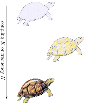
Figure 7: The Zeno subspaces. The Hilbert space of the system splits into sectors (the scutes of the shell of a tortoise) and a dynamical superselection rule appears as the number of measurements/kicks $N$ or the coupling $K$ is increased. This drawing blends the paradox of the sped arrow that never reaches its target with that of the tortoise and swifter-running Achilles, which was also proposed by Zeno in order to counter the idea of motion: in a race in which the tortoise has a head start, Achilles can never overtake it, because before he comes up to the point at which the tortoise started, the tortoise will have got a little way, and so on ad infinitum: “that which is in locomotion must arrive at the half-way stage before it arrives at the goal” [8]. In our quantum context, sped arrows can only move within the scutes, but never cross the boundary between different scutes.

Notice, however, that there is one important difference between the nonunitary evolution discussed in Sec. 13.1 and the dynamical evolutions discussed in Secs. 13.2-13.3: indeed, if the initial state $\rho_{0}$ contains coherent terms between any two Zeno subspaces ${\cal H}_{n}$ and ${\cal H}_{m}$, $P_{n}\rho_{0}P_{m}\neq 0$, these vanish after the first projection (154) in Sec. 13.1: $P_{n}\rho(0^{+})P_{m}=0$ [the state becomes an incoherent superposition $\rho(0^{+})\neq\rho_{0}$, whence $\mathrm{Tr}\rho(0^{+})^{2}<\mathrm{Tr}\rho_{0}^{2}$]. On the other hand, such terms are preserved by the dynamical (unitary) evolutions analyzed in Secs. 13.2-13.3, and do not vanish, even though they wildly oscillate. For example, consider the initial state

$$\rho_{0}=(P_{n}+P_{m})\rho_{0}(P_{n}+P_{m}),\qquad P_{n}\rho_{0}P_{m}\neq 0.$$ (178)

By (165) and (173) it evolves into

$$\rho(t) = U_{\rm Z}^{(n)}(t)\rho_{0}U_{\rm Z}^{(n)\dagger}(t)+U_{\rm Z}^{(m)}(t)\rho_{0}U_{\rm Z}^{(m)}(t)$$ (179)

$$+\;\mathrm{e}^{-iN(\lambda_{n}-\lambda_{m})}U_{\rm Z}^{(n)}(t)\rho_{0}U_{\rm Z}^{(m)\dagger}(t)$$

$$+\;\mathrm{e}^{iN(\lambda_{n}-\lambda_{m})}U_{\rm Z}^{(m)}(t)\rho_{0}U_{\rm Z}^{(n)\dagger}(t)$$

or

$$\rho(t) = U_{\rm Z}^{(n)}(t)\rho_{0}U_{\rm Z}^{(n)\dagger}(t)+U_{\rm Z}^{(m)}(t)\rho_{0}U_{\rm Z}^{(m)}(t)$$ (180)

$$+\;\mathrm{e}^{-iK(\eta_{n}-\eta_{m})t}U_{\rm Z}^{(n)}(t)\rho_{0}U_{\rm Z}^{(m)\dagger}(t)$$

$$+\;\mathrm{e}^{iK(\eta_{n}-\eta_{m})t}U_{\rm Z}^{(m)}(t)\rho_{0}U_{\rm Z}^{(n)\dagger}(t),$$

respectively, at variance with (154). Therefore $\mathrm{Tr}\rho(t)^{2}=\mathrm{Tr}\rho_{0}^{2}$ for any $t$ and the Zeno dynamics is unitary in the whole Hilbert space ${\cal H}$. We notice that these coherent terms become unobservable in the large-$N$ or large-$K$ limit, as a consequence of the Riemann-Lebesgue theorem (applied to any observable that “connects” different sectors and whose time resolution is finite). This interesting aspect is reminiscent of some results on “classical” observables [78], semiclassical limit [15] and quantum measurement theory [163, 6, 102, 103, 7]. It is also interesting to note that the superselection rules discussed here are de facto equivalent to the celebrated “W³” ones [184, 185], but turn out to be a mere consequence of the Zeno dynamics.

13.5 Origin of equivalence between continuous and pulsed formulations

The equivalence between the pulsed and continuous measurement formulation of the quantum Zeno effect can be pushed much further: let us show that the two procedures differ only in the order in which two limits are computed [37]. As we have seen, the continuous case deals with the strong coupling limit

$$H_{K}=H+KH_{\mathrm{c}},\qquad K\rightarrow\infty$$ (181)

and the Zeno subspaces are the eigenspaces of $H_{\mathrm{c}}$. On the other hand, the kicked dynamics entails the limit $N\rightarrow\infty$ in (159) and the Zeno subspaces are the eigenspaces of $U_{\mathrm{kick}}$. This evolution is generated by the Hamiltonian

$$H_{\mathrm{kick}}=H+\tau_{0}H_{\mathrm{c}}\sum_{n}\delta(t-n\tau),\qquad\tau\rightarrow 0$$ (182)

where $\tau$ is the period between two kicks and the unitary evolution during a kick is $U_{\mathrm{kick}}=\exp(-i\tau_{0}H_{\mathrm{kick}})$. The limit $N\rightarrow\infty$ in (159) corresponds to $\tau\rightarrow 0$. The two dynamics (181) and (182) are both limiting cases of the following one

$$H(\tau,K) = H+KH_{\mathrm{kick}}\sum_{n}g\left(\frac{t-n(\tau+\tau_{0}/K)}{\tau_{0}/K}\right),$$ (183)

where the function $g$ has the properties

$$\sum_{n}g(x-n) = 1$$ (184)

$$\lim_{K\rightarrow\infty}Kg(Kx) = \delta(x).$$ (185)

For example we can consider $g(x)=\chi_{[-1/2,1/2]}(x)$. In Eq. (183) the period between two kicks is $\tau_{0}/K+\tau$, while the kick lasts for a time $\tau_{0}/K$. By taking the limit $\tau\rightarrow 0$ in Eq. (183), i.e., a sequence of pulses of finite duration $\tau_{0}/K$ without any idle time among them, and using property (184), one recovers the continuous case (181). Then, by taking the strong coupling limit $K\rightarrow\infty$ one gets the Zeno subspaces. On the other hand, by taking the $K\rightarrow\infty$ limit, i.e., the limit of shorter pulses (but with the same global—integral—effect), and using property (185) and the identity $\delta(t/\tau_{0})=\tau_{0}\delta(t)$, one obtains the kicked case (182). Then, by taking the vanishing idle time limit $\tau\rightarrow 0$ one gets again the Zeno subspaces. In short, the mathematical equivalence between the two approaches is expressed by the relation

$$\lim_{K\rightarrow\infty}\;\lim_{\tau\rightarrow 0}H(\tau,K)=\lim_{\tau\rightarrow 0}\;\lim_{K\rightarrow\infty}H(\tau,K),$$ (186)

(for almost all $\tau_{0}$) with the left (right) side expressing the continuous (pulsed) case. Note that this formal equivalence must physically be checked on a case by case basis, and it is legitimate only if the inverse Zeno regime is avoided and the role of the form factors clearly spelled out. That is, physically the relevant timescales play a crucial role, and in practice there certainly can be a difference [49] between kicked dynamics and continuous coupling, in spite of their equivalence in the above mathematical limit.

14 Examples

One of the main potential applications of the quantum Zeno subspaces concerns the possibility of freezing the loss of quantum mechanical coherence and probability leakage due to the interaction of the system of interest with its environment. Let us therefore look at some elementary examples in the light of the three different formulations of the Zeno effect summarized in Sec. 13. In the following, it can be helpful to think of the Zeno subspace ${\cal H}_{1}$ as the quantum computation subspace (qubit) that one wants to protect from decoherence.

14.1 Von Neumann’s projections

Consider a 3-level system in ${\cal H}_{\mathrm{sys}}=\mathbb{C}^{3}$

$$\left\langle a\right|=(1,0,0),\quad\left\langle b\right|=(0,1,0),\quad\left\langle c\right|=(0,0,1)$$ (187)

and the Hamiltonian

$$H=\Omega_{1}(\left|a\right\rangle\left\langle b\right|+\left|b\right\rangle\left\langle a\right|)+\Omega_{2}(\left|b\right\rangle\left\langle c\right|+\left|c\right\rangle\left\langle b\right|)=\pmatrix{0&\Omega_{1}&0\cr\Omega_{1}&0&\Omega_{2}\cr 0&\Omega_{2}&0}.$$ (188)

We perform the (incomplete, nonselective) projective measurements ($P_{1}+P_{2}=\mathbf{1}$)

$$P_{1}=\left|a\right\rangle\left\langle a\right|+\left|b\right\rangle\left\langle b\right|=\pmatrix{1&0&0\cr 0&1&0\cr 0&0&0},\quad P_{2}=\left|c\right\rangle\left\langle c\right|=\pmatrix{0&0&0\cr 0&0&0\cr 0&0&1},$$ (189)

yielding the partition (143), with $\mathrm{dim}{\cal H}_{1}=2$, $\mathrm{dim}{\cal H}_{2}=1$. The evolution operators (156) read

$$U_{\rm Z}^{(1)}(t) =P_{1}\exp(-iP_{1}HP_{1}t) =P_{1}\exp\left[-i\pmatrix{0&\Omega_{1}t&0\cr\Omega_{1}t&0&0\cr 0&0&0}\right]$$

$$=\pmatrix{\cos\Omega_{1}t&-i\sin\Omega_{1}t&0\cr-i\sin\Omega_{1}t&\cos\Omega_{1}t&0\cr 0&0&0},$$

$$U_{\rm Z}^{(2)}(t) =P_{2}\exp(-iP_{2}HP_{2}t) =P_{2}=\pmatrix{0&0&0\cr 0&0&0\cr 0&0&1}$$ (190)

and the Zeno Hamiltonian (158) is

$$H_{\mathrm{Z}}=P_{1}HP_{1}+P_{2}HP_{2}=\pmatrix{0&\Omega_{1}&0\cr\Omega_{1}&0&0\cr 0&0&0}.$$ (191)

The initial state (146) evolves according to (154): in the Zeno limit ($N\to\infty$), the subspaces ${\cal H}_{1}$ and ${\cal H}_{2}$ decouple. If the coupling $\Omega_{2}$ is viewed as a caricature of the loss of quantum mechanical coherence, the subspace ${\cal H}_{1}$ becomes “decoherence free” [133, 191, 28]. See Fig. 8.

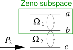
Figure 8: Three level system undergoing measurements ($P_{1}$ not indicated). We explicitly showed the Zeno subspace ${\cal H}_{1}$.

14.2 Kicks

In order to exemplify how unitary kicks yield the Zeno subspaces, consider the 4-level system in the enlarged Hilbert space ${\cal H}_{\mathrm{sys}}\oplus\mathrm{span}\{\left|M\right\rangle\}$

$$\left\langle a\right|=(1,0,0,0),\quad\left\langle b\right|=(0,1,0,0),$$

$$\left\langle c\right|=(0,0,1,0),\quad\left\langle M\right|=(0,0,0,1)$$ (192)

and the Hamiltonian

$$H=\Omega_{1}(\left|a\right\rangle\left\langle b\right|+\left|b\right\rangle\left\langle a\right|)+\Omega_{2}(\left|b\right\rangle\left\langle c\right|+\left|c\right\rangle\left\langle b\right|)=\pmatrix{0&\Omega_{1}&0&0\cr\Omega_{1}&0&\Omega_{2}&0\cr 0&\Omega_{2}&0&0\cr 0&0&0&0}.$$ (193)

This is the same example as (187)-(188), but we added a fourth level $\left|M\right\rangle$. We now couple $\left|M\right\rangle$ to $\left|c\right\rangle$ by performing the unitary kicks

$$U_{\mathrm{kick}} = P_{1}+\mathrm{e}^{-i\lambda(\left|c\right\rangle\left\langle M\right|+\left|M\right\rangle\left\langle c\right|)}=\pmatrix{1&0&0&0\cr 0&1&0&0\cr 0&0&\cos\lambda&-i\sin\lambda\cr 0&0&-i\sin\lambda&\cos\lambda}$$ (194)

$$= \sum_{n=1,\pm}\mathrm{e}^{-i\lambda_{n}}P_{n},$$

where $\lambda=\lambda_{+}=-\lambda_{-}\neq\lambda_{1}=0$ and the subspaces are defined by

$$P_{1} = \left|a\right\rangle\left\langle a\right|+\left|b\right\rangle\left\langle b\right|=\pmatrix{1&0&0&0\cr 0&1&0&0\cr 0&0&0&0\cr 0&0&0&0},$$ (195)

$$P_{\pm} = \frac{(\left|c\right\rangle\pm\left|M\right\rangle)(\left\langle c\right|\pm\left\langle M\right|)}{2}=\frac{1}{2}\pmatrix{0&0&0&0\cr 0&0&0&0\cr 0&0&1&\pm 1\cr 0&0&\pm 1&1}.$$ (196)

($P_{1}+P_{-}+P_{+}=\mathbf{1}$.)

Figure 9: Three level system undergoing frequent unitary kicks that couple one of its levels to an “external” system $M$. We explicitly indicated the Zeno subspace ${\cal H}_{1}$.

In the Zeno limit ($N\to\infty$) the subspaces ${\cal H}_{1}$, ${\cal H}_{+}$ and ${\cal H}_{-}$ decouple due to the wildly oscillating phases O$(N)$. See Fig. 9. The Zeno Hamiltonian (163) reads

$$H_{\mathrm{Z}}=\sum_{n}P_{n}HP_{n}=\pmatrix{0&\Omega_{1}&0&0\cr\Omega_{1}&0&0&0\cr 0&0&0&0\cr 0&0&0&0}$$ (197)

and the evolution (165) is

$$U_{N}(t) \sim \exp\left(-i\sum_{n}N\lambda_{n}P_{n}+P_{n}HP_{n}t\right)$$ (198)

$$= \exp\left[-i\pmatrix{0&\Omega_{1}t&0&0\cr\Omega_{1}t&0&0&0\cr 0&0&0&N\lambda\cr 0&0&N\lambda&0}\right]$$

$$= \pmatrix{\cos\Omega_{1}t&-i\sin\Omega_{1}t&0&0\cr-i\sin\Omega_{1}t&\cos\Omega_{1}t&0&0\cr 0&0&\cos N\lambda&-i\sin N\lambda\cr 0&0&-i\sin N\lambda&\cos N\lambda}.$$

This is the scheme adopted by Itano et al in their experiment [76].

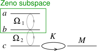
Figure 10: Three level system with one of its levels strongly coupled to an “external” system $M$. We explicitly indicated the Zeno subspace ${\cal H}_{1}$.

14.3 Continuous coupling

Finally, in order to understand how the scheme involving continuous measurements works, add to (193) the Hamiltonian (acting on ${\cal H}_{\mathrm{sys}}\oplus\mathrm{span}\{\left|M\right\rangle\}$)

$$KH_{\mathrm{c}}=K(\left|c\right\rangle\left\langle M\right|+\left|M\right\rangle\left\langle c\right|)=\pmatrix{0&0&0&0\cr 0&0&0&0\cr 0&0&0&K\cr 0&0&K&0}=K\left(P_{+}-P_{-}\right)\;,$$ (199)

where $P_{\pm}$ are the same as in (196). The fourth level $\left|M\right\rangle$ is now continuously coupled to level $\left|c\right\rangle$, $K\in\mathbb{R}$ being the strength of the coupling. As $K$ is increased, level $\left|M\right\rangle$ performs a better “continuous observation” of $\left|c\right\rangle$, yielding the Zeno subspaces. The eigenprojections of $H_{\mathrm{c}}$ [see (172)]

$$H_{\mathrm{c}}=\eta_{1}P_{1}+\eta_{-}P_{-}+\eta_{+}P_{+}$$ (200)

are again (195)-(196), with $\eta_{1}=0,\eta_{\pm}=\pm 1$. Once again, in the Zeno limit ($K\to\infty$) the subspaces ${\cal H}_{1}$, ${\cal H}_{+}$ and ${\cal H}_{-}$ decouple due to the wildly oscillating phases O$(K)$. See Fig. 10. The Zeno Hamiltonian $H_{\mathrm{Z}}$ is given by (171) and turns out to be identical to (197), while the evolution (173) explicitly reads

$$U_{K}(t) \sim \exp\left(-i\sum_{n}Kt\eta_{n}P_{n}+P_{n}HP_{n}t\right)$$ (201)

$$= \exp\left[-i\pmatrix{0&\Omega_{1}t&0&0\cr\Omega_{1}t&0&0&0\cr 0&0&0&Kt\cr 0&0&Kt&0}\right]$$

$$= \pmatrix{\cos\Omega_{1}t&-i\sin\Omega_{1}t&0&0\cr-i\sin\Omega_{1}t&\cos\Omega_{1}t&0&0\cr 0&0&\cos Kt&-i\sin Kt\cr 0&0&-i\sin Kt&\cos Kt}.$$

[Compare with (198): $Kt$ plays the role of $N\lambda$.] This is the scheme adopted by Ketterle and collaborators in their experiment [168].

15 Conclusions and outlook

We analyzed the physical and mathematical aspects of the quantum Zeno dynamics that takes place when one frequently checks whether a quantum system has remained inside a multidimensional Zeno subspace. Unlike in the traditional formulation of the QZE, the system can evolve away from its initial state, although it remains in the eigenspace of the projection operator associated with the measurement.

When the Zeno subspace is finite dimensional, the evolution can be easily (and rigorously) derived. The situation is much more complicated for infinite dimensional projections, such as traditional position measurements, namely projections onto spatial regions. This is an open problem from the mathematical point of view, where the existence of the strong limit of the Zeno product formula remains to be proven. However, if it converges, the Zeno dynamics uniquely determines the boundary conditions, and they turn out to be of Dirichlet type.

The Zeno mechanism not only forces the system to remain in a given subspace, it also constrains its (sub)dynamics in this space, determining the behavior of the wave function on the boundary and yielding a unitary, decoherence free evolution. Besides its theoretical interest, this feature might lead to potential applications and practical implementations of the Zeno constraints in order to tailor subspaces that are robust against decoherence, which are of great interest in quantum information processing applications.

We implicitly assumed, throughout a part of our discussion, the validity of the Copenhagen interpretation, according to which the measurement is considered to be instantaneous. The QZE is traditionally derived by considering a series of rapid, pulsed observations (projections). This became almost a dogma and motivated all seminal experiments. However, a projection operator is a shorthand notation, that summarizes the effects of a much more complicated underlying dynamical process, involving a huge number of elementary quantum mechanical systems. Later formulations emphasized that the QZE can also be generated by pulsed and even continuous Hamiltonian interaction. Here we have shown that all these seemingly different pictures can be unified and in particular the QZE in its continuous-interaction and pulsed (“kicks” or “bang-bang”) formulation can be understood as limits of a single Hamiltonian, Eq. (183), giving rise to either pulsed or continuous dynamics, with a resulting partitioning of the controlled system’s Hilbert space into quantum Zeno subspaces. This unified view not only offers the advantage of conceptual simplicity, but also has significant practical consequences: it shows that the scope of all the methods analyzed here (QZE, kicks and continuous interaction) are wider than previously suspected, leading to greater flexibility in their implementation.

The present work enters an experimentally uncharted area, although the property of being a multidimensional measurement is not at all exotic: the quantum Zeno dynamics has not been experimentally demonstrated, even for a two-dimensional subspace (a qubit). It would be of great interest to verify it for an $N$ level system or for a collection of qubits and in particular for the most basic quantum measurement: position.

References

References

- [1] Altenmüller T P and Schenzle A 1994 Phys. Rev. A 49 2016
- [2] Álvarez G A, Danieli E P, Levstein P R and Pastawski H M 2006 J. Chem. Phys. 124 194507
- [3] Alvarez-Estrada R F and Sánchez-Gómez J L 1999 Phys. Lett. A 253 252
- [4] Anderson W A and Nelson F A 1963 J. Chem. Phys. 39 183
- [5] Antoniou I, Karpov E, Pronko G and Yarevsky E 2001 Phys. Rev. A 63 062110
- [6] Araki H 1962 Einführung in die Axiomatische Quantenfeldtheorie I, II (ETH-Lecture, ETH, Zurich)
- [7] Araki H 1980 Prog. Theor. Phys. 64 719
- [8] Aristotle Physics VI:9, 239b10
- [9] Balzer C, Hannemann T, Reib D, Wunderlich C, Neuhauser W and Toschek P E 2002 Opt. Commun. 211 235
- [10] Balzer C, Huesmann R, Neuhauser W and Toschek P E 2000 Opt. Comm. 180 115
- [11] Beige A, Braun D, Tregenna B and Knight P L 2000 Phys. Rev. Lett. 85 1762
- [12] Beige A and Hegerfeldt G 1996 Phys. Rev. A 53 53
- [13] Bernardini C, Maiani L and Testa M 1993 Phys. Rev. Lett. 71 2687
- [14] Berry M 1995 in: Fundamental Problems in Quantum Theory, eds Greenberger D M and Zeilinger A (Ann. N.Y. Acad. Sci. Vol. 755, New York) p. 303
- [15] Berry M V: ‘Chaos and the semiclassical limit of quantum mechanics (is the moon there when somebody looks?)’. In Quantum Mechanics: Scientific perspectives on divine action (eds: R.J. Russell, P. Clayton, K. Wegter-McNelly and J. Polkinghorne), Vatican Observatory CTNS publications, p. 41
- [16] Berry M V, Balazs N L, Tabor M and Voros A 1979 Ann. Phys. 122 26
- [17] Berry M V and Klein S 1996 J. Mod. Optics 43 165
- [18] Beskow A and Nilsson J 1967 Arkiv für Fysik 34 561
- [19] Blanchard Ph and Jadczyk A 1993, Phys. Lett. A 183 272
- [20] Breit G and Wigner E P 1936 Phys. Rev. 49 519
- [21] Carinena J F, Grabowski J and Marmo G 2000 Int. J. Mod. Phys. A 15 4797
- [22] Casati G, Chirikov B V, Ford J and Izrailev F M 1979: in Stochastic behaviour in classical and quantum Hamiltonian systems, ed. by Casati G, Ford J, Lecture Notes in Physics (Springer-Verlag, Berlin) 93 334
- [23] Chernoff P R T 1974 Product Formulas, Nonlinear Semigroups, and Addition of Unbounded Operators (Memoirs of the American Mathematical Society 140 Providence)
- [24] Cirac J I, Schenzle A and Zoller P 1994 Europhys. Lett. 27 123
- [25] Compagno G, Messina A, Nakazato H, Napoli A, Unoki M and Yuasa K 2004 Phys. Rev. A 70 052316
- [26] Cook R J 1988 Phys. Scr. T 21 49
- [27] Delgado F, Muga J G, and García-Calderón G 2006 Phys. Rev. A 74 062102
- [28] Duan L -M and Guo G -C 1997 Phys. Rev. Lett. 79 1953
- [29] Egusquiza I L and Muga J G 2000 Phys. Rev. A 62 032103
- [30] Ernst R R 1966 J. Chem. Phys. 45 3845
- [31] Exner P 1985 Open Quantum Systems and Feynman Integrals (D. Reidel Publishing Company, Dordrecht, Holland)
- [32] Exner P and Ichinose T 2005 Ann. H. Poincaré 6 195
- [33] Exner P, Ichinose T, Neidhardt H and Zagrebnov V 2007 Integral Equations and Operator Theory 57 67
- [34] Facchi P, Gorini V, Marmo G, Pascazio S and Sudarshan E C G 2000 Phys. Lett. A 275 12
- [35] Facchi P, Hradil Z, Krenn G, Pascazio S and Rehacek J 2002 Phys. Rev. A 66 012110
- [36] Facchi P, Klein A G, Pascazio S and Schulman L S 1999 Phys. Lett. A 257 232
- [37] Facchi P, Lidar D A and Pascazio S 2004 Phys. Rev. A 69 032314
- [38] Facchi P, Marmo G, Pascazio S, Scardicchio A and Sudarshan E C G 2004 J. Opt. B: Quantum Semicl. Optics 6 S492
- [39] Facchi P, Nakazato H and Pascazio S 2001 Phys. Rev. Lett. 86 2699
- [40] Facchi P, Nakazato H, Pascazio S, Peřina J and Řeháček J 2001, Phys. Lett. A 279 117
- [41] Facchi P and Pascazio S 1998 Phys. Lett. A 241 139
- [42] Facchi P and Pascazio S 1999 Physica A 271 133
- [43] Facchi P and Pascazio S 2000 Phys. Rev. A62 023804
- [44] Facchi P and Pascazio S 2001 Progress in Optics 42 147
- [45] Facchi P and Pascazio S 2002 Phys. Rev. Lett. 89 080401
- [46] Facchi P and Pascazio S 2003 Three different manifestations of the quantum Zeno effect, in Irreversible Quantum Dynamics, edited by F. Benatti and R. Floreanini, Lecture Notes in Physics (Springer-Verlag, Berlin) Vol. 622 141
- [47] Facchi P, Pascazio S and Scardicchio A 1999 Phys. Rev. Lett. 83 61
- [48] Facchi P, Pascazio S, Scardicchio A and Schulman L S 2001 Phys. Rev. A 65 012108
- [49] Facchi P, Tasaki S, Pascazio S, Nakazato H, Tokuse A and Lidar D A 2005 Phys. Rev. A 71 022302
- [50] Fermi E 1932 Rev. Mod. Phys. 4 87
- [51] Fermi E 1950 Nuclear Physics (University of Chicago, Chicago) pp. 136, 148
- [52] Fermi E 1960 Notes on Quantum Mechanics. A Course Given at the University of Chicago in 1954 edited by E Segré (University of Chicago, Chicago) Lec. 23
- [53] Fischer M C, Gutiérrez-Medina B and Raizen M G 2001 Phys. Rev. Lett. 87 040402
- [54] Fock V and N. Krylov N 1947 J. Phys. 11 112
- [55] Franson J D , Jacobs B C and Pittman T B 2004 Phys. Rev. A 70 062302
- [56] Freeman R, Kempsell S P and Levitt M H 1979 J. Magn. Reson. 35 447
- [57] Frerichs V and Schenzle A 1992 in: Foundations of Quantum Mechanics, eds T.D. Black, M.M. Nieto, H.S. Pilloff, M.O. Scully and R.M. Sinclair (World Scientific, Singapore)
- [58] Friedman C N 1972 Indiana Univ. Math. J. 21 1001
- [59] Friedman C N 1976 Ann. Phys. 98 87
- [60] Froese R and Herbst I 2001 Commun. Math. Phys. 220 489 and references therein
- [61] Gamow G 1928 Z. Phys. 51 204
- [62] Gordon G, Erez N and Kurizki G 2007 J. Phys. B: At. Mol. Opt. Phys. 40 S75
- [63] Gustafson K 1983: “Irreversibility questions in chemistry, quantum-counting, and time-delay” in Energy storage and redistribution in molecules ed. by Hinze J (Plenum), and refs. [10,12] therein
- [64] Gustafson K 2002 “A Zeno story” quant-ph/0203032
- [65] Gustafson K and Misra B 1976 Lett. Math. Phys. 1 275
- [66] Hardy G H 1940 A mathematician’s apology (Cambridge University Press)
- [67] Harris R A and Stodolsky L 1982 Phys. Lett. B 116 464
- [68] Hellund E J 1953 Phys. Rev. 89 919
- [69] Hille E and Phillips R S 1957 Functional analysis and semigroups (Am. Math. Soc. Colloq. Publ. Vol. 31)
- [70] Home D and Whitaker M A B 1997 Ann. Phys. 258 237
- [71] Home D and Whitaker M A B 1998 Phys. Lett. A 239 6
- [72] Hosten O, Rakher M T, Barreiro J T, Peters N A and Kwiat G R 2006 Nature 439 949
- [73] Hradil Z, Nakazato H, Namiki M, Pascazio S and Rauch H 1998 Phys. Lett. A 239 333
- [74] Huang H, Zhu S -Y, Zubairy M S and Scully M O 1996 Phys. Rev. A 53 1834
- [75] Inagaki S, Namiki M and Tajiri T 1992 Phys. Lett. A 166 5
- [76] Itano W M, Heinzen D J, Bollinger JJ and Wineland D J 1990 Phys. Rev. A 41 2295
- [77] Itano W M, Heinzen D J, Bollinger JJ and Wineland D J 1991 Phys. Rev. A 43 5168
- [78] Jauch J M 1964 Helv. Phys. Acta 37 293
- [79] Jericha E, Schwab D E, Jäkel M R, Carlile C J and Rauch H 2000 Physica B 283 414
- [80] Johansson G private communication
- [81] Joichi I, Matsumoto Sh and Yoshimura M 1998 Phys. Rev. D 58 045004
- [82] Kato T 1978 Trotter’s product formula for arbitrary pair of self-adjoint contraction semigroups Topics in functional analysis, Adv. in Math. Suppl. Stud. 3 (Academic Press, New York)
- [83] Kato T 1980 Perturbation Theory for Linear Operators (Springer, Berlin)
- [84] Kaulakys B and V Gontis 1997 Phys. Rev. A 56 1131
- [85] Khalfin L A 1957 Dokl. Acad. Nauk USSR 115 277 [1957 Sov. Phys. Dokl. 2 340]
- [86] Khalfin L A 1958 Zh. Eksp. Teor. Fiz. 33 1371 [1958 Sov. Phys. JET 6 1053]
- [87] Khalfin L A 1968 Zh. Eksp. Teor. Fiz. Pis. Red. 8 106 [1968 JETP Letters 8 65]
- [88] Kofman A G and Kurizki G 1996 Phys. Rev. A 54 R3750
- [89] Kofman A G and Kurizki G 1999 Acta Physica Slovaca 49 541
- [90] Kofman A G and Kurizki G 2000 Nature 405 546
- [91] Koshino K and Shimizu A 2005 Phys. Rep. 412 191
- [92] Kraus K 1981 Found. Phys. 11 547
- [93] Kwiat R, Weinfurter H, Herzog T, Zeilinger A, and Kasevich M 1995 Phys. Rev. Lett. 74 4763
- [94] Lane A M 1983 Phys. Lett. A 99 359
- [95] Levitt M H, Freeman R and Frenkiel T A 1982 J. Magn. Reson. 47 328
- [96] Lidar D A and Whaley K B 2003 “Decoherence-Free Subspaces and Subsystems” in Irreversible Quantum Dynamics Benatti F and Floreanini R Eds. 622 83 (Springer Lecture Notes in Physics Berlin)
- [97] Longhi S 2006 Phys. Rev. Lett. 97 110402
- [98] Lüders G 1951 Ann. Phys. (Leipzig) 8 322
- [99] Luis A 2001 Phys. Rev. A 64 032104
- [100] Luis A and Sánchez–Soto L L 1998 Phys. Rev. A 57 781
- [101] Luis A and Periňa J 1996 Phys. Rev. Lett. 76 4340
- [102] Machida S and , Namiki M 1980 Prog. Theor. Phys. 63 1457
- [103] Machida S and , Namiki M 1980 Prog. Theor. Phys. 63 1833
- [104] Maiani L and Testa M 1998 Ann. Phys. (NY) 263 353
- [105] Mandel L and Wolf E 1995 Optical coherence and quantum optics (Cambridge University Press, Cambridge)
- [106] Mandelstam L and Tamm I 1945 J. Phys. 9 249
- [107] Maniscalco S, Piilo J and Suominen K-A 2006 Phys. Rev. Lett. 97 130402
- [108] Maniscalco S, Francica F, Zaffino R L, Lo Gullo N and Plastina F 2008 Phys. Rev. Lett. 100 090503
- [109] Man’ko V I, Marmo G, Zaccaria F and Sudarshan E C G 1997 Int. J. Mod. Phys. B 11 1281
- [110] Matolcsi M and Shvidkoy R 2003 Arch. Math. 81 309
- [111] Miglietta F, Rimini A 1984 Phys. Lett. B 139 353
- [112] Mihokova E, Pascazio S and Schulman L S 1997 Phys. Rev. A 56 25
- [113] Militello B and Messina A 2004 Phys. Rev. A 70 033408
- [114] Militello M, Messina A and Napoli A 2001 Phys. Lett. A 286 369
- [115] Militello B, Messina A and Napoli A 2001 Fortschr. Phys. 49 1041
- [116] Militello B, Yuasa K, Nakazato H and Messina A 2007 Phys. Rev. A 76 042110
- [117] Misra B and Sudarshan E C G 1977 J. Math. Phys. 18 756
- [118] Mølhave K and Drewsen M 2000 Phys. Lett. A 268 45
- [119] Muga J G, Delgado F, del Campo A and García-Calderón G 2006 Phys. Rev. A 73 052112
- [120] Muga J G and Leavens C R 2000 Phys. Rept. 338 353
- [121] Muga J G, Wei G W and Snider R F 1996 Europhys. Lett. 35 247
- [122] Nagels B, Hermans L J F and Chapovsky P L 1997 Phys. Rev. Lett. 79 3097
- [123] Nakanishi T, Yamane K and Kitano M 2001 Phys. Rev. A 65 013404
- [124] Nakazato H, Namiki M and Pascazio S 1996 Int. J. Mod. Phys. B 10 247
- [125] Nakazato H, Namiki M, Pascazio S and Rauch H 1995 Phys. Lett. A 199 27
- [126] Nakazato H, Namiki M, Pascazio S and Rauch H 1996 Phys. Lett. A 217 203
- [127] Nakazato H, Takazawa T and Yuasa K 2003 Phys. Rev. Lett. 90 060401
- [128] Nakazato H, Unoki M and Yuasa K 2004 Phys. Rev. A 70 012303
- [129] Nakazato H, Yuasa K, Militello B and Messina A 2008 Phys. Rev. A 77 042114
- [130] Namiki M and Mugibayashi N 1953 Prog. Theor. Phys. 10 474
- [131] Namiki M, Pascazio S and Nakazato H 1997 Decoherence and Quantum Measurements (World Scientific, Singapore)
- [132] Nelson E 1969 Topics in Dynamics I: Flows, Mathematica Notes (Princeton: Princeton University Press) p 114
- [133] Palma G M, Suominen K A and Ekert A K 1996 Proc. Roy. Soc. London Ser. A 452 567
- [134] Panov A D Phys. Lett. A 260 441
- [135] Pascazio S 1996 “Quantum Zeno effect and inverse Zeno effect” in Quantum Interferometry eds De Martini F, Denardo G and Shih Y (VCH, Weinheim) p. 525
- [136] Pascazio S 1997 Found. Phys. 27 1655
- [137] Pascazio S and Facchi P 1999 Acta Physica Slovaca 49 557
- [138] Pascazio S and Namiki M 1994 Phys. Rev. A 50 4582
- [139] Pascazio S, Namiki M, Badurek G and Rauch H 1993 Phys. Lett. A 179 155
- [140] Paternostro M and Kim M S 2005 New J. Phys. 7 43
- [141] Pati A 1996 Phys. Lett. A 215 7
- [142] Peres A 1980 Am. J. Phys. 48 931
- [143] Peres A 2002 Quantum Theory: Concepts and Methods (Kluwer Academic Publisher, New York)
- [144] Peres A and Ron A 1990 Phys. Rev. A 42 5720
- [145] Petrosky T, Tasaki S and Prigogine I 1990 Phys. Lett. A 151 109
- [146] Petrosky T, Tasaki S and Prigogine I 1991 Physica A 170 306
- [147] Plenio M B, Knight P L and Thompson R C 1996 Opt. Comm. 123 278
- [148] Rauch H 2001 Physica B 297 299
- [149] Reed M and Simon B 1980 Functional Analysis (Academic Press, San Diego)
- [150] Řeháček J, Peřina J, Facchi P, Pascazio S and Mišta L 2000 Phys. Rev. A 62 013804
- [151] Russell B 1945 A history of Western philosophy (Taylor & Francis Books)
- [152] Russell B 1996 The Principles of Mathematics (W W Norton Company)
- [153] Sakurai J J 1994 Modern Quantum Mechanics (Addison Wesley)
- [154] Sasaki M, Hasegawa A, Ishi-Hayase J, Mitsumori Y and Minami F 2005 Phys. Rev. B 71 165314
- [155] Schieve W C, Horwitz L P and Levitan J 1989 Phys. Lett. A 136 264
- [156] Schiller C 2007 Motion Mountain – The Adventure of Physics (available on-line at www.motionmountain.net)
- [157] Schmidt A U 2002 J. Phys. A 35 7817
- [158] Schmidt A U 2003 J. Phys. A 36 1135
- [159] Schmidt A U 2004 Mathematical Physics Research on the Leading Edge ed C V Benton (Hauppauge NY: Nova Science) pp 113-43
- [160] Schulman L S 1997 J. Phys. A 30 L293
- [161] Schulman L S 1998 Phys. Rev. A 57 1509
- [162] Schulman L S, Ranfagni A and Mugnai D 1994 Phys. Scr. 49 536
- [163] Schwinger J 1959 Proc. Nat. Acad. Sc. 45 1552; reproduced in Schwinger J 1991 Quantum kinematics and dynamics (Perseus Publishing, New York) p. 26
- [164] Seke J 1994 Physica A 203 269
- [165] Seke J 1994 Physica A 203 284
- [166] Simonius M 1978 Phys. Rev. Lett. 40 980
- [167] Sokal A and Bricmont J 1998 Fashionable Nonsense (Picador)
- [168] Streed E W, Mun J, Boyd M, Campbell G K, Medley P, Ketterle W and Pritchard D E 2006 Phys. Rev. Lett. 97 260402
- [169] Sudbery A 1984 Ann. Phys. 157 512
- [170] Thun K and Peřina J 1998 Phys. Lett. A 249 363
- [171] Tian L 2007 Phys. Rev. Lett. 98 153602
- [172] Toschek P E and Wunderlich C 2001 Eur. Phys. J. D 14 387
- [173] Trotter H F 1958 Pacific J. Math. 8 887
- [174] Trotter H F 1959 Proc. Am. Math. Soc. 10 545
- [175] Valanju P, Sudarshan E C G and Chiu C B 1980 Phys. Rev. D 21 1304
- [176] Venugopalan A and Ghosh R 1995 Phys. Lett. A 204 11
- [177] Viola L and Lloyd S 1998 Phys. Rev. A 58 2733
- [178] Vion D private communication.
- [179] von Neumann J 1932 Die Mathematische Grundlagen der Quantenmechanik (Springer, Berlin) [English translation by E. T. Beyer E T 1955 Mathematical Foundation of Quantum Mechanics (Princeton University Press, Princeton)]. For the QZE, see in particular p. 195 of the German edition (p. 366 of the English translation).
- [180] Weinberg S 1996 The New York Review of Books Volume XLIII No. 13, pp 11-15
- [181] Weisskopf V and Wigner E P 1930 Z. Phys. 63 54
- [182] Weisskopf V and Wigner E P 1930 Z. Phys. 65 18
- [183] Whitaker M A B 2000 Progr. Q. Electr. 24 1
- [184] Wick G C, Wightman A S and Wigner E P 1952 Phys. Rev. 88 101
- [185] Wick G C, Wightman A S and Wigner E P 1970 Phys. Rev. D 1 3267
- [186] Wilkinson S R, Bharucha C F, Fischer M C, Madison K W, Morrow P R, Niu Q, Sundaram B and Raizen M G 1997 Nature 387 575
- [187] Wu L A, Lidar D A and Schneider S 2004 Phys. Rev. A 70 032322
- [188] Wunderlich C, Balzer C and Toschek P E 2001 Z. Naturforsch. 56a 160
- [189] Xiao L and Jones J A 2006 Physics Letters A 359 424
- [190] Yuasa K and Nakazato H 2005 Prog. Theor. Phys. 114 523
- [191] Zanardi P and Rasetti M 1997 Phys. Rev. Lett. 79 3306
- [192] Zhu C and Klauder J R 1993 Am. J. Phys. 61 605
- [193] Zhu S -Y, Narducci L M and Scully M O 1995 Phys. Rev. A 52 4791
- [194] Zhu S -Y and Scully M O 1996 Phys. Rev. Lett. 76 388