On Oligopoly Spectrum Allocation Game in Cognitive Radio Networks with Capacity Constraints

Abstract

Dynamic spectrum sharing is a promising technology to improve spectrum utilization in the future wireless networks. The flexible spectrum management provides new opportunities for licensed primary user and unlicensed secondary users to reallocate the spectrum resource efficiently. In this paper, we present an oligopoly pricing framework for dynamic spectrum allocation in which the primary users sell excessive spectrum to the secondary users for monetary return. We present two approaches, the strict constraints (type-I) and the QoS penalty (type-II), to model the realistic situation that the primary users have limited capacities. In the oligopoly model with strict constraints, we propose a low-complexity searching method to obtain the Nash Equilibrium and prove its uniqueness. When reduced to a duopoly game, we analytically show the interesting gaps in the leader-follower pricing strategy. In the QoS penalty based oligopoly model, a novel variable transformation method is developed to derive the unique Nash Equilibrium. When the market information is limited, we provide three myopically optimal algorithms “StrictBEST”, “StrictBR” and “QoSBEST” that enable price adjustment for duopoly primary users based on the Best Response Function (BRF) and the bounded rationality (BR) principles. Numerical results validate the effectiveness of our analysis and demonstrate the fast convergence of “StrictBEST” as well as “QoSBEST” to the Nash Equilibrium. For the “StrictBR” algorithm, we reveal the chaotic behaviors of dynamic price adaptation in response to the learning rates.

center

1 Introduction

Wireless spectrum has become the scarcest resource due to the dramatic development of mobile telecommunication industry in the last decades. However, recent studies by the Federal Communications Commission (FCC) show that traditional fixed allocation policy results in very low efficiency in radio spectrum utilization. The increasing spectrum demand, together with the resource scarcity, gives rise to the development of cognitive radio networks that enable dynamic spectrum access. Within a dynamic spectrum access system, radio spectrum resources are allocated by agile management schemes in terms of spectrum market among the unlicensed (i.e., secondary) users and the licensed (i.e., primary) users [3]. When the possessed spectrum is not fully utilized, a primary user has an opportunity to sell the excessive spectrum to the secondary users for monetary payoff. This is also referred to as spectrum trading mechanism in [2] which involves spectrum selling and purchasing processes. Therefore, it is natural to consider the spectrum allocation in the perspective of economic models and market strategies.

In such an emerging network scenario, multiple primary users coexist in the same geographical site and compete for the access or the purchase of secondary users equipped with cognitive radios. Hence, an important problem for the spectrum trading is how the primary users set prices of per-unit spectrum in a competitive market. For example, if a primary user sets a very low price, it might result in the loss of revenue (or profit). On the contrary, if the price is set too expensive, the secondary users are inclined to purchase from other spectrum holders. Niyato et.al [2] initially introduce the oligopoly pricing theory to characterize the interactions between the spectrum abundant side (primary users) and the demanding side (secondary users). In the oligopoly spectrum market, a commonly used quadratic utility is adopted to quantify the spectrum demand of the secondary service, and each primary user aims to maximize the individual profit. In [3], Jia and Zhang study the competitions and dynamics of spectrum allocation in a duopoly market via a non-cooperative two-stage game. However, authors in [2] do not consider an important feature that a primary user usually has limited capacity to lease. Authors in [3] mainly focus on the situation that both two wireless service providers have limited spectrum capacities in the price competition stage. In fact, the price competition in a more general oligopoly game is rather difficult to be analyzed when the constraints of spectrum capacity are incorporated.

In this paper, we investigate the competitive pricing of a general oligopoly spectrum game. Distinguished from previous work, our study concentrates on the capacity-constrained pricing that is quite common to the primary users. To characterize the limitation in leasing spectrum resource, we employ two approaches: the strict constraints (type-I) and the QoS penalty functions (type-II). In the market model with type-I constraints, each primary user has a certain spectrum bound so that it might not be able to provide the best spectrum demand. We address the following challenging issues: a) is there a unique Nash Equilibrium (NE) in such a capacity-constrained spectrum game? b) if YES, how to find the NE efficiently? c) especially in duopoly games, what are the impacts of capacity constrains on the NEs and the system dynamics? In the type-II market model, the capacity constraint of a primary user is absorbed in the utility as a barrier penalty function. This corresponds to the scenario that the leased spectrum is transferred from the existing services of primary users. They offer spectrum for monetary return, however, at the cost of QoS decrease of primary services. Here, we model the QoS of a primary service as a function of the queueing delay. Generally, explicit solution does not exist in such an oligopoly spectrum allocation game. We present a novel method to discover the NE and to prove its uniqueness. Consider the fact that a primary user usually has no knowledge of the utilities and the price-demand functions of its opponents, we develop a set of price adjustment algorithms based on the best response dynamics and the bounded rationality principles.

To summarize, our contributions are:

• We formulate two oligopoly market models to characterize the capacity limitations: the strict constraints (type-I) and the QoS based penalty functions (type-II). Given the above market models, the primary users compete for revenue or utility maximization by deciding the prices of per-unit spectrum.

• In the type-I model, we propose a novel searching method to find a Nash Equilibrium and prove its uniqueness. Interestingly, we find the revenue gaps in the duopoly Stackelberg game with type-I constraints.

• We present two algorithms, StrictBEST and StrictBR, to adjust prices dynamically based on the best response dynamics and the bounded rationality when the market information is limited.

• In the type-II model, we present an interesting variable transformation method to derive the Nash Equilibrium and prove its uniqueness. The QoSBEST algorithm is proposed to perform spectrum pricing based on the best response dynamics.

• We demonstrate the nonlinear dynamic behaviors in the StrictBR algorithm when the learning rates vary.

The rest of this paper is organized as follows. In section 2, we present the system models of capacity-constrained spectrum market. In section 3 and 4, we analyze the NEs of the noncooperative oligopoly market with type-I and type-II constrains respectively. Section 5 evaluates the analysis and performance of proposed schemes. We present an overview of related work in section 6 and conclude in section 7.

2 System Model

In this section, we present mathematical models to characterize the dynamic spectrum allocation in cognitive radio networks. To capture the realistic spectrum market, two types of capacity constraints are incorporated.

2.1 Agile Spectrum Market

We consider the cognitive radio network where multiple primary users (PUs) or wireless service providers (WSPs) compete for a shared pool of secondary users. The secondary users are the static/mobile devices equipped with cognitive radio technologies. The primary users are the infrastructure based wireless operators or the licensed spectrum holders. They are usually treated as the spectrum brokers that lease the unused frequency to the secondary users for monetary payoff. We show the structure of a spectrum market in Fig.1 with a number of primary users and the common secondary users. In this spectrum market, the demands of secondary users depend on the prices of per-unit spectrum. Each primary user chooses its own price to compete for the secondary users’ subscription.

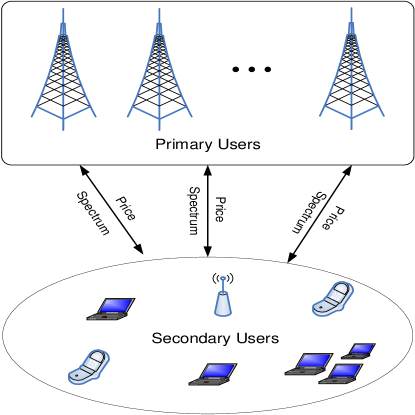
Figure 1: Spectrum Market Structure

2.2 Secondary Users

We characterize the spectrum demands of secondary users in the oligopoly market. Define $\mathcal{N}=\{1,2,\cdots,N\}$ as the set of primary users. Let $p_{i}$ be the price of the $i^{th}$ primary user. Denote $q_{i}$ to be the quantity of spectrum that secondary users buy from the $i^{th}$ primary user. We define the utility of an average secondary user as a quadratic and concave function [1][2]:

$$u(\mathbf{q})=\sum_{i=1}^{N}\alpha_{i}q_{i}-\frac{1}{2}\big{(}\sum_{i=1}^{N}\beta_{i}q_{i}^{2}+2\mu\sum_{i=1}^{N}\sum_{j\neq i}q_{i}q_{j}\big{)}-\sum_{i=1}^{N}p_{i}q_{i},$$ (1)

where $\alpha_{i}$, $\beta_{i}$ are positive constants for all $i\in\mathcal{N}$. Here, $\alpha_{i}$ denotes the spectral efficiency of wireless transmission by a secondary user using the frequency owned by the $i^{th}$ primary user [2]. The spectral efficiencies of primary users can be the same, or different, depending on their center frequencies. For instance, if the center frequency of the $i^{th}$ primary user is high, secondary users may experience large path loss (or low spectral efficiency equivalently) when purchasing spectrum from this primary user. Similar to previous work, we also take the spectrum substitutability into account via the parameter $\mu$. If $\mu$ is 0, a secondary user cannot switch among the primary users. When $0<\mu<\beta_{i}$, a secondary user can switch among the primary users depending on the spectral efficiency and the price of per-unit spectrum. For example, if one primary user increases its price of per-unit of spectrum, some of the secondary users may buy spectrum from other primary users, and vice versa. When $\alpha_{i}=\alpha$ and $\beta_{i}=\mu$ for all $i\in\mathcal{N}$, the spectra of primary users are perfectly substitutive for secondary users. Taking the first-order derivative of the utility function with respect to $q_{i}$ and letting it be 0, we obtain the purchase price of secondary users from the $i^{th}$ primary user:

$$p_{i}=\alpha_{i}-\beta_{i}q_{i}-\mu\sum_{j\neq i}q_{j},\;\;\;\forall i,j\in\mathcal{N}.$$ (2)

The concave function in Eqn.(1) characterizes user satisfaction in terms of the purchased spectrum. In order to guarantee the concavity of utility function, its Jacobian matrix should be negative definite, that is,

$$\frac{\partial u(\mathbf{q})}{\partial\mathbf{q}}=-\mathbf{T}=-\left[\begin{array}[]{cccc}\beta_{1}&\mu&\ldots&\mu\\ \mu&\beta_{2}&\ldots&\mu\\ \vdots&\vdots&\ddots&\vdots\\ \mu&\mu&\ldots&\beta_{N}\end{array}\right]<0,$$ (7)

where $\mathbf{T}$ denotes the above matrix. Note that the concavity of utility function is equivalent to the positive definiteness of $\mathbf{T}$. Here, we present a necessary condition in Lemma 1 to set market parameters.

Lemma 1

The matrix $\mathbf{T}$ is positive definite if the market parameters has $\beta_{i}>\mu>0$ for all $i\in\mathcal{N}$.

Proof: Please refer to the Appendix.  

For the primary users, their strategies are to set prices of per-unit spectrum in the oligopoly market. Thus, the demand function can be expressed as the following:

$$\mathbf{q}=\left[\begin{array}[]{cccc}\beta_{1}&\mu&\ldots&\mu\\ \mu&\beta_{2}&\ldots&\mu\\ \vdots&\vdots&\ddots&\vdots\\ \mu&\mu&\ldots&\beta_{N}\end{array}\right]^{-1}\cdot\left(\left[\begin{array}[]{c}\alpha_{1}\\ \alpha_{2}\\ \vdots\\ \alpha_{N}\end{array}\right]-\mathbf{p}\right)\;$$ (16)

where $\mathbf{p}$ is the price vector and $\mathbf{q}$ is the spectrum demand vector. Given the price vector, the spectrum demand of primary user $i$ is rewritten by:

$$q_{i}=f_{i}(\mathbf{p})=a_{i}-b_{i}p_{i}+\sum_{j\neq i}c_{ij}p_{j},\;\;\;\forall i,j\in\mathcal{N},$$ (17)

where $b_{i}$ as well as $c_{ij}$ are variables computed through Eqn.(16) and $a_{i}=\alpha_{i}b_{i}-\sum_{j\neq i}c_{ij}\alpha_{j}$. Especially, $c_{ij}=c_{ji}$ and $c_{ii}=-b_{i}$ due to the symmetry of convert matrix. The market parameters transformed from Eqn.(16) satisfy the following property,

Lemma 2

The parameters that characterize demand-price function in Eqn.(17), i.e.$\;b_{i}$ and $c_{ij}$ $(i\neq j)$, are positive, given the conditions $\beta_{i}>\mu>0$ for all $i,j\in\mathcal{N}$.

Proof: Please refer to the Appendix.  

In the market model, if the spectral efficiencies (i.e. $\alpha_{i},\forall i\in\mathcal{N}$) are close to each other, one can guarantee the positivity of $a_{i}$ by choosing $\beta_{i}$ and $\mu$ appropriately. We give an example of spectrum market with only two primary users. The utility function results in linear inverse demand functions

$$p_{1} = \alpha_{1}-\beta_{1}q_{1}-\mu q_{2},$$ (18)

$$p_{2} = \alpha_{2}-\beta_{2}q_{2}-\mu q_{1}.$$ (19)

The relationship between prices and demands can be represented by an alternative form:

$$q_{1} = f_{1}(\mathbf{p})=a_{1}-b_{1}p_{1}+cp_{2},$$ (20)

$$q_{2} = f_{2}(\mathbf{p})=a_{2}-b_{2}p_{2}+cp_{1}.$$ (21)

According to Eqn.(16), $a_{i}$ and $b_{i}$ are calculated by: $a_{i}=(\alpha_{i}\beta_{j}-\alpha_{j}\mu)/(\beta_{1}\beta_{2}-\mu^{2})$, $b_{i}=\beta_{j}/(\beta_{1}\beta_{2}-\mu^{2})$ and $c=\mu/(\beta_{1}\beta_{2}-\mu^{2})$ for $i\neq j,(i,j\in\{1,2\})$. To ensure the positivity of prices and demands, there have $\beta_{1}\beta_{2}>\mu^{2}$ and $\alpha_{i}\beta_{j}>\alpha_{j}\mu$ for $i,j=1$ or $2$.

2.3 Primary Users and Bertrand Game Model

The spectra leased by primary users are either unused or transferred from existing applications. The revenue of the $i^{th}$ primary user is a product of the leased spectrum $q_{i}$ and the price $p_{i}$. In practical cognitive radio networks, the primary users cannot always satisfy the demands of the spectrum market. Hence, capacity constraints should be taken into consideration when the primary users set the prices. In this paper, we formulate the oligopoly price competition as a Bertrand game. The players are the primary users, and the strategy of a primary user is the price of unit spectrum. Denote $\pi_{i}$ to be the payoff (or utility) of the primary user $i$ that could be either the revenue or the profit. Let $W_{i}$ be the spectrum size of the $i^{th}$ primary user and $B_{i}$ be the traffic loads of primary services. The spectrum efficiency, $r_{i}^{(p)}$, is defined as the transmission rate per-unit spectrum for the $i^{th}$ primary service. The available spectrum for sale at player $i$ is expressed as $q_{i}^{a}=W_{i}-B_{i}/r_{i}^{(p)}$. We incorporate the capacity constraints into the primary users’ payoff via two approaches:

• Type-I Strict Capacity Constraints: The primary users aim to maximize their monetary revenues under the constraints of capacities. The local optimization model of the $i^{th}$ primary user is expressed as:

  maximize $$\pi_{i}(p_{i},\mathbf{p}_{-i})=p_{i}\cdot\min\{f_{i}(\mathbf{p}),q_{i}^{a}\},$$ (22)

  subject to $$p_{i}>0,\;\;\;\forall i\in\mathcal{N},$$ (23)

  where $\mathbf{p}_{-i}$ is the price vector excluding $p_{i}$.

• Type-II QoS Penalty Functions: An alternative approach is to translate the capacity constraints as the barrier penalty functions to the revenues. Assume that the traffic pattern of a primary user is an i.d.d. poisson arrival process. The average queuing delay of a packet can be approximated by $\frac{B_{i}}{r_{i}^{p}(W_{i}-q_{i})-B_{i}}$, which is adopted to reflect the quality of primary services. Therefore, the utility maximization of a primary user can be expressed as:

  maximize $$\pi_{i}(p_{i},\mathbf{p}_{-i})=p_{i}\min\{f_{i}(\mathbf{p}),q_{i}^{a}\}-\theta\log\frac{B_{i}/r_{i}^{(p)}}{q_{i}^{a}-\min\{f_{i}(\mathbf{p}),q_{i}^{a}\}}$$ (24)

  subject to $$p_{i}>0,\;\;\;\forall i\in\mathcal{N},$$ (25)

  where the positive variable $\theta$ is the weight of the lognormal M/M/1 queuing delay.

Note that the capacity constraints in type-II have different implication from that in type-I. There might have multiple equilibrium points in the type-II model. Therefore, the infeasible solutions are excluded if they are outside of the capacity bounds. In the Bertrand game, the Nash Equilibrium is a vector of spectrum prices that no player can increase its payoff by changing its price unilaterally.

3 Noncooperative Game with Type-I Capacity Constraints

In this section, we first present the static game and the leader-follower game with Type-I capacity constraints, by assuming the availability of full market information of primary users. Furthermore, a dynamic game is formulated to characterize the interactions of price competition when such information is not available.

3.1 Static Duopoly Game

We commence the analysis by considering a duopoly spectrum market with two primary users, and then extend to a more general scenario. In the duopoly game, the NE price of a player is obtained by assuming that the other player also chooses the best strategy. However, the “best” strategies of primary users are different in situations whether the spectrum capacities are sufficient or not. Since there are two primary users, the competitive pricing can be subdivided into four cases. Very recently, authors have analyzed the static games of these four cases and proved the existence of NE in [3]. Their analysis is based on graphical interpretation, which might be difficult to extend to a more general oligopoly game. Inspired by their work, we adopt a slightly different way to study the existence of NE in this section. In comparison with [3], the only difference is the simplicity of analysis in this subsection. Later on, our method will be extended to prove the existence of unique NE in a spectrum game with more than two primary users.

For the $i^{th}$ primary user, it decides the price $p_{i}$ so as to maximize its revenue [3]

$$\max\;\;p_{i}\cdot\min\{q_{i}^{a},a_{i}-b_{i}p_{i}+cp_{j}\},\;\;\forall i,j\in\{1,2\}.$$ (26)

We first investigate the Nash Equilibrium when the available spectra are sufficient for both primary users (PUs). The revenues of PU1 and PU2 can be written as:

$$\pi_{1}(\mathbf{p})=-b_{1}(p_{1}-\frac{a_{1}+cp_{2}}{2b_{1}})^{2}+\frac{(a_{1}+cp_{2})^{2}}{4b_{1}},$$ (27)

$$\pi_{2}(\mathbf{p})=-b_{2}(p_{2}-\frac{a_{2}+cp_{1}}{2b_{2}})^{2}+\frac{(a_{2}+cp_{1})^{2}}{4b_{2}}.$$ (28)

The best responses of PU1 and PU2 are:

$$p_{1}^{*}=\frac{cp_{2}^{*}+a_{1}}{2b_{1}},\;\;\;p_{2}^{*}=\frac{cp_{1}^{*}+a_{2}}{2b_{2}}.$$ (29)

Thus, the duopoly prices at the unique NE are:

$$p_{1}^{*}=\frac{2a_{1}b_{2}+a_{2}c}{4b_{1}b_{2}-c^{2}},\;\;\;p_{2}^{*}=\frac{2a_{2}b_{1}+a_{1}c}{4b_{1}b_{2}-c^{2}}.$$ (30)

The spectrum demands at the unique NE can be expressed by:

$$q_{1}^{*}=\frac{2a_{1}b_{1}b_{2}+b_{1}a_{2}c}{4b_{1}b_{2}-c^{2}},\;\;\;q_{2}^{*}=\frac{2a_{2}b_{1}b_{2}+b_{2}a_{1}c}{4b_{1}b_{2}-c^{2}}.$$ (31)

The optimal response of the unconstrained game corresponds to the Case 1 that $q_{1}^{a}$ and $q_{2}^{a}$ satisfy $q_{1}^{a}>q_{1}^{*}$ and $q_{2}^{a}>q_{2}^{*}$. Three other cases are also considered when the available spectra are not sufficient for the market demands.

Case 2: $q_{1}^{*}>q_{1}^{a}$ and $q_{2}^{a}$ is sufficiently large. According to Eqn.(26), the best revenue of PU1 is obtained at the point $p_{1}=\frac{a_{1}+cp_{2}}{2b_{1}}$ when the capacity is large enough

$$q_{1}^{a}>\frac{a_{1}+cp_{2}}{2}.$$ (32)

Since we assume that $q_{1}^{a}$ is less than the best spectrum demand, the revenue of PU1 is expressed as $\pi_{1}=p_{i}q_{1}^{a}$ if the following inequality holds:

$$p_{1}\leq\frac{a_{1}-q_{1}^{a}+cp_{2}}{b_{1}}.$$ (33)

Here, we can easily find that this price bound is greater than the best response when PU1 has a sufficiently large capacity. We next analyze the selfish pricing behavior of PU1. Because PU1 can lease at most $q_{1}^{a}$ units of spectrum, it is inclined to increase $p_{1}$ for better monetary payoff until the spectrum demand is exactly equal to the capacity. For PU2, the optimal response is still characterized by Eqn.(29) so that it can benefit from the increase of $p_{1}$. Hence, the prices at the Nash Equilibrium can be solved by

$$p_{1}^{{\dagger}}=\frac{a_{1}-q_{1}^{a}+cp_{2}^{{\dagger}}}{b_{1}},\;\;\textrm{and}\;\;p_{2}^{{\dagger}}=\frac{a_{2}+cp_{1}^{{\dagger}}}{2b_{2}}.$$ (34)

The results are give by

$$p_{1}^{{\dagger}} = \frac{2a_{1}b_{2}+a_{2}c-2b_{2}q_{1}^{a}}{2b_{1}b_{2}-c^{2}},$$ (35)

$$p_{2}^{{\dagger}} = \frac{a_{2}b_{1}+a_{1}c-cq_{1}^{a}}{2b_{1}b_{2}-c^{2}}.$$ (36)

The spectrum demand of PU2 is:

$$q_{2}^{{\dagger}}=\frac{b_{2}(a_{2}b_{1}+a_{1}c-cq_{1}^{a})}{2b_{1}b_{2}-c^{2}},$$ (37)

while that of PU1 is exactly the capacity. Note that in Case 2, the capacity of PU2 must have $q_{2}^{{\dagger}}\leq q_{2}^{a}$.

Case 3: $q_{2}^{*}>q_{2}^{a}$ and $q_{1}^{a}$ is sufficiently large. The leased spectrum of PU2 reaches $q_{2}^{a}$ so that there exists

$$p_{2}^{{\ddagger}}=\frac{a_{2}-q_{2}^{a}+cp_{1}^{{\ddagger}}}{b_{2}}.$$ (38)

Following the same method in Case 2, the NE prices of primary users are given by

$$p_{1}^{{\ddagger}} = \frac{a_{1}b_{2}+a_{2}c-cq_{2}^{a}}{2b_{1}b_{2}-c^{2}},$$ (39)

$$p_{2}^{{\ddagger}} = \frac{2a_{2}b_{1}+a_{1}c-2b_{1}q_{2}^{a}}{2b_{1}b_{2}-c^{2}}.$$ (40)

The NE demand of PU1 is expressed as:

$$q_{1}^{{\ddagger}}=\frac{b_{1}(a_{1}b_{2}+a_{2}c-cq_{2}^{a})}{2b_{1}b_{2}-c^{2}}.$$ (41)

Here, the capacity $q_{1}^{a}$ should be greater than $q_{1}^{{\ddagger}}$.

Case 4: There are two possible capacity sets in this case, $q_{1}^{*}\geq q_{1}^{a},q_{2}^{{\dagger}}\geq q_{2}^{a}$ or $q_{1}^{{\ddagger}}\geq q_{1}^{a},q_{2}^{*}\geq q_{2}^{a}$. When both PUs cannot provide the best spectrum demands, they are disposed to increase the prices until the spectrum demands equal to the capacities. Because $q_{1}^{a}$ and $q_{2}^{a}$ are purchased by the secondary users, the prices of per-unit spectrum can be obtained based on the following equations:

$$q_{1}^{a}=a_{1}-b_{1}p_{1}^{\S}+cp_{2}^{\S},$$

$$q_{2}^{a}=a_{2}-b_{2}p_{2}^{\S}+cp_{1}^{\S}.$$ (42)

One can easily obtain the root of above equations:

$$p_{1}^{\S}=\frac{a_{1}b_{2}+a_{2}c-b_{2}q_{1}^{a}-cq_{2}^{a}}{b_{1}b_{2}-c^{2}},$$

$$p_{2}^{\S}=\frac{a_{2}b_{1}+a_{1}c-b_{1}q_{2}^{a}-cq_{1}^{a}}{b_{1}b_{2}-c^{2}}.$$ (43)

3.2 Static Oligopoly Game

We study the existence of Nash Equilibrium in a more complicated spectrum market. Consider a set of primary users $\mathcal{N}=\{1,2,\cdots N\}$ where each of them has a capacity limit. Two key challenges hinder us from finding the existence of NE. First, we do not know which primary users have insufficient capacities. Since the secondary users have preference towards the primary users, a smaller capacity does not necessarily mean the spectrum limitation compared with a larger one. Second, the interaction of prices is still not well studied in the Bertrand oligopoly market with capacity constraints.

To carry out our study, we recap some findings in the duopoly spectrum market. A primary user is capacity-insufficient if the capacity is less than the best demand with unlimited spectrum. The capacity-insufficient primary user intends to increase the price until the capacity equals to the market demand. However, we might not be able to find the capacity-insufficient PUs once for all. When capacity-insufficient PUs increases their prices of per-unit spectrum, secondary users may go to other PUs, potentially leading to the lack of capacity in those PUs. Therefore, we need to search several time recursively to find the capacity-insufficient PUs. Inspired by the above findings, we can obtain the NE via the following steps. First, we compute the best reactions of all PUs without considering the capacity constraints. In this step, the $i^{th}$ PU decides the price by

$$p_{i}=\frac{a_{i}+\sum_{j\neq i}c_{ij}p_{j}}{2b_{i}}.$$ (44)

Denote $M_{k}$ to be the number of capacity-insufficient PUs in the $k^{th}$ search. We can find $M_{1}$ primary users whose best spectrum demands exceed the capacities in the first search. Let us take the capacities of $M_{1}$ PUs into consideration. The capacity-insufficient PUs have the incentive to increase their prices so as to lower down the spectrum demands:

$$p_{i}=\frac{a_{i}-q_{i}^{a}+\sum_{j\neq i}c_{ij}p_{j}}{b_{i}}.$$ (45)

The remaining PUs increase the prices correspondingly. The best reactions of primary users are solved through the equations in Eqn.(44) and Eqn.(45). Define a new matrix with the parameter $M_{1}$ as

$$\mathbf{Q}(M_{1})=\left[\begin{array}[]{ccccccc}b_{1}&-c_{12}&\ldots&\ldots&\ldots&\ldots&-c_{1N}\\ -c_{21}&b_{2}&\ldots&\ldots&\ldots&\ldots&-c_{2N}\\ \vdots&\vdots&\ldots&\ldots&\ldots&\ldots&\vdots\\ -c_{M_{1}1}&-c_{M_{1}2}&\ldots&b_{M_{1}}&\ldots&\ldots&-c_{M_{1}N}\\ -c_{M_{1}+1,1}&-c_{M_{1}+1,2}&\ldots&\ldots&2b_{M_{1}+1}&\ldots&-c_{M_{1}+1,N}\\ \vdots&\vdots&\ldots&\ldots&\ldots&\ldots&\vdots\\ -c_{N1}&-c_{N2}&\ldots&\ldots&\ldots&\ldots&2b_{N}\end{array}\right]$$ (53)

and a vector

$$\mathbf{a}(M_{1})=[a_{1}-q_{1}^{a}\;\;a_{2}-q_{2}^{a}\;\;\cdots\;\;a_{M_{1}}-q_{M_{1}}^{a}\;\;a_{M_{1}+1}\;\;\cdots\;\;a_{N}]^{T}.$$

Before identifying the capacity-insufficient PUs in the next step, we need to know whether $\mathbf{Q}(M_{1})$ is invertible or not.

Lemma 3

The matrix $\mathbf{Q}(M_{k})$ is positive definite if $\beta_{i}>\mu>0$ for all $i\in\mathcal{N}$ in the utility function.

Proof: Please refer to the Appendix.  

Provided that $M_{1}$ primary users are capacity-insufficient, the best responses can be solved via

$$\mathbf{p}=\big{[}\mathbf{Q}(M_{1})\big{]}^{-1}\cdot\mathbf{a}(M_{1}).$$ (54)

For these $M_{1}$ PUs, their capacities and the best demands have the following inequalities

$$a_{i}+\sum_{j\neq i}c_{ij}p_{j}>2q_{i}^{a}.$$ (55)

The spectrum demands of primary user can be obtained using Eqn.(17). In the new solution vector, we might observe that some additional primary users cannot lease the best spectrum demands. As a result, they attempt to raise the prices for better revenues. Assume that $M_{2}$ players have limited capacities now, we replace the original $\mathbf{Q}(M_{1})$ and $\mathbf{a}(M_{1})$ by

$$\mathbf{Q}(M_{2})=\left[\begin{array}[]{ccccccc}b_{1}&-c_{12}&\ldots&\ldots&\ldots&\ldots&-c_{1N}\\ -c_{21}&b_{2}&\ldots&\ldots&\ldots&\ldots&-c_{2N}\\ \vdots&\vdots&\ldots&\ldots&\ldots&\ldots&\vdots\\ -c_{M_{2}1}&-c_{M_{2}2}&\ldots&b_{M_{2}}&\ldots&\ldots&-c_{M_{2}N}\\ -c_{M_{2}+1,1}&-c_{M_{2}+1,2}&\ldots&\ldots&2b_{M_{2}+1}&\ldots&-c_{M_{2}+1,N}\\ \vdots&\vdots&\ldots&\ldots&\ldots&\ldots&\vdots\\ -c_{N1}&-c_{N2}&\ldots&\ldots&\ldots&\ldots&2b_{N}\end{array}\right]$$ (63)

and

$$\mathbf{a}(M_{2})=[a_{1}-q_{1}^{a}\;\;a_{2}-q_{2}^{a}\;\;\cdots\;\;a_{M_{2}}-q_{M_{2}}^{a}\;\;a_{M_{2}+1}\;\;\cdots\;\;a_{N}]^{T}.$$

Here, an important question is whether the iterative search method can find more and more capacity-insufficient primary users? We must show that the search method will not leads to a deadlock. Before proving the nondecreasing property of search results, we introduce a crucial definition first.

Definition 1

Stieltjes matrix [18]: A Stieltjes matrix is a real symmetric positive definite matrix with nonpositive off-diagonal entries. Every Stieltjes matrix is invertible to a nonsingular symmetric matrix with nonnegative entries.

According to Lemma 1 and 3, one can easily find that $\mathbf{Q}(M_{k})$ is a Stieltjes matrix. In the following Lemma, we will show the nondecreasing property of $M_{k}$.

Lemma 4

The set of capacity-insufficient primary users in the $k-1^{th}$ step is a subset of that in the $k^{th}$ step.

Proof: Please refer to the Appendix.  

Using this method, we can find the primary users with capacity shortage iteratively. The proposed method has low computational complexity that requires at most $N$ searching steps. Next, we will show that the oligopoly price vector computed above is a Nash Equilibrium.

Theorem 1

The sets $\{M_{k}\}$ at subsequent steps of the search algorithm form a nondecreasing sequence. The limit of which is the set $\{M\}$ such that the price vector computed by

$$\mathbf{p}^{*}=[\mathbf{Q}(M)]^{-1}\cdot\mathbf{a}(M).$$ (64)

is a Nash Equilibrium of type-I oligopoly spectrum market.

Proof: Assume that the primary users in the set $\mathcal{M}=\{1,2,\cdots M\}$ have insufficient capacities in respect to the best reactions. Their prices of per-unit spectrum are are determined by Eqn.(45). The remaining primary users in the set $\mathcal{N}\setminus\mathcal{M}$ adjust prices according to Eqn.(44). First, we show that any player $i\in\mathcal{N}\setminus\mathcal{M}$ has no incentive to adjust its price $p_{i}$. Define a new price $p_{i}^{{}^{\prime}}=p_{i}^{*}\pm\Delta$ where $\Delta$ is a positive deviation from $p_{i}^{*}$ for $i\in\mathcal{N}\setminus\mathcal{M}$. The difference of the revenues between $p_{i}^{*}$ and $p_{i}^{{}^{\prime}}$ is expressed as:

$$\pi_{i}(p_{i}^{{}^{\prime}},\mathbf{p}_{-i}^{*})-\pi_{i}(p_{i}^{*},\mathbf{p}_{-i}^{*})$$

$$=p_{i}^{{}^{\prime}}(a_{i}-b_{i}p_{i}^{{}^{\prime}}+\sum_{j\neq i}c_{ij}p_{j}^{*})-p_{i}^{*}(a_{i}-b_{i}p_{i}^{*}+\sum_{j\neq i}c_{ij}p_{j}^{*})$$

$$=(p_{i}^{*}\pm\Delta)(a_{i}-b_{i}(p_{i}^{*}\pm\Delta)+\sum_{j\neq i}c_{ij}p_{j}^{*})-p_{i}^{*}(a_{i}-b_{i}p_{i}^{*}+\sum_{j\neq i}c_{ij}p_{j}^{*})$$

$$=-b_{i}\Delta^{2}+(\pm\Delta)(a_{i}-2b_{i}p_{i}^{*}+\sum_{j\neq i}c_{ij}p_{j}^{*})=-b_{i}\Delta^{2}<0.$$

Thus, the $i^{th}$ primary user obtains smaller revenue if it deviates from the NE price.

Next, we analyze the pricing strategies of the capacity-insufficient PUs. In the iterative scheme, one principle is that the best demand without capacity constraint is greater than $q_{i}^{a}$ for any $i\in\mathcal{M}$ (i.e., in Eqn.(55)). Consider the price $p_{i}^{{}^{\prime}}=p_{i}^{*}-\Delta$, the revenue of the $i^{th}$ PU is:

$$\pi_{i}(p_{i}^{{}^{\prime}},\mathbf{p}_{-i}^{*})=q_{i}^{a}\times(p_{i}^{*}-\Delta)<\pi_{i}(p_{i}^{*},\mathbf{p}_{-i}^{*})$$

because the spectrum demand $q_{i}^{{}^{\prime}}$ exceeds the capacity $q_{i}^{a}$. If the $i^{th}$ PU chooses a price $p_{i}^{{}^{\prime}}=p_{i}^{*}+\Delta$, the resulting revenue is:

$$\pi_{i}(p_{i}^{{}^{\prime}},\mathbf{p}_{-i}^{*})=(p_{i}^{*}+\Delta)(a_{i}-b_{i}p_{i}^{*}-b_{i}\Delta+\sum_{j\neq i}c_{ij}p_{j})$$

$$=\pi_{i}(p_{i}^{*},\mathbf{p}_{-i}^{*})+\Delta(a_{i}-2b_{i}p_{i}^{*}+\sum_{j\neq i}c_{ij}p_{j})-b_{i}\Delta^{2}$$

$$=\pi_{i}(p_{i}^{*},\mathbf{p}_{-i}^{*})+\Delta(2q_{i}^{a}-(a_{i}+\sum_{j\neq i}c_{ij}p_{j}))-b_{i}\Delta^{2}$$

$$\leq\pi_{i}(p_{i}^{*},\mathbf{p}_{-i}^{*})-b_{i}\Delta^{2}<\pi_{i}(p_{i}^{*},\mathbf{p}_{-i}^{*}).$$

Since no player has the incentive to adjust its price, the price vector computed by Eqn.(64) is a Nash Equilibrium of the oligopoly spectrum game.  

Another key question is that whether the NE found by our method is unique or not. We have the following theorem for this question:

Theorem 2

Consider a type-I oligopoly spectrum market in Eqn.(17), there exists a unique Nash Equilibrium.

Proof: Please refer to the Appendix.  

3.3 Leader-Follower Duopoly Game

Up to this point we have considered basically static spectrum games in cognitive radio networks. However, the primary users may play different roles in the price competition. We now extend the noncooperative game to the leader-follower framework in which one primary user moves first and then the other moves sequentially. Consider a duopoly market, we show that the pricing strategies of primary users rely on their leader/follower roles and capacities. Similar to the static duopoly games, we also consider four cases in the leader-follower games. (The notations $p_{i}^{*},p_{i}^{{\dagger}},p_{i}^{{\ddagger}}$ and $p_{i}^{\S}$ are reused in this subsection with superscripts ^l and ^f to stand for the roles of PUs.)

Case 1: We consider the scenario that the PUs have enough spectra for the secondary users. Let PU1 decide the price first and the PU2 decide afterwards. They aim to maximize their individual revenue. We use backward induction to find the subgame perfect NE according to the best response of PU2, $q_{2}^{f*}(q_{1})$, for every possible value of $q_{1}$. Then, given that PU1 knows PU2’s best response, we obtain the best response of PU1. Substitute $q_{2}$ by $q_{2}^{f*}(q_{1})$ in the revenue function of PU1, there has

$$\pi_{1}(p_{1},p_{2}^{f*}(p_{1}))=p_{1}\cdot(a_{1}-b_{1}p_{1}+\frac{c^{2}p_{1}+ca_{2}}{2b_{2}}).$$ (65)

PU1 maximizes its revenue at the point:

$$p_{1}^{l*}=\frac{2a_{1}b_{2}+ca_{2}}{2(2b_{1}b_{2}-c^{2})}.$$ (66)

Then, the optimal price of PU2 is expressed as:

$$p_{2}^{f*}=\frac{4a_{2}b_{1}b_{2}-a_{2}c^{2}+2a_{1}b_{2}c}{4b_{2}(2b_{1}b_{2}-c^{2})}.$$ (67)

The spectrum demands of the primary users at the leader-follower NE are:

$$q_{1}^{l*} = \frac{2a_{1}b_{2}+a_{2}c}{4b_{2}},$$ (68)

$$q_{2}^{f*} = \frac{4a_{2}b_{1}b_{2}^{2}-a_{2}b_{2}c^{2}+2a_{1}b_{2}^{2}c}{4b_{2}(2b_{1}b_{2}-c^{2})}.$$ (69)

Note that the capacities $q_{1}^{a}$ and $q_{2}^{a}$ should be greater than $q_{1}^{l*}$ and $q_{2}^{f*}$ respectively.

Similarly, using the backward induction method, we can also obtain the price setting when PU2 is the leading service provider. Comparing the leader-follower game with the static game, both the leader and the follower achieve higher prices as well as revenues.

Case 2: $q_{2}^{a}$ is sufficiently large. $q_{1}^{l*}>q_{1}^{a}$ if PU1 is the leader and $q_{1}^{f*}>q_{1}^{a}$ if PU1 is the follower.

The leader-follower NE depends on not only which primary user decides the price first, but also whether the leader is capacity-insufficient or not. As is mentioned in the static game, the best response of PU1 is to set the price as $p_{1}=\max\{\frac{a_{1}+cp_{2}}{2b_{1}},\frac{a_{1}-q_{1}^{a}+cp_{2}}{b_{1}}\}$. To better understand the leader-follower interaction, we make use of Fig.2 to illustrate the strategies of primary users. Point $A$ represents the NE in the static game of Case 2. Because the best response of PU1 is greater than its capacity, it is inclined to increase $p_{1}$ for better monetary payoff until $p_{1}^{A}$ is reached. In point $A$, the spectrum demand of PU1 is exactly $q_{1}^{a}$ and the price is decided by $p_{1}=\frac{a_{1}-q_{1}^{a}+cp_{2}}{b_{1}}$.

Figure 2: Interactions between $p_{1}$ and $p_{2}$

Let PU1 decide the price first and PU2 follow. As a leader, PU1 knows that the follower’s best response is $p_{2}^{f{\dagger}}=\frac{a_{2}+cp_{1}}{2b_{2}}$. Then, in the first stage, the revenue of PU1 is computed by:

$$\pi_{1} = \min\{q_{1}^{a},a_{1}-b_{1}p_{1}+cp_{2}\}\cdot p_{1}\noindent$$ (70)

$$= \min\{q_{1}^{a},a_{1}-b_{1}p_{1}+\frac{c(a_{2}+cp_{1})}{2b_{2}}\}\cdot p_{1}.$$ (71)

One can easily find that the best revenue is obtained at the point $A$ if the leader has insufficient capacity. This is to say, the NE in the static game is also the NE in the leader-follower pricing when the capacity-insufficient PU acts as the leader. Here, the capacity constraints must satisfy $q_{1}^{a}<q_{1}^{l*}$ and $q_{2}^{a}>q_{2}^{f*}$ where $(q_{1}^{l*},q_{2}^{f*})$ is the NE in the unconstrained leader-follower market.

Next, we will show that the leader-follower spectrum game exhibits a quite different strategy when PU2 is the leader. The PU2 has the complete information of the PU1’s best response in the second stage. Because PU1 falls short of spectrum, it will set a higher price such that the spectrum demand equals to the capacity: $p_{1}^{f{\dagger}}=\frac{a_{1}-q_{1}^{a}+cp_{2}}{b_{1}}$. Then, the revenue of PU2 is:

$$\pi_{2}=p_{2}\cdot(a_{2}-b_{2}p_{2}+\frac{c(a_{1}-q_{1}^{a}+cp_{2})}{b_{1}}).$$ (72)

The best price of PU2 is thus given by:

$$p_{2}^{l{\dagger}}=\frac{a_{1}c+a_{2}b_{1}-cq_{1}^{a}}{2(b_{1}b_{2}-c^{2})}.$$ (73)

Substitute $p_{2}$ by $p_{2}^{l{\dagger}}$ in the best response of $p_{1}^{f{\dagger}}(p_{2})$, we have the following expression of $p_{1}^{f{\dagger}}$:

$$p_{1}^{f{\dagger}}=\frac{2a_{1}b_{1}b_{2}-a_{1}c^{2}-2q_{1}^{a}b_{1}b_{2}+c^{2}q_{1}^{a}+a_{2}b_{1}c}{2b_{1}(b_{1}b_{2}-c^{2})}.$$ (74)

This leader-follower NE is illustrated at point $B$ in Fig.2. Comparing the NE equilibria $A$ and $B$, we can see that the NE prices depend on the decision sequence of the primary users. When the primary user with sufficient spectrum is the leader, both of them have higher equilibrium prices. The purchased spectrum from the PU2 is given by

$$q_{2}^{l{\dagger}}=\frac{a_{2}b_{1}^{2}b_{2}-a_{2}b_{1}c^{2}+a_{1}b_{1}b_{2}c-a_{1}c^{3}-q_{1}^{a}b_{1}b_{2}c+c^{3}q_{1}^{a}}{2b_{1}(b_{1}b_{2}-c^{2})}.$$ (75)

Likewise, the capacity of PU2 must have $q_{2}^{a}\geq q_{2}^{l{\dagger}}$.

Case 3: $q_{1}^{a}$ is sufficiently large. $q_{2}^{l*}>q_{2}^{a}$ if PU2 is the leader and $q_{2}^{f*}>q_{2}^{a}$ if PU2 is the follower.

Following the method in Case 2, we can obtain the Nash Equilibria in the leader-follower games. We omit the solution process and summarize the results as below.

• PU1 is the leader:

  $$p_{1}^{l{\ddagger}} = \frac{a_{2}c+a_{1}b_{2}-cq_{2}^{a}}{2(b_{1}b_{2}-c^{2})};$$ (76)

  $$p_{2}^{f{\ddagger}} = \frac{2a_{2}b_{1}b_{2}-a_{2}c^{2}-2q_{2}^{a}b_{1}b_{2}+c^{2}q_{2}^{a}+a_{1}b_{2}c}{2b_{2}(b_{1}b_{2}-c^{2})}.$$ (77)

• PU2 is the leader:

  $$p_{1}^{f{\ddagger}} = \frac{a_{1}b_{2}+a_{2}c-cq_{2}^{a}}{2b_{1}b_{2}-c^{2}};$$ (78)

  $$p_{2}^{l{\ddagger}} = \frac{2a_{2}b_{1}+a_{1}c-2b_{1}q_{2}^{a}}{2b_{1}b_{2}-c^{2}}.$$ (79)

Case 4: The remaining capacity conditions exclude the those in the other three cases. We adopt the backward induction to find the leader-follower NEs. Let PU1 be the leader and PU2 be the follower. Give the price $p_{1}$, the best response of player 2 is $p_{2}^{f\S}=\frac{a_{2}-q_{2}^{a}+cp_{1}}{b_{2}}$ if the capacity $q_{2}^{a}$ is less than $\frac{a_{2}+cp_{1}}{2}$. Provided that PU1 knows PU2’s best response, we can obtain the best price of PU1, $p_{1}^{l\S}(p_{2}^{f\S})$, so as to obtain the NE for this game. If PU1 is also capacity-limited, the price $p_{1}^{l\S}(p_{2}^{f\S})$ is set to $\frac{a_{1}b_{2}+a_{2}c-b_{2}q_{1}^{a}-cq_{2}^{a}}{b_{1}b_{2}-c^{2}}$ and the best price of PU2 is solved subsequently. The leader-follower game has the same NE as the static game. Furthermore, no matter which primary user is the leader, the NEs are the same when both of them are capacity-insufficient.

3.4 Dynamic Duopoly Game with Best Response Dynamics

The best responses of the spectrum game are obtained under the assumption that the primary users have a global knowledge of the demand functions and the capacity constraints. However, the primary users might only be able to observe the limited market information in practice. A primary user may update its price in the next round in response to the current prices of the opponents. In this subsection, we investigate how primary users interact with each other based on their individual best response functions.

In the duopoly Bertrand spectrum game, we assume that each primary user merely knows its demand function, capacity and the price of the opponent. Note that a player has no knowledge of the capacity of its opponent. The spectrum price of the $i^{th}$ primary user at time $t$ is denoted as $p_{i}(t)$, and that of the next slot is $p_{i}(t+1)$. Here, the “slot” defines the length of time that primary users adjust their prices. It can be one hour or one day, which is very flexible. Hence, in each slot, player $i$ updates the price of per-unit spectrum according to the best response function in the static game:

$$p_{i}(t+1)=\left\{\begin{array}[]{cc}\frac{cp_{j}(t)+a_{i}}{2b_{i}}&\textrm{if $\frac{cp_{j}(t)+a_{i}}{2}\leq q_{i}^{a}$ for $i=1,2,$}\\ \frac{a_{i}-q_{i}^{a}+cp_{j}(t)}{b_{i}}&\textrm{if $\frac{cp_{j}(t)+a_{i}}{2}\geq q_{i}^{a}$ for $i=1,2.$}\end{array}\right.$$ (82)

We then study the stability by assuming the updating rules are predetermined for the primary users.

Case 1: $q_{1}^{*}<q_{1}^{a}$ and $q_{2}^{*}<q_{2}^{a}$. The update rule can be written in the matrix form:

$$\mathbf{p}(t+1)=\left[\begin{array}[]{cc}0&\frac{c}{2b_{1}}\\ \frac{c}{2b_{2}}&0\\ \end{array}\right]\cdot\mathbf{p}(t)+\left[\begin{array}[]{c}\frac{a_{1}}{2b_{1}}\\ \frac{a_{2}}{2b_{2}}\\ \end{array}\right]\;.$$ (87)

Denote $\lambda_{1}$ and $\lambda_{2}$ to be the eigenvalues of the transfer matrix in Eqn.(87). One can easily find that $\lambda_{1}$ and $\lambda_{2}$ are within the unit circle provided the feasibility constraint of the spectrum game: $b_{1}b_{2}>c^{2}$. According to the Routh-Hurvitz condition, the price adaptation scheme is stable.

Case 2: $q_{1}^{*}>q_{1}^{a}$ and $q_{2}^{*}<q_{2}^{a}$. The updating rule in the matrix form is expressed as:

$$\mathbf{p}(t+1)=\left[\begin{array}[]{cc}0&\frac{c}{b_{1}}\\ \frac{c}{2b_{2}}&0\\ \end{array}\right]\cdot\mathbf{p}(t)+\left[\begin{array}[]{c}\frac{a_{1}-q_{1}^{a}}{b_{1}}\\ \frac{a_{2}}{2b_{2}}\\ \end{array}\right]\;.$$ (92)

Under the condition $b_{1}b_{2}>c^{2}$, the eigenvalues of the transfer matrix are also in the unit circle. Thus, the updating rule is stable. The price updating schemes are stable in Case 3 and Case 4. We omit the analysis since they are similar to Case 1 and Case 2.

However, without the information of $q_{i}^{*}$, player $i$ might not know how to select the price adaptation rule. We introduce a simple algorithm named “StrictBEST” to update the prices without knowing the demand function of the opponent. In each iteration, the $i^{th}$ primary user determines the price by

$$p_{i}(t+1)=\max\{\frac{cp_{j}(t)+a_{i}}{2b_{i}},\frac{a_{i}-q_{i}^{a}+cp_{j}(t)}{b_{i}}\}.$$ (93)

The above scheme has been used for the price adjustment of the two-stage game in [3]. We present the detailed proofs under different capacity constraints. However, the above proof is incomplete because the primary users might switch the price adjustment rules from time to time. This imposes great difficulty to prove the convergence of the rule in Eqn.(93). Here, we present a conjecture on the StrictBEST algorithm.

Conjecture 1

The StrictBEST algorithm converges to the unique Nash Equilibrium if the market parameters are positive as well as $b_{1}>c$ and $b_{2}>c$.

We propose a “potential” method to prove the above conjecture. This method needs to consider many cases, which can not be exhausted in this paper. An key observation is that the price of a primary user is a function of its price two slot before. Thus, the StrictBEST algorithm might be able to converge if the prices of primary users get closer and closer to the NE every 2 slots. As we know, there are four types of capacity constraints (i.e. Case 1$\sim$4 in this subsection). At time $t$, PU1 and PU2 have four different strategy profiles, and at time $t+1$, they also have four types of adjustment strategies, resulting a total number of 64 scenarios within two slots. Due to the complexity of this “potential” method, we do not prove the convergence property case by case. Here, we abuse to denote the equilibrium price of $i^{th}$ PU to be $p_{i}^{*}$. The guidelines of the “potential” proof are summarized as below,

• Prove that there exists only one equilibrium in Eqn.(93) when the spectrum capacities $q_{1}^{a}$ and $q_{2}^{a}$ are given.

• The distance between the price of user $i$ and its equilibrium price is becoming smaller and smaller every two slots, that is, $|p_{i}(t+2)-p_{i}^{*}|<|p_{i}(t)-p_{i}^{*}|$.

3.5 Dynamic Duopoly Game with Bounded Rationality

In a practical spectrum market, a primary user may not be able to observe the profit gained by other primary services. Except the adjustment rule based on best response function, a primary user can also choose price for secondary users by learning the behaviors of other players from the history. Bounded rationality mimics the human behavior that players do not make perfectly rational decisions due to the limited information and their conservativeness. The notion of bounded rationality, also denoted as gradient dynamics, is employed in dynamic Cournot oligopoly models [11, 12, 13]. Authors in [2] adopts bounded rational strategy to adjust spectrum price for the first time. The bounded rational rule is equivalent to a distributed algorithm that gradually approaches the equilibrium price. For instance, if a primary user is assumed to be a bounded rational player, though ignorant of the actual demand, it updates the price of per-unit spectrum based on a local estimate of the marginal profit [2]. In this subsection, we adopt the similar strategy to perform dynamic pricing in duopoly spectrum market. The major difference lies in that we concentrate on the interactions of duopoly primary users with capacity constraints. When the capacity is large enough, the $i^{th}$ PU adjusts its price according to the following rule:

$$p_{i}(t+1)=p_{i}(t)+\gamma_{i}p_{i}(t)\cdot\frac{\partial\pi_{i}(t)}{\partial p_{i}(t)},\;\;\;i=1,2,$$ (94)

where $\gamma_{i}$ is the learning stepsize. The learning rate $p_{i}(t)\cdot\frac{\partial\pi_{i}(t)}{\partial p_{i}(t)}$ captures the conservativeness of players that may not totally believe the observed market information. If player $i$ cannot provide the optimal spectrum demand, it updates the price $p_{i}=\frac{a_{i}-q_{i}^{a}+cp_{j}}{b_{i}}$ in each period.

In a self-mapping system, the most important issue is the stability property. We first analyze local stability of the dynamic spectrum sharing in Case 1. At the equilibrium point of price adaptation, there has $\mathbf{p}(t+1)=\mathbf{p}(t)=\mathbf{p^{*}}$. Since $p_{i}(t)$ is a self-mapping function, the fixed points can be obtained by solving the following equations:

$$\gamma_{1}p_{1}(a_{1}-2b_{1}p_{1}+cp_{2})=0,$$ (95)

$$\gamma_{2}p_{2}(a_{2}-2b_{2}p_{2}+cp_{1})=0.$$ (96)

In this duopoly spectrum game with bounded rationality, the self-mapping dynamic system has four fixed points $\mathbf{p}^{(1)}$, $\mathbf{p}^{(2)}$, $\mathbf{p}^{(3)}$ and $\mathbf{p}^{(4)}$ as follows:

$$\mathbf{p}^{(2)}=\big{[}\frac{a_{1}}{2b_{1}},0\big{]},\;\;\;\mathbf{p}^{(3)}=\big{[}0,\frac{a_{2}}{2b_{2}}\big{]},$$

$$\mathbf{p}^{(4)}=\big{[}\frac{2a_{1}b_{2}+a_{2}c}{4b_{1}b_{2}-c^{2}},\frac{2a_{2}b_{1}+a_{1}c}{4b_{1}b_{2}-c^{2}}\big{]},$$

and $\mathbf{p}^{(1)}=[0,0]$. Clearly, one can see the fixed point $\mathbf{p}^{(4)}$ without zero price is the Nash Equilibrium.

Here, we apply the “Routh-Hurvitz” condition to analyze the stability of these fixed points. At the equilibrium $\mathbf{p}^{(1)}$, the Jacobian matrix of the self-mapping system is expressed as:

$$\mathbf{J}(\mathbf{p}^{(1)})=\left[\begin{array}[]{cc}J_{11}(\mathbf{p}^{(1)})&J_{12}(\mathbf{p}^{(1)})\\ J_{21}(\mathbf{p}^{(1)})&J_{22}(\mathbf{p}^{(1)})\\ \end{array}\right]=\left[\begin{array}[]{cc}1+\gamma_{1}a_{1}&0\\ 0&1+\gamma_{2}a_{2}\\ \end{array}\right]\;.$$ (101)

The self-mapping system is stable only when the eigenvalues of the Jacobian matrix are in the unit circle. Because $\gamma_{i}$ and $a_{i}$ are nonnegative, the eigenvalues are greater than 1. Hence, the fixed point $\mathbf{p}^{(1)}$ is unstable in the self-mapping model. For the fixed point $\mathbf{p}^{(2)}$, the Jacobian matrix is

$$\mathbf{J}(\mathbf{p}^{(2)})=\left[\begin{array}[]{cc}J_{11}(\mathbf{p}^{(2)})&J_{12}(\mathbf{p}^{(2)})\\ J_{21}(\mathbf{p}^{(2)})&J_{22}(\mathbf{p}^{(2)})\\ \end{array}\right]=\left[\begin{array}[]{cc}1-\gamma_{1}a_{1}&\frac{\gamma_{1}a_{1}c}{2b_{1}}\\ 0&1+\gamma_{2}(a_{2}+\frac{a_{1}c}{2b_{1}})\\ \end{array}\right]\;$$ (106)

which means that $\mathbf{p}^{(2)}$ is not a stable equilibrium. Similarly, the fixed point $\mathbf{p}^{(3)}$ is not stable either. For the fixed point $\mathbf{p}^{(4)}$, the Jacobian matrix is

$$\!\!\!\!\!\!\!\!\!\!\mathbf{J}(\mathbf{p}^{(4)})\!=\!\left[\begin{array}[]{cc}J_{11}(\mathbf{p}^{(4)})&J_{12}(\mathbf{p}^{(4)})\\ J_{21}(\mathbf{p}^{(4)})&J_{22}(\mathbf{p}^{(4)})\\ \end{array}\right]\!=\!\left[\begin{array}[]{cc}1-\frac{2\gamma_{1}b_{1}(2a_{1}b_{2}+a_{2}c)}{4b_{1}b_{2}-c^{2}}&\frac{\gamma_{1}c(2a_{1}b_{2}+a_{2}c)}{4b_{1}b_{2}-c^{2}}\\ \frac{\gamma_{2}c(2a_{2}b_{1}+a_{1}c)}{4b_{1}b_{2}-c^{2}}&1-\frac{2\gamma_{2}b_{2}(2a_{2}b_{1}+a_{1}c)}{4b_{1}b_{2}-c^{2}}\\ \end{array}\right].$$ (111)

The characteristic function of the Jacobian matrix is given by:

$$\lambda^{2}-\lambda(J_{11}(\mathbf{p}^{(4)})+J_{22}(\mathbf{p}^{(4)}))-J_{12}(\mathbf{p}^{(4)})\cdot J_{21}(\mathbf{p}^{(4)})=0.$$ (112)

The eigenvalues $\lambda_{1}$ and $\lambda_{2}$ are

$$\lambda_{1,2}=\frac{(J_{11}+J_{22})\pm\sqrt{(J_{11}+J_{22})^{2}-4J_{12}J_{21}}}{2}\;.$$ (113)

The fixed point $\mathbf{p}^{(4)}$ is stable only when $|\lambda_{1}|$ and $|\lambda_{2}|$ are within the unit circle. Given the spectrum market parameters and the learning rates $\gamma_{1,2}$, one can easily check the stability of the Nash Equilibrium.

Next, we analyze the dynamics of price adaptation with bounded rationality in Case 2. Since PU1 cannot supply the best spectrum demand of the secondary users, its price update follows the rule $p_{1}=\frac{a_{1}-q_{1}^{a}+cp_{2}}{b_{1}}$. By letting $\mathbf{p}(t+1)=\mathbf{p}(t)$, we solve the fixed points of the self-mapping system: $\mathbf{p}^{(1)}=[\frac{a_{1}-q_{1}^{a}}{b_{1}},0]$ and $\mathbf{p}^{(2)}=[\frac{2b_{2}a_{1}+a_{2}c-2b_{2}q_{1}^{a}}{2b_{1}b_{2}-c^{2}},\frac{a_{1}c+a_{2}b_{1}-q_{1}^{a}c}{2b_{1}b_{2}-c^{2}}]$. Likewise, we apply the “Routh-Hurvitz” condition to the resulting Jacobian matrices. For the fixed point $\mathbf{p}^{(1)}$, the Jacobian matrix is given by

$$\mathbf{J}(\mathbf{p}^{(1)})=\left[\begin{array}[]{cc}0&\frac{c}{b_{1}}\\ 0&1+\gamma_{2}(a_{2}+\frac{c(a_{1}-q_{1}^{a})}{b_{1}})\\ \end{array}\right]\;.$$ (116)

Note that $a_{1}$ is greater than the available spectrum $q_{1}^{a}$. Thus, the fixed point $\mathbf{p}^{(1)}$ is unstable. In the equilibrium point $\mathbf{p}^{(2)}$ of Case 2, the Jacobian matrix is written as

$$\mathbf{J}(\mathbf{p}^{(2)})=\left[\begin{array}[]{cc}0&\frac{c}{b_{1}}\\ \frac{\gamma_{2}c(a_{1}c+a_{2}b_{1}-q_{1}^{a}c)}{2b_{1}b_{2}-c^{2}}&1-\frac{2\gamma_{2}b_{2}(a_{1}c+a_{2}b_{1}-q_{1}^{a}c)}{2b_{1}b_{2}-c^{2}}\\ \end{array}\right]\;.$$ (119)

Following Eqn.(113), we can obtain the eigenvalues $\lambda_{1}$ and $\lambda_{2}$, and validate the stability of the self-mapping system. The stability analyses of Case 3 and Case 4 are omitted because the Case 3 is very similar to the Case 2 and the Case 4 adopts exactly the best response strategy.

In the dynamic spectrum game, a primary user has no information of demand functions and capacities of its opponent. Thus, it is necessary to compare the prices upon the situations whether the capacity is sufficient or not. We present a distribute scheme, namely “StrictBR”, for the price update with strict capacity constraints:

$$\!\!\!\!\!\!\!\!\!\!p_{i}(t+1)=\max\{\frac{a_{i}-q_{i}^{a}+cp_{j}(t)}{b_{i}},\;p_{i}(t)+\gamma_{i}p_{i}(t)(a_{i}-2b_{i}p_{i}(t)+cp_{j}(t))\},$$ (120)

for $i,j=$ 1 or 2. When the price happens to be 0 in the iteration, the primary users need choose a small positive price randomly to leave the zero equilibrium point.

4 Noncooperative Game with Type-II Capacity Constraints

In this section, we analyze static and dynamic spectrum games with Type-II capacity constraints. An iterative strategy is proposed to set prices by using local market information.

4.1 Static Duopoly Game

We analyze the competitive pricing of duopoly primary users who aim to maximize their utilities. The utility (or profit) is composed of two parts, the revenue and the delay-based cost. In the feasible region, the utility of the $i^{th}$ primary user is expressed as

$$\pi_{i}(p_{i},\mathbf{p}_{-i})=p_{i}(a_{i}-b_{i}p_{i}+cp_{j})-\theta\log\frac{B_{i}/r_{i}^{(p)}}{q_{i}^{a}-a_{i}+b_{i}p_{i}-cp_{j}},\;\;\;\forall i,j\in\{1,2\}.$$

To find the best response of the primary users, we differentiate the utility $\pi_{i}$ with respect to $p_{i}$ and let the derivative be 0, there have

$$\frac{\partial\pi_{1}}{p_{1}}=a_{1}-2b_{1}p_{1}+cp_{2}+\frac{\theta b_{1}}{q_{1}^{a}-a_{1}+b_{1}p_{1}-cp_{2}}=0,$$ (121)

$$\frac{\partial\pi_{2}}{p_{2}}=a_{2}-2b_{2}p_{2}+cp_{1}+\frac{\theta b_{2}}{q_{2}^{a}-a_{2}+b_{2}p_{2}-cp_{1}}=0.$$ (122)

To reduce the complexity of expression in Eqn.(121) and (122), we represent the prices $p_{i}$ using the spectrum demands $q_{i}$ in Eqn.(2) for $i=1,2$. Thus, the above equations are transformed into follows:

$$q_{1}-b_{1}(\alpha_{1}-\beta_{1}q_{1}-\mu q_{2})+\frac{\theta b_{1}}{q_{1}^{a}-q_{1}}=0,$$ (123)

$$q_{2}-b_{2}(\alpha_{2}-\beta_{2}q_{2}-\mu q_{1})+\frac{\theta b_{2}}{q_{2}^{a}-q_{2}}=0,$$ (124)

where $q_{i}$ is within the feasible region $\mathbb{S}=\{q_{i}|0\leq q_{i}\leq q_{i}^{a},i=1,2\}$. In the above nonlinear equations, the explicit forms of $q_{1}$ and $q_{2}$ cannot be solved directly. Submit $q_{1}$ in Eqn.(123) to Eqn.(124), we have

$$\frac{b_{1}\alpha_{1}-(1+\beta_{1}b_{1})q_{1}-\frac{\theta b_{1}}{q_{1}^{a}-q_{1}}}{\mu b_{1}}\cdot(1+\beta_{2}b_{2})+\mu b_{2}q_{1}$$

$$=b_{2}\alpha_{2}-\frac{\theta b_{2}}{q_{2}^{a}-\frac{b_{1}\alpha_{1}-(1+\beta_{1}b_{1})q_{1}-\frac{\theta b_{1}}{q_{1}^{a}-q_{1}}}{\mu b_{1}}}.$$ (125)

We next show that there is only one solution in the range $(0,q_{1}^{a})$. The left-hand expression can be further rewritten as:

$$\frac{b_{1}\alpha_{1}-q_{1}-\frac{\theta b_{1}}{q_{1}^{a}-q_{1}}}{\mu b_{1}}\cdot(1+\beta_{2}b_{2})-\frac{1}{\mu}(\beta_{1}+\beta_{1}\beta_{2}b_{2}-\mu^{2}b_{2}).$$

One can see that the left-hand expression is a strictly decreasing function of $q_{1}$ in the feasible region. The right-hand expression of Eqn.(125) is a strictly increasing function of $q_{1}$ in the range $(0,q_{1}^{a})$. When $q_{1}$ approaches $q_{1}^{a}$, the right-hand expression is approximated by $b_{2}\alpha_{2}$, while the left-hand expression is negatively infinite. Hence, there exist a unique feasible solution in Eqn.(125) only if the left-hand is greater than the right-hand at the point $q_{1}=0$. We can find the range of $\theta$ to guarantee the unique feasible solution for $q_{1}$. Here, we only show that there exists a unique $q_{1}\in(0,q_{1}^{a})$ in this duopoly market when $\theta$ is small. In the point $q_{1}=0$, the difference between the left-hand and the right-hand is approximated by

$$\frac{a_{1}}{\mu}+\frac{\alpha_{1}\beta_{2}b_{2}-\alpha_{2}b_{2}\mu}{\mu}>0$$

since $\alpha_{1}\beta_{2}>\alpha_{2}\mu$ holds in the duopoly model. The above analysis also implies that there exists a unique Nash Equilibrium when $\theta$ is sufficiently small.

4.2 Static Oligopoly Game

In this subsection, we extend the above analysis to a more general oligopoly spectrum game with type-II constraints. By introducing a novel variable transformation method, we analytically show the existence of unique NE. Given the utility of the $i^{th}$ primary user, we take the first-order derivative over $p_{i}$:

$$\frac{\partial\pi_{i}}{p_{i}}=a_{i}-2b_{i}p_{i}+c\sum_{j\neq i}p_{j}+\frac{\theta b_{i}}{q_{i}^{a}-a_{i}+b_{i}p_{i}-c\sum_{j\neq i}p_{j}}=0.$$ (126)

Unlike the duopoly spectrum game, we cannot directly find the equations to solve $p_{i}$ for more than two primary users. To simplify the analysis, we substitute the variables $p_{i}$ by $q_{i}$ according to Eqn.(2) for $i\in\mathcal{N}$. Formally, there exists

$$q_{i}-b_{i}(\alpha_{i}-\beta_{i}q_{i}-\mu\sum_{j\neq i}p_{j})+\frac{\theta b_{i}}{q_{i}^{a}-q_{i}}=0,\;\;\forall i\in\mathcal{N}.$$ (127)

We denote a new variable $Z=\sum_{i\in\mathcal{N}}q_{i}$ to be the total spectrum provision in the oligopoly market. Thus, the above equations can be transformed into:

$$(1+\beta_{i}b_{i}-\mu b_{i})q_{i}+\mu b_{i}Z-\alpha_{i}b_{i}+\frac{\theta_{i}b_{i}}{q_{i}^{a}-q_{i}}=0,\;\;\forall i\in\mathcal{N}.$$ (128)

Assume that $Z$ is a constant, the original coupled equations are converted into a set of separated quadratic formations:

$$(1+\beta_{i}b_{i}-\mu b_{i})q_{i}^{2}-((1+\beta_{i}b_{i}-\mu b_{i})q_{i}^{a}+\alpha_{i}b_{i}-\mu b_{i}Z)q_{i}$$

$$-(\mu b_{i}Zq_{i}^{a}-\alpha_{i}b_{i}q_{i}^{a}+\theta b_{i})=0,\;\;\forall i\in\mathcal{N}.$$ (129)

For the $i^{th}$ PU, $q_{i}$ has two roots:

$$\!\!\!\!\!\!\!\!\!\!q_{i}^{(1)}=\frac{((1+\beta_{i}b_{i}-\mu b_{i})q_{i}^{a}+\alpha_{i}b_{i}-\mu b_{i}Z)}{2(1+\beta_{i}b_{i}-\mu b_{i})}$$

$$\!\!\!\!\!\!\!\!\!\!+\frac{\sqrt{((1+\beta_{i}b_{i}-\mu b_{i})q_{i}^{a}+\alpha_{i}b_{i}-\mu b_{i}Z)^{2}+4(1+\beta_{i}b_{i}-\mu b_{i})(\mu b_{i}Zq_{i}^{a}-\alpha_{i}b_{i}q_{i}^{a}+\theta b_{i})}}{2(1+\beta_{i}b_{i}-\mu b_{i})}$$

$$\!\!\!\!\!\!\!\!\!\!=\frac{((1+\beta_{i}b_{i}-\mu b_{i})q_{i}^{a}+\alpha_{i}b_{i}-\mu b_{i}Z)}{2(1+\beta_{i}b_{i}-\mu b_{i})}$$

$$\!\!\!\!\!\!\!\!\!\!+\frac{\sqrt{(-(1+\beta_{i}b_{i}-\mu b_{i})q_{i}^{a}+\alpha_{i}b_{i}-\mu b_{i}Z)^{2}+4(1+\beta_{i}b_{i}-\mu b_{i})\theta b_{i}}}{2(1+\beta_{i}b_{i}-\mu b_{i})}$$ (130)

$$\!\!\!\!\!\!\!\!\!\!q_{i}^{(2)}=\frac{((1+\beta_{i}b_{i}-\mu b_{i})q_{i}^{a}+\alpha_{i}b_{i}-\mu b_{i}Z)}{2(1+\beta_{i}b_{i}-\mu b_{i})}$$

$$\!\!\!\!\!\!\!\!\!\!-\frac{\sqrt{(-(1+\beta_{i}b_{i}-\mu b_{i})q_{i}^{a}+\alpha_{i}b_{i}-\mu b_{i}Z)^{2}+4(1+\beta_{i}b_{i}-\mu b_{i})\theta b_{i}}}{2(1+\beta_{i}b_{i}-\mu b_{i})}.$$ (131)

We need to validate if the roots are within the feasible ranges. Let $q_{i}^{(1)}$ and $q_{i}^{(2)}$ minus $q_{i}^{a}$, we have

$$q_{i}^{(1)}-q_{i}^{a}=\frac{(-(1+\beta_{i}b_{i}-\mu b_{i})q_{i}^{a}+\alpha_{i}b_{i}-\mu b_{i}Z)}{2(1+\beta_{i}b_{i}-\mu b_{i})}$$

$$+\frac{\sqrt{(-(1+\beta_{i}b_{i}-\mu b_{i})q_{i}^{a}+\alpha_{i}b_{i}-\mu b_{i}Z)^{2}+4(1+\beta_{i}b_{i}-\mu b_{i})\theta b_{i}}}{2(1+\beta_{i}b_{i}-\mu b_{i})}>0,$$ (132)

and

$$q_{i}^{(2)}-q_{i}^{a}=\frac{(-(1+\beta_{i}b_{i}-\mu b_{i})q_{i}^{a}+\alpha_{i}b_{i}-\mu b_{i}Z)}{2(1+\beta_{i}b_{i}-\mu b_{i})}$$

$$-\frac{\sqrt{(-(1+\beta_{i}b_{i}-\mu b_{i})q_{i}^{a}+\alpha_{i}b_{i}-\mu b_{i}Z)^{2}+4(1+\beta_{i}b_{i}-\mu b_{i})\theta b_{i}}}{2(1+\beta_{i}b_{i}-\mu b_{i})}<0,$$ (133)

because $\beta_{i}$ is greater than $\mu$. When $q_{i}$ is chosen to be $q_{i}^{(2)}$ for each primary user $i$, it is represented by a function of $Z$. Define a set of functions $h_{i}(Z)=q_{i}^{(2)}$ for $i\in\mathcal{N}$, we will show that $h_{i}(Z)$ is a decreasing function. Differentiate $h_{i}(Z)$ over $Z$, we have

$$\frac{\partial h_{i}(Z)}{\partial Z}=$$

$$\frac{-\mu b_{i}\sqrt{(-(1+\beta_{i}b_{i}-\mu b_{i})q_{i}^{a}+\alpha_{i}b_{i}-\mu b_{i}Z)^{2}+4(1+\beta_{i}b_{i}-\mu b_{i})\theta b_{i}}}{2(1+\beta_{i}b_{i}-\mu b_{i})(\sqrt{(-(1+\beta_{i}b_{i}-\mu b_{i})q_{i}^{a}+\alpha_{i}b_{i}-\mu b_{i}Z)^{2}+4(1+\beta_{i}b_{i}-\mu b_{i})\theta b_{i}})}$$

$$\frac{\mu b_{i}(-(1+\beta_{i}b_{i}-\mu b_{i})q_{i}^{a}+\alpha_{i}b_{i}-\mu b_{i}Z)}{2(1+\beta_{i}b_{i}-\mu b_{i})(\sqrt{(-(1+\beta_{i}b_{i}-\mu b_{i})q_{i}^{a}+\alpha_{i}b_{i}-\mu b_{i}Z)^{2}+4(1+\beta_{i}b_{i}-\mu b_{i})\theta b_{i}})}$$

$$<0.$$ (134)

Sum up all the spectrum demands, we obtain the following self-mapping equation:

$$Z=\sum_{i=1}^{N}h_{i}(Z).$$ (135)

The left-hand of the above one-dimensional function is strictly increasing, while the right-hand is a bounded and decreasing function. To guarantee the existence of unique solution, the right-hand should be greater than the left-hand when $Z$ is 0:

$$\!\!\!\!\!\!\!\!\!\!\sum_{i=1}^{N}\frac{((1+\beta_{i}b_{i}-\mu b_{i})q_{i}^{a}+\alpha_{i}b_{i})}{2(1+\beta_{i}b_{i}-\mu b_{i})}$$

$$-\sum_{i=1}^{N}\frac{\sqrt{(-(1+\beta_{i}b_{i}-\mu b_{i})q_{i}^{a}+\alpha_{i}b_{i})^{2}+4(1+\beta_{i}b_{i}-\mu b_{i})\theta b_{i}}}{2(1+\beta_{i}b_{i}-\mu b_{i})}>0.$$ (136)

The above inequality has a much simpler necessary condition. By separating the inequality (136) into $N$ smaller inequalities for primary users, we obtain the necessary conditions $\alpha_{i}q_{i}^{a}\geq\theta$ for $i\in\mathcal{N}$. The solution $Z^{*}$ can be solved numerically via binary search or golden search methods. Subsequently, the individual spectrum demands can be obtained through Eqn.(131). Since the demand $q_{i}$ is nonnegative, $Z^{*}$ and the market parameters must have $\mu b_{i}Zq_{i}^{a}-\alpha_{i}b_{i}q_{i}^{a}+\theta b_{i}\leq 0$. Formally, we have the following theorem on the existence of unique NE:

Theorem 3

Consider a type-II oligopoly spectrum market in Eqn.(24) with $N$ primary users. There exists a unique Nash Equilibrium if the following conditions hold:

• $\beta_{i}>\mu$ for all $i\in\mathcal{N}$;

• $\alpha_{i},\beta_{i},\mu,a_{i},b_{i}>0$ for all $i\in\mathcal{N}$, and $c_{i,j}>0$ for $i,j\in\mathcal{N},i\neq j$;

• $\alpha_{i}q_{i}^{a}\geq\theta$ for $i\in\mathcal{N}$;

• Given the unique solution $Z^{*}$ to Eqn.(135), there has $\mu b_{i}Zq_{i}^{a}-\alpha_{i}b_{i}q_{i}^{a}+\theta b_{i}\leq 0$ for $i\in\mathcal{N}$.

4.3 Dynamic Duopoly Game with Best Response Dynamics

In the dynamic spectrum game, the revenue and the QoS of a primary user are not available to its opponent. Hence, the decision of prices is made based on the local utility function and the observed prices. We adopt the best response scheme to adjust the prices of per-unit spectrum. Each player assumes that it is the only service provider in the spectrum market. According to Eqn.(121) and (122), the price $p_{i}$ is a function of $p_{j}\;(\forall i\neq j)$ in each time period

$$\!\!\!\!\!\!\!\!\!\!2b_{1}^{2}p_{1}^{2}+\big{(}2b_{1}(q_{1}^{a}-a_{1}-cp_{2})-b_{1}(a_{1}+cp_{2})\big{)}p_{1}$$

$$\;\;\;\;\;\;\;\;\;\;\;\;\;\;\;\;\;\;\;\;\;\;\;\;\;-(a_{1}+cp_{2})(q_{1}^{a}-a_{1}-cp_{2})-b_{1}\theta=0,$$ (137)

$$\!\!\!\!\!\!\!\!\!\!2b_{2}^{2}p_{2}^{2}+\big{(}2b_{2}(q_{2}^{a}-a_{2}-cp_{1})-b_{2}(a_{2}+cp_{1})\big{)}p_{2}$$

$$\;\;\;\;\;\;\;\;\;\;\;\;\;\;\;\;\;\;\;\;\;\;\;\;\;-(a_{2}+cp_{1})(q_{2}^{a}-a_{2}-cp_{1})-b_{2}\theta=0.$$ (138)

The prices $p_{1}$ and $p_{2}$ can be easily solved by treating the opponent’s price as a constant. Denote $p_{1}^{(1)}(p_{2})$ and $p_{1}^{(2)}(p_{2})$ to be the roots of Eqn.(137). Let $p_{2}^{(1)}(p_{1})$ and $p_{2}^{(2)}(p_{1})$ be the roots of Eqn.(138). A subsequent problem is how to select the “appropriate” prices for both players. According to the Eqn.(20) and (21), player $i$ computes the spectrum demands $q_{i}(p_{i}^{(1)}(p_{j}))$ and $q_{i}(p_{i}^{(2)}(p_{j}))$ for $i\neq j$. If one of the demands is in the range $(0,q_{i}^{a})$, the corresponding price is selected to lease the spectrum. The preceding analysis also shows that under certain market condition, there is only one feasible price for each primary user. Both of the demands might also be outside/inside of the range $(0,q_{i}^{a})$ for some special reasons such as random noise etc. Under this situation, the price is chosen to receive better utility. We propose a distributed algorithm named “QoSBEST” to determine the prices, which can also be extended to a more general oligopoly market. The “QoSBEST” algorithm is specified in Fig.3.

1: Calculate the prices of per-unit spectrum in Eqn.(137) and (138);
2: $q_{i}^{(k)}(t+1)=a_{i}-b_{i}p_{i}^{(k)}(t+1)+cp_{j}(t),\;\;$ for $i\neq j$ and $k=1,2$;
	//predict the current demands
3: If $q_{i}^{(1)}<q_{i}^{a}$ and $q_{i}^{(2)}\geq q_{i}^{a}$
4:		$p_{i}(t)=p_{i}^{(1)}$;
5: elseif $q_{i}^{(1)}\geq q_{i}^{a}$ and $q_{i}^{(2)}<q_{i}^{a}$
6:		$p_{i}(t)=p_{i}^{(2)}$;
7: end

Figure 3: QoSBEST Algorithm

An important question is that whether the QoSBEST algorithm converges to the Nash Equilibrium. We first give a lemma that will be used in the proof and then present the complete proof of convergence.

Lemma 5

For any real positive constants $x$, $y$ and $z$, there have

$$-(x+y)\leq\sqrt{x^{2}+z^{2}}-\sqrt{y^{2}+z^{2}}\leq x+y.$$ (139)

and

$$\sqrt{x^{2}+z^{2}}-\sqrt{y^{2}+z^{2}}\leq x-y,\;\;\;\;\;\textrm{if}\;\;x\geq y.$$ (140)

Proof: Omitted due to its simplicity.  

Theorem 4

The QoSBEST algorithm converges to the unique NE if the market parameters are positive as well as $b_{1}>c>0$ and $b_{2}>c>0$.

Proof: Please refer to the Appendix.  

With the type-II constraints, there are multiple fixed points in the bounded rationality model. The marginal profit based iterative scheme may possibly converge to a fixed point outside of the feasible region. Hence, we avoid to consider the dynamic game with bounded rationality in this section.

5 Performance Evaluation

We present the numerical results to evaluate the price competition and the performance of adjustment strategies in the duopoly spectrum market. Distinguished from some previous work, several important dynamic behaviors are investigated such as bifurcation diagrams, strange attractors and Lyapunov exponents.

5.1 Static and Leader-Follower Games with Type-I Constraints

We first study the NEs of static and leader-follower duopoly games under different settings. To perform the numerical analysis, we configure the parameters for the Bertrand demand functions:

$$q_{1} = 30MHz-2p_{1}+1.5p_{2};$$

$$q_{2} = 30MHz-4p_{2}+1.5p_{1}.$$

where the unit of $p_{i}$ is dollar/MHz and that of $q_{i}$ is MHz for $i=1,2$. In this cognitive radio environment, the primary users have capacity constraints when leasing the unused spectra. According to the best responses in the Type-I model, one can easily compute the optimal prices and spectrum demands without capacity constraints: $p_{1}^{*}=9.58,p_{2}^{*}=5.55,q_{1}^{*}=19.16$ and $q_{2}^{*}=22.18$. In the first experiment, we assume that the capacity of PU2 is large enough, while that of PU1 is limited. When PU1’s capacity increases from 4MHz to 24MHz, the prices and the revenues at the static NEs are shown in Fig.4 and 5. With the increase of PU1’s capacity, both of them tend to reduce the prices to compete for secondary users. Although the price of PU1 descends, its revenue increases on the contrary due to the increased capacity. In term of PU2, its price and spectrum demand decrease until the corresponding values in Case I are met. Next, we analyze the prices and the revenues at the NEs when the capacity of PU2 is constrained by 15MHz and that of PU1 increases from 4MHz to 24MHz. Fig.6 shows that the prices of PU1 and PU2 decrease when $q_{1}^{a}$ grows. In Fig.7, the revenue of PU2 becomes smaller and smaller because the price $p_{2}^{\dagger}$ decreases while the spectrum demand is constrained by its capacity.

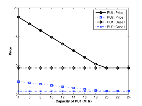
Figure 4: The change of prices when $q_{1}^{a}$ increases from 4MHz to 24MHz and $q_{2}^{a}$ is sufficiently large

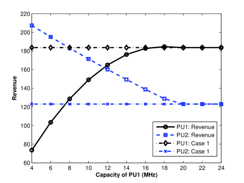
Figure 5: The change of revenues when $q_{1}^{a}$ increases from 4MHz to 24MHz and $q_{2}^{a}$ is sufficiently large

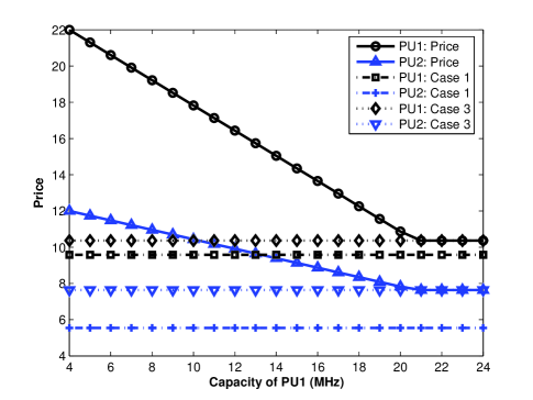
Figure 6: The change of prices when $q_{1}^{a}$ increases from 4MHz to 24MHz and $q_{2}^{a}$ is 15MHz

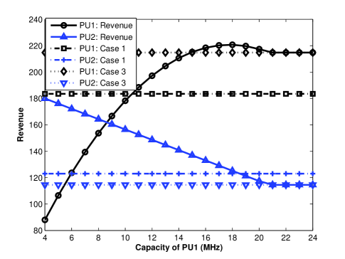
Figure 7: The change of revenues when $q_{1}^{a}$ increases from 4MHz to 24MHz and $q_{2}^{a}$ is 15MHz

We also illustrate the NEs of the leader-follower games. Let us first consider the case that both primary users have unlimited capacities. When PU1 is the leader and PU2 is the follower, the prices at the NE are $p_{1}^{*}=10.36$ and $p_{2}^{*}=5.69$. The corresponding spectrum demands are $q_{1}^{*}=17.81$ and $q_{2}^{*}=22.77$. When PU2 is the leader and PU1 is the follower, the prices and the spectrum demands at the NE are obtained: $p_{1}^{*}=9.75$, $p_{2}^{*}=6$, $q_{1}^{*}=19.50$ and $q_{2}^{*}=20.63$. Next, we study the NEs in the case that PU2 has sufficient spectrum and PU1’s capacity increases from 4MHz to 24MHz. The prices and revenues are compared in Fig.8 and 9 depending on which primary user is the leader. When the capacity of PU1 is less than 18MHz, the primary users have better prices and revenues if PU2 plays the role of market leader. One can easily draw a conclusion that the primary user with sufficient capacity, instead of the capacity-insufficient one, is profitable to be the leader in the duopoly Bertrand game. When we further increase the PU1’s capacity, the NEs become those in Case 1.

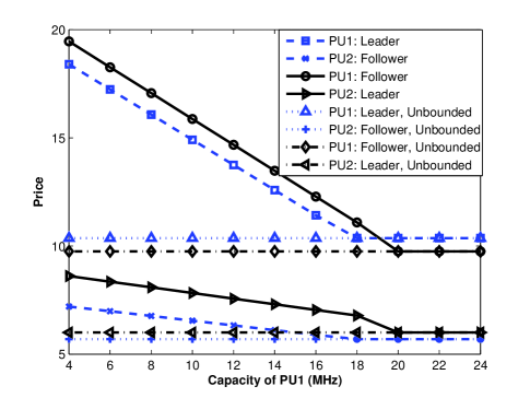
Figure 8: Prices verses PU1’s Capacity in the Leader-Follower Game for Sufficiently Large $q_{2}^{a}$

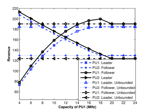
Figure 9: Revenues verses PU1’s Capacity in the Leader-Follower Game for Sufficiently Large $q_{2}^{a}$

5.2 Static Games with Type-II Constraints

In this subsection, we simulate the competitive pricing of the static spectrum game with type-II constraints. Specifically, we evaluate the price of per-unit spectrum and utilities by varying the capacity constraints and the QoS coefficient $\theta$. Note that the utility of primary users with type-II constraints contains $\theta\log(B_{i}/k_{i}^{(p)})$ for $i=1,2.$ Since they are constants, we only compare the parts in the utility functions that are related to the prices.

In the first set of experiments, the coefficient $\theta$ is set to 0.1, and the capacities of primary users increase from 4MHz to 24MHz. The prices of PU1 at the $NE$s are shown in Fig.10. The numerical experiments manifest that the prices of per-unit spectrum decreases with the increase of the primary users’ capacities. Fig.11 demonstrates the utilities of PU1, in which the utility is an increasing function with respect to the capacity of PU2. One can see that the utilities grow when PU1 and PU2 increase their capacities. In the second set of experiments, we aim to explore the relationship between $\theta$ and the price competition. Let $q_{1}^{a}$ and $q_{2}^{a}$ be 15MHz. When $\theta$ increases from 0.001 to 20, the prices of the primary users are shown in Fig.12. When $\theta$ becomes larger, the primary users are inclined to increase the prices to reduce the utility loss caused by the penalty functions.

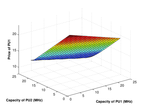
Figure 10: The price of PU1 in type-II model when both primary users increase spectrum capacities

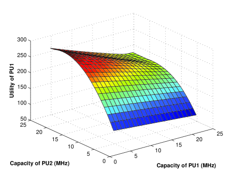
Figure 11: The revenue of PU1 in type-II model when both primary users increase spectrum capacities

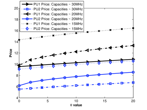
Figure 12: The price of PUs in type-II model when the parameter $\theta$ varies

5.3 Dynamic Game

We examine the dynamic behaviors of the noncooperative games with Type-I and Type-II constraints. Especially, the convergence rates of the proposed algorithms: StrictBEST, StrictBR and QoSBEST are evaluated. In the type-I model, we evaluate two settings that correspond to Case 1 and Case 2 respectively: $\{q_{1}^{a}=100MHz,q_{2}^{a}=100MHz\}$ and $\{q_{1}^{a}=10MHz,q_{2}^{a}=100MHz\}$. The QoS coefficient $\theta$ is set to 0.1 in the QoSBEST scheme. The price adaptations of StrictBEST and QoSBEST are shown in Fig.14-14. One can see that both StrictBEST and QoSBEST quickly converge to their individual equilibrium points. The dynamic adjustment of the StrictBR scheme is shown in Fig.16-16 where the learning rates $\gamma_{1,2}$ are both set to 0.01 and 0.03. The convergence rate of StrictBR depends on the learning rates $\gamma_{1}$ and $\gamma_{2}$. By cross-comparing Fig.16 and Fig.16, we observe that the convergence rate of Case 2 is faster than that of Case 1. This is because the adjustment strategy of PU1 does not have a conservative learning procedure in Case 2. In the StrictBR scheme, small learning rates can guarantee stability of the self-mapping system, however, at the cost of slow convergence speeds.

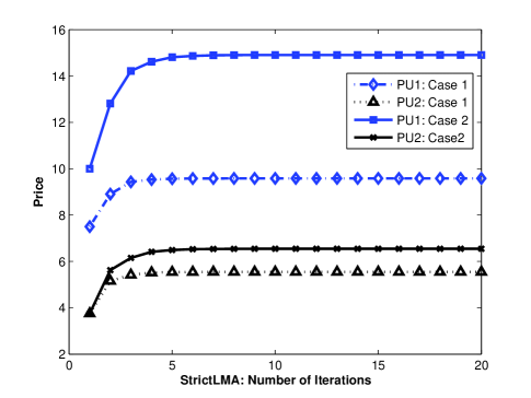
Figure 13: StrictBEST: Iteration of Prices

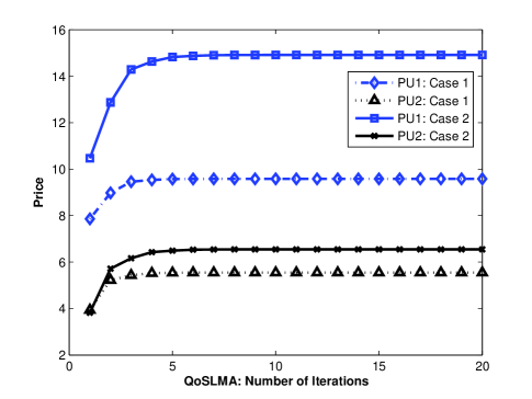
Figure 14: QoSBEST: Iteration of Prices

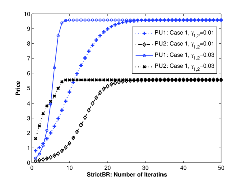
Figure 15: StrictBR: Iteration of Prices: $(q_{1}^{a}=100MHz,q_{2}^{a}=100MHz)$

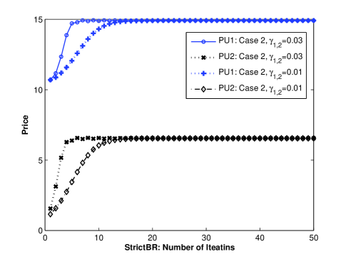
Figure 16: StrictBR: Iteration of Prices: $(q_{1}^{a}=10MHz,q_{2}^{a}=100MHz)$

5.4 Nonlinear Instability with Bounded Rationality

We explore the nonlinear dynamics such as bifurcation and chaos in the type-I duopoly game with bounded rationality. These complex behaviors are important because they reveal how prices of primary users evolve over time and how initial conditions influence the results of spectrum allocation. As is shown above, the StrictBR scheme can be applied in Case 1,2,3. Thus, we only consider Case 1 and Case 2 in the numerical studies since Case 3 is similar to Case 2.

Fig.18 shows the bifurcation diagram of Case 1 with respect to the learning rate $\gamma_{1}$. Here, the capacities of PU1 and PU2 are both 100MHz. The learning rate $\gamma_{2}$ is fixed to be 0.01 and the learning rate $\gamma_{1}$ increases from 0.01 to 0.09. The bifurcation diagram manifests that the attractor of Case 1 model is multivalued in term of parameter $\gamma_{1}$. One can also see in Fig.18 that there exists a stable NE when $\gamma_{1}$ is less than 0.0511. As $\gamma_{1}$ further increases, the NE become unstable and infinitely periodic doubling that leads to chaos eventually. The bifurcation diagram of Case 2 with respect to $\gamma_{2}$ is illustrated in Fig.18 where the capacity bounds are $q_{1}^{a}=$10MHz and $q_{2}^{a}=$100MHz. The learning rate $\gamma_{1}$ is 0.01 and the learning rate $\gamma_{2}$ grows from 0.01 to 0.06. When $\gamma_{2}$ is less than 0.0331, the StrictBR scheme converges to the unique NE of Case 2 duopoly model.

We show the graphs of strange attractors for Case 1 with the parameter constellation $(\gamma_{1},\gamma_{2})=(0.07,0.02)$ in Fig.20 and for Case 2 with the parameter constellation $(\gamma_{1},\gamma_{2})=(0.01,0.06)$ in Fig.20. Especially, Fig.20 exhibits a fractal structure similar to Henon attractor [14].

The Lyapunov exponent of a dynamical system characterizes the rate of separation of infinitesimally close trajectories. To analyze the parameter settings in which aperiodic behaviors occur, we compute the maximal Lyapunov exponents for the learning rates. If the maximal Lyapunov exponent is positive, the duopoly game with bounded rationality is chaotic. For Case 1, the maximal Lyapunov exponent is shown in Fig.22 as a function of the learning rate $\gamma_{1}$. When $\gamma_{1}$ is 0.0511, the maximal Lyapunov exponent becomes positive, which causes the first periodic doubling bifurcation in Fig.18. When $\gamma_{1}$ is greater than 0.0671, the maximal Lyapunov exponent is greater than 0. This indicates that the self-mapping price adaptation is a chaotic system. In Fig.22, we display the maximal Lyapunov exponent of Case 2 with respect to the learning rate $\gamma_{2}$. Here, the learning rate $\gamma_{1}$ is set to 0.01. When the learning rate $\gamma_{2}$ is around 0.0331, the duopoly game in Case 2 meets the first doubling bifurcation. With the increase of $\gamma_{2}$, the dynamic price adaptation becomes chaotic.

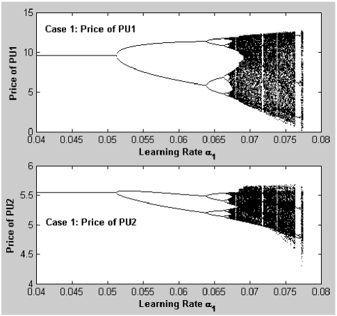
Figure 17: Bifurcation Diagram: $q_{1}^{a}=100MHz$ and $q_{2}^{a}=100MHz$

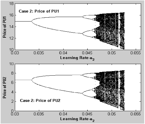
Figure 18: Bifurcation Diagram: $q_{1}^{a}=10MHz$ and $q_{2}^{a}=100MHz$

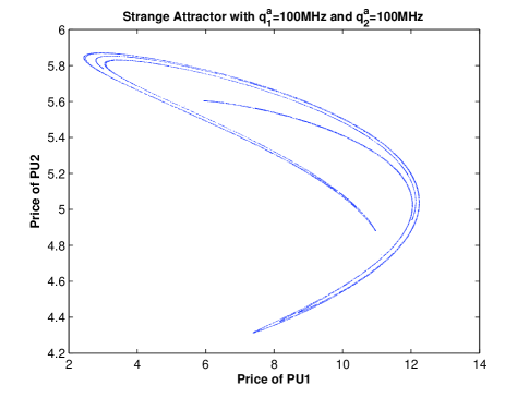
Figure 19: A Strange Attractor for the Following Parameters: Initial $p_{1}=5$, Initial $p_{2}=5$, $\gamma_{1}=0.07$, $\gamma_{2}=0.02$, $q_{1}^{a}=100MHz$ and $q_{2}^{a}=100MHz$

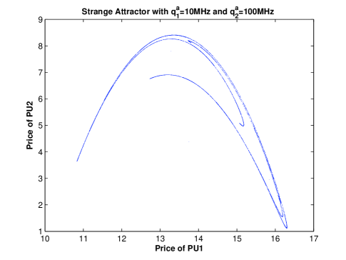
Figure 20: A Strange Attractor for the Following Parameters: Initial $p_{1}=5$, Initial $p_{2}=5$, $\gamma_{1}=0.01$, $\gamma_{2}=0.06$, $q_{1}^{a}=10MHz$ and $q_{2}^{a}=100MHz$

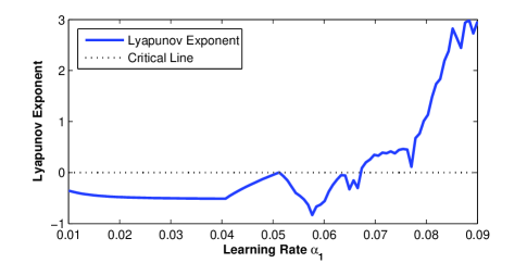
Figure 21: Lyapunov Exponent: $q_{1}^{a}=100MHz$ and $q_{2}^{a}=100MHz$

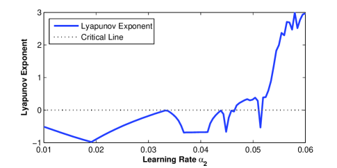
Figure 22: Lyapunov Exponent: $q_{1}^{a}=10MHz$ and $q_{2}^{a}=100MHz$

6 Related Work

The rapid development of wireless communication systems in the past two decades have resulted in the great needs of a finite and scarce resource: wireless spectrum. On the other hand, existing wireless devices operate in the fixed frequency bands, which can be very inefficient in terms of spectrum utilization. The research carried out by FCC shows that temporal and geographical variations in the utilization of the assigned spectrum range from 15% to 85% [4]. As a promising technology, dynamic spectrum access is brought forward in the design of next generation wireless communication systems. The under-utilized spectrum bands can be detected and exploited by the users equipped with cognitive radios. For the detailed information, interested readers can refer to recent surveys in [5] and [6].

One key feature of dynamic spectrum access is how the primary users (or wireless service provides) and the secondary users (or end users) share the spectrum efficiently and fairly. In particular, the dynamic spectrum sharing may involve selling and purchasing processes. Thus, it is natural to study the interactions of network components for dynamic spectrum sharing from the perspective of economics. The existing work can be mainly grouped into two classes: auction-based [7, 8, 9] and price-based [2, 10, 3]. Authors in the seminal work [7] target at the dishonest bidding issues in an eBay-like dynamic spectrum market. A truthful and computationally efficient auction mechanism is presented to perform dynamic spectrum allocation. To maximize revenue and spectrum utilization, authors in [20] propose a real-time spectrum auction framework to distribute spectrum among a large number wireless users under interference constraints. Zhu and Liu [8] propose an auction-based collusion-resistant dynamic spectrum allocation approach to combat user collusion in cognitive wireless networks. An economic framework is also presented in [9] to model the spectrum allocation to wireless service providers (WSPs) and the interaction of of end users with the WSPs, but the competition among WSPs is not the focus. Leveraging on microeconomics inspired mechanisms, authors in [19] develop both bargaining and auction based mechanisms to find the most optimized allocation pattern for a given area and allocation duration. Some other auction based spectrum sharing mechanisms can be found in [22, 23, 23, 25, 26]. In the price-based class, Niyato and Hossain [2] introduce the oligopoly pricing theory to characterize the interactions between the primary users and the secondary users. In the oligopoly spectrum market, a commonly used quadratic utility is adopted to quantify the spectrum demand of the secondary service, and each primary user aims to maximize the individual profit. In another work [10], they consider the dynamic spectrum sharing among a primary user and multiple secondary users. They formulate the problem as an oligopoly market competition and use a noncooperative game to obtain the Nash Equilibrium. Very recently in an important work [3], Jia and Zhang formulate the price and the spectrum competitions as a two-stage non-cooperative game that is inspired by the theoretic analyses of Cournot and Bertrand games [16, 17]. In [21], authors consider a primary user employing CDMA at the physical layer who aims to lease its spectrum within a certain geographic subregion. [28] studies a revenue maximization problem in a Stackelberg game, where spectrum owner, primary users and secondary users are the players for opportunistic spectrum access. Besides, authors in [27] build a game theoretic model to investigate whether light regulation in the form of etiquette protocols, device design and bargaining amongst users can avoid the tragedy of common in unlicensed spectrum. In terms of nonlinear dynamics in the economics, authors in [15] have shown that the bounded rationality can cause chaotic behaviors in a Cournot duopoly.

7 Conclusion

This paper suggests an economic framework for dynamic spectrum allocation in the emerging cognitive radio networks. The primary users serve as the spectrum brokers that lease the excessive frequency to the secondary users for monetary payoff. We present oligopoly Bertrand market models to characterize the capacity-limited spectrum sharing with two types of constraints: the strict constraints (type-I) and the QoS penalty functions (type-II). In the type-I oligopoly market, we present a low-complexity scheme to search the NE and prove its uniqueness. Especially, when the number of primary users reduces to two, we demonstrate the interesting revenue gaps in the leader-follower game. Two iterative algorithm, StrictBEST and StrictBR, are presented to adjust the prices when the primary users only possesses the local market information. In the type-II model, we prove the existence of unique NE and propose a price updating algorithm named QoSBEST. Numerical examples validate our analysis and manifest the effectiveness of our proposals. In particular, we experimentally show the representative nonlinear dynamics in the StrictBR algorithm such as bifurcations, chaotic maps as well as Lyapunov exponents. Our future research will be placed on the competitive pricing in more complicated markets, e.g. the number of active primary users are not deterministic.

APPENDIX

Lemma 1: The matrix $\mathbf{T}$ is positive definite if the market parameters has $\beta_{i}>\mu>0$ for all $i\in\mathcal{N}$.

Proof: Given a $N\times 1$ nonzero, real vector $\mathbf{x}$, there has,

$$\mathbf{x}^{T}\mathbf{T}\mathbf{x}=\mathbf{x}^{T}\left[\begin{array}[]{cccc}\beta_{1}&\mu&\ldots&\mu\\ \mu&\beta_{2}&\ldots&\mu\\ \vdots&\vdots&\ddots&\vdots\\ \mu&\mu&\ldots&\beta_{N}\end{array}\right]\mathbf{x}$$ (145)

$$=\mathbf{x}^{T}\big{(}\mu\left[\begin{array}[]{cccc}1&1&\ldots&1\\ 1&1&\ldots&1\\ \vdots&\vdots&\ddots&\vdots\\ 1&1&\ldots&1\end{array}\right]+\left[\begin{array}[]{cccc}\beta_{1}-\mu&0&\ldots&0\\ 0&\beta_{2}-\mu&\ldots&0\\ \vdots&\vdots&\ddots&\vdots\\ 0&0&\ldots&\beta_{N}-\mu\end{array}\right]\big{)}\mathbf{x}$$ (154)

$$=\mu(\sum_{i=1}^{N}x_{i})^{2}+\sum_{i=1}^{N}(\beta_{i}-\mu)x_{i}^{2}>0.$$ (155)

Hence, the matrix $\mathbf{T}$ is positive definite if $\beta_{i}>\mu>0$ for all $i\in\mathcal{N}$.  

Lemma 2: The parameters that characterize demand-price function in Eqn.(17), i.e.$\;b_{i}$ and $c_{ij}$ $(i\neq j)$, are positive, given the conditions $\beta_{i}>\mu>0$ for all $i,j\in\mathcal{N}$.

Proof:We use Cramer’s rule to compute the invertible matrix of $\mathbf{T}$ as follows,

$$\mathbf{T}^{-1}={1\over\begin{vmatrix}\mathbf{T}\end{vmatrix}}\left(\mathbf{U}_{ij}\right)^{T}={1\over\begin{vmatrix}\mathbf{T}\end{vmatrix}}\left(\mathbf{U}_{ji}\right)={1\over\begin{vmatrix}\mathbf{T}\end{vmatrix}}\begin{pmatrix}\mathbf{U}_{11}&\mathbf{U}_{21}&\cdots&\mathbf{U}_{n1}\\ \mathbf{U}_{12}&\mathbf{U}_{22}&\cdots&\mathbf{U}_{n2}\\ \vdots&\vdots&\ddots&\vdots\\ \mathbf{U}_{1n}&\mathbf{U}_{2n}&\cdots&\mathbf{U}_{nn}\\ \end{pmatrix},$$ (156)

where $|\mathbf{T}|$ is the determinant of $\mathbf{T}$ and $\mathbf{U}_{ij}$ is the matrix cofactor. Then, the variable $b_{i}$ can be expressed as $b_{i}=\frac{\mathbf{U}_{ii}}{|T|}$. The variables $c_{ij}$ can be written as $c_{ij}=\frac{\mathbf{U}_{ji}}{{|T|}}$ when $i\neq j$. Since $\mathbf{T}$ is positive definite, $|\mathbf{T}|$ is greater than 0. The cofactor $\mathbf{U}_{ii}$ is

$$\mathbf{U}_{ii}={1\over\begin{vmatrix}\mathbf{T}\end{vmatrix}}\left|\begin{array}[]{cccccc}\beta_{1}&\ldots&\ldots&\ldots&\ldots&\mu\\ \vdots&\ddots&\ldots&\ldots&\ldots&\mu\\ \vdots&\ldots&\beta_{i-1}&\ldots&\ldots&\mu\\ \vdots&\ldots&\ldots&\beta_{i+1}&\ldots&\mu\\ \vdots&\ldots&\ldots&\ldots&\ddots&\mu\\ \mu&\ldots&\ldots&\ldots&\ldots&\beta_{N}\end{array}\right|,$$ (163)

where all the elements except diagonal ones in the above determinant are $\mu$. According to Lemma 1, one can easily find $b_{i}>0\;$ for all $i\in\mathcal{N}$. Similarly, we can also prove that $\mathbf{U}_{ji}$ is negative for all $i,j\in\mathcal{N}$ and $i\neq j$. Thus, the market parameters $c_{ij}$ are all positive for $i,j\in\mathcal{N}$ and $i\neq j$. The only difference lies in that we need to exchange certain columns in the determinant before applying Lemma 1.  

Lemma 3: The matrix $\mathbf{Q}(M_{k})$ is positive definite if $\beta_{i}>\mu>0$ for all $i\in\mathcal{N}$ in the utility function.

Proof: We prove this lemma by contradiction.

$$\mathbf{Q}(M_{k}) = \left[\begin{array}[]{ccccc}b_{1}&-c_{12}&\ldots&\ldots&-c_{1N}\\ -c_{21}&b_{2}&\ldots&\ldots&-c_{2N}\\ \vdots&\vdots&\ldots&\ldots&\vdots\\ \vdots&\vdots&\ldots&\ldots&\vdots\\ -c_{N1}&-c_{N2}&\ldots&\ldots&b_{N}\end{array}\right]+\left[\begin{array}[]{ccccc}0&\ldots&\ldots&\ldots&\ldots\\ \vdots&\ldots&\ldots&\ldots&\ldots\\ 0&\ldots&b_{M_{k}+1}&\ldots&0\\ \vdots&\ldots&\ldots&\ldots&\vdots\\ 0&\ldots&\ldots&\ldots&b_{N}\end{array}\right]$$ (174)

$$= \left[\begin{array}[]{cccc}\beta_{1}&\mu&\ldots&\mu\\ \mu&\beta_{2}&\ldots&\mu\\ \vdots&\vdots&\ddots&\vdots\\ \mu&\mu&\ldots&\beta_{N}\end{array}\right]^{-1}+\left[\begin{array}[]{ccccc}0&\ldots&\ldots&\ldots&\ldots\\ \vdots&\ldots&\ldots&\ldots&\ldots\\ 0&\ldots&b_{M_{k}+1}&\ldots&0\\ \vdots&\ldots&\ldots&\ldots&\vdots\\ 0&\ldots&\ldots&\ldots&b_{N}\end{array}\right].$$ (184)

We assume that the matrix $Q(M_{k})$ is singular. Thus, there exists a non-zero vector $\mathbf{x}$ that has $\mathbf{x}^{T}Q(M_{k})\mathbf{x}=0$. Because the matrix $\mathbf{T}$ is positive definite, it inverse matrix is also positive definite. We then rewrite $\mathbf{x}^{T}Q(M_{k})\mathbf{x}$ as:

$$\mathbf{x}^{T}Q(M_{k})\mathbf{x}=\mathbf{x}^{T}\mathbf{T}^{-1}\mathbf{x}+\sum_{i=M_{k}+1}^{N}b_{i}x_{i}^{2}\geq\mathbf{x}^{T}\mathbf{T}^{-1}\mathbf{x}>0.$$

for any non-zero vector $\mathbf{x}$.  

Lemma 4: The set of capacity-insufficient primary users in the $k-1^{th}$ step is a subset of that in the $k^{th}$ step.

Proof: Denote $M_{k}$ and $\{M_{k}\}$ to be the number and the set of capacity-insufficient primary users in the $k^{th}$ search respectively. Denote $p_{i}^{(k)}$ to be the price of primary user $i$ in the $k^{th}$ search. At the beginning, $M_{0}$ is equal to 0.

In the first search, there must have $M_{1}>0$. Otherwise, all the primary users have sufficient capacities. Without loss of generality, we look at the the $k^{th}$ search result.

The $k^{th}$ search is based on a priori knowledge that the primary users in the set $\{M_{k-1}\}$ are capacity-insufficient. We assume that the $k^{th}$ search finds out $M_{k}$ capacity-insufficient primary users. Hence, the newly found primary users satisfy

$$\frac{a_{i}+\sum_{j\neq i}c_{ij}p_{j}^{(k)}}{2}>q_{i}^{a},\;\;\;\;\;\forall i=M_{k-1}+1,\cdots,M_{k}.$$ (185)

Because the price strategy of the $i^{th}$ new capacity-insufficient PU is $\frac{a_{i}+\sum_{j\neq i}c_{ij}p_{j}^{(k)}}{2b_{i}}$, the above equality is equivalent to $b_{i}p_{i}^{(k)}>q_{i}^{a}$.

Next, we compare the price vector of the $k^{th}$ and the $k-1^{th}$ searches. According to Eqn.(54), an alternative form of price difference is expressed as

$$\mathbf{Q}(M_{k})\mathbf{p}^{(k)}-\mathbf{Q}(M_{k-1})\mathbf{p}^{(k-1)}$$

$$=\mathbf{Q}(M_{k-1})\cdot(\mathbf{p}^{(k)}-\mathbf{p}^{(k-1)})-\left[\begin{array}[]{c}\mathbf{0}\\ b_{M_{k-1}+1}p_{M_{k-1}+1}^{(k)}\\ \vdots\\ b_{M_{k}}p_{M_{k}}^{(k)}\\ \mathbf{0}\end{array}\right]=-\left[\begin{array}[]{c}\mathbf{0}\\ q_{M_{k-1}+1}^{a}\\ \vdots\\ q_{M_{k}}^{a}\\ \mathbf{0}\end{array}\right]$$ (196)

Submit the conditions $b_{i}^{k}q_{i}^{(k)}>q_{i}^{a}$ for all $i=M_{k-1}+1,\cdots,M_{k}$ to the above equation, we obtain

$$\mathbf{Q}(M_{k-1})\cdot(\mathbf{p}^{(k)}-\mathbf{p}^{(k-1)})>0.$$ (197)

Because $\mathbf{Q}(M_{k-1})$ is a Stieltjes matrix, it is inverse nonnegative. Therefore, all elements in the vector $\mathbf{p}^{(k)}-\mathbf{p}^{(k-1)}$ are nonnegative. This means that the prices of all primary users do not decrease in each search. For the primary users in the set $M_{k-1}$, their optimal spectrum demands are $\frac{a_{i}+\sum_{j\neq i}c_{ij}p_{j}^{(k)}}{2}$, which is also nondecreasing. To sum up, when a primary user is found to be capacity-insufficient in the $k-1^{th}$ round, it still lacks of capacity in the next search.  

Theorem 2: Consider a type-I oligopoly spectrum market in Eqn.(17), there exists a unique Nash Equilibrium.

Proof: We prove this theorem via two steps by contradiction. First, we will show that there exists a unique NE if the capacity-insufficient PUs are unchangeable. In the second step, we prove that the set of PUs that have insufficient capacities is unique in the oligopoly market.

As is mentioned earlier, a selfish PU decides the prices according to the rule Eqn.(44) if the capacity is less than the best demand, and the rule Eqn.(45) otherwise. Provided a market with $N$ PUs, we can find that $M$ of them are capacity-insufficient through the proposed search method. The price vector at the NE, $\mathbf{p}^{*}$, can be computed by

$$\mathbf{p}^{*}=[\mathbf{Q}(M)]^{-1}\cdot\mathbf{a}(M),$$

where $\mathbf{Q}$ is a positive-definite matrix. Hence, when the set of capacity-insufficient PUs are determined, there is a unique Nash Equilibrium.

Next, we demonstrate that there has a unique set of capacity-insufficient primary users. The primary users in the set $\mathcal{N}$ are grouped into four mutually exclusive classes: $\mathcal{N}_{1}$, $\mathcal{N}_{2}$, $\mathcal{N}_{3}$ and $\mathcal{N}_{4}$. PUs in the sets $\mathcal{N}_{1}$ and $\mathcal{N}_{2}$ are capacity-insufficient in the iterative search (i.e. $\mathcal{M}=\mathcal{N}_{1}\cup\mathcal{N}_{2}$), but the PUs in the sets $\mathcal{N}_{3}$ and $\mathcal{N}_{4}$ have enough capacities. The price vector at the NE is denoted as $\mathbf{p}^{*}=\{p_{1}^{*},p_{2}^{*},\cdots,p_{N}^{*}\}$. At the NE, the PUs must have

$$\frac{a_{i}+\sum_{j\neq i}c_{i,j}p_{j}^{*}}{2}>q_{i}^{a}\;\;\Rightarrow\;\;b_{i}p_{i}^{*}>q_{i}^{a}\;\;\;\forall i\in\mathcal{N}_{1};$$ (198)

$$\frac{a_{i}+\sum_{j\neq i}c_{i,j}p_{j}^{*}}{2}>q_{i}^{a}\;\;\Rightarrow\;\;b_{i}p_{i}^{*}>q_{i}^{a}\;\;\;\forall i\in\mathcal{N}_{2};$$ (199)

$$\frac{a_{i}+\sum_{j\neq i}c_{i,j}p_{j}^{*}}{2}\leq q_{i}^{a}\;\;\Rightarrow\;\;b_{i}p_{i}^{*}\leq q_{i}^{a}\;\;\;\forall i\in\mathcal{N}_{3};$$ (200)

$$\frac{a_{i}+\sum_{j\neq i}c_{i,j}p_{j}^{*}}{2}\leq q_{i}^{a}\;\;\Rightarrow\;\;b_{i}p_{i}^{*}\leq q_{i}^{a}\;\;\;\forall i\in\mathcal{N}_{4}.$$ (201)

Assume that there exists a different set of PUs that are also capacity-insufficient. For general purpose, we express this new set as $\mathcal{N}_{1}\cup\mathcal{N}_{3}$ and the capacity-sufficient set as $\mathcal{N}_{2}\cup\mathcal{N}_{4}$. Note that the above PU sets can be empty, but has a union of $\mathcal{N}$. Since there has a different set of capacity-insufficient PUs, we can find another NE price vector $\mathbf{p}^{{\dagger}}$ that also have

$$\frac{a_{i}+\sum_{j\neq i}c_{i,j}p_{j}^{{\dagger}}}{2}>q_{i}^{a}\;\;\Rightarrow\;\;b_{i}p_{i}^{{\dagger}}>q_{i}^{a}\;\;\;\forall i\in\mathcal{N}_{1};$$ (202)

$$\frac{a_{i}+\sum_{j\neq i}c_{i,j}p_{j}^{{\dagger}}}{2}>q_{i}^{a}\;\;\Rightarrow\;\;b_{i}p_{i}^{{\dagger}}>q_{i}^{a}\;\;\;\forall i\in\mathcal{N}_{3};$$ (203)

$$\frac{a_{i}+\sum_{j\neq i}c_{i,j}p_{j}^{{\dagger}}}{2}\leq q_{i}^{a}\;\;\Rightarrow\;\;b_{i}p_{i}^{{\dagger}}\leq q_{i}^{a}\;\;\;\forall i\in\mathcal{N}_{2};$$ (204)

$$\frac{a_{i}+\sum_{j\neq i}c_{i,j}p_{j}^{{\dagger}}}{2}\leq q_{i}^{a}\;\;\Rightarrow\;\;b_{i}p_{i}^{{\dagger}}\leq q_{i}^{a}\;\;\;\forall i\in\mathcal{N}_{4}.$$ (205)

Here, one can easily find there have $p_{i}^{{\dagger}}>p_{i}^{*}$ for $i\in\mathcal{N}_{3}$ and $p_{i}^{*}>p_{i}^{{\dagger}}$ for $i\in\mathcal{N}_{2}$. According to the market model, the prices at the NEs can be expressed in terms of spectrum demands $q_{i}^{*}$ and $q_{i}^{{\dagger}}$. Then, $p_{i}^{{\dagger}}$ and $p_{i}^{*}$ in the sets $\mathcal{N}_{2}$ and $\mathcal{N}_{4}$ are written by,

$$\!\!\!\!\!\!\!\!\!\!p_{i}^{*}\!=\!\alpha_{i}-(\beta_{i}-\mu)q_{i}^{a}-\mu\sum_{j\in\mathcal{N}_{1}}q_{j}^{a}-\mu\sum_{j\in\mathcal{N}_{2}}q_{j}^{a}-\mu\sum_{j\in\mathcal{N}_{3}}q_{j}^{*}-\mu\sum_{j\in\mathcal{N}_{4}}q_{j}^{*},\;\forall i\in\mathcal{N}_{2};$$ (206)

$$\!\!\!\!\!\!\!\!\!\!p_{i}^{*}\!=\!\alpha_{i}-(\beta_{i}-\mu)q_{i}^{*}-\mu\sum_{j\in\mathcal{N}_{1}}q_{j}^{a}-\mu\sum_{j\in\mathcal{N}_{2}}q_{j}^{a}-\mu\sum_{j\in\mathcal{N}_{3}}q_{j}^{*}-\mu\sum_{j\in\mathcal{N}_{4}}q_{j}^{*},\;\forall i\in\mathcal{N}_{3};$$ (207)

$$\!\!\!\!\!\!\!\!\!\!p_{i}^{{\dagger}}\!=\!\alpha_{i}-(\beta_{i}-\mu)q_{i}^{{\dagger}}-\mu\sum_{j\in\mathcal{N}_{1}}q_{j}^{a}-\mu\sum_{j\in\mathcal{N}_{2}}q_{j}^{{\dagger}}-\mu\sum_{j\in\mathcal{N}_{3}}q_{j}^{a}-\mu\sum_{j\in\mathcal{N}_{4}}q_{j}^{{\dagger}},\;\forall i\in\mathcal{N}_{2};$$ (208)

$$\!\!\!\!\!\!\!\!\!\!p_{i}^{{\dagger}}\!=\!\alpha_{i}-(\beta_{i}-\mu)q_{i}^{a}-\mu\sum_{j\in\mathcal{N}_{1}}q_{j}^{a}-\mu\sum_{j\in\mathcal{N}_{2}}q_{j}^{{\dagger}}-\mu\sum_{j\in\mathcal{N}_{3}}q_{j}^{a}-\mu\sum_{j\in\mathcal{N}_{4}}q_{j}^{{\dagger}},\;\forall i\in\mathcal{N}_{3}.$$ (209)

Recall that the conditions in Eqn.(199),(200),(203) and (204) present the results: $p_{i}^{{\dagger}}>p_{i}^{*}$ for $i\in\mathcal{N}_{3}$ and $p_{i}^{*}>p_{i}^{{\dagger}}$ for $i\in\mathcal{N}_{2}$. Hence, we have the following inequality

$$p_{i}^{*}+p_{l}^{{\dagger}}>p_{i}^{{\dagger}}+p_{l}^{*}\;\;\;\forall i\in\mathcal{N}_{2},l\in\mathcal{N}_{3}.$$ (210)

Submit Eqn.(206)-(209) to Eqn.(210) and cancel out the common items, we obtain the inequality

$$(\beta_{i}-\mu)q_{i}^{{\dagger}}+(\beta_{l}-\mu)q_{i}^{*}>(\beta_{i}-\mu)q_{i}^{a}+(\beta_{l}-\mu)q_{l}^{a}\;\;\;\forall i\in\mathcal{N}_{2},l\in\mathcal{N}_{3}.$$ (211)

Obviously, the above inequality is not true provided the market conditions $\beta_{i}>\mu$ for $i\in\mathcal{N}$. Thus, there is a unique set of capacity-insufficient primary users, resulting in a unique Nash Equilibrium in the oligopoly spectrum game.  

Theorem 4: The QoSBEST algorithm converges to the unique NE if the market parameters are positive as well as $b_{1}>c>0$ and $b_{2}>c>0$.

Proof: Assume the NE prices of PU1 and PU2 are $p_{1}^{*}$ and $p_{2}^{*}$. We start from time $t$ and solve the equation in Eqn.(137). Although $p_{1}(t+1)$ in Eqn.(137) has two roots, one can easily check their feasibility by submitting these roots to the equation $q_{1}(t)=a_{1}-b_{1}p_{1}(t+1)+cp_{2}(t)$. After excluding the infeasible root, the unique price of PU1 is expressed as

$$p_{1}(t+1)=\frac{(3a_{1}+3cp_{2}(t)-2q_{1}^{a})+\sqrt{(a_{1}+cp_{2}(t)-2q_{1}^{a})^{2}+8b_{1}\theta}}{4b_{1}},$$

and the optimal price of PU1 is written as

$$p_{1}^{*}=\frac{(3a_{1}+3cp_{2}^{*}-2q_{1}^{a})+\sqrt{(a_{1}+cp_{2}^{*}-2q_{1}^{a})^{2}+8b_{1}\theta}}{4b_{1}},$$

In order to compare $p_{1}(t+1)$ and $p_{1}^{*}$, we consider four cases with regard to different $p_{2}(t)$ and $p_{2}^{*}$.

Case 1: $a_{1}+cp_{2}(t)-2q_{1}^{a}\geq 0$ and $a_{1}+cp_{2}^{*}-2q_{1}^{a}\geq 0$;

The difference between $p_{1}(t+1)$ and $p_{1}^{*}$ is,

$$p_{1}(t+1)-p_{1}^{*}=\frac{3c(p_{2}(t)-p_{2}^{*})}{4b_{1}}+\frac{\sqrt{(a_{1}+cp_{2}(t)-2q_{1}^{a})^{2}+8b_{1}\theta}-\sqrt{(a_{1}+cp_{2}^{*}-2q_{1}^{a})^{2}+8b_{1}\theta}}{4b_{1}}.$$

If $p_{2}(t)\geq p_{2}^{*}$, there has $a_{1}+cp_{2}(t)-2q_{1}^{a}>a_{1}+cp_{2}^{*}-2q_{1}^{a}>0$. According to Lemma 5, the following inequality holds,

$$p_{1}(t+1)-p_{1}^{*}\leq\frac{c(p_{2}(t)-p_{2}^{*})}{b_{1}}.$$ (212)

On the other hand, if $p_{2}(t)<p_{2}^{*}$, there has $0<a_{1}+cp_{2}(t)-2q_{1}^{a}<a_{1}+cp_{2}^{*}-2q_{1}^{a}$. Based on Lemma 5, we can obtain the following inequality,

$$p_{1}(t+1)-p_{1}^{*}>\frac{c(p_{2}(t)-p_{2}^{*})}{b_{1}}.$$ (213)

Combine Eqn.(212) and (213) together, we have,

$$|p_{1}(t+1)-p_{1}^{*}|\leq\frac{c}{b_{1}}|p_{2}(t)-p_{2}^{*}|.$$ (214)

Case 2: $a_{1}+cp_{2}(t)-2q_{1}^{a}<0$ and $a_{1}+cp_{2}^{*}-2q_{1}^{a}<0$;

If $p_{2}(t)\leq p_{2}^{*}$, there has $0<2q_{1}^{a}-(a_{1}+cp_{2}^{*})\leq 2q_{1}^{a}-(a_{1}+cp_{2}(t))$. Similarly, we calculate the difference between $p_{1}(t+1)$ and $p_{1}^{*}$,

$$\frac{3c(p_{2}(t)-p_{2}^{*})}{4b_{1}}\leq p_{1}(t+1)-p_{1}^{*}\leq\frac{c(p_{2}(t)-p_{2}^{*})}{2b_{1}}.$$ (215)

Otherwise, if $p_{2}(t)>p_{2}^{*}$, the difference between $p_{1}(t+1)$ and $p_{1}^{*}$ satisfies,

$$\frac{c(p_{2}(t)-p_{2}^{*})}{2b_{1}}\leq p_{1}(t+1)-p_{1}^{*}\leq\frac{3c(p_{2}(t)-p_{2}^{*})}{4b_{1}}.$$ (216)

The above analysis manifests that the following inequalities hold,

$$\frac{c}{2b_{1}}|p_{2}(t)-p_{2}^{*}|\leq|p_{1}(t+1)-p_{1}^{*}|\leq\frac{3c}{4b_{1}}|p_{2}(t)-p_{2}^{*}|.$$ (217)

Case 3: $a_{1}+cp_{2}(t)-2q_{1}^{a}\geq 0$ and $a_{1}+cp_{2}^{*}-2q_{1}^{a}<0$;

The case 3 also implies $p_{2}(t)\geq p_{2}^{*}$. According to Lemma 5, the following inequalities hold,

$$-c(p_{2}(t)-p_{2}^{*})\leq\sqrt{(a_{1}+cp_{2}(t)-2q_{1}^{a})^{2}+8b_{1}\theta}-\sqrt{(2q_{1}^{a}-(a_{1}+cp_{2}^{*}))^{2}+8b_{1}\theta}\leq c(p_{2}(t)-p_{2}^{*}).$$

Therefore, the difference between $p_{1}(t+1)$ and $p_{1}^{*}$ satisfies,

$$\frac{c}{2b_{1}}|p_{2}(t)-p_{2}^{*}|\leq|p_{1}(t+1)-p_{1}^{*}|\leq\frac{c}{b_{1}}|p_{2}(t)-p_{2}^{*}|.$$ (218)

Case 4: $a_{1}+cp_{2}(t)-2q_{1}^{a}<0$ and $a_{1}+cp_{2}^{*}-2q_{1}^{a}\geq 0$;

This case implies $p_{2}(t)\leq p_{2}^{*}$. Using the similar method as that in Case 3, we obtain the same inequality in (218). Combine all the analytic results together, we can see the distance between $p_{1}(t+1)$ and $p_{1}^{*}$ has $|p_{1}(t+1)-p_{1}^{*}|\leq\frac{c}{b_{1}}|p_{2}(t)-p_{2}^{*}|$. Using the similar steps, we can easily find that in slot $(t+1)$, the following inequality holds,

$$|p_{2}(t+2)-p_{2}^{*}|\leq\frac{c}{b_{2}}|p_{1}(t+1)-p_{1}^{*}|\leq\frac{c^{2}}{b_{1}b_{2}}|p_{2}(t)-p_{2}^{*}|\leq(\frac{c^{2}}{b_{1}b_{2}})^{\frac{t}{2}}|p_{2}(0)-p_{2}^{*}|,$$ (219)

where $p_{2}(0)$ is the initial price of PU2. Given the conditions $b_{1}>c$ and $b_{2}>c$, the QoSBEST algorithm converges to the unique NE.

References

• [1] X. Vives, “Oligopoly Pricing”, The MIT Press. Cambridge, MA., 1999.
• [2] D. Niyato, E. Hossain, “Competitive Pricing for Spectrum Sharing in Cognitive Radio Networks: Dynamic Game, Inefficiency of Nash Equilibrium, and Collusion”, IEEE Journal on Selected Areas in Communication. Vol.26, No.1, pp:192-202, 2008.
• [3] J.C. Jia, Q. Zhang, “Competitions and Dynamics of Duopoly Wireless Service Providers in Dynamic Spectrum Market”, Proc. of ACM Mobihoc’08. pp:313-322, Hong Kong, 2008.
• [4] FCC, ET Docket No. 03-222. “Notice of proposed rule making and order”, December 2003.
• [5] I.F. Akyildiz, W.Y. Lee, M.C. Vuran and S. Mohanty, “NeXt generation/dynamic spectrum access/cognitive radio wireless networks: A survey”, Elsevier Computer Networks. Vol.50, pp:2127-2159, 2006.
• [6] S. Haykin, “Cognitive radio: brain-empowered wireless communications”, IEEE Journal on Selected Areas in Communications, Vol.23, No.2, pp:201 C220, 2005.
• [7] X. Zhou, S. Gandhi, S. Suri and H.T. Zheng, “eBay in the Sky: Strategy-Proof Wireless Spectrum Auctions”, Proc. of ACM Mobicom’08, San Francisco, 2008.
• [8] Zhu Ji and K.J.R. Liu, “Multi-Stage Pricing Game for Collusion-Resistant Dynamic Spectrum Allocation”, IEEE Journal on Selected Areas in Communications, VOL.26, NO.1, pp:182-191, 2008.
• [9] S. Sengupta, M. Chatterjee and S. Ganguly, “An Economic Framework for Spectrum Allocation and Service Pricing with Competitive Wireless Service Providers”, Proc. of IEEE Dyspan’07, pp:89-98, 2007.
• [10] D. Niyato and E. Hossain, “Competitive Spectrum Sharing in Cognitive Radio Networks: A Dynamic Game Approach”, IEEE Trans. Wireless Communication, Vol.7, No.7, pp:2651-2660, 2008.
• [11] G.I. Bischi, M. Galletgatti, A. Naimzada, “Symmetry-breaking bifurcations and representative firm in dynamic duopoly games”, Annals of Operations Research Vol.89, pp:253-272, 1999.
• [12] G.I. Bischi, A. Naimzada, “Global analysis of a dynamic duopoly game with bounded rationality”. In: J.A. Filar, et.al, Advances in Dynamic Games and Applications, Vol.5, Birkhauser, 2000.
• [13] G.I. Bischi, F. Lamantia, “Coexisting attractors and complex basins in discrete-time economics models”. In: M. Lines (Ed.), Nonlinear Dynamical Systems in Economics, Springer, pp:187-231, 2005.
• [14] M. Henon, “A Two Dimensional Mapping with a Strange Attractor”, Comm. Math. Phys.. pp:69-77, 1976.
• [15] H.N. Agiza, A.A. Elsadany, “Nonlinear Dynamics in the Cournot Duopoly Game with Heterogeneous Players”, Physica A, Vol.320, pp:512-524, 2003.
• [16] A. Shaked and J. Sutton, “Relaxing Price Competition Through Product Differentiation”, Review of Economic Studies, Vol.49, No.1, pp:3-13, 1982.
• [17] N. Singh and X. Vives, “Price and Quantity Competition in a Differentiated Duopoly”, RAND Journal of Economics, Vol.15, No.4, pp:546-554, 1984.
• [18] D.M. Young, “Iterative Solution of Large Linear Systems”, Academic Publisher, 2003.
• [19] D. Grandblaise, C. Kloeck, T. Renk, et.al, “Microeconomics Inspired Mechanisms to Manage Dynamic Spectrum Allocation”, Proc. of IEEE Dyspan’07, pp:452-461, 2007.
• [20] S. Gandhi, C. Buragohain, L.L. Gao, H.T. Zheng, and S. Suri, “A General Framework for Wireless Spectrum Auctions”, Proc. of IEEE Dyspan’07, pp:22-33, 2007.
• [21] A.A. Daoud, M. Alanyali, and D. Starobinski “Secondary Pricing of Spectrum in Cellular CDMA Networks”, Proc. of IEEE Dyspan’07, pp:535-542, 2007.
• [22] O. Ileri, D. Samardzija, N.B. Mandayam, “Dynamic Property Rights Spectrum Access: Flexible Ownership Based Spectrum Management”, Proc. of IEEE Dyspan’07, pp:254-265, 2007.
• [23] Y.L. Wu, B.B. Wang, K.J.R. Liu, T.C. Clancy, “A Multi-Winner Cognitive Spectrum Auction Framework with Collusion-Resistant Mechanisms”, Proc. of IEEE Dyspan’08, pp:14-17, 2008.
• [24] X. Zhou and H.T. Zheng, “TRUST: A General Framework for Truthful Double Spectrum Auctions ”, Proc. of IEEE Infocom’09, Brazil, 2009.
• [25] J.C. Jia, Q. Zhang and Q. Zhang, “Revenue Generation for Truthful Spectrum Auction in Dynamic Spectrum Access”, Proc. of ACM Mobihoc’09, Louisiana, USA.
• [26] G. Kasbekar and S. Sarkar, “Spectrum Auction Framework for Access Allocation in Cognitive Radio Networks”, Proc. of ACM Mobihoc’09, Louisiana, USA.
• [27] J. Bae, E. Beigman, R. Berry, M.L. Honig and R. Vohra, “Incentives and Resource Sharing in Spectrum Commons”, Proc. of IEEE Dyspan’08, pp:14-17, 2008.
• [28] A.O. Ercan, J. Lee, S. Pollin, J.M. Rabaey, “A Revenue Enhancing Stackelberg Game for Owners in Opportunistic Spectrum Access”, Proc. of IEEE Dyspan’08, pp:1-8, 2008.