PACS number(s): 11.10.Kk, 11.25.Yb, 11.27.+d
Keywords: M-theory, Effective field theory, Solitons

1 Introduction

Highly supersymmetric three dimensional conformal field theory has attracted much attention recently. A conformal theory having ${{\mathcal{N}}}=8$ supersymmetry was constructed by Bagger and Lambert [1, 2, 3] and Gustavsson [4, 5] and was proposed as a low-energy effective theory describing the world-volume of two coincident M2 branes in M-theory. A salient feature of their construction is that it entails a so-called three-algebra. There was a puzzle on how to generalize this model to include an arbitrary number of M2 branes; this was elegantly solved by Aharony, Bergman, Jafferis and Maldacena [6] (hereafter ABJM) using a $U(N)\times U(N)$ Chern-Simons-matter theory at level $(k,-k)$, describing $N$ coincident M2 branes probing a transverse ${{\mathbb{C}}}^{4}/{{\mathbb{Z}}}_{k}$ orbifold space. The model has ${{\mathcal{N}}}=6$ supersymmetry for generic $k$ but for $k=1$ and $2$ the supersymmetry is enhanced to ${{\mathcal{N}}}=8$. The model is believed to have a gravity dual description which is M-theory on $AdS_{4}\times S^{7}/{{\mathbb{Z}}}_{k}$. In the ’t Hooft limit of large $N$ and large $k$ with fixed $N/k$ this reduces to IIA string theory on $AdS_{4}\times{{\mathbb{C}}{\mathbb{P}}}^{3}$. This model was reformulated using the ${{\mathcal{N}}}=2$ superspace formalism and further generalized in [7].

Since the model of ABJM was proposed there has been a keen interest in constructing classical solutions in this model, such as BPS fuzzy-funnels [8], domain walls [9], vortices and Q-balls [10], as well as time-dependent (non-BPS) fuzzy spheres [11]. Solitonic solutions in the Bagger-Lambert-Gustavsson model have also been studied in [12, 13]; see also [14, 15, 16]. These are particularly interesting from the M-theory viewpoint since they are expected to correspond to various configurations of membranes.

Apart from M-theory, three-dimensional Chern-Simons-matter theory appears in various models of low-dimensional condensed matter systems (see [17, 18] for reviews). While supersymmetry is not essential in this context, theories like ABJM are expected to provide various examples of solvable toy models. A new vogue in high energy theoretical physics is to apply the idea of AdS/CFT duality, or gauge-gravity duality more generally, to unveil non-perturbative aspects of field theory models. A practical approach for studying the physics of superconductivity [19] and quantum Hall effect [20] in this context is to contemplate an abelian Higgs model on an AdS blackhole geometry that reproduces desired boundary behaviour. It is hoped that an ABJM-like set up can be used to construct D-brane configurations that directly give rise to holographic descriptions of such physics [21, 22].

In condensed matter field theory interesting physics usually arises in non-relativistic regime. Recently, the non-relativistic version of the AdS/CFT correspondence [23, 24, 25, 26, 27] is actively investigated in a hope to open up possibilities to test the conjectured duality against direct laboratory experiments. Motivated by this, as well as by the discrete light-cone quantisation of M-theory, non-relativistic limits of the ABJM model have been studied by several groups [28, 29]. It has been found that different non-relativistic limits can be taken, with different numbers of unbroken supersymmetries.

In this paper we study solitonic solutions in the non-relativistic version of the ABJM model. We find vortex solutions, providing the first example of BPS solitonic solutions in this model. It is known [10] that the relativistic mass-deformed ABJM model possesses Jackiw-Lee-Weinberg vortex solutions [30]. While our analysis may be considered to be the non-relativistic counterpart, it is certainly not possible to take non-relativistic limits on the solution level as the structure of the supersymmetry algebra and the shape of the potential change qualitatively in these limits. We elaborate on various technicalities and construct exact solutions of abelian vortices, which turn out to involve Jackiw-Pi solutions [31] as their subelement. We then analyse the supersymmetric properties of these solutions and show that these are exactly half-BPS with respect to the non-relativistic supersymmetry. As vortices are known to play key roles in the physics of superconductor and quantum Hall effect, we expect these solutions may serve as an exact toy example in the framework of AdS/CMP (condensed matter physics) correspondence.

The plan of this paper is as follows. In the next section we collect known results of the relativistic ABJM model and its massive deformation. In Section 3 we review non-relativistic limits of this theory, and in Section 4 we describe our construction of vortex solutions. We discuss supersymmetric properties of these solutions in Section 5, and conclude in Section 6 with discussions. In the Appendix we outline the derivation of the non-relativistic supersymmetry transformation rules that we use in Section 5.

2 The ABJM model and its massive deformation

2.1 The massless model

We start with the ABJM model [6], i.e. a Chern-Simons-matter theory of gauge group $U(N)\times U(N)$ at level $(k,-k)$, with matter fields belonging to the bi-fundamental representation of this group. The bosonic part of the action is

$$S^{\rm bos}_{\rm ABJM}=\int d^{3}x\Big{(}{{\mathcal{L}}}^{\rm bos}_{\rm kin}+{{\mathcal{L}}}_{\rm CS}-V^{\rm bos}_{D}-V^{\rm bos}_{F}\Big{)},$$ (1)

where

$${{\mathcal{L}}}^{\rm bos}_{\rm kin} = -\mathop{\rm Tr}\Big{[}(D_{\mu}Z^{\hat{A}})^{\dagger}(D^{\mu}Z^{\hat{A}})+(D_{\mu}W_{\check{A}})^{\dagger}(D^{\mu}W_{\check{A}})\Big{]},$$ (2)

$${{\mathcal{L}}}_{\rm CS} = \frac{k}{4\pi}\epsilon^{\mu\nu\lambda}\mathop{\rm Tr}\Big{[}A_{\mu}\partial_{\nu}A_{\lambda}+\frac{2i}{3}A_{\mu}A_{\nu}A_{\lambda}-\hat{A}_{\mu}\partial_{\nu}\hat{A}_{\lambda}-\frac{2i}{3}\hat{A}_{\mu}\hat{A}_{\nu}\hat{A}_{\lambda}\Big{]},$$ (3)

$$V^{\rm bos}_{D} = \frac{4\pi^{2}}{k^{2}}\mathop{\rm Tr}\Big{[}\left|Z^{\hat{B}}Z^{\dagger}_{\hat{B}}Z^{\hat{A}}-Z^{\hat{A}}Z^{\dagger}_{\hat{B}}Z^{\hat{B}}-W^{{\dagger}\check{B}}W_{\check{B}}Z^{\hat{A}}+Z^{\hat{A}}W_{\check{B}}W^{{\dagger}\check{B}}\right|^{2}$$ (4)

$$\;\;\;+\left|W^{{\dagger}\check{B}}W_{\check{B}}W^{{\dagger}\check{A}}-W^{{\dagger}\check{A}}W_{\check{B}}W^{{\dagger}\check{B}}-Z^{\hat{B}}Z^{\dagger}_{\hat{B}}W^{{\dagger}\check{A}}+W^{{\dagger}\check{A}}Z^{\dagger}_{\hat{B}}Z^{\hat{B}}\right|^{2}\Big{]},$$

and

$$V^{\rm bos}_{F} = \frac{16\pi^{2}}{k^{2}}\mathop{\rm Tr}\Big{[}\left|\epsilon_{\hat{A}\hat{C}}\epsilon^{\check{B}\check{D}}W_{\check{B}}Z^{\hat{C}}W_{\check{D}}\right|^{2}+\left|\epsilon^{\check{A}\check{C}}\epsilon_{\hat{B}\hat{D}}Z^{\hat{B}}W_{\check{C}}Z^{\hat{D}}\right|^{2}\Big{]}.$$ (5)

Here $A_{\mu}$, $\hat{A}_{\mu}$ are the $U(N)\times U(N)$ gauge fields, $Z^{\hat{A}}$, $W^{{\dagger}\check{A}}$ ($\hat{A}=1,2$, $\check{A}=3,4$) are complex scalar fields in the $U(N)\times U(N)$ bi-fundamental $({{\mathbf{N}}},\bar{{\mathbf{N}}})$ representation, the world-volume metric is $\eta_{\mu\nu}=(-1,+1,+1)$, and $\epsilon$’s are completely antisymmetric and $\epsilon^{012}=1$, $\epsilon^{12}=1=-\epsilon_{12}$. Our conventions closely follow those of [7] but we set the normalisation of the $U(N)$ generators to be $\mathop{\rm Tr}T^{a}T^{b}=\frac{1}{2}\delta^{ab}$. The gauge covariant derivative is

$$D_{\mu}Z^{\hat{A}}=\partial_{\mu}Z^{\hat{A}}+iA_{\mu}Z^{\hat{A}}-iZ^{\hat{A}}\hat{A}_{\mu},$$ (6)

the gauge field strength is defined by

$$F_{\mu\nu}=\partial_{\mu}A_{\nu}-\partial_{\nu}A_{\mu}+i[A_{\mu},A_{\nu}],$$ (7)

and similarly for $\hat{A}_{\mu}$. The common $U(1)$ charge is fixed to $+1$. The model exhibits a manifest $SU(2)\times SU(2)\times U(1)_{R}$ global symmetry. Under each $SU(2)$, $Z^{\hat{A}}$ and $W_{\check{A}}$ transform independently in the fundamental representation. In addition to this manifest symmetry, there is an $SU(2)_{R}$ symmetry under which $(Z^{1},W^{\dagger 3})$ and $(Z^{2},W^{\dagger 4})$ transform as doublets. It is argued in [6] that the $SU(2)\times SU(2)$ global symmetry combined with the $SU(2)_{R}$ gives rise to an enhanced R-symmetry $SU(4)_{R}\simeq SO(6)_{R}$. Hence for generic values of $k$ the model is endowed with $\mathcal{N}=6$ supersymmetry (SUSY). For $k=1$ and $2$ the SUSY is further enhanced to ${{\mathcal{N}}}=8$.

We consider a trivial embedding of the world-volume in the space-time, namely, the world-volume coordinates $(x^{0},x^{1},x^{2})$ are identified with the space-time coordinates $(X^{0},X^{1},X^{2})$. The four complex scalars $Z^{\hat{A}},W^{\dagger\check{A}}$ represent the transverse displacement of the M2-branes along the eight directions $X^{I}\ (I=3,\cdots,10)$. The model is expected to describe $N$ coincident M2-branes probing ${{\mathbb{C}}}^{4}/{{\mathbb{Z}}}_{k}$ in eleven dimensions, with the orbifolding symmetry ${{\mathbb{Z}}}_{k}$ acting as $(Z^{\hat{A}},W^{\dagger\check{A}})\to e^{\frac{2\pi i}{k}}(Z^{\hat{A}},W^{\dagger\check{A}})$.

Combining with the fermionic part, the massless ABJM model Lagrangian can be written in the $SU(4)$ invariant form as [7]

$$\mathcal{L}_{\rm ABJM} = \mathcal{L}_{\rm CS}+\mathcal{L}_{\rm kin}+\mathcal{L}_{\rm Yuk}+\mathcal{L}_{\rm pot},$$ (8)

where ${{\mathcal{L}}}_{\rm CS}$ is (3) and

$$\mathcal{L}_{\rm kin} = -\mathop{\rm Tr}\left[D_{\mu}Y^{\dagger}_{A}D^{\mu}Y^{A}+i\Psi^{\dagger A}\gamma^{\mu}D_{\mu}\Psi_{A}\right],$$ (9)

$$\mathcal{L}_{\rm Yuk} = -\frac{2\pi i}{k}\mathrm{Tr}\left[Y^{\dagger}_{A}Y^{A}\Psi^{\dagger B}\Psi_{B}-Y^{A}Y^{\dagger}_{A}\Psi_{B}\Psi^{\dagger B}-2Y^{\dagger}_{A}Y^{B}\Psi^{\dagger A}\Psi_{B}\right.$$ (10)

$$\qquad\qquad\left.-\epsilon^{ABCD}Y^{\dagger}_{A}\Psi_{B}Y^{\dagger}_{C}\Psi_{D}+\epsilon_{ABCD}Y^{A}\Psi^{\dagger B}Y^{C}\Psi^{\dagger D}\right],$$

$$\mathcal{L}_{\rm pot} = \frac{4\pi^{2}}{3k^{2}}\mathrm{Tr}\left[(Y^{A}Y^{\dagger}_{A})^{3}+(Y^{\dagger}_{A}Y^{A})^{3}+4Y^{A}Y^{\dagger}_{B}Y^{C}Y^{\dagger}_{A}Y^{B}Y^{\dagger}_{C}-6Y^{A}Y^{\dagger}_{B}Y^{B}Y^{\dagger}_{A}Y^{C}Y^{\dagger}_{C}\right].$$ (11)

We have combined the two $SU(2)$ indices $\hat{A}=1,2,\ \check{A}=3,4$ into one $SU(4)$ index $A=1,\cdots,4$ and rewritten the fields

$$Y^{A}=(Z^{\hat{A}},W^{\dagger\check{A}}),\quad Y^{\dagger}_{A}=(Z^{\dagger}_{\hat{A}},W_{\check{A}}),$$ (12)

$$\Psi_{A}=(\Psi_{\hat{A}},\Psi_{\check{A}}),\quad\Psi^{\dagger A}=(\Psi^{\dagger\hat{A}},\Psi^{\dagger\check{A}}).$$ (13)

The potential part can be written as a complete square form [29]

$$\mathcal{L}_{\rm pot} = -V_{\rm pot}=-\frac{2}{3}\mathrm{Tr}\left[W_{A}{}^{BC}W^{\dagger A}{}_{BC}\right],$$ (14)

where

$$W_{A}{}^{BC} = G_{A}{}^{BC}-G_{A}{}^{CB},$$ (15)

$$G_{A}{}^{BC} \equiv -\frac{\pi}{k}\left\{2Y^{B}Y^{\dagger}_{A}Y^{C}+\delta_{A}{}^{B}(Y^{C}Y^{\dagger}_{D}Y^{D}-Y^{D}Y^{\dagger}_{D}Y^{C})\right\}.$$ (16)

The massless $\mathcal{N}=6$ SUSY transformations are generated by six $(1+2)$-dimensional Majorana spinors $\epsilon_{i}$, $i=1,2,\cdots,6$. We shall also use SUSY parameters $\omega_{AB}$ and $\omega^{AB}$ related to $\epsilon_{i}$ by

$$\omega_{AB}=\epsilon_{i}[\Gamma^{i}]_{AB},\qquad\omega^{AB}=(\epsilon^{i})[(\Gamma^{i})^{*}]^{AB},$$ (17)

where the $4\times 4$ matrices $\Gamma$ are chirally decomposed 6-dimensional $\Gamma$-matrices which can be written using the Pauli matrices as

$$\begin{array}[]{lll}\Gamma^{1}=\sigma_{2}\otimes{{\mathbb{I}}}_{2},&\Gamma^{2}=-i\sigma_{2}\otimes\sigma_{3},&\Gamma^{3}=i\sigma_{2}\otimes\sigma_{1},\\ \Gamma^{4}=-\sigma_{1}\otimes\sigma_{2},&\Gamma^{5}=\sigma_{3}\otimes\sigma_{2},&\Gamma^{6}=-i{{\mathbb{I}}}_{2}\otimes\sigma_{2}.\end{array}$$ (18)

It is easy to see that

$$(\omega_{AB})^{*}=\omega^{AB},\qquad\omega^{AB}=\frac{1}{2}\epsilon^{ABCD}\omega_{CD}.$$ (19)

The $\mathcal{N}=6$ SUSY transformations are then [8]

$$\delta Y^{A} = i\omega^{AB}\Psi_{B},$$ (20)

$$\delta Y^{\dagger}_{A} = i\Psi^{\dagger B}\omega_{AB},$$ (21)

$$\delta\Psi_{A} = -\gamma^{\mu}\omega_{AB}D_{\mu}Y^{B}-\omega_{BC}W_{A}{}^{BC},$$ (22)

$$\delta\Psi^{\dagger A} = D_{\mu}Y^{\dagger}_{B}\gamma^{\mu}\omega^{AB}-\omega^{BC}W^{\dagger A}{}_{BC},$$ (23)

$$\delta A_{\mu} = -\frac{2\pi}{k}\left(Y^{A}\Psi^{\dagger B}\gamma_{\mu}\omega_{AB}+\omega^{AB}\gamma_{\mu}\Psi_{A}Y^{\dagger}_{B}\right),$$ (24)

$$\delta\hat{A}_{\mu} = \frac{2\pi}{k}\left(\Psi^{\dagger A}Y^{B}\gamma_{\mu}\omega_{AB}+\omega^{AB}\gamma_{\mu}Y^{\dagger}_{A}\Psi_{B}\right).$$ (25)

2.2 Massive deformation

For constructing solitonic solutions one needs to introduce a mass scale into the action, which is accomplished by massive deformation of the potential. In this paper we follow the prescription of [32, 33] that preserves the maximal ${{\mathcal{N}}}=6$ supersymmetry.

The $\mathcal{N}=6$ massive deformation is obtained by modifying the “superpotential” $W_{A}{}^{BC}$ into $W_{A}{}^{BC}+\delta W_{A}{}^{BC}$, where

$$\delta W_{A}{}^{BC}=\frac{1}{2}(M_{A}{}^{B}Y^{C}-M_{A}{}^{C}Y^{B}),\qquad M_{A}{}^{B}=m\ \mathrm{diag}(1,1,-1,-1).$$ (26)

Here, $m$ is a real parameter having the dimension of mass. Note that $M^{A}{}_{B}=(M_{A}{}^{B})^{\dagger}=M_{A}{}^{B}$. Under the deformation the potential part is transformed into

$$\mathcal{L}_{\rm pot} \rightarrow -\frac{2}{3}\mathrm{Tr}\left[(W_{A}{}^{BC}+\delta W_{A}{}^{BC})(W^{\dagger A}{}_{BC}+\delta W^{\dagger A}{}_{BC})\right].$$ (27)

In components, the change of the Lagrangian due to the massive deformation is

$$\!\!\!\!\!\!\!\!\!\!\!\delta\mathcal{L}=\mathrm{Tr}\left[-m^{2}Z^{\dagger}_{\hat{A}}Z^{\hat{A}}-m^{2}W^{\dagger\check{A}}W_{\check{A}}+\frac{4\pi m}{k}\left((Z^{\hat{A}}Z^{\dagger}_{\hat{A}})^{2}-(W^{\dagger\check{A}}W_{\check{A}})^{2}-(Z^{\dagger}_{\hat{A}}Z^{\hat{A}})^{2}+(W_{\check{A}}W^{\dagger\check{A}})^{2}\right)\right].$$

This massive deformation breaks the $SU(4)_{R}$ symmetry down to $SU(2)\times SU(2)\times U(1)\times{{\mathbb{Z}}}_{2}$. The vacuum structure of this mass-deformed ABJM model is discussed in [33], where not only symmetric but also asymmetric phases are found. The mass-deformed SUSY transformation law is obtained by replacing $W_{A}{}^{BC}$ with $W_{A}{}^{BC}+\delta W_{A}{}^{BC}$ in the prescription described at the end of the last subsection.

3 Non-relativistic limit of the mass-deformed ABJM model

The non-relativistic limit of the ABJM model was recently considered in [28, 29]. Since this is essential for our discussion we shall review it here in detail.

For this purpose it is instructive to recover the speed of light $c$ and the Planck constant $\hbar$ in the Lagrangian:

$$\mathcal{L}_{\rm kin} = \mathrm{Tr}\left[\frac{1}{c^{2}}D_{t}Y^{A}D_{t}Y^{\dagger}_{A}-D_{i}Y^{A}D_{i}Y^{\dagger}_{A}-\frac{m^{2}c^{2}}{\hbar^{2}}Y^{A}Y^{\dagger}_{A}\right.$$ (29)

$$\left.\qquad\qquad-i\Psi^{\dagger A}\gamma^{\mu}D_{\mu}\Psi_{A}+\frac{imc}{\hbar}\Psi^{\dagger\hat{A}}\Psi_{\hat{A}}-\frac{imc}{\hbar}\Psi^{\dagger\check{A}}\Psi_{\check{A}}\right],$$

$$\mathcal{L}_{\mathrm{CS}} = \frac{k\hbar c}{4\pi}\epsilon^{\mu\nu\rho}\mathrm{Tr}\left[A_{\mu}\partial_{\nu}A_{\rho}+\frac{2i}{3}A_{\mu}A_{\nu}A_{\rho}-\hat{A}_{\mu}\partial_{\nu}\hat{A}_{\rho}-\frac{2i}{3}\hat{A}_{\mu}\hat{A}_{\nu}\hat{A}_{\rho}\right],$$ (30)

$$\mathcal{L}_{\rm Yuk} = \frac{2\pi i}{k\hbar c}\mathrm{Tr}\left[Y^{\dagger}_{A}Y^{A}\Psi^{\dagger B}\Psi_{B}-Y^{A}Y^{\dagger}_{A}\Psi_{B}\Psi^{\dagger B}-2Y^{\dagger}_{A}Y^{B}\Psi^{\dagger A}\Psi_{B}\right.$$ (31)

$$\qquad\qquad\left.-\epsilon^{ABCD}Y^{\dagger}_{A}\Psi_{B}Y^{\dagger}_{C}\Psi_{D}+\epsilon_{ABCD}Y^{A}\Psi^{\dagger B}Y^{C}\Psi^{\dagger D}\right],$$

$$\mathcal{L}_{D} = -V^{\rm bos}_{D}=-\mathrm{Tr}\left[\left|\frac{2\pi}{k\hbar c}\left(Z^{\hat{B}}Z^{\dagger}_{\hat{B}}Z^{\hat{A}}-Z^{\hat{A}}Z^{\dagger}_{\hat{B}}Z^{\hat{B}}-W^{\dagger\check{B}}W_{\check{B}}Z^{\hat{A}}+Z^{\hat{A}}W_{\check{B}}W^{\dagger\check{B}}\right)\right|^{2}\right.$$ (32)

$$\left.+\left|\frac{2\pi}{k\hbar c}\left(W^{\dagger\check{B}}W_{\check{B}}W^{\dagger\check{A}}-W^{\dagger\check{A}}W_{\hat{B}}W^{\dagger\check{B}}-Z^{\hat{B}}Z^{\dagger}_{\hat{B}}W^{\dagger\check{A}}+W^{\dagger\check{A}}Z^{\dagger}_{\hat{B}}Z^{\hat{B}}\right)\right|^{2}\right],$$

$$\mathcal{L}_{F} = -V^{\rm bos}_{F}=-\frac{16\pi^{2}}{k^{2}\hbar^{2}c^{2}}\mathrm{Tr}\left[\left|\epsilon_{\hat{A}\hat{C}}\epsilon^{\check{B}\check{D}}W_{\check{B}}Z^{\hat{C}}W_{\check{D}}\right|^{2}+\left|\epsilon^{\check{A}\check{C}}\epsilon_{\hat{B}\hat{D}}Z^{\hat{B}}W_{\check{C}}Z^{\hat{D}}\right|^{2}\right].$$ (33)

The mass contributions to the potential term are (note that the canonical mass terms have been included in ${{\mathcal{L}}}_{\rm kin}$)

$$\mathcal{L}_{m}=\frac{4\pi m}{k\hbar^{2}}\mathrm{Tr}\left[(Z^{\hat{A}}Z^{\dagger}_{\hat{A}})^{2}-(Z^{\dagger}_{\hat{A}}Z^{\hat{A}})^{2}-(W^{\dagger\check{A}}W_{\check{A}})^{2}+(W_{\check{A}}W^{\dagger\check{A}})^{2}\right].$$ (34)

For the time component of the gauge potential we introduce $A_{0}\equiv\frac{1}{c}A_{t}$, $\hat{A}_{0}\equiv\frac{1}{c}\hat{A}_{t}$. The covariant derivative then becomes

$$D_{i}Z^{\hat{A}} = \partial_{i}Z^{\hat{A}}+iA_{i}Z^{\hat{A}}-iZ^{\hat{A}}\hat{A}_{i},$$ (35)

$$D_{t}Z^{\hat{A}} = \partial_{t}Z^{\hat{A}}+iA_{t}Z^{\hat{A}}-iZ^{\hat{A}}\hat{A}_{t}.$$ (36)

We focus on the symmetric sector of the vacua and decompose the (relativistic) scalar fields into the particle and antiparticle parts,

$$Z^{\hat{A}} = \frac{\hbar}{\sqrt{2m}}\left(e^{-i\frac{mc^{2}t}{\hbar}}z^{\hat{A}}+e^{i\frac{mc^{2}t}{\hbar}}\hat{z}^{*\hat{A}}\right),$$ (37)

$$Z^{\dagger}_{\hat{A}} = \frac{\hbar}{\sqrt{2m}}\left(e^{i\frac{mc^{2}t}{\hbar}}z^{\dagger}_{\hat{A}}+e^{-i\frac{mc^{2}t}{\hbar}}\hat{z}^{*\dagger}_{\hat{A}}\right),$$ (38)

$$W^{\dagger\check{A}} = \frac{\hbar}{\sqrt{2m}}\left(e^{-i\frac{mc^{2}t}{\hbar}}w^{\dagger\check{A}}+e^{i\frac{mc^{2}t}{\hbar}}\hat{w}^{*\dagger\check{A}}\right),$$ (39)

$$W_{\check{A}} = \frac{\hbar}{\sqrt{2m}}\left(e^{i\frac{mc^{2}t}{\hbar}}w_{\check{A}}+e^{-i\frac{mc^{2}t}{\hbar}}\hat{w}^{*}_{\check{A}}\right).$$ (40)

Here, $z^{\hat{A}}$, $\hat{z}^{*\hat{A}}$ etc. are regarded as non-relativistic scalar fields. Let us keep the particle degrees of freedom $(z^{\hat{A}},w^{\dagger\check{A}})$ and drop the antiparticle sector. Taking the non-relativistic limit amounts to sending $c,m\rightarrow\infty$ and considering the leading orders. The Chern-Simons term is not affected in this non-relativistic limit. The kinetic part of the bosonic sector becomes

$$\mathcal{L}^{\rm bos}_{\rm kin} = \mathrm{Tr}\left[\frac{i\hbar}{2}\left(-z^{\dagger}_{\hat{A}}D_{t}z^{\hat{A}}+D_{t}z^{\hat{A}}\cdot z^{\dagger}_{\hat{A}}\right)+\frac{\hbar^{2}}{2mc^{2}}D_{t}z^{\hat{A}}D_{t}z^{\dagger}_{\hat{A}}-\frac{\hbar^{2}}{2m}D_{i}z^{\hat{A}}D_{i}z^{\dagger}_{\hat{A}}\right.$$ (41)

$$\left.\qquad+\frac{i\hbar}{2}\left(-w_{\check{A}}D_{t}w^{\dagger\check{A}}+D_{t}w^{\dagger\check{A}}\cdot w_{\check{A}}\right)+\frac{\hbar^{2}}{2mc^{2}}D_{t}w^{\dagger\check{A}}D_{t}w_{\check{A}}-\frac{\hbar^{2}}{2m}D_{i}w^{\dagger\check{A}}D_{i}w_{\check{A}}\right].$$

The terms $\frac{\hbar^{2}}{2mc^{2}}|D_{t}z^{\hat{A}}|^{2}$, $\frac{\hbar^{2}}{2mc^{2}}|D_{t}w^{{\dagger}\check{A}}|^{2}$ are sub-leading in the limit $c,m\to\infty$. The potential terms $\mathcal{L}_{D}$ and $\mathcal{L}_{F}$ are also of sub-leading order. Nontrivial contributions in the potential come from the mass dependent part

$$\mathcal{L}_{m}=\frac{\pi\hbar^{2}}{km}\mathrm{Tr}\left[(z^{\hat{A}}z^{\dagger}_{\hat{A}})^{2}-(z^{\dagger}_{\hat{A}}z^{\hat{A}})^{2}-(w^{\dagger\check{A}}w_{\check{A}})^{2}+(w_{\check{A}}w^{\dagger\check{A}})^{2}\right].$$ (42)

Assembling the terms up to $\mathcal{O}(1/c^{2})$ we find (the bosonic part of) the Lagrangian for the non-relativistic massive ABJM model in the symmetric phase:

$$\mathcal{L}^{\rm NR,bos}_{\rm ABJM} = \frac{k\hbar c}{4\pi}\epsilon^{\mu\nu\lambda}\mathrm{Tr}\left[A_{\mu}\partial_{\nu}A_{\lambda}+\frac{2i}{3}A_{\mu}A_{\nu}A_{\lambda}-\hat{A}_{\mu}\hat{A}_{\nu}\hat{A}_{\lambda}-\frac{2i}{3}\hat{A}_{\mu}\hat{A}_{\nu}\hat{A}_{\lambda}\right]$$ (43)

$$+\mathrm{Tr}\left[\frac{i\hbar}{2}\left(-z^{\dagger}_{\hat{A}}D_{t}z^{\hat{A}}+D_{t}z^{\hat{A}}\cdot z^{\dagger}_{\hat{A}}\right)-\frac{\hbar^{2}}{2m}D_{i}z^{\hat{A}}D_{i}z^{\dagger}_{\hat{A}}\right.$$

$$\qquad+\frac{i\hbar}{2}\left(-w_{\check{A}}D_{t}w^{\dagger\check{A}}+D_{t}w^{\dagger\check{A}}\cdot w_{\check{A}}\right)-\frac{\hbar^{2}}{2m}D_{i}w^{\dagger\check{A}}D_{i}w_{\check{A}}$$

$$\qquad\left.+\frac{\pi\hbar^{2}}{km}\left\{(z^{\hat{A}}z^{\dagger}_{\check{A}})^{2}-(z^{\dagger}_{\hat{A}}z^{\hat{A}})^{2}-(w^{\dagger\check{A}}w_{\check{A}})^{2}+(w_{\check{A}}w^{\dagger\check{A}})^{2}\right\}\right].$$

The equations of motion of the non-relativistic theory are read off from the Lagrangian. For the scalar fields we find

$$i\hbar D_{t}z^{\hat{A}}=-\frac{\hbar^{2}}{2m}D_{i}^{2}z^{\hat{A}}-\frac{2\pi\hbar^{2}}{km}(z^{\hat{B}}z^{\dagger}_{\hat{B}}z^{\hat{A}}-z^{\hat{A}}z^{\dagger}_{\hat{B}}z^{\hat{B}}),$$ (44)

$$i\hbar D_{t}w^{\dagger\check{A}}=-\frac{\hbar^{2}}{2m}D_{i}^{2}w^{\dagger\check{A}}+\frac{2\pi\hbar^{2}}{km}(w^{\dagger\check{B}}w_{\check{B}}w^{\dagger\check{A}}-w^{\dagger\check{A}}w_{\check{B}}w^{\dagger\check{B}}).$$ (45)

These are gauged non-linear Schrödinger equations. The gauge field equations of motion (the Gauss law constraints) are

$$E_{i} = \epsilon_{ij}J^{j},$$ (46)

$$\frac{k\hbar c}{2\pi}B = \hbar c(z^{\hat{A}}z^{\dagger}_{\hat{A}}+w^{\dagger\check{A}}w_{\check{A}}),$$ (47)

$$\hat{E}_{i} = \epsilon_{ij}\hat{J}^{j},$$ (48)

$$\frac{k\hbar c}{2\pi}\hat{B} = \hbar c(z^{\dagger}_{\hat{A}}z^{\hat{A}}+w_{\check{A}}w^{\dagger\check{A}}),$$ (49)

where $\epsilon^{0ij}\equiv\epsilon^{ij}$, $E_{j}\equiv F_{0j}$, $B\equiv F_{12}$, $\hat{E}_{j}\equiv\hat{F}_{0j}$, $\hat{B}\equiv\hat{F}_{12}$ and

$$J^{i} = -\frac{i\hbar\pi}{kmc}\left(z^{\hat{A}}D_{i}z^{\dagger}_{\hat{A}}-D_{i}z^{\hat{A}}\cdot z^{\dagger}_{\hat{A}}+w^{\dagger\check{A}}D_{i}w_{\check{A}}-D_{i}w^{\dagger\check{A}}\cdot w_{\check{A}}\right),$$ (50)

$$\hat{J}^{i} = \frac{i\hbar\pi}{kmc}\left(z^{\dagger}_{\hat{A}}D_{i}z^{\hat{A}}-D_{i}z^{\dagger}_{\hat{A}}\cdot z^{\hat{A}}+w_{\check{A}}D_{i}w^{\dagger\check{A}}-D_{i}w_{\check{A}}\cdot w^{\dagger\check{A}}\right),$$ (51)

are the matter currents. There is a $U(1)$ global symmetry $(z^{\hat{A}},w^{\dagger\check{A}})\rightarrow e^{i\alpha}(z^{\hat{A}},w^{\dagger\check{A}})$. The corresponding Noether charge is

$$Q=-\int\!d^{2}x\mathrm{Tr}\left[z^{\dagger}_{\hat{A}}z^{\hat{A}}+w_{\check{A}}w^{\dagger\check{A}}\right].$$ (52)

Likewise, the non-relativistic limit of the fermionic part can be taken by decomposing the fermions into the particle and antiparticle parts and then discarding (say) the antiparticle part. We abide by the supersymmetry and shall keep the particle part of the spinor $\Psi^{A}$, which is [29]

$$\Psi_{A} = \sqrt{\hbar c}(u_{+}\psi_{-A}(t,\vec{x})+u_{-}\psi_{+A}(t,\vec{x}))e^{-i\frac{mc^{2}}{\hbar}t}$$ (55)

$$= \sqrt{\frac{\hbar c}{2}}\left(\begin{array}[]{c}\psi_{-A}+\psi_{+A}\\ -i\psi_{-A}+i\psi_{+A}\end{array}\right)e^{-i\frac{mc^{2}}{\hbar}t}.$$

The basis $u_{\pm}$ are mutually orthogonal two-component constant vectors

$$u_{\pm}\equiv\frac{1}{\sqrt{2}}\left(\begin{array}[]{c}1\\ \mp i\end{array}\right),$$ (56)

and $\psi_{\pm A}$ are one-component spinors with dimension $[\psi]=L^{-3/2}T^{1/2}$. The fermionic part of the kinetic term then becomes

$$\mathcal{L}^{\rm ferm}_{\rm kin} = \mathrm{Tr}\left[\hbar c\bar{\psi}_{+}^{A}\left(\frac{i}{c}D_{t}\psi_{-A}-iD_{-}\psi_{+A}\right)+2mc^{2}\bar{\psi}_{+}^{\hat{A}}\psi_{-\hat{A}}\right.$$ (57)

$$\qquad\left.+\hbar c\bar{\psi}_{-}^{A}\left(\frac{i}{c}D_{t}\psi_{+A}-iD_{+}\psi_{-A}\right)+2mc^{2}\bar{\psi}_{-}^{\check{A}}\psi_{+\check{A}}\right].$$

The equations of motion up to $\mathcal{O}(c^{0})$ are

$$i\hbar D_{t}\psi_{-A}+2mc^{2}\delta_{A}^{\hat{A}}\psi_{-\hat{A}}-i\hbar cD_{-}\psi_{+A}=0,$$ (58)

$$i\hbar D_{t}\psi_{+A}+2mc^{2}\delta_{A}^{\check{A}}\psi_{+\check{A}}-i\hbar cD_{+}\psi_{-A}=0.$$ (59)

Using these equations of motion half of the fermionic degrees of freedom can be dropped.

Finally, the Yukawa term becomes

$${{\mathcal{L}}}_{\rm Yuk} = \frac{\pi\hbar^{2}}{km}\mathop{\rm Tr}\left[y_{A}^{\dagger}y^{A}(\bar{\psi}^{B}_{+}\psi_{-B}-\bar{\psi}^{B}_{-}\psi_{+B})-\bar{\psi}^{B}_{+}y^{A}y^{\dagger}_{A}\psi_{-B}+\bar{\psi}^{B}_{-}y^{A}y^{\dagger}_{A}\psi_{+B}\right.$$

$$\qquad+2\bar{\psi}^{B}_{+}y^{A}y^{\dagger}_{B}\psi_{-A}-2\bar{\psi}^{B}_{-}y^{A}y^{\dagger}_{B}\psi_{+A}-2y^{\dagger}_{A}y^{B}(\bar{\psi}^{A}_{+}\psi_{-B}+\bar{\psi}^{A}_{-}\psi_{+B})$$

$$\qquad\left.+\epsilon^{ABCD}(y^{\dagger}_{A}\psi_{-B}y^{\dagger}_{C}\psi_{+D}-y^{\dagger}_{A}\psi_{+B}y^{\dagger}_{C}\psi_{-D})-\epsilon_{ABCD}(y^{A}\bar{\psi}^{B}_{+}y^{C}\psi^{D}_{-}-y^{A}\bar{\psi}^{B}_{-}y^{C}\psi^{D}_{+})\right],$$

where we have denoted the particles collectively as $y^{A}=(z^{\hat{A}},w^{{\dagger}\check{A}})$, $y^{\dagger}_{A}=(z^{\dagger}_{\hat{A}},w_{\check{A}})$. The Yukawa term is subleading and does not contribute to the fermion equations of motion (58), (59).

4 The BPS equations and the vortex solutions

Now let us find vortex solutions that saturate the BPS bound in this setup. To find codimension two BPS solutions, we drop the fermion parts and consider static configurations. The Hamiltonian of the system is the conserved Noether charge for the gauge covariant time-translation [34]

$$\delta Z^{\hat{A}}=\epsilon D_{0}z^{\hat{A}},\quad\delta w^{\dagger\check{A}}=\epsilon D_{0}w^{\dagger\check{A}},$$ (61)

$$\delta A_{0}=\delta\hat{A}_{0}=0,\quad\delta A_{i}=\epsilon E_{i},\quad\delta\hat{A}_{i}=\epsilon\hat{E}_{i}.$$ (62)

The Hamiltonian density is given by

$$\mathcal{H} = \mathrm{Tr}\left[\frac{\hbar^{2}}{2m}|D_{i}z^{\hat{A}}|^{2}+\frac{\hbar^{2}}{2m}|D_{i}w^{\dagger\check{A}}|^{2}\right.$$ (63)

$$\qquad\left.-\frac{\pi\hbar^{2}}{km}\left\{(z^{\hat{A}}z^{\dagger}_{\hat{A}})^{2}-(z^{\dagger}_{\hat{A}}z^{\hat{A}})^{2}-(w^{\dagger\check{A}}w_{\check{A}})^{2}+(w_{\check{A}}w^{\dagger\check{A}})^{2}\right\}\right].$$

In order to perform the Bogomol’nyi completion it is convenient to use the relation

$$[D_{i},D_{j}]z^{\hat{A}}=i(F_{ij}z^{\hat{A}}-z^{\hat{A}}\hat{F}_{ij}).$$ (64)

Using this relation and the Gauss law constraints, and writing $D_{\pm}\equiv D_{1}\pm iD_{2}$, we find that the energy functional simplifies to

$$E = \int\!d^{2}x\ \mathcal{H}$$ (65)

$$= \int\!d^{2}x\ \mathrm{Tr}\left[\frac{\hbar^{2}}{2m}\left|D_{-}z^{\hat{A}}\right|^{2}+\frac{\hbar^{2}}{2m}\left|D_{+}w^{\dagger\check{A}}\right|^{2}\right]+\frac{\hbar^{2}}{2m}\int\!d^{2}x\ S.$$

The second term is a surface term evaluated at the boundary

$$\int\!d^{2}x\ S = -i\int\!d^{2}x\ \left\{\partial_{1}\mathrm{Tr}\left[z^{\hat{A}}D_{2}z^{\dagger}_{\hat{A}}\right]-\partial_{2}\mathrm{Tr}\left[z^{\hat{A}}D_{1}z^{\dagger}_{\hat{A}}\right]-\partial_{1}\mathrm{Tr}\left[w^{\dagger\check{A}}D_{2}w_{\check{A}}\right]+\partial_{2}\mathrm{Tr}\left[w^{\dagger\check{A}}D_{1}w_{\check{A}}\right]\right\}$$ (66)

$$= -i\oint\!dx^{i}\ \mathrm{Tr}\left[z^{\hat{A}}D_{i}z^{\dagger}_{\hat{A}}-w^{\dagger\check{A}}D_{i}w_{\check{A}}\right].$$

Now, for a finite energy configuration the fields settle down to their vacua at infinity. Then

$$\left.D_{i}z^{\hat{A}}\right|_{\mathrm{boundary}}=\left.D_{i}w_{\check{A}}\right|_{\mathrm{boundary}}=0,$$ (67)

and the surface term vanishes. We may conclude that the BPS bound is given by

$$E=\int\!d^{2}x\ \mathrm{Tr}\left[\frac{\hbar^{2}}{2m}\left|D_{-}z^{\hat{A}}\right|^{2}+\frac{\hbar^{2}}{2m}\left|D_{+}w^{\dagger\check{A}}\right|^{2}\right]\geq 0,$$ (68)

which is saturated when both

$$D_{-}z^{\hat{A}}=0,\quad D_{+}w^{\dagger\check{A}}=0,$$ (69)

are satisfied. These are the BPS vortex equations.

Let us find a solution to these equations. The simplest solution is just a configuration that the scalars are proportional to the unit matrix $z^{\hat{A}},w^{\dagger\check{A}}\propto\mathbf{1}_{N\times N}$ and $A_{i}=\hat{A}_{i}$. In this case, the equations become trivial. The scalars and the gauge fields are determined by a (anti)holomorphic function of $z=x^{1}+ix^{2}$. This configuration is possible even for the $N=1$ case.

Besides this trivial solution, we may find non-trivial, non-singular solutions specific to the multiple M2-brane configuration. Although it is difficult to solve the matrix valued equation (69) together with the gauge field equations (46)-(49) in general, we may find solutions by assuming an ansatz that simplifies the equations:

$$z^{\hat{A}}(x)=\psi_{z}(x)S^{I},\quad w^{\dagger\check{A}}(x)=\psi_{w}(x)S^{I},\quad A_{i}(x)=a_{i}(x)S^{I}S^{\dagger}_{I},\quad\hat{A}_{i}(x)=a_{i}(x)S^{\dagger}_{I}S^{I}.$$ (70)

Here $\psi_{z}(x)$, $\psi_{w}(x)$, and $a_{i}(x)$ are ordinary (not matrix-valued) functions and $S^{I}$ are constant matrices. In the first and second expressions the indices are understood to be $\hat{A}=(1,2)\leftrightarrow I=(1,2)$, $\check{A}=(3,4)\leftrightarrow I=(1,2)$. The matrices $S^{I}\ (I=1,2)$ are the $N\times N$ “vacuum matrices” in the form [33]

$$(S^{\dagger}_{1})_{mn}=\sqrt{m-1}\delta_{mn},\quad(S^{\dagger}_{2})_{mn}=\sqrt{N-m}\delta_{m+1,n}.$$ (71)

It is easy to show that

$$S^{I}=S^{J}S^{\dagger}_{J}S^{I}-S^{I}S^{\dagger}_{J}S^{J},$$ (72)

$$S^{\dagger}_{I}=S^{\dagger}_{I}S^{J}S^{\dagger}_{J}-S^{\dagger}_{J}S^{J}S^{\dagger}_{I},$$ (73)

$$\mathrm{Tr}S^{I}S^{\dagger}_{I}=\mathrm{Tr}S^{\dagger}_{I}S^{I}=N(N-1).$$ (74)

The BPS equations (69) then reduce to

$$(\mathcal{D}_{1}-i\mathcal{D}_{2})\psi_{z}(x)=0,\qquad(\mathcal{D}_{1}+i\mathcal{D}_{2})\psi_{w}(x)=0,$$ (75)

where $\mathcal{D}_{i}\equiv\partial_{i}+ia_{i}$. These are in fact the vortex equations of Jackiw and Pi [31].

Let us for simplicity set $w^{{\dagger}\check{A}}=0$ and solve the equations for $z^{\hat{A}}$, $A_{i}$ and $\hat{A}_{i}$. We call this solution “BPS-I.” Geometrically, this is a configuration of M2-branes polarized into a fuzzy $S^{3}$. The physical radius of the fuzzy $S^{3}$ is evaluated as

$$R^{2}=\frac{2}{NT_{M2}}\mathrm{Tr}\left[Z^{\hat{A}}Z^{\dagger}_{\hat{A}}\right]=\frac{N-1}{T_{M2}}\frac{|\psi_{z}|^{2}}{m},$$ (76)

where $T_{M2}$ is the tension of an M2-brane. Note that in the case of $N=1$, the fuzzy sphere collapses into zero size and there are no non-trivial solutions. Our solutions may be regarded as an embedding of the Jackiw-Pi abelian vortices in the non-relativistic ABJM model (see also discussions in Section 6). These solutions are specific to the multiple M2-branes. The size of the fuzzy sphere is related to the $U(1)$ charge of the vortices, as explained below.

It is well known that the Jackiw-Pi vortex equation allows exact solutions. The Gauss law constraint for the ansatz (70) is

$$b=f_{12},$$ (77)

where $b=\frac{2\pi}{k}|\psi_{z}|^{2}$ and $f_{ij}\equiv\partial_{i}a_{j}-\partial_{j}a_{i}$. Changing the variables

$$\psi_{z}(x)=e^{i\theta(x)}\rho^{\frac{1}{2}}(x),\quad(\theta,\rho\in{{\mathbb{R}}}),$$ (78)

the BPS equation becomes

$$(\mathcal{D}_{1}-i\mathcal{D}_{2})\psi = \left[i\partial_{1}\theta\rho^{1/2}+\frac{1}{2}\rho^{-1/2}\partial_{1}\rho+ia_{1}\rho^{1/2}\right.$$ (79)

$$\qquad\qquad\left.+\partial_{2}\theta\rho^{1/2}-\frac{i}{2}\rho^{-1/2}\partial_{2}\rho+a_{2}\rho^{1/2}\right]e^{i\theta}=0,$$

giving a pair of equations

$$a_{i}(x)=-\partial_{i}\theta+\frac{1}{2}\epsilon_{ij}\partial^{j}\ln\rho.$$ (80)

Substituting these into the Gauss law constraint, we have the Liouville equation

$$\nabla^{2}\ln\rho=-\frac{4\pi}{k}\rho,$$ (81)

which may be solved by

$$\rho(x)=\frac{k}{2\pi}\nabla^{2}\ln\left(1+|f(z)|^{2}\right),$$ (82)

where $f(z)$ is a holomorphic function of $z=x_{1}+ix_{2}$. The $U(1)$ Noether charge for this configuration is

$$Q = -N(N-1)\int\!d^{2}x\rho$$ (83)

$$= -N(N-1)\frac{k}{2\pi}(2\pi)\int\!dr\ \left(r\frac{\partial^{2}}{\partial r^{2}}+\frac{\partial}{\partial r}\right)\ln(1+|f|^{2}),$$

where $r=|z|$. This is proportional to the magnetic charge via the relation (77). As is well known, this fact is specific for Chern-Simons vortices.

Particularly simple examples of vortex profiles are obtained by choosing the holomorphic function to be

$$f(z)=\left(\frac{z_{0}}{z}\right)^{n},\quad n\in{{\mathbb{Z}}},$$ (84)

where $z_{0}$ is a complex constant. In this case

$$\rho(x)=\frac{k}{2\pi}\frac{4n^{2}}{r_{0}^{2}}\frac{\left(\frac{r}{r_{0}}\right)^{2(n-1)}}{\left[1+\left(\frac{r}{r_{0}}\right)^{2n}\right]^{2}},$$ (85)

and

$$Q=2knN(N-1).$$ (86)

Again, this vanishes for a single M2-brane implying that our solution is physically meaningful only for $N\geq 2$.

The phase $\theta$ is determined as follows. For small and large values of $r$, $\rho$ behaves as

$$\rho\sim r^{2(n-1)},\quad(r\to 0,n\geq 2),$$ (87)

$$\rho\sim r^{-2n-2},\quad(r\to\infty),$$ (88)

and hence

$$a_{i}(x)\sim-\partial_{i}\theta+(n-1)\epsilon_{ij}\frac{x^{j}}{r^{2}},\quad(r\to 0).$$ (89)

The regularity of the gauge field at $r=0$ demands $\theta=-(n-1)\arg z=-(n-1)\arctan(x_{2}/x_{1})$. These are non-topological vortices since $|\psi_{z}|\rightarrow 0$ as $r\rightarrow\infty$. To illustrate the solutions, profiles of $|\psi_{z}|^{2}$ are shown in Fig.1 for $f(z)=\frac{1}{z}$, $\frac{1}{z^{2}}$ and $\frac{1}{z(z-1)}$, with $k=1$.

Instead of setting $w^{{\dagger}\check{A}}=0$, we may set $z^{\hat{A}}=0$ and find similar solutions for $w^{{\dagger}\check{A}}$:

$$\psi_{w}(x) = e^{i\theta(x)}\rho^{\frac{1}{2}}(x),$$ (90)

$$\rho(x) = -\frac{k}{2\pi}\nabla^{2}\ln\left(1+|f(z)|^{2}\right),$$ (91)

$$\theta = (n-1)\arctan(x_{2}/x_{1}).$$ (92)

We call these solutions “BPS-II.”

A comment is in order regarding the relation between the solutions here and the ones found in the relativistic ABJM model. In [10], the authors found 1/4 BPS vortex solutions in the F-term mass deformation of the relativistic ABJM model, where (similarly to our non-relativistic case here) an abelian solution is embedded together with the fuzzy $S^{3}$ geometry. Their analysis [10] relies on numerical study as there is no analytic solution known for relativistic Chern-Simons vortices, even for the abelian case. In contrast, in our non-relativistic case, the BPS equation reduces to the Liouville equation and is exactly solvable, as we have just shown. The solvability of the equation is a special feature of the non-relativistic limit of the Chern-Simons-matter theory. The exact solutions (80), (82), ((90)-(92)) cannot be obtained from the relativistic ones.

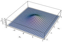
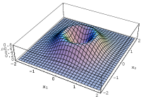
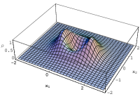
Figure 1: The profiles of the vortex solutions. $|\psi_{z}|^{2}$ is shown in the examples of (84) with $n=1$ (left) and $n=2$ (middle), and $f(z)=\frac{1}{z(z-1)}$ (right).

5 The super Schrödinger symmetry preserved by the vortices

The vortices found in the previous section are exact solutions to the BPS equations. In this section we study their supersymmetric properties and see how many of the non-relativistic supercharges are preserved by the BPS solutions. Our notations and terminology of the non-relativistic SUSY transformations follow [29]. We shall decompose the SUSY transformation parameters $\omega_{AB}$ and $\omega^{AB}$ using the basis $u_{\pm}$ in the same way as we did for the fermions:

$$\omega = \tilde{\omega}_{-}u_{+}+\tilde{\omega}_{+}u_{-}=\frac{1}{\sqrt{2}}\left(\begin{array}[]{c}\tilde{\omega}_{-}+\tilde{\omega}_{+}\\ -i\tilde{\omega}_{-}+i\tilde{\omega}_{+}\end{array}\right),$$ (95)

$$\tilde{\omega}^{AB}_{\pm} = (\tilde{\omega}_{\pm AB})^{\dagger}=\frac{1}{2}\epsilon^{ABCD}\tilde{\omega}_{\pm CD},$$ (96)

where $\epsilon^{1234}=\epsilon_{1234}=1$.

The super Schrödinger symmetry is generated by 14 components of supercharges. Ten of them are associated with kinematical SUSY, characterised by anti-commutation relations of the supercharges $\{Q_{K},Q^{\dagger}_{K}\}\sim{{\mathcal{M}}}/m$ where ${{\mathcal{M}}}$ is the total mass operator. The corresponding 10 SUSY parameters are

$$\left(\tilde{\omega}_{+\hat{A}\hat{B}},\;\;\tilde{\omega}_{-\check{A}\check{B}},\;\;\tilde{\omega}_{\pm\hat{A}\check{B}}\right).$$ (97)

Two of the other supercharge components belong to dynamical SUSY, characterised by supercharge commutator $\{Q_{D},Q^{\dagger}_{D}\}\sim H$, and their SUSY parameters are

$$\left(\tilde{\omega}_{-\hat{A}\hat{B}},\;\;\tilde{\omega}_{+\check{A}\check{B}}\right).$$ (98)

The two remaining components are associated with conformal SUSY.

The transformation rules for the kinematical SUSY are

$$\delta_{K}z^{\hat{A}} = \omega_{-}^{\hat{A}\hat{B}}\psi_{+\hat{B}}-\omega_{+}^{\hat{A}\check{B}}\psi_{-\check{B}},$$ (99)

$$\delta_{K}w^{\dagger\check{A}} = \omega_{-}^{\check{A}\hat{B}}\psi_{+\hat{B}}-\omega_{+}^{\check{A}\check{B}}\psi_{-\check{B}},$$ (100)

$$\delta_{K}\psi_{+\hat{A}} = -\omega_{+\hat{A}\hat{B}}z^{\hat{B}}+\omega_{+\hat{A}\check{B}}w^{\dagger\check{B}},$$ (101)

$$\delta_{K}\psi_{-\check{A}} = \omega_{-\check{A}\hat{B}}z^{\hat{B}}+\omega_{-\check{A}\check{B}}w^{\dagger\check{B}},$$ (102)

$$\delta_{K}A_{t} = \frac{\pi\hbar}{km}\left[z^{\hat{A}}\bar{\psi}_{+}^{\check{B}}\omega_{-\hat{A}\check{B}}+w^{\dagger\check{A}}\bar{\psi}_{+}^{\check{B}}\omega_{-\check{A}\check{B}}+z^{\hat{A}}\bar{\psi}_{-}^{\hat{B}}\omega_{+\hat{A}\hat{B}}+w^{\dagger\check{A}}\bar{\psi}_{-}^{\hat{B}}\omega_{+\check{A}\hat{B}}\right.$$ (103)

$$\qquad\left.+\omega_{-}^{\hat{A}\hat{B}}z^{\dagger}_{\hat{A}}\psi_{+\hat{B}}+\omega_{-}^{\check{A}\hat{B}}w_{\check{A}}\psi_{+\hat{B}}+\omega_{+}^{\hat{A}\check{B}}z^{\dagger}_{\hat{A}}\psi_{-\check{B}}+\omega_{+}^{\check{A}\check{B}}w_{\check{A}}\psi_{-\check{B}}\right],$$

$$\delta_{K}A_{+} = \frac{2\pi}{km}\left(w^{\dagger\check{A}}\bar{\psi}_{+}^{\check{B}}\omega_{+\check{A}\check{B}}+\omega_{+}^{\hat{A}\hat{B}}\psi_{+\hat{A}}z^{\dagger}_{\hat{B}}\right),$$ (104)

$$\delta_{K}A_{-} = \frac{2\pi}{km}\left(z^{\hat{A}}\bar{\psi}_{-}^{\hat{B}}\omega_{-\hat{A}\hat{B}}+\omega_{-}^{\check{A}\check{B}}\psi_{-\check{A}}w_{\check{B}}\right),$$ (105)

and the rules for the dynamical SUSY are

$$\delta_{D}z^{\hat{A}} = -\frac{i}{2m}\omega_{-}^{\hat{A}\hat{B}}D_{-}\psi_{+\hat{B}},$$ (106)

$$\delta_{D}w^{\dagger\check{A}} = \frac{i}{2m}\omega_{-}^{\check{A}\check{B}}D_{+}\psi_{-\check{B}},$$ (107)

$$\delta_{D}\psi_{+\hat{A}} = \frac{i}{2m}\omega_{-\hat{A}\hat{B}}D_{+}z^{\hat{B}},$$ (108)

$$\delta_{D}\psi_{-\check{A}} = -\frac{i}{2m}\omega_{+\check{A}\check{B}}D_{-}w^{\dagger\check{B}},$$ (109)

$$\delta_{D}A_{t} = \frac{i\pi\hbar}{2km^{2}}\left[-z^{\hat{A}}D_{+}\bar{\psi}_{-}^{\hat{B}}\omega_{-\hat{A}\hat{B}}-w^{\dagger\check{A}}D_{-}\bar{\psi}_{+}^{\check{B}}\omega_{+\check{A}\check{B}}\right.$$ (110)

$$\qquad\left.+\omega_{-}^{\hat{A}\hat{B}}w_{\check{A}}D_{+}\psi_{-\check{B}}+\omega_{+}^{\hat{A}\hat{B}}z^{\dagger}_{\hat{A}}D_{-}\psi_{+\hat{B}}\right],$$

$$\delta_{D}A_{\pm} = 0.$$ (111)

For the sake of brevity we have used in these expressions rescaled SUSY parameters

$$\left(\omega_{+\hat{A}\hat{B}},\omega_{-\check{A}\check{B}},\omega_{\pm\hat{A}\check{B}}\right) \equiv \sqrt{\frac{2mc}{\hbar}}\left(\tilde{\omega}_{+\hat{A}\hat{B}},\tilde{\omega}_{-\check{A}\check{B}},\tilde{\omega}_{\pm\hat{A}\check{B}}\right),$$ (112)

$$\left(\omega_{+}^{\check{A}\check{B}},\omega_{-}^{\hat{A}\hat{B}},\omega_{\pm}^{\hat{A}\check{B}}\right) \equiv \sqrt{\frac{2mc}{\hbar}}\left(\tilde{\omega}_{+}^{\check{A}\check{B}},\tilde{\omega}_{-}^{\hat{A}\hat{B}},\tilde{\omega}_{\pm}^{\hat{A}\check{B}}\right),$$ (113)

and

$$\left(\omega_{-\hat{A}\hat{B}},\omega_{+\check{A}\check{B}}\right) \equiv \sqrt{\frac{2m\hbar}{c}}\left(\tilde{\omega}_{-\hat{A}\hat{B}},\tilde{\omega}_{+\check{A}\check{B}}\right),$$ (114)

$$\left(\omega_{-}^{\check{A}\check{B}},\omega_{+}^{\hat{A}\hat{B}}\right) \equiv \sqrt{\frac{2m\hbar}{c}}\left(\tilde{\omega}_{-}^{\check{A}\check{B}},\tilde{\omega}_{+}^{\hat{A}\hat{B}}\right).$$ (115)

Dimensions of these new parameters are

$$[\omega_{+\hat{A}\hat{B}}]=[\omega_{-\check{A}\check{B}}]=[\omega_{\pm\hat{A}\check{B}}]=[\omega_{+}^{\check{A}\check{B}}]=[\omega_{-}^{\hat{A}\check{B}}]=[\omega_{\pm}^{\hat{A}\check{B}}]=1,$$ (116)

$$[\omega_{-\hat{A}\hat{B}}]=[\omega_{+\check{A}\check{B}}]=[\omega_{-}^{\check{A}\check{B}}]=[\omega_{+}^{\hat{A}\hat{B}}]=ML.$$ (117)

We sketch derivation of the non-relativistic SUSY transformation formulae in the Appendix.

Let us first consider the BPS-I vortices, which are solutions to the BPS equations

$$w^{\dagger\check{A}}=0,\quad D_{-}z^{\hat{A}}=0.$$ (118)

Applying these conditions to the fermion transformation rules $\delta\psi$, we have

$$\delta_{K}\psi_{+\hat{A}} = -\omega_{+\hat{A}\hat{B}}z^{\hat{B}},$$ (119)

$$\delta_{D}\psi_{+\hat{A}} = \frac{i}{2m}\omega_{-\hat{A}\hat{B}}D_{+}z^{\hat{B}},$$ (120)

$$\delta_{K}\psi_{-\check{A}} = +\omega_{-\check{A}\hat{B}}z^{\hat{B}},$$ (121)

$$\delta_{D}\psi_{-\check{A}} = 0,$$ (122)

hence the conditions $\delta\psi=0$ imply $\omega_{+\hat{A}\hat{B}}=\omega_{-\hat{A}\hat{B}}=\omega_{-\check{A}\hat{B}}=0$. This means that the BPS-I solutions break 5 kinematical and 1 dynamical SUSYs.

For the BPS-II solutions the BPS equations are

$$z^{\hat{A}}=0,\quad D_{+}w^{\dagger\check{A}}=0,$$ (123)

and the transformation rules become

$$\delta_{K}\psi_{+\hat{A}} = \omega_{+\hat{A}\check{B}}w^{\dagger\check{B}},$$ (124)

$$\delta_{D}\psi_{+\hat{A}} = 0,$$ (125)

$$\delta_{K}\psi_{-\check{A}} = \omega_{-\check{A}\check{B}}w^{\dagger\check{B}},$$ (126)

$$\delta_{D}\psi_{-\check{A}} = -\frac{i}{2m}\omega_{+\check{A}\check{B}}D_{-}w^{\dagger\check{B}}.$$ (127)

The conditions $\delta\psi=0$ then give $\omega_{+\hat{A}\check{B}}=\omega_{-\check{A}\check{B}}=\omega_{+\check{A}\check{B}}=0$ and we see that the BPS-II solutions also break 5 kinematical and 1 dynamical SUSYs.

The properties of the vortex solutions associated with the the conformal SUSY can be inferred from the fact that the conformal supercharge $S$ is written as a commutator of the special conformal generator $K$ and the dynamical supercharge $Q_{D}$ [34, 28, 29],

$$S=i[K,Q_{D}].$$ (128)

Using the dynamical SUSY transformation rules (108), (109) we see that under the conformal SUSY $\delta_{S}\psi_{+\hat{A}}\sim\xi_{\hat{A}\hat{B}}z^{\hat{B}}$ and $\delta_{S}\psi_{-\check{A}}\sim\xi_{\check{A}\check{B}}w^{{\dagger}\check{B}}$. The former vanishes for the BPS-II conditions (123) whereas the latter vanishes for the BPS-I conditions (118). We may thus conclude that the BPS-I and BPS-II both preserve half of the conformal SUSY. Note that once we turn on both $z^{\hat{A}}$ and $w^{\dagger\check{A}}$, the BPS equations break all the SUSYs in general and hence there would be only trivial solution $z^{\hat{A}}=w^{\dagger\check{A}}=0$. We summarize the results in table 1.

Type of	Kinematical				Dynamical		Conformal
SUSY	$\omega_{+\hat{A}\check{B}}$	$\omega_{+\hat{A}\hat{B}}$	$\omega_{-\check{A}\check{B}}$	$\omega_{-\check{A}\hat{B}}$	$\omega_{-\hat{A}\hat{B}}$	$\omega_{+\check{A}\check{B}}$	$\xi_{\hat{A}\hat{B}}$	$\xi_{\check{A}\check{B}}$
BPS I	$\bigcirc$	$\times$	$\bigcirc$	$\times$	$\times$	$\bigcirc$	$\times$	$\bigcirc$
BPS II	$\times$	$\bigcirc$	$\times$	$\bigcirc$	$\bigcirc$	$\times$	$\bigcirc$	$\times$

Table 1: Broken and preserved SUSYs for our vortex solutions BPS-I and BPS-II. Here $\bigcirc$ for preserved, and $\times$ for broken SUSYs.

6 Discussions

In this paper we studied vortex solutions in the non-relativistic ABJM model and discussed the non-relativistic SUSY they preserve. The ABJM model is a particularly interesting type of Chern-Simons-matter theory as its gravitational dual is well understood and its non-relativistic limit is also expected to have a gravitational dual through a non-relativistic version of AdS/CFT correspondence [23, 24, 25, 26, 27]. We obtained exact solutions to the BPS equations and showed that these vortices preserve half of the 10 kinematical, 2 dynamical and 2 conformal SUSYs. The solutions discussed in this paper are related to those of the Jackiw-Pi model. In fact, the correspondence can be seen at the Lagrangian level. Let us take the BPS-I ansatz for example: setting $w_{\check{A}}=0$ and assuming the fuzzy $S^{3}$ configuration,

$$z^{\hat{A}}=\psi S^{I},\quad A_{\mu}=a_{\mu}S^{I}S^{\dagger}_{I},\quad\hat{A}_{\mu}=a_{\mu}S^{\dagger}_{I}S^{I},$$ (129)

the non-relativistic ABJM model Lagrangian (43) reduces to

$$\mathcal{L}^{\rm NR,bos}_{\rm ABJM}=N(N-1)\mathcal{L}_{\rm JP},$$ (130)

where

$${{\mathcal{L}}}_{\rm JP}=\frac{k}{4\pi}\epsilon^{\mu\nu\lambda}a_{\mu}\partial_{\nu}a_{\lambda}+\frac{i\hbar}{2}(-\psi\mathcal{D}_{t}\bar{\psi}+\bar{\psi}\mathcal{D}_{t}\psi)-\frac{\hbar^{2}}{2m}|\mathcal{D}_{i}\psi|^{2}+\frac{\pi\hbar^{2}}{km}(\psi\bar{\psi})^{2},$$ (131)

is identified as the Lagrangian of the Jackiw-Pi model [31]. We note that the fuzzy $S^{3}$ sphere ansatz is essential in this correspondence, and the correspondence holds only for $N\geq 2$. The Jackiw-Pi model gives abelian vortices, whereas the gauge fields of the ABJM model (of $N\geq 2$) are non-abelian. We may say that the abelian vortices are embedded in the non-relativistic ABJM model, with the non-abelian nature of the ABJM gauge fields converted into the fuzziness of the $S^{3}$ part and the numerical factor of (130).

While our solutions may be considered as an embedding of the abelian Jackiw-Pi vortices, it is not obvious from this fact alone how many of the non-relativistic 14 SUSYs are preserved by the BPS solutions. The Jackiw-Pi model $\mathcal{L}_{JP}$, which is the non-relativistic limit of the $\mathcal{N}=2$ abelian Chern-Simons-Higgs model [30], does not exhibit 14 SUSYs but keeps only a part of them. This means that in order to see the full structure of the unbroken SUSY kept by the vortex solutions, it is necessary to analyse the BPS equation (78) derived from the original non-relativistic ABJM model, not the effective description (130), (131). One of our motivations to look for vortex solutions in the non-relativistic ABJM model arose from their potential importance in holographic descriptions of $(1+2)$ dimensional condensed matter systems. The structure of the preserved SUSYs is important for determining the corresponding solutions in the gravity side. It would be interesting to find a solution that preserves 7 Schrödinger SUSYs in the eleven dimensional gravity dual.

Let us comment on more realistic models for condensed matter physics. Physically interesting problems such as superconductivity and quantum Hall effect involve external fields, and the parity of the systems is accordingly broken. While the Jackiw-Pi vortex solutions that we described in this paper do not involve external fields, a straightforward modification to include external fields is known once the Lagrangian is suitably modified. For example, let us add an additional term to the ABJM Lagrangian,

$$\delta{{\mathcal{L}}}=\mathop{\rm Tr}\left[F_{12}Z^{\hat{A}}Z^{\dagger}_{\hat{A}}-\hat{F}_{12}Z^{\dagger}_{\hat{A}}Z^{\hat{A}}\right].$$ (132)

With the fuzzy $S^{3}$ configuration

$$F_{12}=BS^{I}S^{\dagger}_{I},\qquad\hat{F}_{12}=BS^{{\dagger}}_{I}S^{I},$$ (133)

together with the BPS-I ansatz, the Hamiltonian acquires an additional term proportional to $N(N-1)\frac{\hbar}{2m}B|\psi_{z}|^{2}$. It is then possible to modify the vortex solutions to include the external fields following [35]. It is interesting to see whether it is possible to accommodate more realistic models such as the Zhang-Hansson-Kivelson model [36] of the quantum Hall effect.

Finally, it is also an interesting question whether the model allows other types of solitonic solutions, such as an embedding of non-abelian vortices, solutions with less supersymmetry, time-dependent solutions and so on. For embedding non-abelian solutions, once one assumes an ansatz $A_{\mu}=\hat{A}_{\mu}$, the bi-fundamental scalar fields can be effectively treated as adjoint matter fields. It would be interesting to see if it is possible to embed the non-Abelian solutions of the Toda-type [37]. Finding more general solutions requires further study. Determination of the complete moduli space of the solutions, in particular its relation to the broken SUSY structure, and clarification of the string theoretical origin of additional terms like (132) are also important problems. We hope to come back to these issues in near future.

Acknowledgements

We acknowledge helpful discussions with Claus Montonen, Seiji Terashima, Koji Hashimoto, Esko Keski-Vakkuri, Sean Nowling and Patta Yogendran. This work is in part supported by JSPS-Academy of Finland bilateral scientist exchange programme (SS) and the Academy of Finland Finnish-Japanese Core Programme Grant No. 112420 (SK).

Appendix A The Non-relativistic supersymmetry

In this appendix we describe how the non-relativistic SUSY transformation rules (99)-(111) arise in the non-relativistic limit of the ${{\mathcal{N}}}=6$ mass-deformed SUSY transformations. This is accomplished by decomposing the relativistic fields into non-relativistic particle and antiparticle parts, dropping the antiparticle part, and expand for large $c$ and $m$. Then the leading terms are identified as the kinematical and the next-to-leading as the dynamical SUSY transformation terms. See [28, 29, 34] for further details, and [38, 39] for related work on the Schrödinger and super Schrödinger algebras.

We use the following conventions: the 3-dimensional gamma matrices are

$$(\gamma^{\mu})_{\alpha}{}^{\beta}=(i\sigma_{2},\sigma_{1},\sigma_{3}),\quad\{\gamma^{\mu},\gamma^{\nu}\}=2\eta^{\mu\nu}.$$ (134)

A spinor product is related to a matrix product as

$$\Psi^{\dagger\alpha}\Psi_{\alpha}=-\mathbf{\Psi}^{\dagger}\gamma^{0}\mathbf{\Psi},$$ (135)

where $\mathbf{\Psi}$ is a $2\times 1$ matrix (vector) and the dagger in the right hand side is interpreted as the matrix adjoint. In the following, we interpret $\Psi$ as the two component vector $\mathbf{\Psi}$. The spinor indices are raised and lowered as

$$\theta^{\alpha}=\epsilon^{\alpha\beta}\theta_{\beta},\quad\theta_{\alpha}=\epsilon_{\alpha\beta}\theta^{\beta},\quad\epsilon^{12}=-\epsilon_{12}=1.$$ (136)

The standard position of spinor contraction is

$$\theta\chi=\theta^{\alpha}\chi_{\alpha}=-\mathbf{\theta}^{t}\gamma^{0}\mathbf{\chi}.$$ (137)

A.1 The scalar part

Let us start from the scalar part and consider the transformation $\delta Y^{A}=i\omega^{AB}\Psi_{B}$. Using the fermion decomposition (55) we may write

$$(\omega^{AB})^{\alpha}(\Psi_{B})_{\alpha} = -\omega^{AB}\gamma^{0}\Psi_{B}$$ (138)

$$= -\sqrt{\hbar c}i(\tilde{\omega}_{-}^{AB}\psi_{+B}-\tilde{\omega}_{+}^{AB}\psi_{-B})e^{-i\frac{mc^{2}}{\hbar}t}.$$

Decomposing the scalar field as

$$Y^{A}=\frac{\hbar}{\sqrt{2m}}y^{A}e^{-\frac{mc^{2}}{\hbar}t}+\textrm{(anti particle)},$$ (139)

and dropping the antiparticle part, the first two components of the SUSY transformation becomes

$$\delta z^{\hat{A}} = \frac{\sqrt{2m\hbar c}}{\hbar}\left(\tilde{\omega}_{-}^{\hat{A}\hat{B}}\psi_{+\hat{B}}+\tilde{\omega}_{-}^{\hat{A}\check{B}}\psi_{+\check{B}}-\tilde{\omega}_{+}^{\hat{A}\hat{B}}\psi_{-\hat{B}}-\tilde{\omega}_{+}^{\hat{A}\check{B}}\psi_{-\check{B}}\right)$$ (140)

$$= \frac{\sqrt{2m\hbar c}}{\hbar}\left(\tilde{\omega}_{-}^{\hat{A}\hat{B}}\psi_{+\hat{B}}+\frac{i\hbar}{2mc}\tilde{\omega}_{-}^{\hat{A}\check{B}}D_{+}\psi_{-\check{B}}-\frac{i\hbar}{2mc}\tilde{\omega}_{+}^{\hat{A}\hat{B}}D_{-}\psi_{+\hat{B}}-\tilde{\omega}_{+}^{\hat{A}\check{B}}\psi_{-\check{B}}\right)$$

$$\qquad+\textrm{ (higher order terms)}.$$

We have used the Dirac equations (58), (59) to go to the second line. From the leading order we find (using the rescaled parameters),

$$\delta_{K}z^{\hat{A}}=\omega_{-}^{\hat{A}\hat{B}}\psi_{+\hat{B}}-\omega_{+}^{\hat{A}\check{B}}\psi_{-\check{B}},$$ (141)

and from the next-to-leading order,

$$\delta_{D}z^{\hat{A}}=-\frac{i}{2m}\omega_{-}^{\hat{A}\hat{B}}D_{-}\psi_{+\hat{B}}.$$ (142)

From the other components we similarly find

$$\delta_{K}w^{\dagger\check{A}} = \omega_{-}^{\check{A}\hat{B}}\psi_{+\hat{B}}-\omega_{+}^{\check{A}\check{B}}\psi_{-\check{B}},$$ (143)

$$\delta_{D}w^{\dagger\check{A}} = \frac{i}{2m}\omega_{-}^{\check{A}\check{B}}D_{+}\psi_{-\check{B}}.$$ (144)

A.2 The fermion part

Next we consider the transformation of the fermion. The first term on the RHS of the SUSY transformation can be written upon particle-antiparticle decomposition (and neglecting the antiparticle) as

$$\gamma^{\mu}\omega_{AB}D_{\mu}Y^{B}$$

$$\quad=-i\frac{mc}{\sqrt{2m}}\gamma^{0}\omega_{AB}y^{B}e^{-\frac{mc^{2}}{\hbar}t}+\frac{1}{\sqrt{2m}}\frac{\hbar}{c}\gamma^{0}\omega_{AB}D_{t}y^{B}e^{-\frac{mc^{2}}{\hbar}t}+\frac{\hbar}{\sqrt{2m}}\gamma^{i}\omega_{AB}D_{i}y^{B}e^{-\frac{mc^{2}}{\hbar}t}$$

$$\quad=\left(\begin{array}[]{c}\frac{mc}{\hbar}(\tilde{\omega}_{+AB}-\tilde{\omega}_{-AB})y^{B}+\frac{1}{c}(i\tilde{\omega}_{+AB}-i\tilde{\omega}_{-AB})D_{t}y^{B}+i\tilde{\omega}_{+AB}D_{-}y^{B}-i\tilde{\omega}_{-AB}D_{+}y^{B}\\ \frac{mc}{\hbar}(i\tilde{\omega}_{+AB}+i\tilde{\omega}_{-AB})y^{B}-\frac{1}{c}(\tilde{\omega}_{+AB}+\tilde{\omega}_{-AB})D_{t}y^{B}+\tilde{\omega}_{+AB}D_{-}y^{B}+\tilde{\omega}_{-AB}D_{+}y^{B}\end{array}\right)$$ (147)

$$\qquad\qquad\qquad\qquad\times\frac{\hbar}{2\sqrt{m}}e^{-i\frac{mc^{2}}{\hbar}t}.$$ (148)

The $D_{t}y^{B}$ terms are subleading and can be dropped. The mass independent part in the second term on the RHS is also subleading. The mass-dependent term gives non-trivial contributions,

$$\frac{mc}{\hbar}Y^{C}\omega_{\hat{A}C}=\frac{c}{2}\sqrt{m}\left(\begin{array}[]{cc}z^{\hat{B}}\tilde{\omega}_{-\hat{A}\hat{B}}+w^{{\dagger}\check{B}}\tilde{\omega}_{-\hat{A}\check{B}}+z^{\hat{B}}\tilde{\omega}_{+\hat{A}\hat{B}}+w^{{\dagger}\check{B}}\tilde{\omega}_{+\hat{A}\check{B}}\\ -iz^{\hat{B}}\tilde{\omega}_{-\hat{A}\hat{B}}-iw^{{\dagger}\check{B}}\tilde{\omega}_{-\hat{A}\check{B}}+iz^{\hat{B}}\tilde{\omega}_{+\hat{A}\hat{B}}+iw^{{\dagger}\check{B}}\tilde{\omega}_{+\hat{A}\check{B}}\end{array}\right).$$ (149)

As the fermion transformations decompose as

$$\delta\Psi_{A}=\frac{1}{\sqrt{2}}\sqrt{\hbar c}\left(\begin{array}[]{c}\delta\psi_{-A}+\delta\psi_{+A}\\ -i\delta\psi_{-A}+i\delta\psi_{+A}\end{array}\right)e^{-i\frac{mc^{2}}{\hbar}t},$$ (152)

we find

$$\delta\psi_{-\hat{A}}+\delta\psi_{+\hat{A}} = +i\frac{mc}{\sqrt{2m\hbar c}}\left(-i\tilde{\omega}_{-\hat{A}\hat{B}}+i\tilde{\omega}_{+\hat{A}\hat{B}}\right)z^{\hat{B}}+i\frac{mc}{\sqrt{2m\hbar c}}\left(-i\tilde{\omega}_{-\hat{A}\check{B}}+i\tilde{\omega}_{+\hat{A}\check{B}}\right)w^{\dagger\check{B}}$$ (153)

$$-\frac{\hbar}{\sqrt{2m\hbar c}}\left(-i\tilde{\omega}_{-\hat{A}\hat{B}}D_{+}z^{\hat{B}}-i\tilde{\omega}_{-\hat{A}\check{B}}D_{+}w^{\dagger\check{B}}+i\tilde{\omega}_{+\hat{A}\hat{B}}D_{-}z^{\hat{B}}+i\tilde{\omega}_{+\hat{A}\check{B}}D_{-}w^{\dagger\check{B}}\right)$$

$$-\frac{mc}{\hbar}\frac{\hbar}{\sqrt{2m\hbar c}}\left(z^{\hat{B}}\tilde{\omega}_{-\hat{A}\hat{B}}+w^{\dagger\check{B}}\tilde{\omega}_{-\hat{A}\check{B}}+z^{\hat{B}}\tilde{\omega}_{+\hat{A}\hat{B}}+w^{\dagger\check{B}}\tilde{\omega}_{+\hat{A}\check{B}}\right),$$

$$-i\delta\psi_{-\hat{A}}+i\delta\psi_{+\hat{A}} = +i\frac{mc}{\sqrt{2m\hbar c}}\left(-\tilde{\omega}_{-\hat{A}\hat{B}}-\tilde{\omega}_{+\hat{A}\hat{B}}\right)z^{\hat{B}}+i\frac{mc}{\sqrt{2m\hbar c}}\left(-\tilde{\omega}_{-\hat{A}\check{B}}-\tilde{\omega}_{+\hat{A}\check{B}}\right)w^{\dagger\check{B}}$$ (154)

$$-\frac{\hbar}{\sqrt{2m\hbar c}}\left(\tilde{\omega}_{-\hat{A}\hat{B}}D_{+}z^{\hat{B}}+\tilde{\omega}_{-\hat{A}\check{B}}D_{+}w^{\dagger\check{B}}+\tilde{\omega}_{+\hat{A}\hat{B}}D_{-}z^{\hat{B}}+\tilde{\omega}_{+\hat{A}\check{B}}D_{-}w^{\dagger\check{B}}\right)$$

$$-\frac{mc}{\hbar}\frac{\hbar}{\sqrt{2m\hbar c}}\left(-iz^{\hat{B}}\tilde{\omega}_{-\hat{A}\hat{B}}-iw^{\dagger\check{B}}\tilde{\omega}_{-\hat{A}\check{B}}+iz^{\hat{B}}\tilde{\omega}_{+\hat{A}\hat{B}}+iw^{\dagger\check{B}}\tilde{\omega}_{+\hat{A}\check{B}}\right).$$

Because of the Dirac equations (58), (59), $\delta\psi_{-\hat{A}}$ on the LHS is subleading. Then in terms of the rescaled SUSY parameters we obtain the kinematical $\delta_{K}$ and dynamical $\delta_{D}$ SUSY transformations

$$\delta_{K}\psi_{+\hat{A}} = -\omega_{+\hat{A}\hat{B}}z^{\hat{B}}+\omega_{+\hat{A}\check{B}}w^{\dagger\check{B}},$$ (155)

$$\delta_{D}\psi_{+\hat{A}} = \frac{i}{2m}\omega_{-\hat{A}\hat{B}}D_{+}z^{\hat{B}}.$$ (156)

Similarly,

$$\delta\psi_{-\check{A}}+\delta\psi_{+\check{A}} = \frac{i\hbar}{\sqrt{2m\hbar c}}\left(\tilde{\omega}_{-\check{A}\hat{B}}D_{+}z^{\hat{B}}+\tilde{\omega}_{-\check{A}\check{B}}D_{+}w^{\dagger\check{B}}-\tilde{\omega}_{+\check{A}\hat{B}}D_{-}z^{\hat{B}}-\tilde{\omega}_{+\check{A}\check{B}}D_{-}w^{\dagger\check{B}}\right)$$ (157)

$$+\frac{2mc}{\sqrt{2m\hbar c}}\left(\tilde{\omega}_{-\check{A}\hat{B}}z^{\hat{B}}+\tilde{\omega}_{-\check{A}\check{B}}w^{\dagger\check{B}}\right),$$

$$-i\delta\psi_{-\check{A}}+i\delta\psi_{+\check{A}} = -\frac{\hbar}{\sqrt{2m\hbar c}}\left(\tilde{\omega}_{\check{A}\hat{B}}D_{+}z^{\hat{B}}+\tilde{\omega}_{-\check{A}\check{B}}D_{+}w^{\dagger\check{B}}+\tilde{\omega}_{+\check{A}\hat{B}}D_{-}z^{\hat{B}}+\tilde{\omega}_{+\check{A}\check{B}}D_{-}w^{\dagger\check{B}}\right)$$ (158)

$$-i\frac{2mc}{\sqrt{2m\hbar c}}\left(\tilde{\omega}_{-\check{A}\hat{B}}z^{\hat{B}}+\tilde{\omega}_{-\check{A}\check{B}}w^{\dagger\check{B}}\right),$$

and again due to the Dirac equations (58), (59) we may drop $\delta\psi_{+\check{A}}$ on the LHS, leading to

$$\delta_{K}\psi_{-\check{A}} = \omega_{-\check{A}\hat{B}}z^{\hat{B}}+\omega_{-\check{A}\check{B}}w^{\dagger\check{B}},$$ (159)

$$\delta_{D}\psi_{-\check{A}} = -\frac{i}{2m}\omega_{+\check{A}\check{B}}D_{-}w^{\dagger\check{B}}.$$ (160)

A.3 The gauge field part

Finally we consider the gauge field part. Note that the temporal and the spatial parts of the relativistic SUSY transformation formula come with different powers of $c$:

$$\delta A_{t} = +\frac{2\pi}{k\hbar}\left(Y^{A}\Psi^{\dagger B}\gamma^{0}\omega_{AB}+\omega^{AB}\gamma^{0}\Psi_{A}Y^{\dagger}_{B}\right),$$ (161)

$$\delta A_{\pm} = -\frac{2\pi}{k\hbar c}\left(Y^{A}\Psi^{\dagger B}\gamma^{\pm}\omega_{AB}+\omega^{AB}\gamma^{i}\Psi_{A}Y^{\dagger}_{B}\right),$$ (162)

where

$$\gamma^{\pm}\equiv\gamma^{1}\pm i\gamma^{2}=\left(\begin{array}[]{cc}\pm i&1\\ 1&\mp i\end{array}\right).$$ (165)

Upon non-relativistic decomposition of the fields the temporal part becomes

$$\delta A_{t} = \frac{2\pi}{k}\sqrt{\frac{\hbar c}{2m}}\left[-\frac{i\hbar}{2mc}z^{\hat{A}}D_{+}\bar{\psi}_{-}^{\hat{B}}\tilde{\omega}_{-\hat{A}\hat{B}}-\frac{i\hbar}{2mc}w^{\dagger\check{A}}D_{+}\bar{\psi}_{-}^{\hat{B}}\tilde{\omega}_{-\check{A}\hat{B}}+z^{\hat{A}}\bar{\psi}_{+}^{\check{B}}\tilde{\omega}_{-\hat{A}\check{B}}+w^{\dagger\check{A}}\bar{\psi}_{+}^{\check{B}}\tilde{\omega}_{-\check{A}\check{B}}\right.$$ (166)

$$\qquad+z^{\hat{A}}\bar{\psi}_{-}^{\hat{B}}\psi_{+\hat{A}\hat{B}}+w^{\dagger\check{A}}\bar{\psi}_{-}^{\hat{B}}\tilde{\omega}_{+\check{A}\hat{B}}-\frac{i\hbar}{2mc}z^{\hat{A}}D_{-}\bar{\psi}_{+}^{\check{B}}\tilde{\omega}_{+\hat{A}\check{B}}-\frac{i\hbar}{2mc}w^{\dagger\check{A}}D_{-}\bar{\psi}_{+}^{\check{B}}\tilde{\omega}_{+\check{A}\check{B}}$$

$$\qquad+\tilde{\omega}_{-}^{\hat{A}\hat{B}}z^{\dagger}_{\hat{A}}\psi_{+\hat{B}}+\tilde{\omega}_{-}^{\check{A}\hat{B}}w_{\check{A}}\psi_{+\hat{B}}+\frac{i\hbar}{2mc}\tilde{\omega}_{-}^{\hat{A}\check{B}}z^{\dagger}_{\hat{A}}D_{+}\psi_{-\check{B}}+\frac{i\hbar}{2mc}\tilde{\omega}_{-}^{\check{A}\check{B}}w_{\check{A}}D_{+}\psi_{-\check{B}}$$

$$\qquad\left.+\frac{i\hbar}{2mc}\tilde{\omega}_{+}^{\hat{A}\hat{B}}z^{\dagger}_{\hat{A}}D_{-}\psi_{+\hat{B}}+\frac{i\hbar}{2mc}\tilde{\omega}_{+}^{\check{A}\hat{B}}w_{\check{A}}D_{-}\psi_{+\hat{B}}+\tilde{\omega}_{+}^{\hat{A}\check{B}}z^{\dagger}_{\hat{A}}\psi_{-\check{B}}+\tilde{\omega}_{+}^{\check{A}\check{B}}w_{\check{A}}\psi_{-\check{B}}\right]$$

$$\qquad+\textrm{(higher order terms)}.$$

Using the rescaled SUSY parameters we obtain

$$\delta_{K}A_{t} = \frac{\pi\hbar}{km}\left[z^{\hat{A}}\bar{\psi}_{+}^{\check{B}}\omega_{-\hat{A}\check{B}}+w^{\dagger\check{A}}\bar{\psi}_{+}^{\check{B}}\omega_{-\check{A}\check{B}}+z^{\hat{A}}\bar{\psi}_{-}^{\hat{B}}\omega_{+\hat{A}\hat{B}}+w^{\dagger\check{A}}\bar{\psi}_{-}^{\hat{B}}\omega_{+\check{A}\hat{B}}\right.$$ (167)

$$\qquad\left.+\omega_{-}^{\hat{A}\hat{B}}z^{\dagger}_{\hat{A}}\psi_{+\hat{B}}+\omega_{-}^{\check{A}\hat{B}}w_{\check{A}}\psi_{+\hat{B}}+\omega_{+}^{\hat{A}\check{B}}z^{\dagger}_{\hat{A}}\psi_{-\check{B}}+\omega_{+}^{\check{A}\check{B}}w_{\check{A}}\psi_{-\check{B}}\right],$$

$$\delta_{D}A_{t} = \frac{i\pi\hbar}{2km^{2}}\left[-z^{\hat{A}}D_{+}\bar{\psi}_{-}^{\hat{B}}\omega_{-\hat{A}\hat{B}}-w^{\dagger\check{A}}D_{-}\bar{\psi}_{+}^{\check{B}}\omega_{+\check{A}\check{B}}+\omega_{-}^{\hat{A}\hat{B}}w_{\check{A}}D_{+}\psi_{-\check{B}}+\omega_{+}^{\hat{A}\hat{B}}z^{\dagger}_{\hat{A}}D_{-}\psi_{+\hat{B}}\right].$$

The spatial part of the transformation formula can be found similarly. From

$$\delta A_{+} = \frac{4\pi}{kc}\sqrt{\frac{\hbar c}{2m}}\left[-\frac{i\hbar}{2mc}z^{\hat{A}}D_{+}\bar{\psi}_{-}^{\hat{B}}\tilde{\omega}_{+\hat{A}\hat{B}}-\frac{i\hbar}{2mc}w^{\dagger\check{A}}D_{+}\bar{\psi}_{-}^{\hat{B}}\tilde{\omega}_{+\check{A}\hat{B}}+z^{\hat{A}}\bar{\psi}_{+}^{\check{B}}\tilde{\omega}_{+\hat{A}\check{B}}+w^{\dagger\check{A}}\bar{\psi}_{+}^{\check{B}}\tilde{\omega}_{+\check{A}\check{B}}\right.$$ (169)

$$\qquad\qquad\left.+\tilde{\omega}_{+}^{\hat{A}\hat{B}}\psi_{+\hat{A}}z^{\dagger}_{\hat{B}}+\tilde{\omega}_{+}^{\hat{A}\check{B}}\psi_{+\hat{A}}w_{\check{B}}+\frac{i\hbar}{2mc}\tilde{\omega}_{+}^{\check{A}\hat{B}}D_{+}\psi_{-\check{A}}z^{\dagger}_{\hat{B}}+\frac{i\hbar}{2mc}\tilde{\omega}_{+}^{\check{A}\check{B}}D_{+}\psi_{-\check{A}}w_{\check{B}}\right]$$

$$\qquad+\textrm{(higher order terms)},$$

we obtain

$$\delta_{K}A_{+} = \frac{2\pi}{km}\left(w^{\dagger\check{A}}\bar{\psi}_{+}^{\check{B}}\omega_{+\check{A}\check{B}}+\omega_{+}^{\hat{A}\hat{B}}\psi_{+\hat{A}}z^{\dagger}_{\hat{B}}\right),$$ (170)

$$\delta_{D}A_{+} = 0,$$ (171)

and from

$$\delta A_{-} = \frac{4\pi}{kc}\sqrt{\frac{\hbar c}{2m}}\left[z^{\hat{A}}\bar{\psi}_{-}^{\hat{B}}\tilde{\omega}_{-\hat{A}\hat{B}}+w^{\dagger\check{A}}\bar{\psi}_{-}^{\hat{B}}\tilde{\omega}_{-\check{A}\hat{B}}-\frac{i\hbar}{2mc}z^{\hat{A}}D_{-}\bar{\psi}_{+}^{\check{B}}\tilde{\omega}_{-\hat{A}\check{B}}-\frac{i\hbar}{2mc}w^{\dagger\check{A}}D_{-}\bar{\psi}_{+}^{\check{B}}\tilde{\omega}_{-\check{A}\check{B}}\right.$$ (172)

$$\qquad\qquad\left.+\frac{i\hbar}{2mc}\tilde{\omega}_{-}^{\hat{A}\hat{B}}D_{-}\psi_{+\hat{A}}z^{\dagger}_{\hat{B}}+\frac{i\hbar}{2mc}\tilde{\omega}_{-}^{\hat{A}\check{B}}D_{-}\psi_{+\hat{A}}w_{\check{B}}+\tilde{\omega}_{-}^{\check{A}\hat{B}}\psi_{-\check{A}}z^{\dagger}_{\hat{B}}+\tilde{\omega}_{-}^{\check{A}\check{B}}\psi_{-\check{A}}w_{\check{B}}\right]$$

$$\qquad+\textrm{(higher order terms)},$$

we have

$$\delta_{K}A_{-} = \frac{2\pi}{km}\left(z^{\hat{A}}\bar{\psi}_{-}^{\hat{B}}\omega_{-\hat{A}\hat{B}}+\omega_{-}^{\check{A}\check{B}}\psi_{-\check{A}}w_{\check{B}}\right),$$ (173)

$$\delta_{D}A_{-} = 0.$$ (174)

References

- [1] J. Bagger and N. Lambert, Modeling multiple M2’s, Phys. Rev. D75 (2007) 045020, [hep-th/0611108].
- [2] J. Bagger and N. Lambert, Gauge Symmetry and Supersymmetry of Multiple M2-Branes, Phys. Rev. D77 (2008) 065008, [0711.0955].
- [3] J. Bagger and N. Lambert, Comments On Multiple M2-branes, JHEP 02 (2008) 105, [0712.3738].
- [4] A. Gustavsson, Algebraic structures on parallel M2-branes, Nucl. Phys. B811 (2009) 66–76, [0709.1260].
- [5] A. Gustavsson, Selfdual strings and loop space Nahm equations, JHEP 04 (2008) 083, [0802.3456].
- [6] O. Aharony, O. Bergman, D. L. Jafferis, and J. Maldacena, N=6 superconformal Chern-Simons-matter theories, M2-branes and their gravity duals, JHEP 10 (2008) 091, [0806.1218].
- [7] M. Benna, I. Klebanov, T. Klose, and M. Smedback, Superconformal Chern-Simons Theories and Correspondence, JHEP 09 (2008) 072, [0806.1519].
- [8] S. Terashima, On M5-branes in N=6 Membrane Action, JHEP 08 (2008) 080, [0807.0197].
- [9] K. Hanaki and H. Lin, M2-M5 Systems in N=6 Chern-Simons Theory, JHEP 09 (2008) 067, [0807.2074].
- [10] M. Arai, C. Montonen, and S. Sasaki, Vortices, Q-balls and Domain Walls on Dielectric M2- branes, JHEP 03 (2009) 119, [0812.4437].
- [11] T. Fujimori, K. Iwasaki, Y. Kobayashi, and S. Sasaki, Time-dependent and Non-BPS Solutions in N=6 Superconformal Chern-Simons Theory, JHEP 12 (2008) 023, [0809.4778].
- [12] C. Krishnan and C. Maccaferri, Membranes on Calibrations, JHEP 07 (2008) 005, [0805.3125].
- [13] J. Kim and B.-H. Lee, Abelian Vortex in Bagger-Lambert-Gustavsson Theory, JHEP 01 (2009) 001, [0810.3091].
- [14] I. Jeon, J. Kim, B.-H. Lee, J.-H. Park, and N. Kim, M-brane bound states and the supersymmetry of BPS solutions in the Bagger-Lambert theory, 0809.0856.
- [15] I. Jeon, J. Kim, N. Kim, S.-W. Kim, and J.-H. Park, Classification of the BPS states in Bagger-Lambert Theory, JHEP 07 (2008) 056, [0805.3236].
- [16] G. Bonelli, A. Tanzini, and M. Zabzine, Topological branes, p-algebras and generalized Nahm equations, Phys. Lett. B672 (2009) 390–395, [0807.5113].
- [17] G. V. Dunne, Aspects of Chern-Simons theory, hep-th/9902115.
- [18] P. A. Horvathy and P. Zhang, Vortices in (abelian) Chern-Simons gauge theory, 0811.2094.
- [19] S. A. Hartnoll, C. P. Herzog, and G. T. Horowitz, Building a Holographic Superconductor, Phys. Rev. Lett. 101 (2008) 031601, [0803.3295].
- [20] E. Keski-Vakkuri and P. Kraus, Quantum Hall Effect in AdS/CFT, JHEP 09 (2008) 130, [0805.4643].
- [21] M. Fujita, W. Li, S. Ryu, and T. Takayanagi, Fractional Quantum Hall Effect via Holography: Chern- Simons, Edge States, and Hierarchy, 0901.0924.
- [22] Y. Hikida, W. Li, and T. Takayanagi, ABJM with Flavors and FQHE, 0903.2194.
- [23] D. T. Son, Toward an AdS/cold atoms correspondence: a geometric realization of the Schroedinger symmetry, Phys. Rev. D78 (2008) 046003, [0804.3972].
- [24] K. Balasubramanian and J. McGreevy, Gravity duals for non-relativistic CFTs, Phys. Rev. Lett. 101 (2008) 061601, [0804.4053].
- [25] J. Maldacena, D. Martelli, and Y. Tachikawa, Comments on string theory backgrounds with non- relativistic conformal symmetry, JHEP 10 (2008) 072, [0807.1100].
- [26] A. Adams, K. Balasubramanian, and J. McGreevy, Hot Spacetimes for Cold Atoms, JHEP 11 (2008) 059, [0807.1111].
- [27] C. P. Herzog, M. Rangamani, and S. F. Ross, Heating up Galilean holography, JHEP 11 (2008) 080, [0807.1099].
- [28] Y. Nakayama, M. Sakaguchi, and K. Yoshida, Non-Relativistic M2-brane Gauge Theory and New Superconformal Algebra, JHEP 04 (2009) 096, [0902.2204].
- [29] K.-M. Lee, S. Lee, and S. Lee, Nonrelativistic Superconformal M2-Brane Theory, 0902.3857.
- [30] R. Jackiw, K.-M. Lee, and E. J. Weinberg, Selfdual Chern-Simons solitons, Phys. Rev. D42 (1990) 3488–3499.
- [31] R. Jackiw and S.-Y. Pi, Classical and quantal nonrelativistic Chern-Simons theory, Phys. Rev. D42 (1990) 3500–3513.
- [32] K. Hosomichi, K.-M. Lee, S. Lee, S. Lee, and J. Park, N=4 Superconformal Chern-Simons Theories with Hyper and Twisted Hyper Multiplets, JHEP 07 (2008) 091, [0805.3662].
- [33] J. Gomis, D. Rodriguez-Gomez, M. Van Raamsdonk, and H. Verlinde, A Massive Study of M2-brane Proposals, JHEP 09 (2008) 113, [0807.1074].
- [34] M. Leblanc, G. Lozano, and H. Min, Extended superconformal Galilean symmetry in Chern-Simons matter systems, Ann. Phys. 219 (1992) 328–348, [hep-th/9206039].
- [35] Z. F. Ezawa, M. Hotta, and A. Iwazaki, Nonrelativistic Chern-Simons vortex solitons in external magnetic field, Phys. Rev. D44 (1991) 452–463.
- [36] S. C. Zhang, T. H. Hansson, and S. Kivelson, An effective field theory model for the fractional quantum hall effect, Phys. Rev. Lett. 62 (1989) 82–85.
- [37] G. V. Dunne, R. Jackiw, S.-Y. Pi, and C. A. Trugenberger, Selfdual Chern-Simons solitons and two-dimensional nonlinear equations, Phys. Rev. D43 (1991) 1332–1345.
- [38] C. Duval, P. A. Horvathy, and L. Palla, Conformal symmetry of the coupled Chern-Simons and gauged nonlinear Schrodinger equations, Phys. Lett. B325 (1994) 39–44, [hep-th/9401065].
- [39] C. Duval and P. A. Horvathy, On Schrodinger superalgebras, J. Math. Phys. 35 (1994) 2516–2538, [hep-th/0508079].