Limits of Declustering Methods for Disentangling Exogenous from Endogenous Events in Time Series with Foreshocks, Main shocks and Aftershocks

Abstract

Many time series in natural and social sciences can be seen as resulting from an interplay between exogenous influences and an endogenous organization. We use a simple (ETAS) model of events occurring sequentially, in which future events are influenced (partially triggered) by past events to ask the question of how well can one disentangle the exogenous events from the endogenous ones. We apply both model-dependant and model-independent stochastic declustering methods to reconstruct the tree of ancestry and estimate key parameters. In contrast with previously reported positive results, we have to conclude that declustered catalogs are rather unreliable for the synthetic catalogs that we have investigated, which contains of the order of thousands of events, typical of realistic applications. The estimated rates of exogenous events suffer from large errors. The key branching ratio $n$, quantifying the fraction of events that have been triggered by previous events, is also badly estimated in general from declustered catalogs. We find however that the errors tend to be smaller and perhaps acceptable in some cases for small triggering efficiency and branching ratios. The high level of randomness together with the very long memory makes the stochastic reconstruction of trees of ancestry and the estimation of the key parameters perhaps intrinsically unreliable for long memory processes. For shorter memories (larger “bare” Omori exponent), the results improve significantly.

I Introduction

A large variety of natural and social systems are characterized by a stochastic intermittent flow of sudden events: landslides, earthquakes, storms, floods, volcanic eruptions, biological extinctions, traffic gridlocks, power blackouts, breaking news, commercial blockbusters, financial crashes, economic crises, terrorist acts, geopolitical events, and so on. Sequences of such sudden events constitute often the most crucial features of the evolutionary dynamics of complex systems, both in terms of their description, characterization and understanding. Accordingly, a useful class of models of complex systems views their dynamics as a sequence of intermittent discrete short-lived events. In the limit where the time scales, over which the change of regimes associated with the occurrence of the events occur, are small compared with the inter-event intervals, the catalog of events can be modeled using the mathematics of point-processes Bremaud1 ; Daley_VJ . This modeling strategy emphasizes that the system is active during short-lived events and inactive otherwise. This amounts to separating a more or less incoherent background activity (such as small undetectable earthquakes) from the occurrence of structured events (large earthquakes), which are the focus of interest. We note that the class of stochastic point processes is fundamentally different from that of discrete and continuous stochastic processes, for which the activity is non-zero most of the time.

Having a time series or catalog of discrete events, we are interested in understanding the generating process that led to the observed sequence. The difficulty in deciphering the underlying mechanisms stems from the fact that the above systems of interest are on the one hand subjected to external forcing which on the other hand provide them the stimuli to self-organize via negative and positive feedback mechanisms. Most natural and social systems are indeed continuously subjected to external stimulations, noises, shocks, solicitations, and forcing, which can widely vary in amplitude. It is thus not clear a priori if the observed activity is due to a strong exogenous shock, to the internal dynamics of the system organizing in response to the continuous flow of information and perturbations, or maybe to a combination of both. In general, a combination of external inputs and internal organization is at work and it seems hopeless to disentangle the different contributions to the observed collective human response. Determining the chain of causality for such questions requires disentangling interwoven exogenous and endogenous contributions with either no clear or too many signatures. How can one assert with confidence that a given event or characteristics is really due to an endogenous self-organization of the system, rather than to the response to an external shock?

It turns out that a significant understanding of the complex flow of observed events can be achieved by precisely framing the problem in terms of a classification of two limited classes of events: (i) those that are the response of the system to exogenous shocks to the system and (ii) those that appear endogenously without any obvious external causes. This can be done by looking as the specific endogenous and exogenous signatures and their mutual relations, which are reminiscent of the fluctuation-susceptibility theorem in statistical physics ruellefluc ; sornette2005origins . This approach provides a useful framework for understanding many complex systems and has been successfully applied in several contexts: commercial book successes sornette2004amazon ; deschatres2005amazon , social crises Roehneretal04 , financial volatility MRWvol , financial bubbles and crashes wtmc_Princeton03 ; johsortestendoexo , earthquakes HSG03 ; HStrigger03 , diseases in complex biological organisms sor-endo-illness09 , epileptic seizures Osorioetal and so on.

A common feature observed in these different systems is the fact that events are not independent as they would be if generated by a Poisson process. Instead, they exhibit pronounced inter-dependencies, characterized by “self-excitation”, i.e., past events are found to often promote or trigger (in part) future events, leading to epidemic-like cascades of events. The analogy with triggering and cascade processes occurring in viral epidemics is so vivid in some instances that the name “Epidemic-type aftershock model” (ETAS) has been given to one of the most popular model of earthquake aftershock processes Ogata1988 ; HSbasic02 ; HSfore . The ETAS model belongs to the class of self-excited conditional point processes introduced in mathematics by Hawkes Hawkes1 ; Hawkes2 ; Hawkes3 . It constitutes an excellent first-order approximation to describe the spatio-temporal organization of earthquakes Saichevsor07 and is now taken as a standard benchmark. This class of “self-excited” point processes also provides quantitative predictions on the different decay rates after exogenous peaks of activity on the one hand and endogenous peaks of activity on the other hand. These predictions have been verified in a unique data set of almost 5,000,000 time series of human activity collected sub-daily over 18 months since April 2007 from the 3^rd most visited web site YouTube.com.

Given these preliminary successes, we would like to decipher, understand and perhaps forecast the dynamics of events. For this, it is important to recognize that the observed dynamics can be modeled as a complex entangled mixture of events, from exogenous shocks impacting the systems providing bring surprises, that are progressively endogenized by the system, which is also capable of purely endogenous (or internal) bursts of activity. In between, real systems can be viewed as organized by a mixture of exogenous shocks and endogenous bursts of activity. The grail is to disentangle these different types of events.

The purpose of the present paper is to contribute a step towards the operational problem of disentangling the exogenous and endogenous contributions to the organization of a system revealed by a time series of discrete events. For this, we use synthetic catalogs of events generated by the ETAS model. This model describes the occurrence of successive events, each of them characterized by its time $t_{i}$ of occurrence and a “mark” $M_{i}$, that we refer to as “magnitude” to borrow from the vocabulary of earthquakes. Generally, the mark can be any trait or property that influence the ability of the event to trigger other future events. The conditional intensity $\lambda(t,M|H_{t})$ of the linear version of the general self-excited Hawkes process (which we use later to define the specifics of the ETAS model) reads

$$\lambda(t,M|H_{t})=\mu(t,M)+\sum\limits_{t_{i}<t}h(t,M;t_{i},M_{i})~{}.$$ (1)

$\lambda(t,M|H_{t})$ consists of two main contributions: (i) the background intensity $\mu$ which, if alone, would give a pure Poisson process of background events (more complicated source terms can be considered, but we keep $\mu$ constant in the present paper); (ii) the response functions $h$, one for each past event, describing the propensity to trigger future events. Specifically, $h(t,M;t_{i},M_{i})$ is the intensity of the $i$-th event that occurred at time $t_{i}$ with magnitude $M_{i}$ to produce an aftershock at a later time $t>t_{i}$ with magnitude $M$. $H_{t}$ stands for the history known at time $t$, and thus includes the sequence of all events from the beginning of observations till $t$.

Zhuang et al. Zhuangetal02 ; Zhuangthesis have proposed a rigorous stochastic declustering method that, in essence, implements the program of disentangling the different events according to their background (exogenous) or triggered (endogenous) origins. Zhuang et al. applied the space-time ETAS model to real earthquake catalogs. The main problem is that no validation test was performed to check if the reconstruction of the ancestry sequence was realistic and if the inverted parameters were consistent, i.e., without bias. In the present paper, our goal is to make a systematic investigation of the quality of the stochastic reconstruction method(s). For this, using the ETAS model (1), we generate known synthetic catalogs of events, which are considered as our “observations”. We then apply different approaches, which are variants of the “stochastic declustering” methods introduced by Zhuang et al. Zhuangetal02 ; ZhuangOgata04 and generalized by Marsan and Lengliné Marsan07 . Our strategy is to compare the key parameters obtained from the reconstruction of the cascade of triggering events obtained by these declustering methods applied to our “observations” to the known true values. This allows us to establish the uncertainties and biases associated with these “model inversions”. As we shall see, the level of stochasticity, inherent in self-excited conditional Poisson processes, introduces rather dramatic errors, which appear to have been largely under-estimated in the literature. Because of the general application of this problem to a variety of domains, we focus our attention to time series of events, assuming that spatial information is either irrelevant or not available. This makes the problem of stochastic declustering less constrained than in the case of earthquakes, for instance, in which one does have some information on the spatial positions, in addition to the times of occurrence.

The paper is organized as follows. The next section II reviews the two methods of stochastic declustering. Section III first describes the ETAS model that we have used for the generation of synthetic catalogs. Then, it presents the two specific implementations of the ETAS model, referred to respectively as the generation-by-generation and event-by-event algorithms. After recalling the main results of previous tests performed by other authors, Section IV defines the parameters that are tested and presents the main results using the two declustering SDM and MISD methods on synthetic catalogs generated by the two generation-by-generation and event-by-event algorithms. Section VI concludes.

II Description of different declustering variants

The general idea underlying a stochastic declustering method applied to a sequence of events thought to be generated by a self-excited conditional Poisson process is to attribute to each event a probability of being either an exogenous (a so-called “background” event) or an offspring of previous events (endogenous). Obviously the former probability is one minus the later probability. Therefore the main task is to estimate one of these probabilities for each event. Specifically, it is convenient to focus on the probability that a given event is a background event.

We start from the stochastic declustering method introduced in Ref. Zhuangetal02 ; ZhuangOgata04 . This method can be implemented under several technical variants, such as the thinning (random deletion) method, and a variable bandwidth kernel function method associated with the maximum likelihood estimation of the ETAS model. Using any of these two approaches, the background intensity is obtained by using an iterative algorithm, and the declustered catalogs can also be generated.

II.1 Zhuang et al’s declustering method Zhuangetal02 ; ZhuangOgata04

We focus on the thinning procedure, which uses the probabilities $\rho_{ik}$ for the $k$-th event to be an aftershock of the $i$-th event and the probability $\phi_{k}$ that the $k$-th event is only a background event. These probabilities can be expressed in terms of the response function and the intensity defining the ETAS model (1):

$$\rho_{ik}=\frac{h(t_{k},M_{k};t_{i},M_{i})}{\lambda(t_{k},M_{k}|H_{t})}~{}.$$ (2)

This allows us to define the probability $\rho_{k}$ that the $k$-th event is an aftershock (whatever its triggering “mother”) as

$$\rho_{k}=\sum\rho_{ik}~{}.$$ (3)

Therefore, the probability $\phi_{k}$ that the $k$-th event is only a background event is

$$\phi_{k}=1-\rho_{k}=\frac{\mu(t_{k},M_{k}|H_{t_{k}})}{\lambda(t_{k},M_{k}|H_{t})},$$ (4)

These probabilities are called “thinning probabilities” Zhuangthesis .

If we delete the $k$-th event in the catalog with probability $\rho_{k}$ for all $k=1;2;\ldots;N$, then the thinned process should realize a non-homogeneous Poisson process of the intensity $\mu(t,M)$ (see Ogata81 for the mathematical justification). This process is called the background sub-process, and the complementary sub-process is the cluster or offspring process. The following algorithm implements this thinning procedure.

Algorithm 1

The indices $k=1;2;\ldots;N$ of the events in the catalog are ordered according to their time sequence: $t_{i}<t_{2}<...<t_{N}$.

1. For all events $k=1,2,\ldots,N;$, calculate their probabilities $\rho_{k}$ in (3);

2. Generate N uniform random numbers $U_{1},U_{2},\ldots,U_{N}$ in $[0;1]$.

3. If $U_{k}<1-\rho_{k}$, keep the $k$-th event; otherwise, delete it from the catalog as an offspring. The remaining events can be regarded as the background events.

This algorithm can be applied to any data series and will find thinning probabilities for each event, which are functions of the specific model used.

The next issue is to estimate the parameters defining the response functions $h(t_{k},M_{k};t_{i},M_{i})$ of the Hawkes point process. For this, the following algorithm determine which event in the data set is the ancestor of a given $k$-th event.

Algorithm 2

1. For each pair of events $i;k=1,2,\cdots,N(i<k)$, calculate the probability $\rho_{ik}$ in (2) and $\phi_{k}$ in (4).

2. Set k = 1.

3. Generate a uniform random number $U_{k}\in[0;1]$.

4. If $U_{k}<\phi_{k}$ , then the $k$-th event is regarded as a background event.

5. Otherwise, select the smallest index $I$ in $\{i+1,...,N\}$ such that $U_{k}<\phi_{k}+\sum\limits_{i=1}^{I}\rho_{ik}$. Then, the $k$-th event is regarded to be a descendant of the $I$-th event.

6. If $k=N$, terminate the algorithm; else set $k=k+1$ and go to Step 3.

The output of this algorithm is to provide a complete classification of events as backgrounds or descendent of some previous event, this previous event being either a background or a descendent of another previous event and so on. The corresponding reconstructed ancestry tree allows us to calculate different parameters of the model, such at the productivity law, giving the average number of offsprings of a given event as a function of its magnitude. Of course, a given ancestry tree obtained by this stochastic declustering method is not unique since, given a fixed catalog of events, it depends on the realization of the random numbers $\{U_{k}\}$ in Algorithms 1 and 2. Thus, these stochastic reconstructions must be performed many times with different independent realizations of the random numbers $\{U_{k}\}$ to obtain many statistically equivalent ancestry trees over which statistical averages can be taken.

II.2 Marsan and Lengliné’s Model-Independent Stochastic Declustering (MISD) Marsan07

The MISD method also aims at determining the thinning probabilities (2) Marsan07 ; misd_url , using a rapidly converging algorithm with a minimum set of hypotheses. The MISD method proposes to reveal the full branching structure of the triggering process, while avoiding model-dependent inversions.

The MISD method has the following key assumptions:

• The generating process of the observed catalog of events is considered to be a point process, in time, space and magnitude (we will only consider the situation where no spatial information is provided in this paper to focus only on time series). Its conditional intensity consists of a linear superposition of a constant (Poisson process) background intensity $\mu$ and of the branching part represented by the summation in the r.h.s. of the following expression,

  $$\lambda(t,\bar{x},m)=\mu+\sum\limits_{t_{i}<t}\lambda_{i}(t_{i},\bar{x}_{i},m_{i})~{},$$ (5)

  where the sum is performed over all $i$-th events that have occurred before time $t$.

• The average activity of events in response to the occurrence of a given event only depends on its magnitude $m$.

While very general, it is however necessary to point out that the MISD method assumes that the conditional Poisson intensity $\lambda_{i}(t_{i},\bar{x}_{i},m_{i})$ due to each passed event $i$ contributes additively (linearly) to the total conditional intensity $\lambda(t,\bar{x})$. This assumption is appropriate if the generating process belongs to the class of linear self-excited Hawkes processes (1). However, this linearity condition excludes a large class of nonlinear self-excited conditional Poisson models Bremaud2 ; Bremaud3 , and in particular the class of multiplicative (in contrast to additive) Poisson models Multifractal1 ; Multifractal2 endowed with general multifractal scaling properties SaichevSormultifract .

The MISD algorithm includes two iterating steps (that we present in full generality, including the possible existence of a spatial information):

1. Starting with a first a priori guess of the “bare” kernel $\lambda(t,\bar{x},m)$ and of $\mu$, the triggering weight (thinning probability) is estimated by $\rho_{ij}=a_{j}\lambda(t_{j}-t_{i},|\bar{x}_{j}-\bar{x}_{i}|,m_{i})$ for $t_{i}<t_{j}$ and 0 otherwise. The “background weight” is estimated as $\phi_{j}=a_{j}\mu$, where $a_{j}$ is a normalization coefficient.

2. The updated (a posteriori) “bare” rates are then computed as

   $$\lambda(|\Delta t|,|\Delta\bar{x}|,m)=\frac{1}{N_{m}\times\delta t\times S(|\Delta\bar{x}|.\delta r)}\sum_{i,j\in A}\rho_{ij},$$

   where $A$ is the set of pairs such that $|\bar{x}_{i}-\bar{x}_{j}|=|\Delta\bar{x}|\pm\delta r$, $m_{i}=m\pm\delta m$ and $t_{j}-t_{i}=t\pm\delta t$ ($\delta r$, $\delta t$, $\delta m$ are discretization parameters), $N_{m}$ is the number of events such that $m_{i}=m\pm\delta m$, and $S(|\Delta\bar{x}|\delta r)$ is the surface covered by the disk with radii $|\Delta\bar{x}|\pm\delta r$. Similarly, the a posteriori background rate is

   $$\mu=\frac{1}{T\times S}\sum\limits_{j=1}^{N}\phi_{j},$$

   where $T$ is the duration of the time series (containing $N$ events) and $S$ is the surface analyzed.

Roughly speaking, the first step of the algorithm selects the triggering events for each triggered event (i.e., it assigns triggering weights based on our present knowledge of the rates). The second step then updates these rates, using the intermediate branching structure obtained at the first step. The solution is accepted (convergence is achieved) when the a priori and the a posteriori kernels are identical, implying that the rates and weights are consistent with each other.

The initial formulation recalled above and the implementation of the MISD algorithm was done for three- and four-dimensional data, including time, magnitude and spatial coordinates of events Marsan07 ; misd_url . Lately, D. Marsan has adapted the code to two-dimensional data (times and magnitudes) and we use his code for the research reported here. In our implementation, following D. Marsan and others, we use logarithmic binned time and linear magnitude bins.

III Model and simulation implementations

This section describes the specific ETAS model that we use to generate synthetic time series of events, that are then collated in catalogs on which the different stochastic declustering algorithms described in the previous section are applied. Previous implementation by Zhuang et al. Zhuangetal02 ; ZhuangOgata04 have used the ETAS model with its full space-time formulation. Here, we use the ETAS model in which the spatial information is supposed to be non-existent or irrelevant. In this way, our tests are relevant to catalogs of events obtained in other systems, such as social, commercial financial, and biological systems.

III.1 The ETAS Model

The ETAS model is defined as the self-excited linear conditional Poisson model with intensity (1), in which the (“bare”) response function $h(t,M;t_{i},M_{i})$ is expressed at the product of three terms

$$h(t,M,t_{i},M_{i}|H_{t_{k}})=j(M)\cdot\Phi(t_{i}|H_{t_{k}})\cdot Q(M_{i})~{},$$ (6)

where

$$j(M)=b~{}\ln 10\cdot 10^{-b(M-m_{0})}~{},$$ (7)

has the form of a Gutenberg-Richter law prescribing the frequency of events of magnitudes $M$,

$$\Phi(\tau)=\frac{\theta c^{\theta}}{(c+\tau)^{1+\theta}}$$ (8)

has the form of the Omori-Utsu law specifying the PDF (probability density function) of time intervals between a main event and its direct aftershocks, and

$$Q(M)=K~{}10^{\alpha M}$$ (9)

is the productivity law giving the mean number of direct aftershocks generated by an event as a function of its magnitude $M$. We thus have

$$h(t,M,t_{i},M_{i}|H_{t_{k}})=b~{}\ln 10\cdot 10^{-b(M-m_{0})}\cdot\frac{\theta c^{\theta}}{(c+t-t_{i})^{1+\theta}}\cdot K10^{\alpha M_{i}}~{}.$$ (10)

Equations (6,10) express the independence between the determination of the magnitude of aftershocks and their occurrence times on the one hand, and with the magnitudes of their triggering ancestors on the other hand. Next, the background rate $\mu(t,M)$ in (1) is taken also multiplicative as

$$\mu(t,M)=j(M)\cdot\mu~{}.$$ (11)

The constant $\mu$ means that the background events are occurring according to a standard memoryless Poisson process with constant intensity. The multiplicative structure of $\mu(t,M)$ in (11) again expresses that the magnitudes of the background events are independent of their occurrence times.

In summary, the conditional intensity of the ETAS model used here reads

$$\lambda(t,M|H_{t_{k}})=j(M)\cdot\left(\mu+\sum\limits_{i=1}^{k}\Phi(t_{i}|H_{t_{k}})\cdot Q(M_{i})\right)~{},$$ (12)

with the definitions (7,8,9) and the constant background rate $\mu$. Substituting (11) and (12) into (3) and (4), we get the sought thinning probabilities for the ETAS model.

In order to generate synthetic catalogs of events, we considered two different simulation algorithms. Both techniques used the following set of parameters:

$$\Theta=(c,\theta,\alpha,b,n)$$ (13)

where

$$n=\frac{K}{1-\alpha/b}$$ (14)

is the branching ratio – the mean number of direct aftershocks per triggering event HSbasic02 . The first algorithm keeps the information about the mother-daughter relations by generating events generation by generation. It uses a slightly different implementation of the ETAS model than the second algorithm and is computationally more costly in the sense that a generated catalog becomes stationary only after tens or even hundreds of thousands events. The second algorithm, which is based on the formulation of the model described in III.1, is not very fast but is efficient. It generates events that belong to the stationary regime from the beginning, so no information about preceding events is lost (unlike the first algorithm). However, it loses the information about the mother-daughter relations. Its performance was validated in Ref. SorSaiUtk08 .

III.2 First algorithm (generation-by-generation): Generation of synthetic catalogs keeping the information on the relations between events

The first simulation algorithm we use here was developed by K. Felzer Felzer02 . The idea is to generate events generation-by-generation. Firstly, the mother-shock and the background events are generated, then goes the first generation of aftershocks of existing events, after that the second generation and so on. The procedure stops when the time boundary or the limit on the number of events is reached. We slightly modified the algorithm (mostly input and output) to correspond to our needs.

The advantage of knowing the ancestry relations between events, which allows us to estimate parameters such as $\alpha$ and $b$, comes at the cost of the existence of a long transient before the time series of events become stationary. Exactly at criticality $n=1$, where $n$ is given by (14), this transient becomes infinitely long lived since the renormalized Omori law HSbasic02 , which takes into account all generations of events triggered by each event, develops an infinite memory in the technical sense Beran with a non-integrable decay $1/t^{1-\theta}$, where $\theta$ is defined in (8). This makes this second algorithm unreliable for $n$ close to $1$.

III.3 Second algorithm (event-by-event): Generation of synthetic catalogs without any information on the relations between events

Compared with standard numerical codes that have been used by previous workers to generate synthetic catalogs of events, the event-by-event algorithm uses the specific formulation of the ETAS model and of its known conditional cumulative distribution function (CDF) of inter-event times. Thus, parts of the calculations can be done analytically. The occurrence times are generated one-by-one by determining the CDF of the time till the next event based on the knowledge of the previous CDF and the time of the previous event (firstly introduced by Ozaki for Hawkes’ processes Ozaki79 ). For this, we use a standard Newton algorithm as well as a standard randomization algorithm. The event-by-event algorithm is not very fast because it has to solve the equation for the CDF numerically each time. However, as already mentioned above, its advantage stems from the fact that the generated events belong to the stationary regime from the beginning of each catalog.

Let us recall how the CDFs $F_{k+1}(\tau)$ for $k=2,3,...$ of successive events are obtained recursively. The first event is supposed to have occurred at time $t_{1}=0$.

The CDF $F_{2}(\tau)$ of the waiting time from the first to the second shock is made of two contributions: (i) the second shock may be a background event or (ii) it may be triggered by the first shock. This yields

$$F_{2}(\tau)=1-e^{-\omega\tau}e^{-q_{1}(1-a(\tau))}~{},$$ (15)

where $q_{1}=Q(m_{1})$ is the productivity of the first shock obtained from expression (9) given its magnitude $m_{1}$, and $a(\tau)$ is defined as

$$a(\tau)=\int_{\tau}^{\infty}\Phi(t^{\prime})dt^{\prime}={c^{\theta}\over(\tau+c)^{\theta}}~{}.$$ (16)

All following shocks are similarly either a background event or triggered by one of the preceding events. The CDF $F_{3}(\tau)$ of the waiting time between the second and the third shocks is thus given by

$$F_{3}(\tau)=1-e^{-\omega\tau}e^{-q_{1}(a(t_{2}-t_{1})-a(t_{2}+\tau-t_{1}))-q_{2}(1-a(\tau))}~{},$$ (17)

where $t_{2}$ is the realized occurrence time of the second shock. Iterating, we obtain the CDF $F_{k}(\tau)$ for the waiting time between the $(k-1)$-th and $k$-th shocks under the following form

$$F_{k}(\tau)=1-e^{-\omega\tau}\exp\left[-\sum_{i=1}^{k-1}q_{i}\cdot\left(a\left(t_{k-1}-t_{i}\right)-a\left(t_{k-1}+\tau-t_{i}\right)\right)\right]~{},$$ (18)

where $t_{j}$ is the occurrence time of the $j$-th event (which is equal to sum of all generated time intervals between events prior to the $j$-th one), and $q_{i}=Q(m_{i})$ is the productivity of the $i$-th shock obtained from expression (9) given its magnitude $m_{i}$.

In order to generate the $(k+1)$-th inter-event time interval between the occurrence of the $k$-th and $(k+1)$-th shock, it is necessary to know the $k$ previous inter-events times between the $k$ previous shocks and their $k$ magnitudes. Since, in the ETAS model, the magnitudes are drawn independently according to the Gutenberg-Richter distribution (7), they can be generated once for all. In order to generate a catalog of $N$ events, we thus draw $N$ magnitudes from the law (7). In order to generate the corresponding $N$ inter-event times, we use expression (18) iteratively from $k=1$ to $k=N$ in a standard way: since any CDF $F(x)$ of a random variable $x$ is by construction itself uniformly distributed in $[0,1]$, we obtain a given realization $x*$ of the random variable $x$ by drawing a random number $r$ uniformly in $[0,1]$ and by solving the equation $F(x*)=r$. In our case, we generate $N$ independent uniformly distributed random numbers $x_{1},...,x_{N}$ in $[0,1]$ and determine each $\tau_{i}$ successively as the solution of $F_{i}(\tau_{i})=x_{i}$.

As mentioned above, the main shortcoming of this procedure is that it does not record if an event was spontaneous or a descendant of some previous event. For that reason, we cannot use it for all parameter estimations.

III.4 Preliminary tests of the synthetic catalogs

We have checked the consistency of our algorithms by verifying that, for $K=0$ in (9) corresponding to the absence of triggering, a Poisson flow of event time occurrence is obtained.

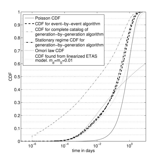
Figure 1: CDFs of inter-event times for synthetic catalogs generated for $b=1$, $c=10^{-3}$, $\alpha=0.7$, $\theta=0.1$, $n=0.7$ ($K=0.21$) and $m_{d}-m_{0}=0.01$. The CDFs of inter-event times are shown for the two algorithms (first event-by-event III.3 and second generation-by-generation III.2) and for the Poisson flow of the background events, the bare Omori law (8) and the theoretical prediction obtained from the linearized equation of the ETAS model developed in SaichevSor06 ; Saichevsor07 .

We have implemented the two algorithms just discussed in the previous subsection and have constructed the corresponding CDFs from the obtained time series for $b=1$, $c=10^{-3}$, $\alpha=0.7$, $\theta=0.1$, $n=0.7$ ($K=0.21$) and $m_{d}-m_{0}=0.01$. Figure 1 shows that both algorithms lead to CDFs which are very close to each other, when the transient regimes of the catalogs generated by the first generation-by-generation algorithm are removed. Using the whole catalog including the transient part for the first algorithm leads to very large distortions. We interpret the remaining slight difference between the CDFs of inter-event times for the first and second algorithms after removal of the transient as due to the residual influence of the transient part of the catalog in the first generation-by-generation algorithm III.2. Figure 1 also shows for comparison the inter-event CDFs of (i) the Poisson flow of the background events, (ii) the bare Omori law (8) and (iii) the theoretical prediction obtained from the linearized equation of the ETAS model developed in SaichevSor06 ; Saichevsor07 confirming the need to go to the nonlinear description SorSaiUtk08 .

IV Results and performance of stochastic declustering methods (SDM and MISD)

IV.1 Previous tests of Zhuang et al. ZhuangOgata04 ; Zhuangetal02 ; OgaZhu06

As mentioned before, Zhuang et al. ZhuangOgata04 ; Zhuangetal02 ; OgaZhu06 applied their declustering procedure described in section II.1 to real earthquake catalogs over four geographical regions: New Zealand (NZ), Central and Western Japan (CJ and WJ) and Northern China (NC). Table 1 provides the results of their SDM applied to these four regions.

Our main remark is that no error or uncertainty analysis is reported and no study of the impact of the lower magnitude threshold used in the catalog is performed. This is particularly worrisome, given the demonstration that parameter estimations are significantly biased when the minimal observable (registerable) magnitude $m_{d}$ is different from (usually larger than) the minimal event magnitude $m_{0}$ able to produce aftershocks Sorwerner ; SaiSor06 .

In a later paper, Zhuang et al. Zhuangetal08 reported some synthetic tests to assess the reliability of the SDM in the ideal case where $m_{d}=m_{0}$. They quoted “good reconstruction results”. However, the parameters estimated with their SDM ($c\approx 0.0004,\;\alpha\approx 0.57,\;\theta\approx 0.014,\;n\approx 0.25$) were very different from the true parameters ($c=0.0002,\;\alpha\approx 0.65,\;\theta=0.12,\;n\approx 0.99$) used to generate the synthetic catalogs. Very worrisome is the very large error in the value of the branching ratio $n$. The true value $n=0.99$ corresponds to a system close to critical branching in which triggering of multiple generations is expected to be very strong since $99\%$ of events are triggered on average while only $1\%$ are exogenous HStrigger03 . In contrast, the estimated value $n\approx 0.25$ would be interpreted as a relatively weak triggering regime in which three-quarters of the events are exogenous.

IV.2 Previous tests of Marsan and Lengliné Marsan07

Unlike the SDM of Zhuang et al, the MISD method was partially verified. Marsan and Lengliné generated synthetic catalogs with the parameters $b=1$, $c=0.01$, $\alpha=0.87$, $\theta=0.2$, $n=0.9$ and $\mu=0.25$. Applying the MISD to that catalog, Marsan and Lengliné could estimate the background rate $\mu^{est}=0.248\pm 0.01$, very close to the true value. The estimates of the other parameters were reported to be also good Marsan07 .

IV.3 Self-consistency of parameter estimations of $n$ and $\alpha$ from synthetic catalogs

IV.3.1 A modifications to SDM (henceforth referred to as mSDM)

In the above presentation, we have considered only the thinning probabilities of events in a catalog. But Zhuang et al’s method contains in addition a determination of the conditional intensity function (12) obtained by using an iterative search procedure with the maximum likelihood $L(\Theta)$ Daley_VJ . Specifically, the search procedure determines the set of parameters $\Theta$ of the model for which the thinning probabilities are best consistent with the conditional intensity $\lambda(t,M|H_{t_{k}})$. Zhuang et al. used the first order algorithm of Davidson-Fletcher-Powell to find the sought maximum of the likelihood function. This method suffers from the need to calculate the derivatives of $\lambda(t,M|H_{t_{k}})$ and $L(\Theta)$, which makes errors accumulate and slows down the calculations.

In the present work, we use the Nelder-Mead simplex method which is significantly more efficient than the first-order Davidson-Fletcher-Powell algorithm. In addition, we recalculate the probabilities $\rho_{ij}$ for each estimation of the likelihood function rather than at each iteration as performed in the SDM version used by Zhuang et al. Our approach increases the computation time of a single iteration but actually provides a significant gain as the number of iterations needed for convergence is greatly reduced.

The set of parameters $\Theta^{d}$ obtained from the maximization of the likelihood function corresponds to the direct estimation. The priority is to verify whether the direct estimation is good enough. Then, we need to check that the catalog reconstructed using thinning probabilities also provides good estimates of the model parameters.

IV.3.2 Applying the modified SDM (mSDM) to two-dimensional data

To check the goodness of the direct estimation by the mSDM, we generated 5 catalogs of 2500 events for different values of $\alpha$ and $n$ and fixed $c=0.001$, $b=1$ and $\theta=0.5$. As one can see from the results presented in table 2, the direct estimation can be quite far off, in particular for the parameters $\theta$ and $n$. But the errors turn out to be smaller than with the thinning probabilities that will be presented below. One of the origins for the errors is the limited length of the synthetic catalog, nothwithstanding the use of an intensionally large value of $\theta=1/2$ leading to a rather short memory (compared to that for smaller values of $\theta$ used below). The SDM and mSDM need more events to reduce the errors in the parameter estimation. Further below, we will consider the relationship between the length of a catalog that is needed to obtain reasonable results and the memory quantified by the exponent $\theta$).

IV.3.3 Targeted parameters

As a first test, we assume known the parameters of the ETAS process generating the synthetic catalogs. For instance, we can assume that the use of the mSDM led us to the true values of parameters $\Theta^{d}\approx\Theta^{s}$. We then apply the SDM and the MISD to determine the background and triggered events. From this knowledge, we can estimate directly the branching ratio $n$ and the fertility exponent $\alpha$ and compare them with the true values. We stress that we use the exact parameters that enter in the generation of the synthetic catalogs to find the thinning probabilities (2) to perform this test. Thus, any discrepancy between the estimation of $n$ and $\alpha$ using the thinning probabilities should be attributed only to errors in the reconstruction of the tree of ancestry through the thinning probabilities.

The first key parameter of interest is the branching ratio, which can be estimated from the knowledge of the number of exogenous events within the data set, according to

$$n_{e}=1-\frac{{\rm number\;of\;background\;events}}{\rm total\;number\;of\;events}~{},$$ (19)

where the subscript e indicates that $n_{e}$ is experimental or estimated value.

Knowing the tree structure of events obtained from the declustering method, we can estimate directly the productivity law (9). Specifically, the tree structure allows us to calculate straightforwardly the mean number of direct aftershocks triggered by a given event, and then to test how this mean number depends on the magnitude of the mother event. Given the true law (9), the estimated dependence of the number of aftershocks as a function of the magnitude of the main shock is fitted by the following expression

$$\hat{Q}(M)=K^{*}\cdot 10^{A^{*}\cdot M}~{},$$ (20)

where $(K^{*},A^{*})$ are determined using standard optimization algorithms. The estimated values can then be compared to the true values $(K,\alpha)$ used to generate the synthetic catalogs.

To account for the fact that, in real time series, small events below a magnitude detection threshold $m_{d}>m_{0}$ are not detected, we also investigate the influence of this detection threshold on the estimated parameters. Intuitively, as demonstrated in Refs. Sorwerner ; SaiSor06 , missing events lead to misinterpret triggered events as exogenous background events, since the chain of causal triggering may be ruptured. This may influence severely the estimation of the background rate and therefore of the parameters controlling the fertility and triggering efficiency of past events. A good diagnostic of the effect of missed events is the branching ratio $n$ Sorwerner ; SaiSor06 . We thus evaluate the apparent branching ratio estimated by the declustering method on the catalog of events with magnitudes larger than $m_{d}$ according to the following formula

$$n_{t}=\frac{\rm number\;of\;aftershocks\;with\;M>m_{d},\;whose\;mother\;also\;has\;M>m_{d}}{\rm number\;of\;all\;events\;with\;M>m_{d}}$$ (21)

We also will test how the truncation affects the estimated parameters, and does this correspond to the theoretical dependance SaichevSor06 ; Saichevsor07 .

IV.3.4 First test on declustering Poisson sequences

We first applied the SDM and MISD to catalogs generated by a simple Poisson process, obtained from the formulation of section III.1 by imposing the value $K=0$ in (9). As a consequence, only exogenous background events without any triggered event are generated in synthetic catalogs with intensity imposed equal to $\mu=1$. A correct declustering algorithm should find $n=0$ and a background rate ${\hat{\mu}}=1$.

Applying the SDM on tens of catalogs each containing between 1000 and 2000 events with magnitudes $M>0$, we recovered the correct result that the branching ratio is $n=0$ in every case (all probabilities $\phi_{j}$ are found exactly equal to 1) and the background rate is estimated as ${\hat{\mu}}=1\pm 0.05$, close and consistent with the true value.

On a technical note, the arrest criterion controlling the convergence of the algorithm was found to play a strong role, much more significant for time-domain-only catalogs than when the catalogs include spatial information. We found these good results only for an arrest criterion corresponding to differences smaller than $0.0001$ between the parameter values of successive iterations. We kept this value for all subsequent tests, as a compromise between accuracy of the convergence and numerical feasibility.

On the same catalogs, the MISD method found however nonzero probabilities $\rho_{ij}$ for $i\neq j$ and, as a result, a nonzero and actually quite large branching ratio $n=0.23\pm 0.03$. The estimation of the background rate was also not very good ${\hat{\mu}}_{0}=0.81\pm 0.02$ instead of the true value $1$. This means that the MISD method applied in the temporal domain to already declustered catalogs (pure Poisson) misclassifies about $23\%$ of the events as being triggered, while they are all exogenous.

IV.3.5 Tests using catalogs generated by the generation-by-generation algorithm III.2

Test of the SDM. We tested the SDM using data sets generated with various values of $\alpha=0\;-\;0.9$ of the productivity law (9). We generated 10 catalogs of length of $\approx 50,000$ days for each parameters set, with a background rate $\mu_{0}=1$ per day. The duration of the catalogs in terms of days is just to offer a convenient interpretation, as the intrinsic time scale is more generally determined by $1/\mu_{0}$. Each catalog contained about $70,000\;-\;100,000$ events. We removed the first $2000$ events in the first part of the catalogs, roughly corresponding to the first 1500 days, and applied the SDM procedure 20 times to each catalog. Table 3 compiles the obtained values $n_{e}$, $A^{*}$ and $K^{*}$ defined in (19) and (20), reports their standard deviations and compares with the true values $n,\alpha$ and $K$.

We found that the distributions of background rates for the different values of $\alpha=0\;-\;0.9$ are reasonably estimated, with an error of no more than $10\%$. While the estimated branching ratio $n_{e}$ is also reasonably close to the true value for $\alpha$ up to $0.6$ and then starts to systematically deviate for larger $\alpha$’s, the estimated parameters $K^{*}$ and $A^{*}$ are found very far from the true values. In particular, the values of the estimated fertility exponent $A^{*}$ would imply that events of all magnitudes have on average no more than one aftershock, which is very far from being the case, especially for large values of $\alpha$. One partial cause for this bad result is the Omori law which, as shown in fig.1, implies very long inter-event times between direct aftershocks. Some of those intervals can be longer than our catalog and the real productivity will be thus underestimated. Another possible partial cause is that the removal of an initial part of the catalogs to analyze the more stationary regime at later times deletes by construction many events that are mothers of the observed events. This also leads to an underestimation of the triggering productivity. These two explanations suggest that the problem is intrinsic to the application of the SDM to the ETAS model and we do not envision easy fixes.

Test of the MISD method. We applied the MISD method to the same catalogs. Table 4 shows a slight systematic overestimation of the branching ratio $n_{e}$ over the true value $n$. The estimations of $\alpha$ and $K$ are also bad with large systematic errors. The trend of variation of $K$ as a function of $\alpha$ for the fixed true $n=0.26$ is qualitatively reproduced by the dependence of $K^{*}$ as a function of $\alpha$.

We must also report a surprising difference between the SDM and the MISD method. While the standard deviations of the estimated parameters over 10 different synthetic catalogs are sometimes significantly larger for the MISD method compared with the SDM, the former method exhibited sometimes very accurate results for a few catalogs for some specific values of the parameters. For instance, for one of the synthetic catalog generated with the parameters $n=0.26$, $\alpha=0.9$, $K=0.026$ and $\mu_{0}=1$, the MISD method gave the following estimates: $n_{e}=0.255\pm 0.007$, $A^{*}=0.916\pm 0.037$, $K^{*}=0.018\pm 0.007$ and background rate ${\hat{\mu}}_{0}=0.890\pm 0.218$. The existence of such an excellent inversion has to be tampered by the fact that the estimates obtained with the MISD method applied to the other 9 catalogs generated with the same parameters were bad. This suggests a very strong dependence of the performance of the MISD method on the specific stochastic realizations.

Impact of catalog incompleteness. We now report some results on the estimation of parameters by the two declustering methods applied to incomplete catalogs, motivated by the nature of real-life catalogs. The incompleteness is measured by the magnitude threshold $m_{d}>m_{0}$, below which events are missing from the catalogs used for the SDM and MISD method.

First, we focus on the results Sorwerner ; SaiSor06 that the branching ratio $n$ is renormalized into an effective value $n_{t}$ which is a decreasing function of $m_{d}$:

$$n_{t}(m_{d})=\frac{1}{1+\frac{1-n}{n}[10^{\alpha m_{d}}]^{{b\over\alpha}-1}}~{}.$$ (22)

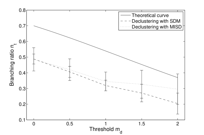
Figure 2: Dependance of the effective branching ratio $n_{t}$ as a function of the threshold magnitude $m_{d}$ of catalog incompleteness. The parameters used to generate the synthetic catalogs with the ETAS model are $b=1,\;c=0.001,\;\theta=0.1,\;n=0.7,\;\alpha=0.7,\;K=0.21$. The dashed (respectively dotted) line correspond to $n_{t}$ obtained by using SDM algorithm (respectively MISD algorithm). The continuous curve is the validated theoretical formula (22).

This prediction was verified by direct simulations with the ETAS model. Here, we test how the incompleteness of catalogs may interfere with the stochastic declustering methods. We generated 50 catalogs with the following set of parameters: $b=1,\;c=0.001,\;\theta=0.1,\;n=0.7,\;\alpha=0.7,\;K=0.21$ and varied $m_{d}$ from $0$ to $2$. Applying the SDM 20 times to each of the 50 synthetic data sets, figure 2 shows that (i) the general trend of decreasing $n_{t}(m_{d})$ as a function of $m_{d}$ is recovered, but (ii) there is a very significant downward bias of approximately $0.2$ over the whole range $0\leq m_{d}\leq 2$. Table 5 shows unsurprisingly that the estimated parameters $A^{*}$ and $K^{*}$ are very far from the true values $\alpha$ and $K$. Using incomplete catalogs cannot be expected to improve the estimation of parameters which is already bad for complete catalogs. For smaller values of the true branching ratio $n$, the discrepancy is smaller between the reconstructed $n_{t}$ and the theoretical formula (22). For instance, for $n=0.4$, the difference between the estimated $n_{t}$ and the formula (22) decreases from $0.1$ for $m_{d}=0$ (no incompleteness) to almost zero for $m_{d}=2$ for which $n_{t}(m_{d}=2)\approx 0.04$.

Typical results for the MISD method are reported in table 6 for the set of true parameters $n=0.7,\alpha=0.7$ and $K=0.21$, for $m_{d}$ varying from $0$ to $2$. While the estimated $n_{e}$ for $m_{d}=0$ (no incompleteness) are as good as with the direct SDM estimation method, the other estimated parameters are strongly biased. For incomplete catalogs $m_{d}>0$, we observe a large over-estimation of $n_{t}$ and significant errors in the other estimated parameters.

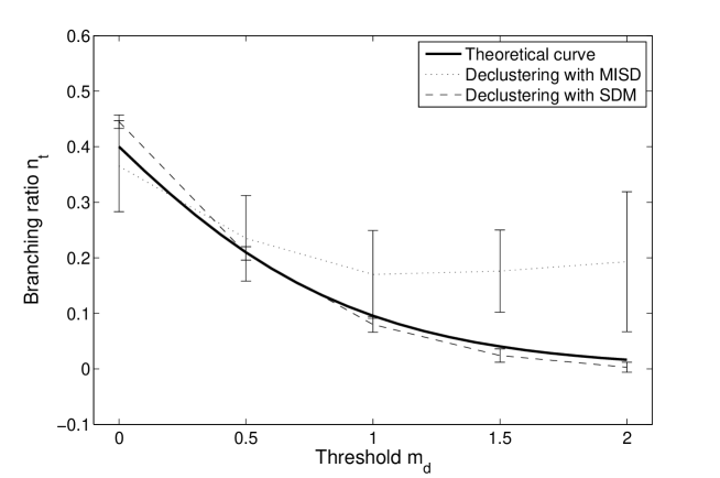
Figure 3: Dependance of the effective branching ratio $n_{t}$ as a function of the threshold magnitude $m_{d}$ of catalog incompleteness. The parameters used to generate the synthetic catalogs with the ETAS model are $b=1,\;c=0.001,\;\theta=0.1,\;n=0.4,\;\alpha=0.2,\;K=0.32$. The dashed (respectively dotted) line correspond to $n_{t}$ obtained by using the SDM algorithm (respectively the MISD algorithm). The continuous curve is the validated theoretical formula (22).

Another test is provided by comparing the CDFs of background events in the incomplete catalogs as a function of $m_{d}$ obtained by the declustering methods with the true CDFs. We found that, the larger is the true branching ratio $n$, the larger is the discrepancy between the true and reconstructed CDFs of background events, using both declustering methods for all $m_{d}$ values. For $n\leq 0.4$, the reconstructed background CDFs are in reasonable agreement with the theoretical formula (22) with typical errors of about $10\%$ (See tables 9 and 5 and figure 3). For large branching ratios, the errors are too large and the declustering methods are unreliable.

Comparing figures 2 and 3, one can notice that MISD becomes less precise for large thresholds $m_{d}$. That is more likely caused by the smaller lengths of the catalogs.

IV.3.6 Tests using catalogs generated by the event-by-event algorithm III.3

The same tests as reported in the previous subsection were performed on catalogs generated by the event-by-event algorithm III.3. We recall that our motivation for using this alternative algorithm is to test for the expected influence of transient regimes, which are absent by construction in the synthetic catalogs obtained with the event-by-event algorithm III.3.

Using one hundred catalogs of 2000 events (10 for each $\alpha$ going from $0$ to $0.9$) generated with algorithm III.3, we applied the SDM and obtained the results summarized in table 7. The results are similar to those of table 3, with a reasonable estimation $n_{e}$ but estimated $A^{*}$ and $K^{*}$ very far from the true values $\alpha$ and $K$.

Ten catalogs of 4000 events were generated with the parameters $b=1,c=0.001,\theta=0.1,n=0.6,\alpha=0.2$ and $K=0.48$. Incompleteness was introduced at magnitude thresholds $m_{d}$ varying from $0$ to $2$, reducing the size of catalogs to the $m_{d}$-dependent number $\approx N_{m_{d}}$ events. Applying the SDM to these incomplete catalogs, we obtained the results shown in table 8. As mentioned above, the estimated $n_{e}$ is found in better agreement with the theoretical prediction (22) for the largest $m_{d}$ values for which $n_{t}$ is the smallest.

Table 9 shows that the MISD method gives results similar to those previously obtained in table 6. The estimated value of background rate is ${\hat{\mu}}_{0}=0.165\pm 0.198$, which is quite different from the true value $1$.

V Tests on the influence of memory (exponent $\theta$), background rate and catalog lengths

V.1 Influence of the value of the memory exponent $\theta$

We now test one possible origin for the rather bad performance of the SDM and MISD method when using the thinning probabilities, namely the very long memory quantified by the small value of the exponent $\theta$ (as defined in expression (8)) used in the simulations.

A series of tests were made with a larger value of $\theta=0.5$, corresponding to significantly shorter memory. We varied the values of $n$ and $\alpha$, while fixing the other parameters $c=0.001$, $b=1$, $\mu=1$. We generated 10 catalogs of 2500 events each using the event-by-event algorithm described in subsection III.3 for each set of parameters. We implemented both declustering algorithms 20 times to each catalog. Table 10 presents the resulting estimates of the parameters. The most striking result is that the branching ratio $n$ estimated by the SDM is in general very good. While the MISD method is not reliable for estimated the branching ratio $n$, it is better for the estimation of the productivity exponent $\alpha$, especially for large values. The results presented in table 10, when put in comparison with those of the previous tables obtained with much smaller values of the memory exponent $\theta$, illustrates clearly the impact of the long-memory on the declustering results.

V.2 Case of a single large main shock triggering aftershocks

In another series of tests, we check if the SDM or MISD are able to determine a pure tree branching process emanating from a single source. In this goal, we removed all spontaneous events except one, the first “main shock”. This corresponds to imposing $\mu=0$. In order to have sufficiently many events in the catalogs, we take the magnitude of the single main shock large ($M_{1}=7$) and also impose large values for the parameters $n$ and $\alpha$ to produce long sequences of events. The parameter $\theta$ was taken equal to 0.1 (long memory). We found that the SDM recognized the existence of the only background event in two tests out of three (for $\alpha=0.8$). In contrast, the MISD lacks efficiency in such conditions and proposes significantly non-zero values for the background rate $\mu$. The estimation of $n$ with formula (19) cannot provide good results because it should give $n_{e}\to 1$ (only one background event) for large catalogs. Other methods of estimating the branching ratio described in HStrigger03 gave even worse results, with $n_{e}>1$.

V.3 Influence of catalog lengths

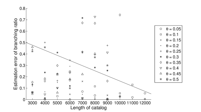
Figure 4: Error of the direct estimation of the branching ratio by the mSDM as a function of catalog length for different values of $\theta$.

As mentioned above, two effects combine to limit the efficiency of the SDM and MISD methods: the smallness of the exponent $\theta$ leading to very long memory and the limited length of the catalogs. We investigated how these two effects are inter-related in practice. Using algorithm III.2, we generated 100 catalogs with variable numbers of events (from $3000$ to $12000$) and for various values of $\theta$ (from $0.05$ up to $0.5$). The other parameters were fixed at $b=1$, $\alpha=0.7$, $c=0.001$, $n=0.7$. We then applied the mSDM to each catalog. Fig.4 shows the estimation error of the branching ratio $n$. One can observe very large variations from realization to realization and a weak tendency for estimation errors to decrease with the length of the catalogs.

To be more quantitative, let us introduce the cumulative error ratio defined as the sum of squares of relative errors over all parameters:

$$\varepsilon=\sum\limits_{i=1}^{5}\left(1-\frac{\Theta_{i}^{d}}{\Theta_{i}^{s}}\right)^{2},\quad(\Theta_{1-5}=b,\alpha,c,\theta,n).$$ (23)

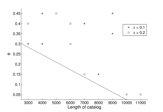
Figure 5: Dependence of $\varepsilon$ as a function of catalog lengths is shown for two classes of catalogs sorted according to their estimation errors as defined by equation (23).

The dependence of $\varepsilon$ as a function of catalog lengths is shown in fig.5 for a number of realizations. Again, one can observe an overall decrease of the estimation error with the length of the catalogs, decorated by a very large variability from catalog to catalog.

As an illustration of the quality of the reconstruction of the tree structure of ancestry in different catalogs, we took 7 catalogs with $\varepsilon<0.1$ (best results) and several catalogs with $\varepsilon>1$ (bad results) and determined the percentage of background events recognized as background and of aftershocks recognized as aftershocks. For catalogs with the best directly estimated parameters, the percentage were 66% and 72% respectively, while for the “bad” catalogs the results were 9% and 93% (i.e., almost all events were incorrectly recognized as aftershocks).

VI Conclusions

Many time series in natural and social sciences can be seen as embodying an interplay between exogenous influences and an endogenous organization. We have used a simple model of events occurring sequentially, in which future events are influenced (partially triggered) by past events to ask the question of how well can one disentangle the exogenous events from the endogenous ones.

The exogenous events are modeled here by a Poisson flow of so-called background events with constant intensity $\mu_{0}$. The ETAS specification of the conditional self-excited Hawked Poisson model has been used. It contains three principal ingredients: (i) a long Omori-like power law memory of the influence of past events on future events, (ii) a Gutenberg-Richter-like distribution of event magnitudes and (iii) a fertility law expressing how many events are triggered by a given event as a function of its magnitude.

In order to separate background events from triggered events, we have implemented and compared two so-called “declustering” algorithms, the SDM introduced by Zhuang et al. Zhuangetal02 ; Zhuangthesis and the MISD method proposed by Marsan and Lengliné Marsan07 . We have applied these two methods to synthetic catalogs generated by two algorithms using the ETAS model, the generation-by-generation algorithm III.2 and the event-by-event algorithm III.3.

We specifically address the problem of reconstructing the tree of ancestry of the sequence of events in recorded catalogs. In particular, one main goal is to distinguish the exogenous shocks (background events) from the endogenous (triggered events). For these problems, we find that declustered catalogs obtained from synthetic catalogs generated with the ETAS model are rather unreliable, when using catalogs with of the order of thousands of events, typical of realistic applications. The estimated rates of exogenous events suffer from large errors. The key branching ratio $n$, quantifying the fraction of events that have been triggered by previous events, is also badly estimated in general with these approaches. We find however that the errors tend to be smaller and perhaps acceptable in some cases for the smaller fertility exponent $\alpha<0.6$ and for the smaller branching ratio $n<0.4$ typically. Results become better when the memory exponent $\theta$ is increased, i.e., when the memory is shortened. We do not find significantly better performance of the SDM versus the MISD method or vice-versa, with the curious observation that the MISD method is sometimes very precise for some catalog realizations, but this property is not robust with respect to other stochastic realizations. We have also investigated the role of incompleteness on declustering, and found that this is not the essential limiting problem.

We should however make clear that these rather negative results are not necessarily opposed to the more positive results reported by Zhuang et al. and Marsan and Lengliné, which refer to a different problem, that of the direct estimation of the model parameters (and not of the tree of ancestry and of the distinction between exogenous and endogenous events). Our larger ambition to reconstruct the tree of ancestry has identified clearly intrinsic limits of the inversion process.

It appears that the high level of randomness together with the very long memory makes the stochastic reconstruction of trees of ancestry and the estimation of the key parameters quite unreliable. Technically, we find the coexistence of many coexisting stochastic reconstructions with different parameter estimates, and it is not obvious how to select what should be the right one. This question is reminiscent of complex optimization problem in the presence of a very large number of almost equivalent solutions, as occurs in so-called NP-complete problems. There thus appears to be fundamental limitations intrinsic to this class of models.

Acknowledgements: We are grateful to David Marsan for discussions and help in using his MISD algorithm as well as feedbacks on the testing procedure. We thank Anne-Marie Christophersen, David Marsan Guy Ouillon, Max Werner and Jiancang Zhuang for useful feedbacks on an earlier version of the manuscript.

Table 1: Estimated parameters of the ETAS model obtained by the stochastic declustering method (SDM) of Zhuang et al. ZhuangOgata04 ; Zhuangetal02 ; OgaZhu06 described in section II.1 applied to real earthquake data from New Zealand (NZ), Central and Western Japan (CJ and WJ) and Northern China (NC). The quoted values for the fertility exponent $\alpha$ differ from those reported by Zhuang et al. by the conversion factor $\ln 10$ accounting for our use of base-ten logarithm and exponential compared with the natural logarithm and exponential used by Zhuang et al.

Region	$c$	$\theta$	$\alpha$	$K$	$n$
NZ	0.017	0.164	0.389	0.335	0.548
CJ, WJ	0.040	0.250	0.495	0.204	0.404
NC	0.003	0.030	0.499	0.546	1.090

Table 2: Direct estimation of the parameters $\Theta^{s}$ with the modified SDM compared with the true parameters $\Theta^{d}$ of the ETAS model used to generate the synthetic catalogs by the event-by-event algorithm.

#		$b$	$\alpha$	$c$	$\theta$	$n$
1	$\Theta^{s}$	1.00	0.20	0.00100	0.50	0.20
	$\Theta^{d}$	3.80	0.27	0.00103	0.54	0.07
2	$\Theta^{s}$	1.00	0.50	0.00100	0.50	0.50
	$\Theta^{d}$	0.44	0.30	0.00050	0.21	0.78
3	$\Theta^{s}$	1.00	0.80	0.00100	0.50	0.80
	$\Theta^{d}$	1.00	0.96	0.00160	0.64	0.96
4	$\Theta^{s}$	1.00	0.20	0.00100	0.50	0.80
	$\Theta^{d}$	0.33	0.24	0.00240	0.84	0.92
5	$\Theta^{s}$	1.00	0.80	0.00100	0.50	0.20
	$\Theta^{d}$	1.00	0.76	0.00070	0.41	0.10

Table 3: Estimated parameters $n_{e}$, $A^{*}$ and $K^{*}$ with the SDM compared with the true parameters $n=0.26$, $\alpha$ and $K$ of the ETAS model used to generate the synthetic catalogs by the generation-by-generation algorithm. The other parameters have been fixed to $m_{d}=m_{0}=0$, $b=1$, $c=0.002$, and $\theta=0.19$.

#	$n$	$n_{e}$	$\alpha$	$A^{*}$	$K$	$K^{*}$
1	0.26	$0.237\pm 0.009$	0.0	$0.024\pm 0.041$	0.260	$0.930\pm 0.097$
2	0.26	$0.239\pm 0.010$	0.1	$0.015\pm 0.060$	0.234	$0.939\pm 0.118$
3	0.26	$0.240\pm 0.010$	0.2	$-0.005\pm 0.041$	0.208	$0.960\pm 0.087$
4	0.26	$0.237\pm 0.009$	0.3	$-0.048\pm 0.039$	0.182	$1.034\pm 0.079$
5	0.26	$0.240\pm 0.012$	0.4	$-0.059\pm 0.061$	0.156	$1.030\pm 0.134$
6	0.26	$0.240\pm 0.018$	0.5	$-0.092\pm 0.053$	0.130	$1.065\pm 0.115$
7	0.26	$0.226\pm 0.012$	0.6	$-0.104\pm 0.073$	0.104	$1.082\pm 0.142$
8	0.26	$0.225\pm 0.022$	0.7	$-0.084\pm 0.150$	0.078	$1.043\pm 0.208$
9	0.26	$0.207\pm 0.029$	0.8	$0.004\pm 0.453$	0.052	$0.989\pm 0.370$
10	0.26	$0.143\pm 0.028$	0.9	$-0.151\pm 0.043$	0.026	$1.097\pm 0.068$

Table 4: Estimated parameters $n_{e}$, $A^{*}$ and $K^{*}$ with the MISD compared with the true parameters $n=0.26$, $\alpha$ and $K$ of the ETAS model used to generate the synthetic catalogs by the generation-by-generation algorithm. The other parameters have been fixed to $m_{d}=m_{0}=0$, $b=1$, $c=0.002$, and $\theta=0.19$.

#	$n$	$n_{e}$	$\alpha$	$A^{*}$	$K$	$K^{*}$
1	0.26	$0.319\pm 0.048$	0.0	$0.332\pm 0.265$	0.260	$0.931\pm 0.450$
2	0.26	$0.299\pm 0.035$	0.1	$0.465\pm 0.535$	0.234	$1.077\pm 1.106$
3	0.26	$0.328\pm 0.064$	0.2	$0.352\pm 0.264$	0.208	$0.925\pm 0.693$
4	0.26	$0.343\pm 0.061$	0.3	$0.488\pm 0.373$	0.182	$0.847\pm 1.047$
5	0.26	$0.336\pm 0.062$	0.4	$0.355\pm 0.134$	0.156	$0.955\pm 0.678$
6	0.26	$0.332\pm 0.069$	0.5	$0.579\pm 0.265$	0.130	$0.373\pm 0.372$
7	0.26	$0.322\pm 0.060$	0.6	$1.011\pm 0.912$	0.104	$0.293\pm 0.325$
8	0.26	$0.320\pm 0.113$	0.7	$0.815\pm 0.488$	0.078	$0.295\pm 0.312$
9	0.26	$0.337\pm 0.151$	0.8	$0.818\pm 0.223$	0.052	$0.122\pm 0.128$
10	0.26	$0.320\pm 0.174$	0.9	$0.900\pm 0.449$	0.026	$0.126\pm 0.143$

Table 5: Estimated parameters $n_{e}$, $A^{*}$ and $K^{*}$ with the SDM compared with the true parameters $n=0.7$, $\alpha=0.7$ and $K=0.21$ of the ETAS model used to generate the synthetic catalogs by the generation-by-generation algorithm, for various magnitude threshold $m_{d}$ of incompleteness. The other parameters have been fixed to $b=1$, $c=0.001$, and $\theta=0.1$. $N_{m_{d}}$ is the number of events in the incomplete catalogs.

#	$m_{d}$	$N_{m_{d}}$	$n_{e}$	$A^{*}$	$K^{*}$
1	0.0	2000	$0.488\pm 0.032$	$-0.045\pm 0.400$	$1.037\pm 0.214$
2	0.5	2000	$0.406\pm 0.035$	$0.135\pm 0.784$	$1.085\pm 0.437$
3	1.0	1000	$0.319\pm 0.034$	$-0.006\pm 0.286$	$1.201\pm 0.491$
4	1.5	500	$0.271\pm 0.056$	$-0.054\pm 0.116$	$1.376\pm 0.574$
5	2.0	150	$0.204\pm 0.067$	$-0.047\pm 0.094$	$1.495\pm 0.769$

Table 6: Estimated parameters $n_{e}$, $A^{*}$ and $K^{*}$ with the MISD method compared with the true parameters $n=0.7$, $\alpha=0.7$ and $K=0.21$ of the ETAS model used to generate the synthetic catalogs by the generation-by-generation algorithm, for various magnitude threshold $m_{d}$ of incompleteness. The other parameters have been fixed to $b=1$, $c=0.001$, and $\theta=0.1$. $N_{m_{d}}$ is the number of events in the incomplete catalogs.

#	$m_{d}$	$N_{m_{d}}$	$n_{e}$	$A^{*}$	$K^{*}$
1	0.0	4000	$0.486\pm 0.074$	$0.930\pm 0.448$	$0.167\pm 0.166$
2	0.5	1300	$0.420\pm 0.069$	$0.873\pm 0.878$	$0.089\pm 0.188$
3	1.0	400	$0.345\pm 0.060$	$-0.357\pm 2.804$	$0.239\pm 0.497$
4	1.5	130	$0.327\pm 0.089$	$0.249\pm 1.521$	$0.168\pm 0.686$
5	2.0	40	$0.296\pm 0.097$	$-0.771\pm 3.214$	$0.002\pm 0.874$

Table 7: Estimated parameters $n_{e}$, $A^{*}$ and $K^{*}$ with the SDM compared with the true parameters $n=0.26$, $\alpha$ and $K$ of the ETAS model used to generate the synthetic catalogs using the event-by-event algorithm. The other parameters are fixed to $m_{d}=0$, $b=1$, $c=0.002$, and $\theta=0.19$.

#	$n$	$n_{e}$	$\alpha$	$A^{*}$	$K$	$K^{*}$
1	0.26	$0.244\pm 0.024$	0.0	$0.042\pm 0.092$	0.260	$0.845\pm 0.211$
2	0.26	$0.238\pm 0.027$	0.1	$0.033\pm 0.082$	0.234	$0.856\pm 0.203$
3	0.26	$0.248\pm 0.022$	0.2	$0.016\pm 0.077$	0.208	$0.895\pm 0.176$
4	0.26	$0.246\pm 0.036$	0.3	$-0.014\pm 0.075$	0.182	$0.940\pm 0.173$
5	0.26	$0.233\pm 0.011$	0.4	$-0.032\pm 0.070$	0.156	$0.967\pm 0.137$
6	0.26	$0.234\pm 0.024$	0.5	$-0.025\pm 0.072$	0.130	$0.960\pm 0.152$
7	0.26	$0.233\pm 0.017$	0.6	$-0.101\pm 0.065$	0.052	$1.069\pm 0.107$
8	0.26	$0.216\pm 0.024$	0.7	$-0.074\pm 0.060$	0.104	$1.011\pm 0.116$
9	0.26	$0.206\pm 0.021$	0.8	$0.179\pm 0.952$	0.078	$1.005\pm 0.314$
10	0.26	$0.216\pm 0.210$	0.9	$-0.121\pm 0.055$	0.026	$1.151\pm 0.205$

Table 8: Estimated parameters $n_{e}$, $A^{*}$ and $K^{*}$ with the SDM compared with the true parameters $n=0.6$, $\alpha=0.2$ and $K=0.48$ of the ETAS model used to generate the synthetic catalogs by the event-by-event algorithm, for various magnitude threshold $m_{d}$ of incompleteness. The other parameters have been fixed to $b=1$, $c=0.001$, and $\theta=0.1$.

#	$m_{d}$	$N_{m_{d}}$	$n_{e}$	$A^{*}$	$K^{*}$
1	0.0	4000	$0.445\pm 0.012$	$-0.004\pm 0.048$	$0.960\pm 0.115$
2	0.5	1300	$0.208\pm 0.012$	$0.000\pm 0.0345$	$0.968\pm 0.098$
3	1.0	400	$0.080\pm 0.014$	$-0.004\pm 0.022$	$1.013\pm 0.085$
4	1.5	130	$0.024\pm 0.012$	$0.003\pm 0.017$	$0.977\pm 0.073$
5	2.0	40	$0.003\pm 0.009$	$0.009\pm 0.018$	$0.932\pm 0.077$

Table 9: Estimated parameters $n_{e}$, $A^{*}$ and $K^{*}$ with the MISD method compared with the true parameters $n=0.4$, $\alpha=0.2$ and $K=0.32$ of the ETAS model used to generate the synthetic catalogs by the generation-by-generation algorithm, for various magnitude threshold $m_{d}$ of incompleteness. The other parameters have been fixed to $b=1$, $c=0.001$, and $\theta=0.1$.

#	$m_{d}$	$N_{m_{d}}$	$n_{e}$	$A^{*}$	$K^{*}$
1	0.0	2000	$0.365\pm 0.082$	$0.380\pm 0.198$	$0.618\pm 0.393$
2	0.5	2000	$0.235\pm 0.079$	$0.275\pm 1.462$	$0.324\pm 0.450$
3	1.0	1000	$0.170\pm 0.077$	$0.041\pm 2.094$	$0.348\pm 0.597$
4	1.5	500	$0.176\pm 0.074$	$0.065\pm 1.501$	$0.364\pm 0.651$
5	2.0	150	$0.193\pm 0.126$	$0.114\pm 0.991$	$0.411\pm 0.621$

Table 10: Estimated parameters $n_{e}$, $A^{*}$ and $K^{*}$ with the SDM and MISD compared with the true parameters $n$, $\alpha$ and $K$ of the ETAS model used to generate the synthetic catalogs by the event-by-event algorithm. The other parameters have been fixed to $m_{d}=m_{0}=0$, $b=1$, $c=0.001$, and $\theta=0.5$.

#	method	$n$	$\alpha$	$K$	$n_{e}$	$A^{*}$	$K^{*}$
1	SDM	0.2	0.2	0.16	$0.199\pm 0.009$	$-0.020\pm 0.042$	$0.999\pm 0.087$
2	MISD	0.2	0.2	0.16	$0.313\pm 0.019$	$1.116\pm 1.203$	$0.367\pm 0.285$
3	SDM	0.5	0.5	0.25	$0.502\pm 0.020$	$-0.061\pm 0.076$	$1.004\pm 0.156$
4	MISD	0.5	0.5	0.25	$0.546\pm 0.018$	$0.970\pm 0.828$	$0.501\pm 0.363$
5	SDM	0.8	0.8	0.16	$0.698\pm 0.072$	$0.024\pm 0.481$	$0.941\pm 0.250$
6	MISD	0.8	0.8	0.16	$0.755\pm 0.045$	$0.700\pm 0.108$	$0.347\pm 0.209$
7	SDM	0.8	0.2	0.64	$0.793\pm 0.014$	$0.009\pm 0.068$	$0.942\pm 0.141$
8	MISD	0.8	0.2	0.64	$0.804\pm 0.016$	$0.352\pm 0.337$	$0.626\pm 0.272$
9	SDM	0.2	0.8	0.04	$0.168\pm 0.021$	$-0.160\pm 0.081$	$1.187\pm 0.159$
10	MISD	0.2	0.8	0.04	$0.259\pm 0.037$	$0.694\pm 0.128$	$0.175\pm 0.132$

which

References

- (1) Beran, J., Statistics for Long-Memory Processes (Monographs on Statistics and Applied Probability), Chapman & Hall/CRC (1994).
- (2) Brémaud, P., Point Processes and Queues, Springer, New York (1981).
- (3) Brémaud, P. and L. Massoulié, Stability of nonlinear Hawkes processes, Ann. Probab. 24 (3), 1563-1588 (1996).
- (4) Brémaud, P. and L. Massoulié, Hawkes branching point processes without ancestors Journal of Applied Probability 38 (1), 122-135 (2001).
- (5) Crane, R. and D. Sornette, Robust dynamic classes revealed by measuring the response function of a social system, Proc. Nat. Acad. Sci. USA 105 (41), 15649-15653 (2008).
- (6) Daley, D.J. and Vere-Jones, D., An introduction to the theory of point processes, Vol.1: Elementary theory and methods, 2nd ed., Springer (2003).
- (7) Deschatres, F. and D. Sornette, The Dynamics of Book Sales: Endogenous versus Exogenous Shocks in Complex Networks, Phys. Rev. E 72, 016112 (2005).
- (8) Felzer, K.R., T.W. Becker, R.E. Abercrombie, G. Ekström and J.R. Rice, Triggering of the 1999 Mw 7.1 Hector Mine earthquake by aftershocks of the 1992 Mw 7.3 Landers earthquake, J. Geophys. Res., 107, 2190, doi:10.1029/2001JB000911 (2002).
- (9) Hawkes, A. G., Point spectra of some mutually exciting point processes, J. R. Stat. Soc., Ser. B, 33, 438-443 (1971).
- (10) Hawkes, A. G., and L. Adamapoulos, Cluster models for earthquakes: Regional comparisons, Bull. Int. Stat. Inst., 45, 454-461 (1973).
- (11) Hawkes, A. G., and D. Oakes, A cluster representation of a self-exciting process, J. Appl. Probab., 11, 493-503 1974).
- (12) Helmstetter, A. and D. Sornette, Sub-critical and supercritical regimes in epidemic models of earthquake aftershocks, J. Geophys. Res. 107, NO. B10, 2237, doi:10.1029/2001JB001580, (2002).
- (13) Helmstetter, A. and D. Sornette, Importance of direct and indirect triggered seismicity in the ETAS model of seismicity, Geophys. Res. Lett. 30 (11) doi:10.1029/2003GL017670 (2003).
- (14) Helmstetter and D. Sornette, Foreshocks explained by cascades of triggered seismicity, J. Geophys. Res. (Solid Earth) 108 (B10), 2457 10.1029/2003JB002409 01 (2003)
- (15) Helmstetter, A., D. Sornette and J.-R. Grasso, Mainshocks are Aftershocks of Conditional Foreshocks: How do foreshock statistical properties emerge from aftershock laws, J. Geophys. Res., 108 (B10), 2046, doi:10.1029/2002JB001991 (2003).
- (16) Johansen, A. and D. Sornette Endogenous versus Exogenous Crashes in Financial Markets, in press in “Contemporary Issues in International Finance” (Nova Science Publishers, 2004) (http://arXiv.org/abs/cond-mat/0210509)
- (17) Marsan D. and O. Lengliné, Extending Earthquakes’ Reach Through Cascading, Science 319 (5866), 1076-1079 (2008).
- (18) MISD: http://www.lgit.univ-savoie.fr/MISD/misd.html
- (19) Ogata Y., On Lewis’ simulation method for point processes. IEEE Translations on Information Theory, IT-27, 23–31 (1981).
- (20) Ogata, Y., Statistical models for earthquake occurrences and residual analysis for point processes, Journal of the American Statistical Association 83 (401), 9-27 (1988).
- (21) Ogata Y. and Zhuang J., Space time ETAS models and an improved extension Tectonophysics, 413, 13-23 (2006).
- (22) Ouillon, G. and D. Sornette, Magnitude-Dependent Omori Law: Theory and Empirical Study, J. Geophys. Res., 110, B04306, doi:10.1029/2004JB003311 (2005).
- (23) Osorio, I., M.G. Frei, D. Sornette, J. Milton and Y.-C. Lai, Epileptic seizures: quakes of the brain, in press in Phys. Rev. Letts. (http://arxiv.org/abs/0712.3929)
- (24) Ozaki, T., Maximum Likelihood Estimation of Hawkes’ Self-esciting Point Processes, Ann. Inst Statist. Math. 31, Part B, 145-155 (1979).
- (25) Roehner, B.M. D. Sornette and J.V. Andersen, Response Functions to Critical Shocks in Social Sciences: An Empirical and Numerical Study, Int. J. Mod. Phys. C 15 (6), 809-834 (2004)
- (26) Ruelle, D., Conversations on nonequilibrium physics with an extraterrestrial, Physics Today, 57(5), 48-53 (2004).
- (27) Saichev, A. and D. Sornette, Generic Multifractality in Exponentials of Long Memory Processes, Physical Review E 74, 011111 (2006).
- (28) Saichev A. and Sornette D., Renormalization of the ETAS branching model of triggered seismicity from total to observable seismicity, Eur. Phys. J. B 51, 443-459 (2006).
- (29) Saichev, A. and D. Sornette, “Universal” Distribution of Inter-Earthquake Times Explained, Phys. Rev. Letts. 97, 078501 (2006).
- (30) Saichev, A. and D. Sornette, Theory of Earthquake Recurrence Times, J. Geophys. Res., 112, B04313, doi:10.1029/2006JB004536 (2007)
- (31) Sornette, Why Stock Markets Crash (Critical Events in Complex Financial Systems) Princeton University Press, January 2003.
- (32) Sornette, D., Endogenous versus exogenous origins of crises, in Extreme Events in Nature and Society, eds. Albeverio S., Jentsch V., Kantz H. (Springer, Heidelberg, Berlin), pp 95-119 (2005) (http://arxiv.org/abs/physics/0412026).
- (33) Sornette, D., F. Deschatres, T. Gilbert, and Y. Ageon, Endogenous Versus Exogenous Shocks in Complex Networks: an Empirical Test Using Book Sale Ranking, Phys. Rev. Lett. 93, 228701 (2004).
- (34) Sornette, D. and A. Helmstetter, Endogeneous Versus Exogeneous Shocks in Systems with Memory, Physica A 318, 577 (15 Feb 2003)
- (35) Sornette, D., Y. Malevergne and J.-F. Muzy, What causes crashes? 16 (2), 67-71 (February 2003) (http://arXiv.org/abs/cond-mat/0204626)
- (36) Sornette, D. and G. Ouillon, Multifractal Scaling of Thermally-Activated Rupture Processes, Phys. Rev. Lett. 94, 038501 (2005).
- (37) Sornette D., Utkin S., Saichev A., Solution of the nonlinear theory and tests of earthquake recurrence times Phys. Rev. E, 77, 066109 (2008).
- (38) Sornette, D. and M.J. Werner, Apparent Clustering and Apparent Background Earthquakes Biased by Undetected Seismicity, J. Geophys. Res., Vol. 110, No. B9, B09303, 10.1029/2005JB003621 (2005).
- (39) Sornette, D., V.I. Yukalov, E.P. Yukalova, J.-Y. Henry, D. Schwab, and J.P. Cobb, Endogenous versus Exogenous Origins of Diseases, in press in the Journal of Biological Systems (2009) (http://arxiv.org/abs/0710.3859).
- (40) Zhuang J., Some Applications of Point Processes in Seismicity Modelling and Prediction PhD thesis, Department of Statistical Science, The Graduate University for Advanced Studies (2002).
- (41) Zhuang J., Ogata Y. and Vere-Jones D., Stochastic declustering of space-time earthquake occurrences, Journal of the American Statistical Association, 97, 369-380 (2002).
- (42) Zhuang, J., Ogata, Y. and Vere-Jones, D., Analyzing earthquake clustering features by using stochastic reconstruction, Journal of Geophysical Research 109 (B5), B05301, doi:10.1029/2003JB002879 (2004).
- (43) Zhuang, J., A. Christophersen, M. K. Savage, D. Vere-Jones, Y. Ogata, and D. D. Jackson, Differences between spontaneous and triggered earthquakes: Their influences on foreshock probabilities, J. Geophys. Res., 113, B11302, doi:10.1029/2008JB005579 (2008).