Diffraction of singularities for the wave equation on manifolds with corners

Abstract.

We consider the fundamental solution to the wave equation on a manifold with corners of arbitrary codimension. If the initial pole of the solution is appropriately situated, we show that the singularities which are diffracted by the corners (i.e., loosely speaking, are not propagated along limits of transversely reflected rays) are smoother than the main singularities of the solution. More generally, we show that subject to a hypothesis of nonfocusing, diffracted wavefronts of any solution to the wave equation are smoother than the incident singularities. These results extend our previous work on edge manifolds to a situation where the fibers of the boundary fibration, obtained here by blowup of the corner in question, are themselves manifolds with corners.

1. Introduction

1.1. The problem and its history

Let $X_{0}$ be a manifold with corners, of dimension $n,$ i.e., a manifold locally modeled on $(\mathbb{R}^{+})^{f+1}\times\mathbb{R}^{n-f-1},$ endowed with an incomplete metric, smooth and non-degenerate up to the boundary. We consider the wave equation

(1.1) $${\square}u\equiv D_{t}^{2}u-\varDelta u=0\text{ on }M_{0}=\mathbb{R}\times X_{0},$$

where $D_{t}=\imath^{-1}(\partial/\partial t)$ and $\varDelta$ is the nonnegative Laplace-Beltrami operator; we will impose either Dirichlet or Neumann conditions at $\partial X_{0}.$ As is well known by the classic result of Duistermaat-Hörmander (see [fio2]), the wavefront set of a solution $u$ propagates along null-bicharacteristics in the interior. However, the behavior of singularities striking the boundary and corners of $M_{0}$ is considerably subtler.

Indeed the propagation of singularities for the wave equation on manifolds with boundary is already a rather subtle problem owing the the difficulties posed by “glancing” bicharacteristics, those which are tangent to the boundary. Chazarain [Chazarain] showed that singularities striking the boundary transversely simply reflect according to the usual law of geometric optics (conservation of energy and tangential momentum, hence “angle of incidence equals angle of reflection”) for the reflection of bicharacteristics. This result was extended in [Melrose-Sjostrand1] and [Melrose-Sjostrand2] by showing that, at glancing points, singularities may only propagate along certain generalized bicharacteristics. The continuation of these curves may fail to be unique at (non-analytic) points of infinite-order tangency as shown by Taylor [Taylor1]. Whether all of these branches of bicharacteristics can carry singularities is still not known.

As was shown initially in several special examples (namely those amenable to separation of variables) the interaction of wavefront set with a corner gives rise to new, diffractive phenomena, in which a single bicharacteristic carrying a singularity into a corner produces singularities departing from the corner along a whole family of bicharacteristics. For instance, a ray carrying a singularity transversely into a codimension-two corner will in general produce singularities on the entire cone of rays reflected in such a way as to conserve both energy and momentum tangent to the corner (see Figure 1)

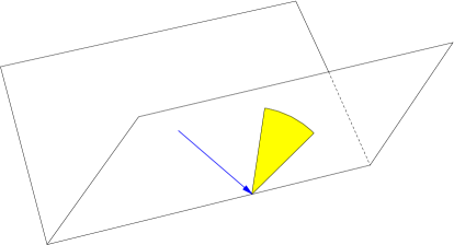
Figure 1. A ray carrying a singularity may strike a corner of codimension two and give rise to a whole family of diffracted singularities, conserving both energy and momentum along the corner.

The first diffraction problem to be rigorously treated was that of the exterior of a wedge, which was analyzed by Sommerfeld [Sommerfeld1]; subsequently, many related examples were analyzed by Friedlander [MR20:3703], and more generally the case of exact cones was worked out explicitly by Cheeger-Taylor [Cheeger-Taylor2], [Cheeger-Taylor1] in terms of the functional calculus for the Laplace operator on the cross section of the cone. All of these explicit examples reveal that generically a diffracted wave arises from the interaction of wavefront set of the solution with singular strata of the boundary of the manifold; this has long been understood at a heuristic level, with the geometric theory of diffraction of Keller [Keller1] describing the classes of trajectories that ought to contribute to the asymptotics of the solution in various regimes.

Subsequent work has been focused primarily on characterizing the bicharacteristics on which singularities can propagate, and on describing the strength and form of the singularities that arise. The propagation of singularities on manifolds with boundary was first understood in the analytic case by Sjöstrand [Sjostrand3, Sjostrand2, Sjostrand4], and subsequently generalized to a very wide class of manifolds, including manifolds with corners, by Lebeau [Lebeau4, Lebeau5]. In the $\mathcal{C}^{\infty}$ setting employed here, the special case of manifolds with conic singularities was studied by Melrose-Wunsch [Melrose-Wunsch1] and edge manifolds (i.e., cone bundles) were considered by Melrose-Vasy-Wunsch [mvw1]. Vasy [Vasy5] obtained results analogous to Lebeau’s in the case of manifolds with corners, and it is the results of this work that directly bear on the situation studied here.

While the foregoing results characterize which bicharacteristics may carry singularities for solutions to the wave equation, they ignore the question of the regularity of the diffracted front. In general, a singularity in $\operatorname{WF}^{s}$ (which is to say, measured with respect to $H^{s}$) must propagate strongly in the sense that some bicharacteristics through the point in question must also lie in $\operatorname{WF}^{s}.$ The general expectation is that these are certain “geometric” bicharacteristics; in simple cases, these are known to be those which are locally approximable by bicharacteristics that miss the corners and reflect transversely off boundary hypersurfaces. More generally, we can define geometric bicharacteristics as follows: To begin, we blow up the corner, i.e. introduce polar coordinates around it; this serves to replace the corner with its inward-pointing normal bundle, which fibers over the corner with fiber given by one orthant of a sphere, $S^{f}\cap(\mathbb{R}^{+})^{f+1}.$ We will define geometric broken bicharacteristics passing through the corner as those that lift to the blown-up space to enter and leave the lift of the corner at points connected by generalized broken geodesics of length $\pi$ with respect to the naturally defined metric on $S^{f}\cap(\mathbb{R}^{+})^{f+1},$ undergoing specular reflection at its boundaries and corners. Bicharacteristics that enter and leave the corner at points in a fiber that are not at distance-$\pi$ in this sense are referred to as “diffractive.” See Figure 2.

Figure 2. Geometric optic rays hitting a corner $F$, emanating from a point $o$. The rays labelled $G$ are geometric at $F$, while those labelled $NG$ are non-geometric at $F$. The leftmost geometric ray is a limit of rays like the unlabelled one shown on the figure that just miss $F$. The blown up version of the picture, i.e. where $(r,\theta)$ are introduced as coordinates at the origin, is shown on the right. The front face (i.e., the lift of the corner) is denoted $\operatorname{ff}.$ The reflecting line indicates the broken geodesic of length $\pi$ induced on $\operatorname{ff}$ given by $r=0$, $\theta\in[0,\theta_{0}]$. The total length of the three segments shown on $\operatorname{ff}$ is $\pi$; this can be thought of as the sum of three angles on the picture on the left: namely the angles between the incident ray and the right boundary (corresponding to the first segment), the right and left boundaries, finally the left boundary and the emanating reflected ray.

It turns out that subject to certain hypotheses of nonfocusing, the singularities propagating along diffractive bicharacteristics emanating from the corner will be weaker than those on geometric bicharacteristics. In particular, the fundamental solution satisfies the nonfocusing condition, hence one consequence of our main theorem is as follows:

Theorem 1.1.

Consider the fundamental solution $u_{o}$ to the wave equation, with pole $o$ sufficiently close to a corner, $Y,$ of codimension $k.$ Assume that $o$ is sufficiently far from the boundary that every short geodesic from $o$ to $Y$ is transverse to all boundary hypersurfaces intersecting at $Y.$

While $u_{o}$ lies locally in $H^{-n/2+1-0},$ it is less singular by $(k-1)/2$ derivatives along diffractive bicharacteristics emanating from $Y,$ that is, it lies microlocally in $H^{(-n+k+1-0)/2}$ there.

A more precise version of this result (with “sufficiently close…” elucidated) appears in Corollary 9.8.

A more general theorem on regularity of the diffracted wave subject to the nonfocusing condition is the central result of this paper. See §1.2 for a rough statement of the nonfocusing condition and §6 for technical details; the main theorem is stated and proved in §9.

There are a few related results known in special cases. Gérard-Lebeau [MR93f:35130] explicitly analyzed the problem of an analytic conormal wave incident on an analytic corner in $\mathbb{R}^{2},$ obtaining a $1/2$-derivative improvement of the diffracted wavefront over the incident one. The first and third authors [Melrose-Wunsch1] obtained corresponding results for manifolds with conic singularities, which the authors subsequently generalized to the case of edge manifolds [mvw1].

We remark that our definition of geometric broken bicharacteristics includes those that interact with the boundaries and corners of the front face of the blow-up, $S^{f}\cap(\mathbb{R}^{+})^{f+1},$ according to the simplest laws of reflection as described in [Vasy5]: we do not distinguish between “diffractive” and “geometric” interactions within $S^{f}\cap(\mathbb{R}^{+})^{f+1}.$ We conjecture that a stronger theorem than ours should hold in which, instead of simply blowing up the highest-codimension corner, we might iteratively blow up the corners of lower codimension as well. This would enable us to (iteratively) distinguish bicharacteristics that undergo diffractive or geometric interaction inside the faces of the blown-up space. For instance, in the case of a codimension-$3$ corner, such a method would distinguish among rays that are limits of families of geodesics undergoing simple specular reflection with boundary hypersurfaces (which we might continue to call geometric rays); limits of families which undergo a single diffractive interaction with a codimension-$2$ corner (partially diffractive rays) and all other generalized broken bicharacteristics entering and leaving the codimension-$3$ corner (the completely diffractive rays). Our Theorem 1.1 only deals with the regularity along the completely diffractive rays, telling us that the fundamental solution is $(3-1)/2$ derivatives smoother along them than overall; the conjectural finer result would also tell us about the partially diffractive rays, yielding an improvement of $(2-1)/2$ derivatives there. More generally, such a result ought to yield a stratification of the rays interacting with a corner of arbitrary codimension into pieces carrying different levels of differentiability according to the degree of diffractive interaction.

1.2. The hypothesis

We now describe the nonfocusing hypothesis in more detail, in the context of the simplest geometric situation to which our results apply.

It is easily seen from the explicit form of the fundamental solution that it is not in general true that diffracted rays are more regular than incident singularities. For example, take $\varDelta$ to be the Dirichlet Laplacian in a sectorial domain $\{r\in[0,\infty),\theta\in[0,\theta_{0}]\}$ in $\mathbb{R}^{2},$ and consider the solution

(1.2) $$\frac{\sin t\sqrt{\varDelta}}{\sqrt{\varDelta}}\phi(\theta)\delta(r-r_{0}),$$

where $\phi\in\mathcal{C}_{c}^{\infty}((0,\theta_{0}))$ is supported close to some value $\theta^{\prime}.$ This solution is manifestly locally in $H^{1/2-0}$ by energy conservation. On the other hand one may see from the explicit form of the propagator in [Cheeger-Taylor2], [Cheeger-Taylor1] after convolution with $\phi(\theta)$ that a spherical wave of singularities emanates from the corner at time $t=r_{0},$ with regularity $H^{1/2-0},$ hence the same as the overall Sobolev regularity of the solution. The bicharacteristics along which singularities propagate are, for short time, just the lifts of the straight lines $r=r_{0}\pm t,$ $\theta\in\operatorname{supp}\phi,$ hence travelling straight into or out of the vertex. Perturbing these slightly to make them miss the vertex, we see that in fact there are two “geometric” continuations for each bicharacteristic, depending on whether we approximate it by geodesics passing to the left or to the right of the vertex (see Figure 2). Thus, the geometric continuations of the rays on which singularities strike the vertex are close to the two possible continuations of the single ray $\theta=\theta^{\prime},$ hence do not include all points on the outgoing spherical wave. So we have an example in which there are “non-geometric” singularities of full strength.

The nonfocusing condition serves exactly to rule out such situations. The above example has the property that applying negative powers of $(\operatorname{Id}+D_{\theta}^{2})$ does not regularize the short-time solution (or the initial data) as it is already ${\mathcal{C}}^{\infty}$ in the $\theta$ direction. In this simple setting, the nonfocusing condition says precisely that the solution is regularized by negative powers of $(\operatorname{Id}+D_{\theta}^{2}),$ or, equivalently, that it can be written

$$(\operatorname{Id}+D_{\theta}^{2})^{N}v,\ v\in H^{s}$$

for some $s$ exceeding the overall Sobolev regularity. For instance, the fundamental solution

$$u=\frac{\sin t\sqrt{\varDelta}}{\sqrt{\varDelta}}\delta(r-r^{\prime})\delta(\theta-\theta^{\prime})$$

looks, after application of a sufficiently negative power of $(\operatorname{Id}+D_{\theta}^{2}),$ like a distribution of the form

$$\frac{\sin t\sqrt{\varDelta}}{\sqrt{\varDelta}}\delta(r-r^{\prime})f(\theta)$$

with $f\in\mathcal{C}^{M},$ $M\gg 0,$ hence we can write

$$u\in(\operatorname{Id}+D_{\theta}^{2})^{N}H^{1/2-0},$$

for some $N\gg 0,$ at least locally, away from the boundary. We also observe that the example (1.2) enjoys a property which is essential dual to the nonfocusing condition, to wit, fixed regularity under repeated application of $D_{\theta}.$ We refer to this property as “coisotropic regularity” (the terminology will be explained in §6) and it plays an essential role in our proof.

The nonfocusing condition and coisotropic regularity in a more general setting are subtler owing to their irreducibly microlocal nature: the operator $D_{\theta}$ has to be replaced by a family of operators characteristic along the flow-out of the corner under consideration.

1.3. Structure of the proof

We now describe the logical structure of the proof, as it is somewhat involved. The heart of the argument is a series of results on the propagation of singularities, obtained by positive commutator methods; these are sketched in detail in §1.4 below. In order to be able to distinguish between “geometric” and “diffractive” bicharacteristics at a corner of $M_{0},$ we begin by performing a blow-up of the corner, i.e. introducing polar coordinates centered at it, to obtain a new manifold with corners $M.$ The commutants that we employ in our commutator argument almost lie in a calculus of pseudodifferential operators, the edge-b calculus, that behaves like Mazzeo’s edge calculus [MR93d:58152] near the new boundary face introduced by the blow-up (henceforth, the edge) and like Melrose’s b calculus [MR83f:58073, Melrose:Atiyah, Melrose-Piazza:Analytic] at the remaining boundary faces. The complication, as in the previous work of Vasy [Vasy5] on propagation of singularities, is that in order to control certain error terms we in fact must employ a hybrid differential-pseudodifferential calculus, in which we keep track of certain terms involving differential operators normal to the boundary faces other than $\tilde{W}.$

Even this propagation result alone is insufficient to obtain our result, as it does not allow regularity of greater than a certain degree to propagate out of the edge, with the limitation in fact not exceeding the a priori regularity of the solution. What it does allow for, however, is the propagation of coisotropic regularity of arbitrarily high order, suitably microlocalized in the edge-b sense. This allows us to conclude that given a ray $\gamma$ leaving the edge, if the solution enjoys coisotropic regularity along all rays incident upon the edge that are geometrically related to $\gamma$, then we may conclude coisotropic regularity along $\gamma$ as well. (If some of these incident rays are glancing, i.e. tangent to the boundary, we require as our hypothesis actual differentiability globally at all incoming glancing rays rather than coisotropic regularity, which no longer makes sense; the version of the commutator argument that deals with these rays is the most technically difficult aspect of the argument.) In particular, then, global coisotropic regularity together with ${\mathcal{C}}^{\infty}$ regularity at glancing rays implies global coisotropic regularity leaving the edge away from glancing. We are then able to dualize this result to show that the nonfocusing condition propagates as well.

Consequently, we show that subject to the nonfocusing condition, in the model case of the sector considered above, if $\gamma$ is an outgoing ray such that the solution is ${\mathcal{C}}^{\infty}$ along all incoming rays geometrically related to it,

$$u\in(\operatorname{Id}+D_{\theta})^{N}H^{s}\text{ along }\gamma\text{ for some }N\in\mathbb{N},$$

where in general $s=(-n+k+1)/2-0$ for the fundamental solution near a codimension-$k$ corner on an $n$-manifold, hence $s=1/2-0$ for the sector. On the other hand the microlocal propagation of coisotropic regularity shows that

$$D_{\theta}^{k}u\in H^{s_{0}}\text{ for all }k\text{ along }\gamma$$

where $s_{0}$ is the overall regularity of the solution ($-n/2+1-0$ for the fundamental solution). An interpolation argument then yields

$$u\in H^{s-0}\text{ along }\gamma,$$

proving the theorem.

1.4. Sketch of the propagation results

We now discuss the propagation results in greater detail, focusing on the taxonomy of the various spaces of operators that we employ. The basic propagation of singularities result on manifolds with corners $M_{0}=\mathbb{R}_{t}\times X_{0}$, as on manifolds with smooth boundaries, is in the setting of b-, or totally characteristic, operators. Let us choose local coordinates $(x_{1},\ldots,x_{f+1},y_{1},\ldots,y_{n-f-1})$ on $X_{0}$ with $\{x_{1}\geq 0,\ldots,x_{f+1}\geq 0\};$ thus, $Y=\{x_{1}=\ldots=x_{f+1}=0\}$ represents a corner of codimension $f+1.$ The b-vector fields $\mathcal{V}_{\operatorname{b}}(X_{0})$ are the linear combinations of $x_{j}\partial_{x_{j}}$ and $\partial_{y_{j}}$ with ${\mathcal{C}}^{\infty}$ coefficients—these are exactly the vector fields tangent to all boundary hypersurfaces. We can define an associated notion of b-regularity by iterated regularity under repeated application of such vector fields. In particular, for a distribution $u$, b-regularity relative to a space, such as $H^{1}(X_{0})$, means that $(x\partial_{x})^{\alpha}\partial_{y}^{\beta}u\in H^{1}(X_{0})$ for all multiindices $\alpha,\beta$ (with $(x\partial_{x})^{\alpha}=(x_{1}\partial_{x_{1}})^{\alpha_{1}}\ldots(x_{f+1}\partial_{x_{f+1}})^{\alpha_{f+1}}$). Thus $u$ is b-regular if and only if $u$ is a conormal distribution. Replacing $X_{0}$ by $M_{0}$ simply adds $\partial_{t}$ to the collection of b-vector fields, i.e. $t$ behaves as one of the $y$ variables. The notion of b-regularity is microlocalized via the b-pseudodifferential operators, which are roughly speaking operators of the form $a(x,y,t,xD_{x},D_{y},D_{t})$ where $a$ is a symbol in the last three sets of variables. The calculus of these operators gives rise to a notion of b-wavefront set, which is therefore a microlocal measure of conormality.

The wave operator itself is not a b-differential operator, rather a standard differential operator: it is constructed out of the vector fields $\partial_{x_{j}}$ rather than $x_{j}\partial_{x_{j}}$. Thus, its principal symbol, hence its bicharacteristics, are curves in the cotangent bundle $T^{*}M_{0}$, which is equipped with canonical coordinates $(x,y,t,\xi^{\operatorname{s}},\eta^{\operatorname{s}},\tau^{\operatorname{s}})$, corresponding to differential operators $(x,y,t,D_{x},D_{y},D_{t})$. One cannot work with pseudodifferential operators based on these standard differential operators, for they would usually not act on smooth functions in $x\geq 0$, and would not usually preserve the boundary conditions. Thus, one works with b-operators, based on $(x,y,t,xD_{x},D_{y},D_{t})$, which corresponds to localizing in conic neighborhoods in the corresponding canonical coordinates $(x,y,t,\xi^{\operatorname{b}},\eta^{\operatorname{b}},\tau^{\operatorname{b}})$ in the cotangent bundle. These coordinates are related to the original ones via

$$(x,y,t,\xi^{\operatorname{b}},\eta^{\operatorname{b}},\tau^{\operatorname{b}})=(x,y,t,x\xi^{\operatorname{s}},\eta^{\operatorname{s}},\tau^{\operatorname{s}}).$$

In particular, at $x=0$, passing to the b-coordinates identifies points with different values of the normal momentum $\xi^{\operatorname{s}}.$ Continuous propagation in the b-variables thus allows $\xi^{\operatorname{s}}$ to jump at the boundary, as occurs in specular reflection. It is the phenomenon of propagation along appropriate generalized bicharacteristics in the b-variables that was studied in [Vasy5].

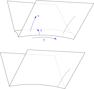
Figure 3. A manifold $X_{0}$ with corners of codimension two (below) and its blow-up $X$ (top). A geodesic hitting the codimension-two corner is shown, together with its lift to the blown-up space $X,$ which then strikes the front “edge” face of the blow-up.

In order to have a more precise result, we need to be able to localize within the fibers of the blow-up of the corner $Y$, and we also need to be able to undo the compression of the dynamics implied by working in the b-picture. It is only through these refinements that we are able to distinguish microlocal behavior along different bicharacteristics hitting the corner $Y$ at the same point and with the same tangential momenta $\eta^{\operatorname{b}},$ e.g. between different geodesics in the conical spray shown leaving the corner in Figure 1. Therefore we lift the Laplacian on $X_{0}$ to the blow-up $X$ of $X_{0}$ at $Y$, denoted $X=[X_{0};Y]$. For simplicity of notation, assume that $Y$ is a codimension $2$ corner (cf. Figure 2 as well as Figure 3 below). Using polar coordinates $(r,\theta)$ in the $(x_{1},x_{2})$ we see that under this blow-up smooth vector fields on $X$ lift to vector fields of the form $r^{-1}V$, where $V$ is tangent to the fibers of the blow-down map, i.e. is a linear combination of $r\partial_{r},\partial_{\theta},r\partial_{y}$ with ${\mathcal{C}}^{\infty}$ coefficients. The ${\mathcal{C}}^{\infty}$ span of $r\partial_{r},\partial_{\theta},r\partial_{y}$ are the so-called edge-smooth vector fields defined below in Section 3. Away from the boundaries, $\theta=0,\pi/2$ in $[0,\pi/2]_{\theta}$, these are exactly the edge vector fields introduced by Mazzeo [MR93d:58152] on manifolds with smooth boundaries. Here the fibers have boundaries (in our example, the fibers are just the interval $[0,\pi/2]_{\theta}$), and smoothness is required up to these boundaries. A key observation is that the wave operator lifts to an edge-smooth differential operator on $M=\mathbb{R}_{t}\times X$.

Propagation phenomena in the edge setting (when the fibers have no boundaries) have been treated in [mvw1], following [Melrose-Wunsch1]. We now recall these results, as they apply in the setting discussed here, provided we stay away from the fiber boundaries. We emphasize that in the edge picture both the operator one studies (the wave operator) and the microlocalizers are edge pseudodifferential operators, i.e. there is no need to use two different algebras as in the manifolds with corners setting discussed above. In order to avoid complicating the notation, we simply replace $[0,\pi/2]_{\theta}$ by the circle; edge operators are then formally of the form $a(r,\theta,y,t,rD_{r},D_{\theta},rD_{y},rD_{t})$. Writing covectors as $\underline{\xi}\,\frac{dr}{r}+\underline{\zeta}\,d\theta+\underline{\eta}\,\frac{dy}{r}+\underline{\tau}\,\frac{dt}{r}$, their symbols are thus smooth functions of $(r,\theta,y,t,\underline{\xi},\underline{\zeta},\underline{\eta},\underline{\tau})$; in the setting of classical operators they are homogeneous in the last three sets of variables. In particular, the principal symbol of the wave operator is such a symbol, and its Hamilton vector field is a smooth homogeneous vector field in these coordinates. Its dynamical system in the characteristic set governs the analysis of solutions; by homogeneity, it is convenient to study these dynamics in the corresponding cosphere bundle. Then there are two (incoming, resp. outgoing) sets of critical points over $r=0$, corresponding to radial points of the Hamilton vector field. These are both saddle manifolds, with either the stable or the unstable manifold for each of these contained in the boundary face $r=0$, and the other transversal to it. The Hamilton flow within $r=0$ connects the incoming and outgoing radial sets, and fixes the “slow variables” $(y,t,\underline{\eta}/\underline{\tau})$ (with the last variable projectivized to work on the cosphere bundle); the projection of its integral curves to the base variables gives the distance $\pi$ propagation of the geometric theorem of [mvw1]. One should thus picture singularities entering the boundary $r=0$ along (say) the stable manifold of one of these critical manifolds, propagating through the critical manifold and out through its unstable manifold; propagating across the boundary to the stable manifold of the other critical manifold; and then through it and back out of the boundary along the corresponding unstable manifold. As this whole process leaves the slow variables unaffected, we see that they are preserved under the interaction with the boundary, leading to the law of specular reflection.

To make sense of the propagation described above, one thus needs to have a description of propagation at incoming and outgoing radial points, as well as elsewhere within $r=0$; this was accomplished in [mvw1]. It is the radial points that cause the most significant subtleties in the propagation of singularities: at these points the relation generated by the flow becomes multi-valued, as in general a singularity arriving at a critical point along its stable manifold may produce singularities leaving along the whole unstable manifold. An important part of the analysis is to note that at the radial points, coisotropy corresponding to the stable/unstable submanifold transversal to $r=0$ implies regularity (absence of edge wave front set) in the unstable/stable manifold within $r=0$, and conversely. In particular, an incident wave coisotropic for the flow-in becomes edge-regular within $r=0$ (away from the radial points) and then emerges to be coisotropic for the flow-out. A slight complication is that coisotropy is relative to a function space; there are losses in the background regularity space due to the radial points.

The added difficulty in our setting relative to that of [mvw1] is that the fibers have boundaries, and indeed typically corners. We deal with this by treating the propagation into and out of these corners inside $r=0$ analogously to the propagation of b-regularity analyzed in [Vasy5]. We thus compress the edge-smooth cotangent bundle, essentially by replacing the “smooth” vector field $\partial_{\theta}$ by one tangent to the boundaries of the fibers, i.e., using $f(\theta)\partial_{\theta}$ instead, where $f(\theta)=\sin\theta\cos\theta$ has simple zeros at $\theta=0$, $\theta=\pi/2$ and is non-zero elsewhere in $[0,\pi/2]$. Note that $r\partial_{r}$, $r\partial_{y}$ and $r\partial_{t}$ are already tangent to the boundary faces $\theta=0,\pi/2$, so they do not require any adjustments. The resulting vector fields are thus those tangent to the fibers of the front face of the blow-up, as well as to all other boundary faces, and we call these edge-b vector fields. We use a pseudodifferential algebra $\Psi_{\operatorname{eb}}^{*}(M)$ microlocalizing these vector fields to prove our main results. In addition to the already discussed results away from the boundaries of the fibers, we thus need to analyze propagation at incoming and outgoing radial points at the boundaries of the fibers, as well as the analogue of hyperbolic and glancing points in the setting of $M_{0}$. This is accomplished in Section 7.

Note that conormal regularity in $X_{0}$ near a point is equivalent, after blow-up, to conormal regularity near the corresponding fiber of the front face. Explicitly, in our example of a codimension $2$ corner, regularity with respect to $x_{1}\partial_{x_{1}},x_{2}\partial_{x_{2}}$ and $\partial_{y}$ is equivalent to regularity with respect to $r\partial_{r}$, $f(\theta)\partial_{\theta}$ and $\partial_{y}$, where $f(\theta)=\sin\theta\cos\theta$. Thus, away from $\theta=0,\pi/2$, i.e., in the interior of the front face, one has regularity with respect to $r\partial_{r}$, $\partial_{\theta}$ and $\partial_{y}$—where that this notion of regularity ignores the fibration. Edge regularity in the same region is with respect to $r\partial_{r}$, $\partial_{\theta}$ and $r\partial_{y}$, i.e., it is a weaker notion than conormality. However, the ability to microlocalize within the fibers depends on its use.

1.5. Organization of the paper

We start in Section 2 by describing the blown-up space on which our analysis takes place. Then, in Section 3, we describe in detail the connection between both the smooth and b-structures on $M_{0}$, and between the edge-smooth and edge-b structures on $M$. In the same section, we study the bicharacteristics in the edge-b setting, i.e. that of $M$; this is in many respects analogous to Lebeau’s work [Lebeau5] in the blown-down setting (e.g. on $M_{0}$), though radial points are an important new feature.

In Section 4, with the operator algebra construction provided by Appendix B, we describe edge-b pseudodifferential operators, and then in Section 5 the algebra of operators that are both edge-smooth-differential and edge-b-pseudodifferential; these provide the link between the wave operator (which is edge-smooth) and the microlocalizers (which are edge-b). The use of this mixed differential-pseudodifferential calculus is analogous to the use of (smooth-)differential, tangential-pseudodifferential operators by Melrose-Sjöstrand [Melrose-Sjostrand1, Melrose-Sjostrand2] in the smooth boundary setting, and (smooth-)differential, b-pseudodifferential operators in [Vasy5] in the proof of the standard propagation result on manifolds with corners. This calculus provides the framework for the positive commutator estimates proving the edge-b propagation results. In Section 6 we discuss coisotropic distributional, and their dual, non-focusing, spaces. Section 7 proves the edge-b propagation of singularities. In Section 8 we show how coisotropy propagates through the edge. Finally, in Section 9 we prove the main theorem, Theorem 9.6, and its corollaries, which in particular imply Theorem 1.1.

To ease the notational burden on the reader, an index of notation is provided at the end of the paper.

1.6. Acknowledgements

The authors gladly acknowledge the support of the National Science Foundation under grants DMS-0408993 (RM), DMS-0733485 and DMS-0801226 (AV) and DMS-0700318 (JW). The second author was also supported by a Chambers Fellowship from Stanford University. All three authors are grateful to MSRI for both support and hospitality in the fall of 2008, during which the bulk of this manuscript was written. Two anonymous referees contributed many helpful suggestions and corrections to the exposition.

2. Geometry: metric and Laplacian

Let $X_{0}$ be a connected $n$-dimensional manifold with corners. We work locally, near a given point in the interior of a corner $Y$ of codimension $f+1.$ Thus, we have local coordinates $x_{1},\ldots,x_{f+1},y_{1},\ldots,y_{n-f-1}$ in which $Y$ is given by $x_{1}=\ldots=x_{f+1}=0$. Suppose that $g_{0}$ is a smooth Riemannian metric on $X_{0},$ non-degenerate up to all boundary faces. We may always choose local coordinates in which it takes the form

(2.1) $$g_{0}=\sum a_{ij}\,dx_{i}\,dx_{j}+\sum b_{ij}\,dy_{i}\,dy_{j}+2\sum c_{ij}\,dx_{i}\,dy_{j}$$

with $c_{ij}|_{Y}=0.$ This can be arranged by changing the $y$ variables to

$$y_{j}=y^{\prime}_{j}+\sum x_{k}Y_{jk}(y^{\prime})$$

while keeping the $x_{j}$ unchanged. The cross-terms then become

$$2\sum c_{ij}\,dx_{i}\,dy^{\prime}_{j}+2\sum b_{ij}\,Y_{jk}\,dy^{\prime}_{i}\,dx_{k},$$

which can be made to vanish by making the appropriate choice of the $Y_{jk},$ using the invertibility of $\{b_{ij}\}.$

Let $X=[X_{0};Y],$ be the real blow-up of $Y$ in $X_{0}$ (see [Melrose:Atiyah, MR95k:58168]) and let $\tilde{Y}$ denote the front face of the blow-up, which we also refer to as the edge face. Recall that the blow-up arises by identifying a neigborhood of $Y$ in $X_{0}$ with the inward-pointing normal bundle $N^{+}Y$ of $Y$ in $X_{0}$ and blowing up the origin in the fibers of the normal bundle (i.e. introducing polar coordinates in the fibers). Since the normal bundle is trivialized by the defining functions of the boundary faces, a neighborhood of $\tilde{Y}$ in $X$ is globally diffeomorphic to

$$[0,\infty)\times Y\times Z,\ \text{where}\ Z=S^{f}\cap[0,\infty)^{f+1}.$$

We use coordinates $z_{1},\dots,z_{f}$ in $Z;$ near a corner of $Z$ of codimension $k,$ these are divided into $z^{\prime}_{1},\dots,z^{\prime}_{k}\in[0,\infty)$ and $z^{\prime\prime}_{k+1},\dots,z^{\prime\prime}_{f}\in\mathbb{R}.$ There is significant freedom in choosing the identification of a neighborhood of $Y$ and the coordinates on the fibers of the normal bundle but the naturality of the smooth structure on the blown up manifold, $[X_{0};Y],$ corresponds to the fact that these are smoothly related.

The metric $g_{0}$ identifies $NY$ as a subbundle of $T_{Y}X_{0}.$ This corresponds to coordinates $(x_{i},y_{j})$ as above with the $dy_{j}$ orthogonal to $dx_{i}$ at $Y.$ In the blow-up polar coordinates are introduced in the $x_{i}$ but the $y_{j}$ are left unchanged. It is convenient to think of these as polar coordinates induced by $\sum_{ij}a_{ij}\,dx_{i}\,dx_{j}.$ In particular, we choose

$$x=\Big{(}\sum_{ij}a_{ij}(0,y)x_{i}x_{j}\Big{)}^{1/2}$$

as the ‘polar variable’ which is the defining function of the front face. With this choice, the metric takes the form

(2.2) $$g=dx^{2}+h(y,dy)+x^{2}k(x,y,z,dz)+xk^{\prime}(x,y,z,dx,dy,x\,dz).$$

More generally, one can simply consider the wider class of manifolds with corners with metrics of the form (2.2), we refer to these as ‘edge metrics’ for brevity. Note, however, that there are no results currently available in this wider setting that limit propagation of singularities to generalized broken bicharacteristics. Despite this, the results in §7 remain valid in this more general context.

Now, set

$$M=\mathbb{R}_{t}\times X,\ M_{0}=\mathbb{R}\times X_{0},\ \tilde{W}=\mathbb{R}\times\tilde{Y},\ W=\mathbb{R}\times Y,$$

where $W$, resp. $\tilde{W}$ now represent the unresolved, resp. blown-up, version of the space-time “edge.”

Let $\operatorname{Diff}^{*}_{\operatorname{es}}(X)$ denote the filtered algebra of operators on ${\mathcal{C}}^{\infty}(X)$ generated by those vector fields that are tangent to the fibers of the front face $\tilde{Y}$ produced by the blow up; $xD_{x},$ $xD_{y_{j}},$ $D_{z_{j}}$ form a local coordinate basis of these vector fields. See §3 and §5 for further explanation of this algebra and of our terminology. The same definition leads to the algebra of operators $\operatorname{Diff}^{*}_{\operatorname{es}}(M)$ on ${\mathcal{C}}^{\infty}(M)$ with local generating basis $xD_{t},$ $xD_{x},$ $xD_{y_{j}},$ $D_{z_{j}}.$

Lemma 2.1.

The Laplace operator $\varDelta\in x^{-2}\operatorname{Diff}^{2}_{\operatorname{es}}(X)$ on $X$ is of the form

$$\varDelta\in D_{x}^{2}+\frac{f}{\imath x}D_{x}+\frac{1}{x^{2}}\varDelta_{Z}+\varDelta_{Y}+x^{-1}\operatorname{Diff}^{2}_{\operatorname{es}}(X)$$

where $\varDelta_{Z}$ is the Laplace operator in $Z$ with respect to the metric $h$ (and hence depends parametrically on $x$ and $y)$ and $\varDelta_{Y}$ is the Laplacian on $Y$ with respect to the metric $k.$

In particular, ${\square}=D_{t}^{2}-\Delta_{X}\in x^{-2}\operatorname{Diff}^{2}_{\operatorname{es}}(M)$.

3. Bundles and bicharacteristics

In this section, we discuss several different geometric settings in which the propagation problem for ${\square}$ on $M_{0}$ may be viewed. Somewhat loosely, each of these corresponds to a choice of a Lie algebra of vector fields with different boundary behavior; these then lead to distinct bundles of covectors, with the corresponding descriptors used as section headings here. The first, the “b”-bundle, can be considered either on $M_{0}$ or $M.$ Indeed, the bundle of b-covectors on $M_{0}$ is the setting for the propagation results of [Vasy5]: these results are, as will be seen below, necessarily global in the corner, and do not distinguish between general diffractive rays and the subset of geometric rays (defined below). In order to discuss the improvement in regularity which can occur for propagation along the geometric rays, two more bundles of covectors, lying over the blown-up space $M,$ are introduced. These, the “edge-b” and “edge-smooth” bundles, keep track of local information in the fibers of the blow-up $\tilde{W}$ of $W$ in $M_{0},$ and allow us to distinguish the diffractive rays from geometric ones. The distinction between the edge-b and edge-smooth bundles comes only at the boundary of $\tilde{W},$ and the relationship between the two bundles gives rise to reflection of singularities off boundary faces, uniformly up to the edge $\tilde{W}.$

In order to alleviate some of the notational burden on the reader, a table is included in §3.5 in which the various bundles, their coordinates, their sections, and some of the maps among them are reviewed. The standard objects for a manifold with corners, $Q,$ correspond to uniform smoothness up to all boundary faces, so $\mathcal{V}(Q)$ denotes the Lie algebra of smooth vector fields, $TQ,$ the tangent bundle, of which $\mathcal{V}(Q)$ forms all the smooth sections, $T^{*}Q$ is its dual, etc.

3.1. b-Cotangent bundle

Let $\mathcal{V}_{\operatorname{b}}(Q)\subset\mathcal{V}(Q)$ denote the Lie subalgebra of those smooth vector fields on the general manifold with corners $Q,$ which are tangent to each boundary face. If we choose coordinates as in §3, the local vector fields

$$x_{1}\partial_{x_{1}},\dots,x_{f+1}\partial_{x_{f+1}},\partial_{y_{1}},\dots,\partial_{y_{n-f-1}};$$

form a basis over smooth functions. Hence $\mathcal{V}_{\operatorname{b}}(Q)$ is the space of ${\mathcal{C}}^{\infty}$-sections of a vector bundle, denoted

$${}^{\operatorname{b}}TQ.$$

The dual bundle ${}^{\operatorname{b}}T^{*}Q$ therefore has sections spanned by

$$\frac{dx_{1}}{x_{1}},\dots,\frac{dx_{f+1}}{x_{f+1}},d{y_{1}},\dots,d{y_{n-f-1}}.$$

The natural map

(3.1) $$\pi_{\operatorname{s}\to\operatorname{b}}:T^{*}Q\longrightarrow{}^{\operatorname{b}}T^{*}Q$$

is the adjoint of the bundle map $\iota:{}^{\operatorname{b}}TQ\to TQ$ corresponding to the inclusion of $\mathcal{V}_{\operatorname{b}}(Q)$ in $\mathcal{V}(Q).$

Canonical local coordinates on $T^{*}M_{0}$ correspond to decomposing a covector in terms of the basis as

$$\tau^{\operatorname{s}}\,dt+\sum_{j}\eta^{\operatorname{s}}_{j}\,dy_{j}+\sum_{j}\xi^{\operatorname{s}}_{j}\,dx_{j},$$

and elements of ${}^{\operatorname{b}}T^{*}M_{0}$ may be written

$$\tau^{\operatorname{b}}\,dt+\sum_{j}\eta^{\operatorname{b}}_{j}\,dy_{j}+\sum_{j}\xi^{\operatorname{b}}_{j}\,\frac{dx_{j}}{x_{j}},$$

so defining canonical coordinates. The map (3.1) then takes the form

$$\pi_{\operatorname{s}\to\operatorname{b}}(x,y,t,\xi^{\operatorname{s}},\eta^{\operatorname{s}},\tau^{\operatorname{s}})=(x,y,t,\xi^{\operatorname{b}},\eta^{\operatorname{b}},\tau^{\operatorname{b}})=(x,y,t,x\xi^{\operatorname{s}},\eta^{\operatorname{s}},\tau^{\operatorname{s}}),$$

with $x\xi^{\operatorname{s}}=(x_{1}\xi^{\operatorname{s}}_{1},\ldots,x_{f+1}\xi^{\operatorname{s}}_{f+1}).$

The setting for the basic theorem on the propagation of singularities in [Vasy5] is ${}^{\operatorname{b}}T^{*}M_{0}.$ In particular, generalized broken bicharacteristics, or GBBs, are curves in ${}^{\operatorname{b}}T^{*}M_{0}.$ In order to analyze the geometric improvement, spaces that will keep track of finer singularities are needed. Before introducing these, we first recall the setup for GBBs. Note that at $W,$ $\pi_{\operatorname{s}\to\operatorname{b}}|_{W}$ maps $N^{*}W$ onto the zero section over $W,$ and is injective on complementary subspaces of $T^{*}_{W}M_{0}$, so we may make the identification

$$\pi_{\operatorname{s}\to\operatorname{b}}|_{W}(T^{*}_{W}M_{0})\cong T^{*}W.$$

We also recall that it is convenient to work on cosphere bundles. Since it is linear, $\pi_{\operatorname{s}\to\operatorname{b}}$ intertwines the $\mathbb{R}^{+}$-actions, but it does not induce a map on the corresponding cosphere bundles since it maps part of $T^{*}M_{0}\setminus o$ into the zero section of ${}^{\operatorname{b}}T^{*}M_{0}.$ However, on the characteristic set of ${\square}$ this map is better behaved. Let

$$p_{0}=\sigma_{2}({\square})\in{\mathcal{C}}^{\infty}(T^{*}M_{0}\setminus o)$$

be the standard principal symbol of ${\square}\in\operatorname{Diff}^{2}(M_{0});$ it is of the form

$$p_{0}=(\tau^{\operatorname{s}})^{2}-\Big{(}\sum A_{jk}\xi^{\operatorname{s}}_{j}\xi^{\operatorname{s}}_{k}+\sum B_{jk}\eta^{\operatorname{s}}_{j}\eta^{\operatorname{s}}_{k}+2\sum C_{jk}\xi^{\operatorname{s}}_{j}\eta^{\operatorname{s}}_{k}\Big{)}$$

with $A_{jk},B_{jk},C_{jk}\in{\mathcal{C}}^{\infty}(M_{0})$, $A_{jk}=A_{kj}$ and $B_{jk}=B_{kj},$ $C_{jk}|_{x=0}=0.$ Let

(3.2) $${}^{\operatorname{s}}\Sigma_{0}=p_{0}^{-1}(\{0\})/\mathbb{R}^{+}\subset S^{*}M_{0}$$

be the spherical image of the characteristic set of ${\square}.$ This has two connected components, ${}^{\operatorname{s}}\Sigma_{0,\pm},$ corresponding to $\tau^{\operatorname{s}}\gtrless 0$ since $\{\tau^{\operatorname{s}}=0\}\cap{}^{\operatorname{s}}\Sigma_{0}=\emptyset.$ Now, $N^{*}W\subset\{\tau^{\operatorname{s}}=0\},$ so $N^{*}W\cap p^{-1}(0)=\emptyset,$ meaning $W$ is non-characteristic for ${\square}.$ Since $N^{*}W$ is the null space of $\pi_{\operatorname{s}\to\operatorname{b}},$ there is an induced map on the sphere bundles $\widehat{\pi}_{\operatorname{s}\to\operatorname{b}}:{}^{\operatorname{s}}\Sigma_{0}\longrightarrow{}^{\operatorname{b}}S^{*}M_{0};$ the range is denoted

(3.3) $${}^{\operatorname{b}}\Sigma_{0}=\widehat{\pi}_{\operatorname{s}\to\operatorname{b}}(p_{0}^{-1}(0))/\mathbb{R}^{+}\subset{}^{\operatorname{b}}S^{*}M_{0}.$$

Again, ${}^{\operatorname{b}}\Sigma_{0}$ has two connected components corresponding to the sign of $\tau^{\operatorname{s}}$ in ${}^{\operatorname{s}}\Sigma_{0}$ and hence the sign of $\tau^{\operatorname{b}}.$ These will be denoted ${}^{\operatorname{b}}\Sigma_{0,\pm}.$

We use $\tau^{\operatorname{s}}$, resp. $\tau^{\operatorname{b}}$, to obtain functions homogeneous of degree zero on $T^{*}M_{0}\setminus o$ inducing coordinates on $S^{*}M_{0}$ near ${}^{\operatorname{s}}\Sigma_{0}:$

$$x,y,t,\ {\hat{\xi}^{\operatorname{s}}}=\xi^{\operatorname{s}}/|\tau^{\operatorname{s}}|,\ {\hat{\eta}^{\operatorname{s}}}=\eta^{\operatorname{s}}/|\tau^{\operatorname{s}}|.$$

Note also that these coordinates are global in the fibers of $S^{*}M_{0}\cap{}^{\operatorname{s}}\Sigma_{0,\pm}\to M_{0}$ for each choice of sign $\pm.$

$${\hat{\tau}^{\operatorname{s}}}=\operatorname{sgn}\tau^{\operatorname{s}}$$

lifts to a constant function $\pm 1$ on ${}^{\operatorname{s}}\Sigma_{0,\pm}.$ There are similar coordinates on ${}^{\operatorname{b}}S^{*}M_{0}$ near ${}^{\operatorname{b}}\Sigma_{0}.$

In these coordinates,

(3.4) $${}^{\operatorname{b}}\Sigma_{0}\cap{}^{\operatorname{b}}S^{*}_{W}M_{0}=\{(x,y,t,\hat{\xi}^{\operatorname{b}},\hat{\eta}^{\operatorname{b}}):\ x=0,\ \hat{\xi}^{\operatorname{b}}=0,\ \sum B_{jk}\hat{\eta}^{\operatorname{b}}_{j}\hat{\eta}^{\operatorname{b}}_{k}\leq 1\}\subset S^{*}W.$$

We also remark that with $\mathsf{H}_{p_{0}}$ denoting the Hamilton vector field of $p_{0}$,

$$\mathsf{H}_{\operatorname{s}}=|\tau^{\operatorname{s}}|^{-1}\mathsf{H}_{p_{0}}$$

is a homogeneous degree zero vector field near $p_{0}^{-1}(\{0\})$, thus can be regarded as a vector field on $S^{*}M_{0}$.

Now we define the b-hyperbolic and b-glancing sets by

(3.5) $${\mathcal{G}}_{W,\operatorname{b}}=\{q\in{}^{\operatorname{b}}S^{*}_{W}M_{0}:\lvert(\pi_{\operatorname{s}\to\operatorname{b}})^{-1}(q)\cap{}^{\operatorname{s}}\Sigma_{0}\rvert=1\}$$

and

(3.6) $${\mathcal{H}}_{W,\operatorname{b}}=\{q\in{}^{\operatorname{b}}S^{*}_{W}M_{0}:\lvert(\pi_{\operatorname{s}\to\operatorname{b}})^{-1}(q)\cap{}^{\operatorname{s}}\Sigma_{0}\rvert\geq 2\},$$

These are thus also subsets of $S^{*}W$. In local coordinates they are given by

(3.7) $$\begin{split}{\mathcal{G}}_{W,\operatorname{b}}&=\{(x,y,t,\hat{\tau}^{\operatorname{b}},\hat{\xi}^{\operatorname{b}},\hat{\eta}^{\operatorname{b}}):\ x=0,\ \hat{\tau}^{\operatorname{b}}\in\{\pm 1\},\ \hat{\xi}^{\operatorname{b}}=0,\ \sum B_{jk}\hat{\eta}^{\operatorname{b}}_{j}\hat{\eta}^{\operatorname{b}}_{k}=1\}\\ {\mathcal{H}}_{W,\operatorname{b}}&=\{(x,y,t,\hat{\tau}^{\operatorname{b}},\hat{\xi}^{\operatorname{b}},\hat{\eta}^{\operatorname{b}}):\ x=0,\ \hat{\tau}^{\operatorname{b}}\in\{\pm 1\},\ \hat{\xi}^{\operatorname{b}}=0,\ \sum B_{jk}\hat{\eta}^{\operatorname{b}}_{j}\hat{\eta}^{\operatorname{b}}_{k}<1\}.\end{split}$$

Note that for $q\in{}^{\operatorname{b}}S^{*}_{W}M_{0},$ at the unique point $q_{0}$ in $(\pi_{\operatorname{s}\to\operatorname{b}})^{-1}(q)\cap{}^{\operatorname{s}}\Sigma_{0}$, we have ${\hat{\xi}^{\operatorname{s}}}=0$, and correspondingly $\mathsf{H}_{\operatorname{s}}(q_{0})$ is tangent to $W$, explaining the “glancing” terminology.

Now we discuss bicharacteristics.

Definition 3.1.

A generalized broken bicharacteristic, or GBB, is a continuous map $\gamma:I\to{}^{\operatorname{b}}\Sigma_{0}$ such that for all $f\in{\mathcal{C}}^{\infty}({}^{\operatorname{b}}S^{*}M_{0}),$ real-valued,

(3.8) $$\liminf_{s\to s_{0}} \frac{(f\circ\gamma)(s)-(f\circ\gamma)(s_{0})}{s-s_{0}}$$

(3.9) $$\geq\inf\{\mathsf{H}_{\operatorname{s}}(\pi_{\operatorname{s}\to\operatorname{b}}^{*}f)(q):q\in\pi_{\operatorname{s}\to\operatorname{b}}^{-1}(\gamma(s_{0}))\cap{}^{\operatorname{s}}\Sigma_{0}\}.$$

Remark 3.2.

Replacing $f$ by $-f$, we deduce that the inequality

(3.10) $$\limsup_{s\to s_{0}} \frac{(f\circ\gamma)(s)-(f\circ\gamma)(s_{0})}{s-s_{0}}$$

(3.11) $$\leq\sup\{\mathsf{H}_{\operatorname{s}}(\pi_{\operatorname{s}\to\operatorname{b}}^{*}f)(q):q\in\pi_{\operatorname{s}\to\operatorname{b}}^{-1}(\gamma(s_{0}))\cap{}^{\operatorname{s}}\Sigma_{0}\}.$$

also holds.

We recall an alternative description of GBBs, which was in fact Lebeau’s definition [Lebeau5]. (One could use this lemma as the defining property of GBB; the equivalence of these two possible definitions is proved in [Vasy:Geometric-optics, Lemma 7].)

Lemma 3.3.

(See [Vasy:Geometric-optics, Lemma 7].) Suppose $\gamma$ is a GBB. Then

1. If $\gamma(s_{0})\in{\mathcal{G}}_{W,\operatorname{b}}$, let $q_{0}$ be the unique point in the preimage of $\gamma(s_{0})$ under $\widehat{\pi_{\operatorname{s}\to\operatorname{b}}}=\pi_{\operatorname{s}\to\operatorname{b}}|_{{}^{\operatorname{s}}\Sigma_{0}}$. Then for all $f\in{\mathcal{C}}^{\infty}({}^{\operatorname{b}}S^{*}M_{0})$ real valued, $f\circ\gamma$ is differentiable at $s_{0}$, and

   $$\frac{d(f\circ\gamma)}{ds}|_{s=s_{0}}=\mathsf{H}_{\operatorname{s}}\pi_{\operatorname{s}\to\operatorname{b}}^{*}f(q_{0}).$$

2. If $\gamma(s_{0})\in{\mathcal{H}}_{W,\operatorname{b}}$, lying over a corner given in local coordinates by $x_{j}=0$, $j=1,\ldots,f+1$, there exists ${\epsilon}>0$ such that $x_{j}(\gamma(s))=0$ for $s\in(s_{0}-{\epsilon},s_{0}+{\epsilon})$ if and only if $s=s_{0}$. That is, $\gamma$ does not meet the corner $\{x_{1}=\ldots=x_{f+1}=0\}$ in a punctured neighborhood of $s_{0}$.

Remark 3.4.

It also follows directly from the definition of GBB (by combining (3.8) and (3.10)) that, more generally, if the set

(3.12) $$\{\mathsf{H}_{\operatorname{s}}(\pi_{\operatorname{s}\to\operatorname{b}}^{*}f)(q):q\in\pi_{\operatorname{s}\to\operatorname{b}}^{-1}(\gamma(s_{0}))\cap{}^{\operatorname{s}}\Sigma_{0}\}$$

consists of a single value (for instance, if $\pi_{\operatorname{s}\to\operatorname{b}}^{-1}(\gamma(s_{0}))\cap{}^{\operatorname{s}}\Sigma_{0}$ is a single point), then $f\circ\gamma$ must be differentiable at $s_{0},$ with derivative given by this value. This is indeed how Lemma 3.3 is proved. The first part of the lemma follows because $\pi_{\operatorname{s}\to\operatorname{b}}^{-1}(\gamma(s_{0}))\cap{}^{\operatorname{s}}\Sigma_{0}$ is a single point, giving differentiability. On the other hand, the second half follows using $f=\sum\hat{\xi}^{\operatorname{b}}_{j}$, for which the single value in (3.12) is $-(1-\sum B_{ij}\hat{\eta}^{\operatorname{b}}_{i}\hat{\eta}^{\operatorname{b}}_{j})<0$, for $\gamma(s_{0})\in{\mathcal{H}}_{W,\operatorname{b}}$. Thus, $f$ is locally strictly decreasing. Since $f(q^{\prime})=0$ if $q^{\prime}\in{}^{\operatorname{b}}S^{*}_{W}M_{0}\cap{}^{\operatorname{b}}\Sigma_{0}$, in particular at $\gamma(s_{0})$, it is non-zero at $\gamma(s)$ for nearby but distinct values of $s$—so in particular for such $s$, $\gamma(s)\notin{}^{\operatorname{b}}S^{*}_{W}M_{0}\cap{}^{\operatorname{b}}\Sigma_{0}$, showing that $\gamma$ leaves $W$ instantaneously. In fact, this argument also demonstrates the following useful lemma.

Lemma 3.5.

Let $U$ be a coordinate neighborhood around some $p\in W$, $K$ a compact subset of $U$. Let ${\epsilon}_{0}>0$. Then there exists an $\delta>0$ with the following property. Suppose that $\gamma$ is a GBB and $\gamma(s_{0})\in{}^{\operatorname{b}}S^{*}_{K}M_{0}$. If $\sum_{j=1}^{f+1}\hat{\xi}^{\operatorname{b}}_{j}(\gamma(s_{0}))>0$ and $1-h(y(\gamma(s_{0})),\hat{\eta}^{\operatorname{b}}(\gamma(s_{0})))>{\epsilon}_{0}$ then $\gamma|_{[s_{0},s_{0}+\delta]}\cap{}^{\operatorname{b}}S^{*}_{W}M_{0}=\emptyset$, while if $\sum_{j=1}^{f+1}\hat{\xi}^{\operatorname{b}}_{j}(\gamma(s_{0}))<0$ and $1-h(y(\gamma(s_{0})),\hat{\eta}^{\operatorname{b}}(\gamma(s_{0})))>{\epsilon}_{0}$ then $\gamma|_{[s_{0}-\delta,s_{0}]}\cap{}^{\operatorname{b}}S^{*}_{W}M_{0}=\emptyset$.

Proof.

Let $U_{1}\subset U$ be open such that $K\subset U_{1}$, $\overline{U_{1}}\subset U$. GBBs are uniformly Lipschitz, i.e. with Lipschitz constant independent of the GBB, in compact sets (thus are equicontinuous in compact sets), so it follows that there is an $\delta_{1}>0$ such that $\gamma(s_{0})\in{}^{\operatorname{b}}S^{*}_{K}M_{0}$ implies that $\gamma(s)\in{}^{\operatorname{b}}S^{*}_{U_{1}}M_{0}$ for $s\in[s_{0}-\delta_{1},s_{0}+\delta_{1}]$. Now the uniform Lipschitz nature of the function $1-h(y(\gamma(s)),\hat{\eta}^{\operatorname{b}}(\gamma(s)))$ shows that there exists $\delta_{2}\in(0,\delta_{1}]$ such that for $|s-s_{0}|\leq\delta_{2}$, $1-h(y(\gamma(s)),\hat{\eta}^{\operatorname{b}}(\gamma(s)))>{\epsilon}_{0}/2$. Now let $f=\sum\hat{\xi}^{\operatorname{b}}_{j}$. Then

$$\mathsf{H}_{\operatorname{s}}(\pi_{\operatorname{s}\to\operatorname{b}}^{*}f)|_{{}^{\operatorname{s}}\Sigma_{0}}=-\sum A_{ij}\hat{\xi}^{\operatorname{b}}_{i}\hat{\xi}^{\operatorname{b}}_{j}+\sum x_{j}F_{1j}=-(1-\sum B_{ij}\hat{\zeta}^{\operatorname{b}}_{i}\hat{\zeta}^{\operatorname{b}}_{j})+\sum x_{j}F_{2j},$$

with $F_{1j},F_{2j}\in{\mathcal{C}}^{\infty}(S^{*}M_{0})$, so there exist $\delta_{3}>0$ and $c>0$ such that if $x_{j}<\delta_{3}$ for $j=1,\ldots,f+1$, then $\mathsf{H}_{\operatorname{s}}(\pi_{\operatorname{s}\to\operatorname{b}}^{*}f)|_{{}^{\operatorname{s}}\Sigma_{0}}\leq-c$. Now if $x_{j}(\gamma(s_{0}))>\delta_{3}/2$ for some $j$, the uniform Lipschitz character of $x_{j}\circ\gamma$ shows the existence of $\delta^{\prime}>0$ (independent of $\gamma$) such that $x_{j}(\gamma(s_{0}))\neq 0$ for $|s-s_{0}|<\delta^{\prime}$. On the other hand, if $x_{j}(\gamma(s_{0})\leq\delta_{3}/2$ for all $j$, then the uniform Lipschitz character of $x_{j}\circ\gamma$ shows the existence of $\delta^{\prime\prime}\in(0,\delta_{2}]$ such that $x_{j}(\gamma(s_{0}))<\delta_{3}$ for $|s-s_{0}|<\delta^{\prime\prime}$, so $f(\gamma(s))$ is strictly decreasing on $[s_{0}-\delta^{\prime\prime},s_{0}+\delta^{\prime\prime}]$. In particular, if $f(\gamma(s_{0}))>0$, then $f(\gamma(s))>0$ for $s\in[s_{0}-\delta^{\prime\prime},s_{0}]$, so $\gamma(s_{0})\notin{}^{\operatorname{b}}S^{*}_{W}M_{0}$, and if $f(\gamma(s_{0}))<0$, then $f(\gamma(s))<0$ for $s\in[s_{0},s_{0}+\delta^{\prime\prime}]$, so $\gamma(s_{0})\notin{}^{\operatorname{b}}S^{*}_{W}M_{0}$ again. This completes the proof of the lemma. ∎

We now recall the following statement, due to Lebeau.

Lemma 3.6.

(Lebeau, [Lebeau5, Proposition 1]) If $\gamma$ is a generalized broken bicharacteristic, $s_{0}\in I$, $q_{0}=\gamma(s_{0})$, then there exist unique $\tilde{q}_{+},\tilde{q}_{-}\in{}^{\operatorname{s}}\Sigma_{0}$ satisfying $\pi_{\operatorname{s}\to\operatorname{b}}(\tilde{q}_{\pm})=q_{0}$ and having the property that if $f\in{\mathcal{C}}^{\infty}({}^{\operatorname{b}}S^{*}M_{0})$ then $f\circ\gamma$ is differentiable both from the left and from the right at $s_{0}$ and

$$\left(\frac{d}{ds}\right)(f\circ\gamma)|_{s_{0}\pm}=\mathsf{H}_{\operatorname{s}}\pi_{\operatorname{s}\to\operatorname{b}}^{*}f(\tilde{q}_{\pm}).$$

Definition 3.7.

A generalized broken bicharacteristic segment $\gamma,$ defined on $[0,s_{0})$ or $(-s_{0},0],$ $\gamma(0)=q\in{\mathcal{H}}_{Y,b}$ is said to approach $W$ normally as $s\to 0$ if for all $j$,

$$\lim_{s\to 0\pm}\frac{x_{j}(\gamma(s))}{s}\neq 0;$$

this limit always exists by [Lebeau5, Proposition 1].

Remark 3.8.

If $\gamma$ approaches $W$ normally then there is $s_{1}>0$ such that $\gamma(s)\in S^{*}M_{0}^{\circ}$ for $s\in(0,s_{1})$ or $s\in(-s_{1},0)$ since $x_{j}(\gamma(0))=0$, and the one-sided derivative of $x_{j}\circ\gamma$ is non-zero.

While the actual derivatives depend on the choice of the defining functions $x_{j}$ for the boundary hypersurfaces, the condition of normal incidence is independent of these choices.

3.2. Edge-smooth cotangent bundle

We now discuss another bundle, ultimately in order to discuss the refinement of GBBs that allows us to obtain a diffractive improvement. Let $\beta:M\to M_{0}$ be the blow-down map.

Let $\mathcal{V}_{\operatorname{es}}(M)$ denote the set of vector fields that are tangent to the fibers of $\beta|_{\tilde{W}}:\tilde{W}\to W$ (hence to $\tilde{W}$). This is a ${\mathcal{C}}^{\infty}(M)$-module, with sections locally spanned by

$$x\partial_{x},\ x\partial_{t},\ x\partial_{y_{j}},\ \partial_{z^{\prime}_{j}},\ \partial_{z^{\prime\prime}_{j}}.$$

(In fact, one can always use local coordinate charts without the $z^{\prime\prime}$ variables in this setting.) Under the blow-down map $\beta:M\to M_{0}$, elements of $\mathcal{V}(M_{0})$ lift to certain vector fields of the form $x^{-1}V$, $V\in\mathcal{V}_{\operatorname{es}}(M)$, where $x$ is a defining function of the front face, $\tilde{W}$. Conversely, $x^{-1}\mathcal{V}_{\operatorname{es}}(M)$ is spanned by the lift of elements of $\mathcal{V}(M_{0})$ over ${\mathcal{C}}^{\infty}(M)$, i.e.

(3.13) $$x^{-1}\mathcal{V}_{\operatorname{es}}(M)={\mathcal{C}}^{\infty}(M)\otimes_{{\mathcal{C}}^{\infty}(M_{0})}\beta^{*}\mathcal{V}(M).$$

Let ${}^{\operatorname{es}}TM$ denote the “edge-smooth” tangent bundle of $M,$ defined as the bundle whose smooth sections are elements of $\mathcal{V}_{\operatorname{es}}(M)$; such a bundle exists by the above description of a local spanning set of sections. Let ${}^{\operatorname{es}}T^{*}M$ denote the dual bundle. Thus in the coordinates of §2, sections of ${}^{\operatorname{es}}T^{*}M$ are spanned by

(3.14) $$\underline{\tau}\frac{dt}{x}+\underline{\xi}\frac{dx}{x}+\underline{\eta}\cdot\frac{dy}{x}+\underline{\zeta}^{\prime}\cdot{dz^{\prime}}+\underline{\zeta}^{\prime\prime}\cdot dz^{\prime\prime}.$$

By (3.13), taking into account that $dt^{2}-g_{0}$ is a Lorentz metric on $M_{0}$, we deduce that its pull-back $g$ to $M$ is a Lorentzian metric on $x^{-1}{}^{\operatorname{es}}T^{*}M$, i.e. that $x^{-2}g$ is a symmetric non-degenerate bilinear form on ${}^{\operatorname{es}}TM$ with signature $(+,-,\ldots,-)$. Correspondingly, the dual metric $G$ has the property that $x^{2}G$ is a Lorentzian metric on ${}^{\operatorname{es}}T^{*}M$. Note that $G$ is the pull-back of $G_{0}=\sigma_{2}({\square})\in{\mathcal{C}}^{\infty}(T^{*}M_{0}\setminus o)$. We thus conclude that $\sigma_{2}({\square})\in{\mathcal{C}}^{\infty}(T^{*}M_{0}\setminus o)$ lifts to an element of $x^{-2}{\mathcal{C}}^{\infty}({}^{\operatorname{es}}T^{*}M\setminus o)$; let

$$p=\sigma_{\operatorname{es},2}(x^{2}{\square})\in{\mathcal{C}}^{\infty}({}^{\operatorname{es}}T^{*}M\setminus o)$$

be such that $x^{-2}p$ is this lift, so

$$p|_{x=0}=\underline{\tau}^{2}-\big{(}\underline{\xi}^{2}+h(y,\underline{\eta})+k(y,z,\underline{\zeta})\big{)}.$$

Let ${}^{\operatorname{es}}\Sigma\subset{}^{\operatorname{es}}S^{*}M$ denote the characteristic set of $x^{2}{\square},$ i.e., the set

$${}^{\operatorname{es}}\Sigma=p^{-1}(\{0\})/\mathbb{R}^{+}=\{\sigma_{\operatorname{es},2}(x^{2}{\square})=0\}/\mathbb{R}^{+}.$$

Thus, using the coordinates

(3.15) $$x,y,t,z,\hat{\underline{\xi}}=\underline{\xi}/|\underline{\tau}|,\ \hat{\underline{\eta}}=\underline{\eta}/|\underline{\tau}|,\ \hat{\underline{\zeta}}=\underline{\zeta}/|\underline{\tau}|,\ \underline{\sigma}=|\underline{\tau}|^{-1},$$

on ${}^{\operatorname{es}}T^{*}M$, valid where $\underline{\tau}\neq 0$, hence (outside the zero section) near where $p=0$, and dropping $\underline{\sigma}$ to obtain coordinates on ${}^{\operatorname{es}}S^{*}M$,

(3.16) $${}^{\operatorname{es}}\Sigma\cap{}^{\operatorname{es}}S^{*}_{\tilde{W}}M=\{(x=0,t,y,z,\hat{\underline{\xi}},\hat{\underline{\eta}},\hat{\underline{\zeta}}):\ \hat{\underline{\xi}}^{2}+h(y,\hat{\underline{\eta}})+k(y,z,\hat{\underline{\zeta}})=1\}.$$

The rescaled Hamilton vector field

$$\mathsf{H}_{\operatorname{es}}=|\underline{\tau}|^{-1}\mathsf{H}_{p}$$

is homogeneous of degree $0$, and thus can be regarded as a vector field on ${}^{\operatorname{es}}S^{*}M$ which is tangent to ${}^{\operatorname{es}}\Sigma$. (Note that while $\mathsf{H}_{\operatorname{es}}$ depends on the choice of $x$, and the particular homogeneous degree $-1$ function, $|\underline{\tau}|^{-1}$, used to re-homogenize $\mathsf{H}_{p}$, these choices only change $\mathsf{H}_{\operatorname{es}}$ by a positive factor, so its direction is independent of the choices—though our choices are in any case canonical.)

With the notation of [mvw1, Section 7] (where it is explained slightly differently, as the underlying manifold is not a blow-up of another space), corresponding to the edge fibration

$$\beta:\tilde{W}\to W=Y\times\mathbb{R}_{t},$$

there is a natural map

$$\varpi_{\operatorname{es}}:{}^{\operatorname{es}}T^{*}_{\tilde{W}}M\to T^{*}W.$$

In fact, in view of (3.13), the bundle $x^{-1}{}^{\operatorname{es}}TM$ (whose sections are $x^{-1}$ times smooth sections of ${}^{\operatorname{es}}TM$) can be identified with $\beta^{*}TM_{0}$, so one has a natural map $x^{-1}{}^{\operatorname{es}}TM\to TM_{0}$. Dually, $x{}^{\operatorname{es}}T^{*}M$ can be identified with $\beta^{*}T^{*}M_{0}$, so one has a natural map $x{}^{\operatorname{es}}T^{*}M\to T^{*}M_{0}$. Multiplication by $x$ maps ${}^{\operatorname{es}}T^{*}M$ to $x{}^{\operatorname{es}}T^{*}M$, and $\pi_{\operatorname{s}\to\operatorname{b}}:T^{*}M_{0}\to{}^{\operatorname{b}}T^{*}M_{0}$ restricts to the quotient map $T^{*}_{W}M_{0}\to T^{*}W=T^{*}M_{0}/N^{*}W$ over $W$, so $\varpi_{\operatorname{es}}$ is given by the composite map

$$\begin{split}{}^{\operatorname{es}}T^{*}_{\tilde{W}}M\ni\alpha\mapsto x\alpha\in x{}^{\operatorname{es}}T^{*}_{\tilde{W}}M&\mapsto\beta_{*}(x\alpha)\in T^{*}_{W}M_{0}\\ &\qquad\mapsto[x\alpha]\in T^{*}W\subset{}^{\operatorname{b}}T^{*}M_{0},\end{split}$$

which in local coordinates (3.14) is given by

$$\varpi_{\operatorname{es}}(x=0,y,t,z,\underline{\xi},\underline{\eta},\underline{\tau},\underline{\zeta})=(y,t,\underline{\eta},\underline{\tau}).$$

The fibers can be identified with $\mathbb{R}_{\xi}\times T^{*}Z$. In view of the $\mathbb{R}^{+}$-action on ${}^{\operatorname{es}}\Sigma$, this gives rise to a map $\varpi_{\operatorname{es}}:{}^{\operatorname{es}}\Sigma\to S^{*}W$, which is a fibration over ${\mathcal{H}}_{W,\operatorname{b}}$ (where $1-h(y,\hat{\eta}^{\operatorname{b}})>0$) with fiber

$$\begin{split}\varpi_{\operatorname{es}}^{-1}(y,t,\hat{\eta}^{\operatorname{b}})=\{(x=0,y,t,z,\hat{\underline{\xi}},\hat{\underline{\eta}},\hat{\underline{\zeta}}):&\ \hat{\underline{\eta}}=\hat{\eta}^{\operatorname{b}},\\ &\ |\hat{\underline{\xi}}|^{2}+k(y,z,\hat{\underline{\zeta}})=1-h(y,\hat{\eta}^{\operatorname{b}})\};\end{split}$$

the fibers degenerate at ${\mathcal{G}}_{W,\operatorname{b}}$. Then $\mathsf{H}_{\operatorname{es}}$ is tangent to the fibers of $\varpi_{\operatorname{es}}$. In fact, as computed in [mvw1, Proof of Lemma 2.3] (which is directly valid in our setting), using coordinates (3.15) on ${}^{\operatorname{es}}T^{*}M$,

(3.17) $$\begin{split}&-\frac{1}{2}\mathsf{H}_{\operatorname{es}}=-\frac{1}{2}\underline{\sigma}\mathsf{H}_{p}\\ &=\hat{\underline{\xi}}\big{(}x\partial_{x}-\underline{\sigma}\partial_{\underline{\sigma}}-\hat{\underline{\zeta}}\cdot\partial_{\hat{\underline{\zeta}}}\big{)}+K^{ij}\hat{\underline{\zeta}}_{i}\partial_{z_{j}}+K^{ij}\hat{\underline{\zeta}}_{i}\hat{\underline{\zeta}}_{j}\partial_{\hat{\underline{\xi}}}-\frac{1}{2}\,\frac{\partial K^{ij}}{\partial z_{k}}\hat{\underline{\zeta}}_{i}\hat{\underline{\zeta}}_{j}\partial_{\hat{\underline{\zeta}}_{k}}+xH^{\prime},\end{split}$$

with $H^{\prime}$ tangent to the boundary, hence as a vector field on ${}^{\operatorname{es}}S^{*}M$, restricted to ${}^{\operatorname{es}}S^{*}_{\tilde{W}}M$, $\mathsf{H}_{\operatorname{es}}$ is given by

(3.18) $$-\frac{1}{2}\mathsf{H}_{\operatorname{es}}=-\hat{\underline{\xi}}\hat{\underline{\zeta}}\partial_{\hat{\underline{\zeta}}}+K^{ij}\hat{\underline{\zeta}}_{i}\partial_{z_{j}}+K^{ij}\hat{\underline{\zeta}}_{i}\hat{\underline{\zeta}}_{j}\partial_{\hat{\underline{\xi}}}-\frac{1}{2}\,\frac{\partial K^{ij}}{\partial z_{k}}\hat{\underline{\zeta}}_{i}\hat{\underline{\zeta}}_{j}\partial_{\hat{\underline{\zeta}}_{k}}.$$

It is thus tangent to the fibers given by the constancy of $y,t,\hat{\underline{\eta}}$. Notice also that $\mathsf{H}_{\operatorname{es}}$ is indeed tangent to the characteristic set, given by (3.16), and in ${}^{\operatorname{es}}S^{*}_{\tilde{W}}M$, it vanishes exactly at $\hat{\underline{\zeta}}=0$. We let

$${\mathcal{R}}_{\operatorname{es}}=\{q\in{}^{\operatorname{es}}\Sigma\cap{}^{\operatorname{es}}S^{*}_{\tilde{W}}M:\ \mathsf{H}_{\operatorname{es}}(q)=0\}=\{(t,y,z,\hat{\underline{\xi}},\hat{\underline{\eta}},\hat{\underline{\zeta}})\in{}^{\operatorname{es}}\Sigma:\ \hat{\underline{\zeta}}=0\}$$

be the $\operatorname{es}$-radial set.

3.3. Edge-b cotangent bundle

Finally, we construct a bundle ${}^{\operatorname{eb}}T^{*}M$ over $M$ that behaves like ${}^{\operatorname{b}}T^{*}M$ away from $\tilde{W}$, and behaves like ${}^{\operatorname{e}}T^{*}M$ near the interior of $\tilde{W}$. Before doing so, we remark that the pullback of ${}^{\operatorname{b}}T^{*}M_{0}$ to $M$ is ${}^{\operatorname{b}}T^{*}M$, so $\beta:M\to M_{0}$ induces a map

$$\beta_{\sharp}:{}^{\operatorname{b}}T^{*}M\to{}^{\operatorname{b}}T^{*}M_{0},$$

such that

$$\beta_{\sharp}|_{{}^{\operatorname{b}}T^{*}_{w}M}\to{}^{\operatorname{b}}T^{*}_{\beta(w)}M_{0},\ w\in M,$$

is an isomorphism. It commutes with the $\mathbb{R}^{+}$-action, hence induces a map

$$\hat{\beta}_{\sharp}:{}^{\operatorname{b}}S^{*}M\to{}^{\operatorname{b}}S^{*}M_{0},$$

such that

$$\hat{\beta}_{\sharp}|_{{}^{\operatorname{b}}S^{*}_{w}M}\to{}^{\operatorname{b}}S^{*}_{\beta(w)}M_{0},\ w\in M,$$

is an isomorphism.

More precisely, ${}^{\operatorname{eb}}T^{*}M$ arises from the lift of vector fields on $M_{0}$ which are tangent to all faces of $M_{0}$ and vanish at $W$. (The set $\tilde{\mathcal{V}}$ of such vector fields is a ${\mathcal{C}}^{\infty}(M_{0})$-module, but is not all sections of a vector bundle over $M_{0}$—unlike its analogue, $\mathcal{V}(M_{0}),$ in the construction of $\mathcal{V}_{\operatorname{es}}(M)$; locally $x_{j}\partial_{x_{j}},$ $j=1,\ldots,f+1$, $x_{i}\partial_{t},$ and $x_{i}\partial_{y_{j}},$ $i=1,\ldots,f+1$, $j=1,\ldots,n-f-1,$ give a spanning list.)

Definition 3.9.

Let $\mathcal{V}_{\operatorname{eb}}(M)$ consist of vector fields tangent to all of $\partial M$ and to the fibers of $\tilde{W}.$

This is again a ${\mathcal{C}}^{\infty}(M)$-module, and locally $x\partial_{x}$, $x\partial_{t},$ $x\partial_{y_{j}},$ $z^{\prime}_{j}\partial_{z^{\prime}_{j}},$ and $\partial_{z^{\prime\prime}_{j}}$ give a spanning set; in fact

$$\mathcal{V}_{\operatorname{eb}}(M)={\mathcal{C}}^{\infty}(M)\otimes_{{\mathcal{C}}^{\infty}(M_{0})}\beta^{*}\tilde{\mathcal{V}}.$$

Thus, there is a vector bundle, called the “edge-b” tangent bundle of $M,$ denoted ${}^{\operatorname{eb}}TM$, whose sections are exactly elements of $\mathcal{V}_{\operatorname{eb}}(M)$. Let ${}^{\operatorname{eb}}T^{*}M$ denote the dual bundle. Thus in the coordinates of §2, sections of ${}^{\operatorname{eb}}T^{*}M$ are spanned by

$$\tau\frac{dt}{x}+\xi\frac{dx}{x}+\eta\cdot\frac{dy}{x}+\sum\zeta_{i}^{\prime}\frac{dz_{i}^{\prime}}{z^{\prime}_{i}}+\zeta^{\prime\prime}\cdot dz^{\prime\prime}$$

In particular, we point out that the lift of $\sum x_{j}D_{x_{j}}$ from $M_{0}$ to $M$ by $\beta$ is $xD_{x}$, up to $x\mathcal{V}_{\operatorname{eb}}(M)$, hence considering their principal symbols gives

$$\sum_{j}\beta^{*}\xi^{\operatorname{b}}_{j}=\xi\ \text{at}\ x=0.$$

Dividing by $\beta^{*}|\tau^{\operatorname{b}}|=x^{-1}|\tau|$ yields

(3.19) $$\sum_{j}\beta^{*}\hat{\xi}^{\operatorname{b}}_{j}=x\hat{\xi}+O(x^{2}),\ \hat{\xi}=\xi/|\tau|.$$

There exists a natural bundle map

$$\pi_{\operatorname{es}\to\operatorname{eb}}:{}^{\operatorname{es}}T^{*}M\to{}^{\operatorname{eb}}T^{*}M,$$

analogous to the bundle map $\pi_{\operatorname{s}\to\operatorname{b}}:T^{*}M_{0}\to{}^{\operatorname{b}}T^{*}M_{0}$ of (3.1). In canonical coordinates, this maps

$$(\underline{\tau},\underline{\xi},\underline{\eta},\underline{\zeta}^{\prime},\underline{\zeta}^{\prime\prime})\mapsto(\tau=\underline{\tau},\ \xi=\underline{\xi},\ \eta=\underline{\eta},\ \zeta_{i}^{\prime}=\underline{\zeta}_{i}^{\prime}z_{i}^{\prime},\ \zeta^{\prime\prime}=\underline{\zeta}^{\prime\prime}).$$

This map commutes with the $\mathbb{R}^{+}$-action of dilations in the fibers, and maps $p^{-1}(\{0\})\subset{}^{\operatorname{es}}T^{*}M\setminus o$ into the complement of the zero section of ${}^{\operatorname{eb}}T^{*}M$, so it gives rise to a map

$$\widehat{\pi_{\operatorname{es}\to\operatorname{eb}}}:{}^{\operatorname{es}}\Sigma\to{}^{\operatorname{eb}}S^{*}_{\mbox{}}M.$$

Let

$${}^{\operatorname{eb}}\Sigma=\widehat{\pi_{\operatorname{es}\to\operatorname{eb}}}({}^{\operatorname{es}}\Sigma)\subset{}^{\operatorname{eb}}S^{*}_{\mbox{}}M.$$

In coordinates

$$x,y,t,z,\hat{\xi}=\xi/|\tau|,\ \hat{\eta}=\eta/|\tau|,\ \hat{\zeta}=\zeta/|\tau|,$$

on ${}^{\operatorname{eb}}S^{*}_{\mbox{}}M$, and analogously defined coordinates on ${}^{\operatorname{es}}S^{*}M$,

$$\widehat{\pi_{\operatorname{es}\to\operatorname{eb}}}(x,y,t,z,\hat{\underline{\xi}},\hat{\underline{\eta}},\hat{\underline{\zeta}}^{\prime},\hat{\underline{\zeta}}^{\prime\prime})=(x,y,t,z,\hat{\xi}=\hat{\underline{\xi}},\ \hat{\eta}=\hat{\underline{\eta}},\ \hat{\zeta}_{i}^{\prime}=\hat{\underline{\zeta}}_{i}^{\prime}z_{i}^{\prime},\ \hat{\zeta}^{\prime\prime}=\hat{\underline{\zeta}}^{\prime\prime}),$$

so for $w\in\tilde{W}$, $z_{1}^{\prime}(w)=\ldots=z^{\prime}_{p}(w)=0,\ z^{\prime}_{p+1}(w)\neq 0,\ldots,\ z^{\prime}_{k}(w)\neq 0,$ with $p\geq 1$,

$${}^{\operatorname{eb}}\Sigma\cap{}^{\operatorname{eb}}S^{*}_{w}M=\{(\hat{\xi}, \hat{\eta},\hat{\zeta})\in{}^{\operatorname{eb}}S^{*}_{w}M:\ \hat{\zeta}^{\prime}_{1}=\ldots=\hat{\zeta}^{\prime}_{p}=0,$$

$$1\geq\hat{\xi}^{2}+h(y,\hat{\eta})+k(y,z,(0,\ldots,0,\frac{\hat{\zeta}^{\prime}_{p+1}}{z^{\prime}_{p+1}},\dots,\frac{\hat{\zeta}^{\prime}_{k}}{z^{\prime}_{k}}),\hat{\zeta}^{\prime\prime})\}.$$

We again also obtain a map $\varpi_{\operatorname{eb}}:{}^{\operatorname{eb}}\Sigma\cap{}^{\operatorname{eb}}S^{*}_{\tilde{W}}M\to S^{*}W$ analogously to $\varpi_{\operatorname{es}}$ which is a fibration over ${\mathcal{H}}_{W,\operatorname{b}}$; in local coordinates (on $S^{*}W$ near the projection of ${}^{\operatorname{eb}}\Sigma$, $(y,t,{\hat{\eta}})$ are local coordinates, ${\hat{\eta}}=\eta/|\tau|$)

(3.20) $$\varpi_{\operatorname{eb}}(0,y,t,z,\hat{\xi},\hat{\eta},\hat{\zeta})=(y,t,\hat{\eta}=\hat{\underline{\eta}}).$$

More invariantly we can see this as follows. As discussed in [mvw1, Section 7] in the setting where the fibers on $\tilde{W}$ have no boundaries, one considers the map

$$x\cdot:{}^{\operatorname{eb}}T^{*}M\to{}^{\operatorname{b}}T^{*}M$$

given by multiplication of the covectors by $x$ away from $\tilde{W}$, which extends to a ${\mathcal{C}}^{\infty}$ map as indicated, namely

$$\begin{split}&x\cdot:\tau\frac{dt}{x}+\xi\frac{dx}{x}+\eta\cdot\frac{dy}{x}+\sum\zeta_{i}^{\prime}\frac{dz_{i}^{\prime}}{z^{\prime}_{i}}+\zeta^{\prime\prime}\cdot dz^{\prime\prime}\\ &\qquad\mapsto\tau\,dt+x\xi\frac{dx}{x}+\eta\,dy+\sum x\zeta_{i}^{\prime}\frac{dz_{i}^{\prime}}{z^{\prime}_{i}}+x\zeta^{\prime\prime}\cdot dz^{\prime\prime}.\end{split}$$

Note that at $x=0$, this gives

(3.21) $$\begin{split}&x\cdot(\alpha)=\tau\,dt+\eta\,dy,\\ &\alpha=\tau\frac{dt}{x}+\xi\frac{dx}{x}+\eta\cdot\frac{dy}{x}+\sum\zeta_{i}^{\prime}\frac{dz_{i}^{\prime}}{z^{\prime}_{i}}+\zeta^{\prime\prime}\cdot dz^{\prime\prime}\in{}^{\operatorname{eb}}T^{*}_{w}M,\ w\in\tilde{W}.\end{split}$$

In particular, as the image under $(x\cdot)\circ\pi_{\operatorname{es}\to\operatorname{eb}}$ of $p^{-1}(\{0\})\subset{}^{\operatorname{es}}T^{*}M\setminus o$ is disjoint from the zero section, and since multiplication by $x$ commutes with the $\mathbb{R}^{+}$-action in the fibers, $\hat{\beta}_{\sharp}\circ(x\cdot)$ descends to a map

$$\varpi_{\operatorname{eb}}:{}^{\operatorname{eb}}\Sigma\to{}^{\operatorname{b}}\Sigma_{0},$$

and away from $\tilde{W}$ it is given by the restriction of the natural identificantion of ${}^{\operatorname{eb}}S^{*}_{M\setminus\tilde{W}}M$ with ${}^{\operatorname{b}}S^{*}_{M_{0}\setminus W}M_{0}$, while at $\tilde{W}$, as (LABEL:eq:x-cdot-x=0) shows, is given by (3.20), where we consider $S^{*}W\subset{}^{\operatorname{b}}S^{*}M_{0}$, cf. (3.4).

We now introduce sets of covectors that are respectively elliptic, glancing, and hyperbolic with respect to the boundary faces of $M_{0}$ meeting at the corner $W;$ these sets are thus of covectors over the boundary of $\tilde{W}:$

$${\mathcal{E}} ={}^{\operatorname{eb}}S^{*}_{\partial\tilde{W}}M\setminus{}^{\operatorname{eb}}\Sigma=\{q\in{}^{\operatorname{eb}}S^{*}_{\partial\tilde{W}}M:(\widehat{\pi_{\operatorname{es}\to\operatorname{eb}}})^{-1}(q)=\emptyset\},$$

$${\mathcal{G}} =\{q\in{}^{\operatorname{eb}}S^{*}_{\partial\tilde{W}}M:\lvert\widehat{\pi_{\operatorname{es}\to\operatorname{eb}}}^{-1}(q)\rvert=1\},$$

$${\mathcal{H}} =\{q\in{}^{\operatorname{eb}}S^{*}_{\partial\tilde{W}}:\lvert\widehat{\pi_{\operatorname{es}\to\operatorname{eb}}}^{-1}(q)\rvert\geq 2\},$$

so ${}^{\operatorname{eb}}\Sigma\cap{}^{\operatorname{eb}}S^{*}_{\partial\tilde{W}}M={\mathcal{G}}\cup{\mathcal{H}}$.

In coordinates, note that, for instance, for

$$w\in\tilde{W},\ z_{1}^{\prime}(w)=\ldots=z^{\prime}_{p}(w)=0,\ z^{\prime}_{p+1}(w)\neq 0,\ldots,\ z^{\prime}_{k}(w)\neq 0,$$

with $p\geq 1$,

(3.22) $${\mathcal{E}}\cap{}^{\operatorname{eb}}S^{*}_{w} M$$

$$= \{\exists j,\ 1\leq j\leq p,\ \hat{\zeta}^{\prime}_{j}\neq 0\}$$

$$\cup\Bigg{\{}1<\hat{\xi}^{2}+h(y,\hat{\eta})+k\Bigg{(}y,z,\Big{(}0,\ldots,0,\frac{\hat{\zeta}^{\prime}_{p+1}}{z^{\prime}_{p+1}},\dots,\frac{\hat{\zeta}^{\prime}_{k}}{z^{\prime}_{k}}\Big{)},\hat{\zeta}^{\prime\prime}\Bigg{)}\Bigg{\}},$$

$${\mathcal{G}}\cap{}^{\operatorname{eb}}S^{*}_{w}M =\Bigg{\{}\hat{\zeta}^{\prime}_{1}=\ldots=\hat{\zeta}^{\prime}_{p}=0,$$

$$\qquad\ 1=\hat{\xi}^{2}+h(y,\hat{\eta})+k\Bigg{(}y,z,\Big{(}0,\ldots,0,\frac{\hat{\zeta}^{\prime}_{p+1}}{z^{\prime}_{p+1}},\dots,\frac{\hat{\zeta}^{\prime}_{k}}{z^{\prime}_{k}}\Big{)},\hat{\zeta}^{\prime\prime}\Bigg{)}\Bigg{\}},$$

$${\mathcal{H}}\cap{}^{\operatorname{eb}}S^{*}_{w}M =\Bigg{\{}\hat{\zeta}^{\prime}_{1}=\ldots=\hat{\zeta}^{\prime}_{p}=0,$$

$$\qquad\ 1>\hat{\xi}^{2}+h(y,\hat{\eta})+k\Bigg{(}y,z,\Big{(}0,\ldots,0,\frac{\hat{\zeta}^{\prime}_{p+1}}{z^{\prime}_{p+1}},\dots,\frac{\hat{\zeta}^{\prime}_{k}}{z^{\prime}_{k}}\Big{)},\hat{\zeta}^{\prime\prime}\Bigg{)}\Bigg{\}}.$$

Remark 3.10.

The set ${\mathcal{G}}_{W,\operatorname{b}}$ defined in (3.5) represents rays that are glancing with respect to the corner $W$, i.e., are tangent to all boundary faces meeting at $W,$ while ${\mathcal{G}}$ defined above describes the rays that are glancing with respect to one or more of the boundary faces meeting at $W$ (see Figure 4). The sets ${\mathcal{G}}_{W,\operatorname{b}}$ and ${\mathcal{H}}_{W,\operatorname{b}}$ live in $S^{*}W\subset{}^{\operatorname{b}}S^{*}_{W}M_{0}$. This can be lifted to ${}^{\operatorname{b}}S^{*}M$ by $\beta$ (since ${}^{\operatorname{b}}T^{*}M=\beta^{*}{}^{\operatorname{b}}T^{*}M_{0}$), but in this picture ${\mathcal{G}}_{W,\operatorname{b}}$ and ${\mathcal{H}}_{W,\operatorname{b}}$ are global in the fibers of $\beta$, i.e., live over all of $\tilde{W}$, not merely over its boundary.

Figure 4. Glancing rays. The ray depicted at top, in $M$ (projected down to $X$), terminates at a point in ${\mathcal{G}}.$ The ray depicted at bottom, in $M_{0}$ (projected down to $X_{0}$), terminates at a point in ${\mathcal{G}}_{W,\operatorname{b}}.$

3.4. Bicharacteristics

We now turn to bicharacteristics in ${}^{\operatorname{eb}}\Sigma$, which will be the dynamical locus of the geometric improvement for the propagation result. Taking into account that $\mathsf{H}_{\operatorname{es}}$ is tangent to the fibers of $\varpi_{\operatorname{es}}$, one expects that over $\tilde{W}$, these bicharacteristics will lie in a single fiber of the related map $\varpi_{\operatorname{eb}}$, i.e. $y,t,\hat{\eta}$ will be constant along these. The fibers of $\varpi_{\operatorname{es}}$ and $\varpi_{\operatorname{eb}}$ have a rather different character depending on whether they are over a point in ${\mathcal{G}}_{W,\operatorname{b}}$ or in ${\mathcal{H}}_{W,\operatorname{b}}$. Namely, over ${\mathcal{G}}_{W,\operatorname{b}}$ the fibers of $\varpi_{\operatorname{es}}$ resp. $\varpi_{\operatorname{eb}}$ are $\hat{\xi}^{\operatorname{b}}=0,\hat{\zeta}^{\operatorname{b}}=0$ resp. $\xi=0,\zeta=0$ i.e. they are the zero section. By contrast over $\alpha=(t,y,{\hat{\eta}})\in{\mathcal{H}}_{W,\operatorname{b}}$, the fiber of $\varpi_{\operatorname{es}}$ is

$${\mathcal{H}}_{\operatorname{es}\to\alpha,\operatorname{b}}=\Big{\{}(t,y,z,\hat{\underline{\xi}},\hat{\underline{\eta}}={\hat{\eta}},\hat{\underline{\zeta}})\in{}^{\operatorname{es}}S^{*}M:\hat{\underline{\xi}}^{2}+k(y,z,\hat{\underline{\zeta}})=1-h(y,\hat{\underline{\eta}})\Big{\}}$$

while that of $\varpi_{\operatorname{eb}}$ is

$${\mathcal{H}}_{\operatorname{eb}\to\alpha,\operatorname{b}}=\Bigg{\{}( t,y,z,\hat{\xi},{\hat{\eta}},\hat{\zeta})\in{}^{\operatorname{eb}}S^{*}_{\mbox{}}M:\ \hat{\zeta}^{\prime}_{1}=\ldots=\hat{\zeta}^{\prime}_{p}=0,$$

$$\ \hat{\xi}^{2}+k\Bigg{(}y,z,\Big{(}0,\ldots,0,\frac{\hat{\zeta}^{\prime}_{p+1}}{z^{\prime}_{p+1}},\dots,\frac{\hat{\zeta}^{\prime}_{k}}{z^{\prime}_{k}}\Big{)},\hat{\zeta}^{\prime\prime}\Bigg{)}\leq 1-h(y,\hat{\eta})\Bigg{\}}.$$

The geometric improvement will take place over ${\mathcal{H}}_{W,\operatorname{b}}$, so from now on we concentrate on this set. Now, for $\alpha=(t,y,{\hat{\eta}})\in{\mathcal{H}}_{W,\operatorname{b}}$

$${\mathcal{R}}_{\operatorname{es}}\cap{\mathcal{H}}_{\operatorname{es}\to\alpha,\operatorname{b}}=\big{\{}(t,y,z,\hat{\underline{\xi}},\hat{\underline{\eta}}={\hat{\eta}},\hat{\underline{\zeta}}=0)\in{}^{\operatorname{es}}S^{*}M:\hat{\underline{\xi}}^{2}=1-h(y,\hat{\underline{\eta}})\big{\}},$$

hence has two connected components which we denote by

$${\mathcal{R}}_{\operatorname{es},\alpha,I/O}=\Big{\{}(t,y,z,\hat{\underline{\xi}},\hat{\underline{\eta}}={\hat{\eta}},\hat{\underline{\zeta}}=0)\in{}^{\operatorname{es}}S^{*}M:\hat{\underline{\xi}}=\pm\operatorname{sgn}(\underline{\tau})\sqrt{1-h(y,\hat{\underline{\eta}})}\Big{\}},$$

with $\operatorname{sgn}(\underline{\tau})$ being the constant function $\pm 1$ on the two connected components of ${}^{\operatorname{es}}\Sigma$.

Here the labels “I/O”, stand for “incoming/outgoing.” This is explained by

$$-\frac{1}{2}\mathsf{H}_{\operatorname{es}}t=-\hat{\underline{\tau}},\ -\frac{1}{2}\mathsf{H}_{\operatorname{es}}x=\hat{\underline{\xi}}x,$$

so in a neighborhood of ${\mathcal{R}}_{\operatorname{es},\alpha,I}$, $\mathsf{H}_{\operatorname{es}}t$ and $\mathsf{H}_{\operatorname{es}}x$ have the opposite signs, i.e. if $t$ is increasing, $x$ is decreasing along $\mathsf{H}_{\operatorname{es}}$, just as one would expect an ‘incoming ray’ to do; at outgoing points the reverse is the case.

We also let

$${\mathcal{R}}_{\operatorname{eb},\alpha,I/O} =\widehat{\pi_{\operatorname{es}\to\operatorname{eb}}}({\mathcal{R}}_{\operatorname{es},\alpha,I/O})$$

$$=\Big{\{}(t,y,z,\hat{\xi},{\hat{\eta}},\hat{\zeta}=0)\in{}^{\operatorname{eb}}S^{*}_{\mbox{}}M:\hat{\xi}=\pm\operatorname{sgn}(\tau)\sqrt{1-h(y,\hat{\eta})}\Big{\}},$$

and

$${\mathcal{R}}_{\operatorname{eb},S,I/O}=\cup_{\alpha\in S}{\mathcal{R}}_{\operatorname{eb},\alpha,I/O}$$

for $S\subset{\mathcal{H}}_{W,\operatorname{b}}$.

Definition 3.11.

An edge generalized broken bicharacteristic, or EGBB, is a continuous map $\gamma:I\to{}^{\operatorname{eb}}\Sigma$ such that for all $f\in{\mathcal{C}}^{\infty}({}^{\operatorname{eb}}S^{*}_{\mbox{}}M),$ real-valued,

(3.23) $$\liminf_{s\to s_{0}}\frac{(f\circ\gamma)(s)-(f\circ\gamma)(s_{0})}{s-s_{0}}$$

$$\qquad\geq\inf\Big{\{}\mathsf{H}_{\operatorname{es}}(\widehat{\pi_{\operatorname{es}\to\operatorname{eb}}}^{*}f)(q):q\in\widehat{\pi_{\operatorname{es}\to\operatorname{eb}}}^{-1}(\gamma(s_{0}))\cap{}^{\operatorname{es}}\Sigma\Big{\}}.$$

Lemma 3.12.

1. An EGBB outside ${}^{\operatorname{eb}}S^{*}_{\tilde{W}}M$ is a reparameterized GBB (under the natural identification of ${}^{\operatorname{b}}S^{*}_{M_{0}\setminus W}M_{0}$ with ${}^{\operatorname{eb}}S^{*}_{M\setminus\tilde{W}}M$), and conversely.

2. If a point $q$ on an EGBB lies in ${}^{\operatorname{eb}}S^{*}_{\tilde{W}}M$, then the whole EGBB lies in ${}^{\operatorname{eb}}S^{*}_{\tilde{W}}M$, in $\varpi_{\operatorname{eb}}^{-1}(\varpi_{\operatorname{eb}}(q))$, i.e. in the fiber of $\varpi_{\operatorname{eb}}$ through $q$.

3. The only EGBB through a point in ${\mathcal{R}}_{\operatorname{eb},\alpha,I/O}$ is the constant curve.

4. For $\alpha\in{\mathcal{H}}_{W,\operatorname{b}}$, an EGBB in ${\mathcal{H}}_{\operatorname{eb}\to\alpha,\operatorname{b}}\setminus{\mathcal{R}}_{\operatorname{eb},\alpha,I/O}$ projects to a reparameterized GBB in ${}^{\operatorname{b}}T^{*}Z$, hence to geodesic of length $\pi$ in $Z.$

Proof.

1. As $\mathsf{H}_{\operatorname{s}}$ and $\mathsf{H}_{\operatorname{es}}$ differ by an overall factor under the natural identification $\iota:S^{*}_{M_{0}\setminus W}M_{0}\to{}^{\operatorname{es}}S^{*}_{M\setminus\tilde{W}}M$, namely

   $$\iota_{*}\mathsf{H}_{\operatorname{s}}=|\tau^{\operatorname{s}}|^{-1}\,|\underline{\tau}|\,x^{-2}\mathsf{H}_{\operatorname{es}}=x^{-1}\mathsf{H}_{\operatorname{es}},$$

   we obtain this immediately.

2. The tangency of $\mathsf{H}_{\operatorname{es}}$ to the fibers of $\varpi_{\operatorname{es}}$ means that if we set $f$ equal to any of $\pm y_{j},\pm t,\pm\hat{\eta}^{\operatorname{b}}_{j},$ $\mathsf{H}_{\operatorname{es}}f=0.$ By (3.23), then $(f\circ\gamma)^{\prime}(s_{0})=0$ for all $s_{0},$ and for each of these choices. This ensures that $\gamma$ remains in the fiber.

3. $\mathsf{H}_{\operatorname{es}}$ vanishes at the unique $q\in\widehat{\pi_{\operatorname{es}\to\operatorname{eb}}}^{-1}(\gamma(s_{0}))\cap{}^{\operatorname{es}}\Sigma$ if $\gamma(s_{0})\in{\mathcal{R}}_{\operatorname{eb},\alpha,I/O}.$ Moreover, the function $\hat{\xi}\circ\gamma$ is in $C^{1},$ as

   $$\mathsf{H}_{\operatorname{es}}\hat{\underline{\xi}}=2K(y,t,z,\hat{\underline{\zeta}})=2\big{(}1-h(y,\hat{\underline{\eta}})-\hat{\underline{\xi}}^{2}\big{)}$$

   on ${}^{\operatorname{es}}\Sigma.$ Thus, (3.23) entails that if $\hat{\underline{\xi}}=\pm\sqrt{1-h(y,\hat{\underline{\eta}})}$ at some point on an EGBB, then it is constant.

4. This follows from a reparameterization argument, as in [mvw1], taking into account that $\mathsf{H}_{\operatorname{es}}$ is tangent to the fibers of ${}^{\operatorname{es}}T^{*}_{\tilde{W}}M$, hence can be considered as a vector field on $\mathbb{R}_{\hat{\underline{\xi}}}\times T^{*}Z$. (In fact, a completely analogous argument takes place in [Vasy:Propagation-Many, Section 6] in the setting of $N$-body scattering.)∎

Suppose now that $\gamma:[0,\delta_{0}]\to{}^{\operatorname{b}}\Sigma_{0}$ is a GBB with $\gamma(0)=\alpha\in{\mathcal{H}}_{W,\operatorname{b}}$. Thus, assuming $\delta_{0}>0$ is sufficiently small, by Lemma 3.5, $\gamma|_{(0,\delta_{0}]}\cap{}^{\operatorname{b}}S^{*}_{W}M_{0}=\emptyset$. Since ${}^{\operatorname{b}}S^{*}_{M_{0}\setminus W}M_{0}$ is naturally diffeomorphic to ${}^{\operatorname{eb}}S^{*}_{M\setminus\tilde{W}}M$, we can lift $\gamma|_{(0,\delta_{0}]}$ to a curve $\tilde{\gamma}:(0,\delta_{0}]\to{}^{\operatorname{eb}}S^{*}_{\mbox{}}M$ in a unique fashion. It is natural to ask whether this lifted curve extends continuously to $0$, which is a question we now address.

The following is easily deduced from Lebeau, [Lebeau5, Proposition 1] (stated here in Lemma 3.6) and its proof:

Lemma 3.13.

Suppose that $\alpha\in{\mathcal{H}}_{W,\operatorname{b}}$. There exists $\delta_{0}>0$ with the following property.

Suppose $\gamma:[0,\delta_{0}]\to{}^{\operatorname{b}}S^{*}M_{0}$ is a GBB with $\gamma(0)=\alpha$. Let $\tilde{\gamma}:(0,\delta_{0}]\to{}^{\operatorname{eb}}S^{*}_{\mbox{}}M$ be the unique lift of $\gamma|_{(0,\delta_{0}]}$ to ${}^{\operatorname{eb}}S^{*}_{\mbox{}}M$. Then $\tilde{\gamma}$ (uniquely) extends to a continuous map $\tilde{\gamma}:[0,\delta_{0}]\to{}^{\operatorname{eb}}S^{*}_{\mbox{}}M$, with $\tilde{\gamma}(0)\in{\mathcal{R}}_{\operatorname{eb},\alpha,O}$.

In addition, $\gamma$ approaches $W$ normally if and only if

$$\tilde{\gamma}(0)\notin{}^{\operatorname{eb}}S^{*}_{\partial\tilde{W}}M\cap{\mathcal{R}}_{\operatorname{eb},\alpha,O}=\mathcal{G}\cap{\mathcal{R}}_{\operatorname{eb},\alpha,O}.$$

The analogous results hold if $[0,\delta_{0}]$ is replaced by $[-\delta_{0},0]$ and ${\mathcal{R}}_{\operatorname{eb},\alpha,O}$ is replaced by ${\mathcal{R}}_{\operatorname{eb},\alpha,I}$.

Remark 3.14.

The proof in fact shows that $\delta_{0}$ can be chosen independent of $\alpha$ as long as we fix some $K\subset{\mathcal{H}}_{W,\operatorname{b}}\subset{}^{\operatorname{b}}S^{*}_{W}M_{0}$ compact and require $\alpha\in K$.

Remark 3.15.

The special case of a normal GBB segment $\gamma$, which lifts to a curve $\tilde{\gamma}:[0,\delta_{0}]\to{}^{\operatorname{eb}}S^{*}_{\mbox{}}M$ starting at $\tilde{W}^{\circ},$ follows directly by the description of geodesic in edge metrics from [mvw1], since normality implies that for sufficiently small $\delta_{0}>0$, $\gamma|_{(0,\delta_{0}]}$ has image disjoint from $x_{j}=0$ for all $j$, i.e. the boundaries can be ignored, and one is simply in the setting of [mvw1]. This argument also shows that given $\alpha\in{\mathcal{H}}_{W,\operatorname{b}}$ and $p\in{\mathcal{R}}_{\operatorname{eb},\alpha,O}\setminus\mathcal{G}$, for sufficiently small $\delta_{0}>0$, there is a unique GBB $\gamma:[0,\delta_{0}]\to{}^{\operatorname{b}}S^{*}M_{0}$ with $\gamma(0)=\alpha$ such that the lift $\tilde{\gamma}$ of $\gamma$ satisfies $\gamma(0)=p$.

Proof.

Let $\alpha=(y_{0},t_{0},\hat{\eta}^{\operatorname{b}}_{0})$. First, by Lemma 3.5, $\gamma|_{(0,\delta_{0}]}\cap{}^{\operatorname{b}}S^{*}_{W}M_{0}=\emptyset$ for $\delta_{0}>0$ sufficiently small, hence the lift $\tilde{\gamma}|_{(0,\delta_{0}]}$ exists and is unique. Lebeau proves in [Lebeau5, Proof of Proposition 1] (with our notation) that

$$\lim_{s\to 0}\hat{\xi}(\tilde{\gamma}(s))=\sqrt{1-h(y_{0},\hat{\eta}^{\operatorname{b}}_{0})}\ \text{ and }\ \frac{dx(\gamma(s))}{ds}|_{s=0}=2\sqrt{1-h(y_{0},\hat{\eta}^{\operatorname{b}}_{0})}>0.$$

This implies that

$$\sup\{|\hat{\underline{\zeta}}(q)|:\ q\in(\widehat{\pi_{\operatorname{s}\to\operatorname{b}}})^{-1}(\gamma(s))\}\to 0\ \text{as}\ s\to 0+,$$

since

$$\sum K_{ij}(y,z)\hat{\underline{\zeta}}_{i}\hat{\underline{\zeta}}_{j}=1-h(y,\hat{\underline{\eta}})-\hat{\underline{\xi}}^{2}+xG\leq 1-h(y,\hat{\underline{\eta}})-\hat{\underline{\xi}}^{2}+Cx$$

on ${}^{\operatorname{es}}\Sigma$, and $1-h(y(\tilde{\gamma}(s)),\hat{\underline{\eta}}(\tilde{\gamma}(s)))-\hat{\underline{\xi}}(\tilde{\gamma}(s))^{2}+Cx(\tilde{\gamma}(s))\to 0$. It remains to show that the coordinates $z_{j}$ have a limit as $s\to 0$. But by Lemma 3.6, $(dx_{j}\circ\gamma/ds)|_{s=0}=2{\hat{\xi}^{\operatorname{s}}}_{j}(0)$ exists, and $\sum A_{ij}{\hat{\xi}^{\operatorname{s}}}_{i}(0){\hat{\xi}^{\operatorname{s}}}_{j}(0)=1-h(y_{0},\hat{\eta}^{\operatorname{b}}_{0})>0$. Thus, considering $z_{j}(\gamma(s))=x_{j}(\gamma(s))/x(\gamma(s))$, L’Hôpital’s rule shows that $\lim_{s\to 0+}z_{j}(\gamma(s))={\hat{\xi}^{\operatorname{s}}}_{j}(0)/\sqrt{1-h(y_{0},\hat{\eta}^{\operatorname{b}}_{0})}$ exists, finishing the proof of the first claim. The second claim follows at once from the last observation regarding $\lim_{s\to 0+}z_{j}(\gamma(s))$. ∎

We also need the following result, which is a refinement of Lemma 3.13, insofar as Lebeau’s result only deals with a single GBB emanating from the corner $W$ of $M_{0}:$ the following lemma extends Lemma 3.13 uniformly to GBBs starting close to but not at the corner. For simplicity of notation, we only state the results for the outgoing direction.

Lemma 3.16.

Suppose that $\alpha\in{\mathcal{H}}_{W,\operatorname{b}}$, $p\in{\mathcal{R}}_{\operatorname{eb},O,\alpha}$, $p_{n}\in{}^{\operatorname{eb}}S^{*}_{M\setminus\tilde{W}}M$, and $p_{n}\to p$ in ${}^{\operatorname{eb}}S^{*}_{\mbox{}}M$. Suppose $\delta_{0}>0$ is sufficiently small (see following remark). Let $\gamma_{n}:[0,\delta_{0}]\to{}^{\operatorname{b}}S^{*}M_{0}$ be GBB such that $\gamma_{n}(0)=p_{n}$. For $n$ sufficiently large, let $\tilde{\gamma}_{n}:[0,\delta_{0}]\to{}^{\operatorname{eb}}S^{*}_{\mbox{}}M$ be the unique lift of $\gamma_{n}$ to a map $[0,\delta_{0}]\to{}^{\operatorname{eb}}S^{*}_{\mbox{}}M$. Then for $N$ sufficiently large, $\{\tilde{\gamma}_{n}\}_{n\geq N}$ is equicontinuous.

Remark 3.17.

As $p_{n}\to p$, $\hat{\xi}(p_{n})\to\hat{\xi}(p)>0$, so there exists $N>0$ such that

$$\sum_{j=1}^{f+1}\hat{\xi}^{\operatorname{b}}_{j}(p_{n})=x(p_{n})\hat{\xi}(p_{n})+O\big{(}x(p_{n})^{2}\big{)}>0$$

for $n\geq N$; cf. (3.19). Thus, by Lemma 3.5, there exists $\delta_{0}>0$ such that $\gamma_{n}|_{[0,\delta_{0}]}\cap{}^{\operatorname{b}}S^{*}_{W}M_{0}=\emptyset$ for $n\geq N$—this is the $\delta_{0}$ in the statement of the lemma. Hence, for $n$ sufficiently large, $\gamma_{n}$ has a unique lift $\tilde{\gamma}_{n}$ to ${}^{\operatorname{eb}}S^{*}_{\mbox{}}M$, since ${}^{\operatorname{eb}}S^{*}_{\mbox{}}M$ and ${}^{\operatorname{b}}S^{*}M_{0}$ are naturally diffeomorphic away from $\tilde{W}$, resp. $W$ as previously noted.

Proof.

Note first that $\{\gamma_{n}\}_{n\in\mathbb{N}}$ is equicontinuous by Lebeau’s result [Lebeau5, Corollaire 2] (see also the proof of [Lebeau5, Proposition 6])—indeed, this follows directly from our definition of GBB. This implies that $\{\tilde{\gamma}_{n}\}_{n\in\mathbb{N}}$ is equicontinuous at all $s_{0}\in(0,\delta_{0}]$, for given such a $s_{0}$, there exists $K_{0}\subset M_{0}$ compact disjoint from $W$ such that $\gamma_{n}|_{[s_{0},\delta_{0}]}$ has image in ${}^{\operatorname{b}}S^{*}_{K_{0}}M_{0}$, which is canonically diffeomorphic to ${}^{\operatorname{eb}}S^{*}_{\beta^{-1}(K_{0})}M$. Thus, it remains to consider equicontinuity at $0$.

For sufficiently large $n$, all $\gamma_{n}$ have image in ${}^{\operatorname{b}}S^{*}_{K}M_{0}$ where $K$ is compact and $K\subset O$ for a coordinate chart $O$ on $M_{0}$. Thus, by the equicontinuity of $\gamma_{n}$, the coordinate functions

$$x_{j}\circ\gamma_{n},\ t_{j}\circ\gamma_{n},\ y_{j}\circ\gamma_{n},\ \hat{\xi}^{\operatorname{b}}_{j}\circ\gamma_{n},\ \hat{\eta}^{\operatorname{b}}_{j}\circ\gamma_{n}$$

are equicontinuous. We need to show that for the lifted curves, $\tilde{\gamma}_{n}$, the coordinate functions

$$x\circ\tilde{\gamma}_{n},\ t_{j}\circ\tilde{\gamma}_{n},\ y_{j}\circ\tilde{\gamma}_{n},\ z_{j}\circ\tilde{\gamma}_{n},\ \hat{\xi}\circ\tilde{\gamma}_{n},\ \hat{\eta}\circ\tilde{\gamma}_{n},\ \hat{\zeta}_{j}\circ\tilde{\gamma}_{n}$$

are equicontinuous at $0$. By the above description, and $y_{j}\circ\tilde{\gamma}_{n}=y_{j}\circ\gamma_{n}$, $t_{j}\circ\tilde{\gamma}_{n}=t_{j}\circ\gamma_{n}$ and $\hat{\eta}_{j}\circ\tilde{\gamma}_{n}=\hat{\eta}^{\operatorname{b}}_{j}\circ\gamma_{n}$ are equicontinuous, as is $x\circ\tilde{\gamma}_{n}$ in view of $x=(\sum a_{ij}x_{i}x_{j})^{1/2}$. Thus, it remains to consider $\hat{\xi}\circ\tilde{\gamma}_{n}$, $z_{j}\circ\tilde{\gamma}_{n}$ and $\hat{\zeta}_{j}\circ\tilde{\gamma}_{n}$.

Let $p=(0,y_{0},z_{0},\hat{\xi}_{0},\hat{\eta}_{0},0)$, and write $\mu=\hat{\xi}_{0}>0$. Thus,

$$\mu=\sqrt{1-h(y_{0},\hat{\eta}_{0})}.$$

Let ${\epsilon}_{1}>0$. One can show easily, as in the proof of Lebeau’s [Lebeau5, Proposition 1], that for all $n$ sufficiently large (so that $p_{n}$ sufficiently close to $p$) and $s_{0}>0$ sufficiently small,

(3.24) $$s\in[0,s_{0}]\Longrightarrow\hat{\xi}\circ\tilde{\gamma}_{n}(s)\in[\mu-{\epsilon}_{1},\mu+{\epsilon}_{1}].$$

Indeed, $\mathsf{H}_{\operatorname{s}}\hat{\xi}=2x^{-1}\sum K_{ij}\hat{\underline{\zeta}}_{i}\hat{\underline{\zeta}}_{j}+F$ with $F$ smooth, so $\mathsf{H}_{\operatorname{s}}\hat{\xi}\geq-C_{0}$ over the compact set $K$, hence

(3.25) $$\hat{\xi}\circ\tilde{\gamma}_{n}(s)\geq\hat{\xi}(p_{n})-C_{0}s.$$

On the other hand, on ${}^{\operatorname{es}}\Sigma$,

$$\hat{\underline{\xi}}^{2}=1-h(y,\hat{\underline{\eta}})-\sum K_{ij}(y,z)\hat{\underline{\zeta}}_{i}\hat{\underline{\zeta}}_{j}+xG\leq 1-h(y,\hat{\underline{\eta}})+C_{1}x,$$

hence on ${}^{\operatorname{eb}}\Sigma$,

$$\hat{\xi}^{2}\leq 1-h(y,\hat{\eta})+C_{1}x.$$

Let

$$\Phi(x,y,\hat{\eta}^{\operatorname{b}})=\sqrt{1-h(y,\hat{\eta}^{\operatorname{b}})+C_{1}x};$$

this is thus a Lipschitz function on a neighborhood of $\alpha$ in ${}^{\operatorname{b}}S^{*}M_{0}$, hence there is $s_{0}^{\prime}>0$ such that $\Phi\circ\gamma_{n}|_{[0,s_{0}^{\prime}]}$ is uniformly Lipschitz for $n$ sufficiently large. Thus,

$$\begin{split}|\hat{\xi}(\tilde{\gamma}_{n}(s))|&\leq\Phi(\gamma_{n}(s))\leq\Phi(\alpha)+|\Phi(p_{n})-\Phi(\alpha)|+|\Phi(\gamma_{n}(s))-\Phi(p_{n})|\\ &\leq\sqrt{1-h(y_{0},\hat{\eta}_{0})}+|\Phi(p_{n})-\Phi(\alpha)|+C^{\prime}s.\end{split}$$

Thus, for sufficiently large $n$ (so that $p_{n}$ is close to $p$),

(3.26) $$|\hat{\xi}(\tilde{\gamma}_{n}(s))|\leq\sqrt{1-h(y_{0},\hat{\eta}_{0})}+{\epsilon}_{1}/2+C^{\prime}s.$$

Combining (3.25) and (3.26) gives (3.24).

Now consider the function

$$\Theta=1-h(y,\hat{\eta})-\hat{\xi}^{2},$$

so $\pi_{\operatorname{s}\to\operatorname{b}}^{*}\Theta|_{{}^{\operatorname{s}}\Sigma_{0}\cap S^{*}M_{0}}=\sum K_{ij}\hat{\underline{\zeta}}_{i}\hat{\underline{\zeta}}_{j}$. This satisfies

$$\mathsf{H}_{\operatorname{s}}\Theta=-2\hat{\xi}\mathsf{H}_{\operatorname{s}}\hat{\xi}+F_{1}=-4x^{-1}\hat{\xi}\sum K_{ij}\hat{\underline{\zeta}}_{i}\hat{\underline{\zeta}}_{j}+F_{2}=-4x^{-1}\hat{\xi}\Theta+F_{3}$$

with $F_{j}$ smooth. Now,

$$x(p_{n})+(\mu-{\epsilon}_{1})s\leq x\circ\gamma_{n}(s)\leq x(p_{n})+(\mu+{\epsilon}_{1})s,$$

so

$$\frac{d}{ds}\Theta\circ\gamma_{n}+4x^{-1}\hat{\xi}\Theta\leq C$$

implies that

$$\frac{d}{ds}\Theta_{n}+\frac{4(\mu-{\epsilon}_{1})}{x(p_{n})+(\mu+{\epsilon}_{1})s}\Theta_{n}\leq C,$$

where we write $\Theta_{n}=\Theta\circ\gamma_{n}$. Multiplying through by

$$\big{(}x(p_{n})+(\mu+{\epsilon}_{1})s\big{)}^{4(\mu-{\epsilon}_{1})/(\mu+{\epsilon}_{1})}$$

gives

(3.27) $$\begin{split}&\frac{d}{ds}\Big{(}\big{(}x(p_{n})+(\mu+{\epsilon}_{1})s\big{)}^{4(\mu-{\epsilon}_{1})/(\mu+{\epsilon}_{1})}\Theta_{n}\Big{)}\\ &\qquad\qquad\leq C\big{(}x(p_{n})+(\mu+{\epsilon}_{1})s\big{)}^{4(\mu-{\epsilon}_{1})/(\mu+{\epsilon}_{1})}.\end{split}$$

Integration gives

(3.28) $$\begin{split}&\big{(}x(p_{n})+(\mu+{\epsilon}_{1})s\big{)}^{4(\mu-{\epsilon}_{1})/(\mu+{\epsilon}_{1})}\Theta_{n}(s)-x(p_{n})^{4(\mu-{\epsilon}_{1})/(\mu+{\epsilon}_{1})}\Theta_{n}(0)\\ &\qquad\leq C^{\prime}\Big{(}\big{(}x(p_{n})+(\mu+{\epsilon}_{1})s\big{)}^{1+4(\mu-{\epsilon}_{1})/(\mu+{\epsilon}_{1})}-x(p_{n})^{1+4(\mu-{\epsilon}_{1})/(\mu+{\epsilon}_{1})}\Big{)}.\end{split}$$

Thus,

(3.29) $$\Theta_{n}(s)\leq\big{(}1+(\mu+{\epsilon}_{1})s/x(p_{n})\big{)}^{-4(\mu-{\epsilon}_{1})/(\mu+{\epsilon}_{1})}\Theta_{n}(0)\\ +C^{\prime}\Big{(}\big{(}x(p_{n})+(\mu+{\epsilon}_{1})s\big{)}-x(p_{n})(1+(\mu+{\epsilon}_{1})s/x(p_{n})\big{)}^{-4(\mu-{\epsilon}_{1})/(\mu+{\epsilon}_{1})}\Big{)}.$$

Since

$$\big{(}1+(\mu+{\epsilon}_{1})s/x(p_{n})\big{)}^{-4(\mu-{\epsilon}_{1})/(\mu+{\epsilon}_{1})}<1,$$

this yields

(3.30) $$\Theta_{n}(s)\leq\Theta_{n}(0)+C^{\prime}\big{(}x(p_{n})+(\mu+{\epsilon}_{1})s\big{)}$$

On the other hand, as on ${}^{\operatorname{s}}\Sigma_{0}$, $\Theta=\sum K_{ij}\hat{\underline{\zeta}}_{i}\hat{\underline{\zeta}}_{j}+xF$, with $F$ smooth, so $\Theta\geq-Cx$, we deduce that

$$\Theta_{n}(s)\geq-C\big{(}x(p_{n})+(\mu+{\epsilon}_{1})s\big{)}.$$

Thus,

$$-C\big{(}x(p_{n})+(\mu+{\epsilon}_{1})s\big{)}\leq\Theta_{n}(s)\leq\Theta_{n}(0)+C^{\prime}\big{(}x(p_{n})+(\mu+{\epsilon}_{1})s\big{)}.$$

Suppose now that ${\epsilon}>0$ is given. As $p_{n}\to p$, there is an $N$ such that for $n\geq N$, $Cx(p_{n})+\Theta_{n}(0),C^{\prime}x(p_{n})\leq{\epsilon}/2$. Moreover, let $s_{0}>0$ such that $C(\mu+{\epsilon}_{1})s_{0},C^{\prime}(\mu+{\epsilon}_{1})s_{0}<{\epsilon}/2$. Then for $n\geq N$, $s\in[0,s_{0}]$, $-{\epsilon}\leq\Theta_{n}(s)-\Theta_{n}(0)\leq{\epsilon}$, giving the equicontinuity of $\Theta_{n}$ at $0$ for $n\geq N$. In view of the definition of $\Theta_{n}$ and the already known equicontinuity of $y\circ\tilde{\gamma}_{n}$ and $\hat{\eta}\circ\tilde{\gamma}_{n}$, it follows that $(\xi\circ\tilde{\gamma}_{n})^{2}$, hence $\xi\circ\tilde{\gamma}_{n}$ are equicontinuous. As on ${}^{\operatorname{es}}\Sigma$, $|\hat{\underline{\zeta}}|^{2}\leq C|\Theta|+C^{\prime}x$, we also have $|\hat{\zeta}|^{2}\leq C|\Theta|+C^{\prime}x$ there, so

$$|\hat{\zeta}\circ\tilde{\gamma}_{n}(s)-\hat{\zeta}(p_{n})|\leq|\hat{\zeta}(p_{n})|+|\hat{\zeta}\circ\tilde{\gamma}_{n}(s)|\leq|\hat{\zeta}(p_{n})|+C|\Theta_{n}(s)|+C^{\prime}x(\tilde{\gamma}_{n}(s)).$$

Given ${\epsilon}>0$, by the equicontinuity of $\Theta_{n}$ and $x\circ\tilde{\gamma}_{n}$, there is $s_{0}$ such that for $s\in[0,s_{0}]$, $C|\Theta_{n}(s)|+C^{\prime}x(\tilde{\gamma}_{n}(s))<{\epsilon}/2$. As $\hat{\zeta}(p_{n})\to 0$ due to $p_{n}\to p$, for $n$ sufficiently large, $|\hat{\zeta}(p_{n})|<{\epsilon}/2$, so for $n$ sufficiently large and $s\in[0,s_{0}]$, $|\hat{\zeta}\circ\tilde{\gamma}_{n}(s)-\hat{\zeta}(p_{n})|\leq{\epsilon}$, giving the equicontinuity of $\hat{\zeta}\circ\tilde{\gamma}_{n}$ at $0$.

It remains to check the equicontinuity of $Z_{n}=z\circ\tilde{\gamma}_{n}$. But

$${\left\lvert{\frac{dZ_{n}}{ds}}\right\rvert}\leq C\sup\Big{\{}x(q)^{-1}|\hat{\underline{\zeta}}(q)|:\ q\in{}^{\operatorname{s}}\Sigma_{0},\ \pi_{\operatorname{s}\to\operatorname{b}}(q)=\gamma_{n}(s)\Big{\}},$$

and for such $q$, by (3.29),

$$\begin{split}x^{-2}|\hat{\underline{\zeta}}|^{2}&\leq Cx^{-2}(|\Theta|+x)\\ &\leq C\big{(}x(p_{n})+(\mu-{\epsilon}_{1})s\big{)}^{-2}\big{(}1+(\mu+{\epsilon}_{1})s/x(p_{n})\big{)}^{-4(\mu-{\epsilon}_{1})/(\mu+{\epsilon}_{1})}\Theta_{n}(0)\\ &\qquad+C\big{(}x(p_{n})+(\mu+{\epsilon}_{1})s\big{)},\end{split}$$

so

$$\begin{split}&x^{-1}|\hat{\underline{\zeta}}|\\ &\leq C\big{(}x(p_{n})+(\mu-{\epsilon}_{1})s\big{)}^{-1}\big{(}1+(\mu+{\epsilon}_{1})s/x(p_{n})\big{)}^{-2(\mu-{\epsilon}_{1})/(\mu+{\epsilon}_{1})}\Theta_{n}(0)^{1/2}\\ &\qquad+C\sqrt{x(p_{n})+(\mu+{\epsilon}_{1})s}\\ &\leq Cx(p_{n})^{-1}\big{(}1+(\mu-{\epsilon}_{1})s/x(p_{n})\big{)}^{-1-2(\mu-{\epsilon}_{1})/(\mu+{\epsilon}_{1})}\Theta_{n}(0)^{1/2}\\ &\qquad+C\sqrt{x(p_{n})+(\mu+{\epsilon}_{1})s}.\end{split}$$

Thus, integrating the right hand side shows that

$$\begin{split}|Z_{n}(s)-Z_{n}(0)|&\leq C^{\prime}\Theta_{n}(0)^{1/2}\Big{(}\big{(}1+(\mu-{\epsilon}_{1})s/x(p_{n})\big{)}^{-2(\mu-{\epsilon}_{1})/(\mu+{\epsilon}_{1})}-1\Big{)}\\ &\qquad+C^{\prime}s\sqrt{x(p_{n})+(\mu+{\epsilon}_{1})s}\\ &\leq C^{\prime}\Theta_{n}(0)^{1/2}+C^{\prime}s\sqrt{x(p_{n})+(\mu+{\epsilon}_{1})s}.\end{split}$$

An argument as above gives the desired equicontinuity for $n$ sufficiently large, completing the proof of the lemma. ∎

Corollary 3.18.

Suppose that $\alpha\in{\mathcal{H}}_{W,\operatorname{b}}$, $p\in{\mathcal{R}}_{\operatorname{eb},O,\alpha}$, $p_{n}\in{}^{\operatorname{eb}}S^{*}_{M\setminus\tilde{W}}M$, and $p_{n}\to p$ in ${}^{\operatorname{eb}}S^{*}_{\mbox{}}M$. Let $\gamma_{n}:[0,\delta_{0}]\to{}^{\operatorname{b}}S^{*}M_{0}$ be GBB such that $\gamma_{n}(0)=p_{n}$. Then there is a GBB $\gamma:[0,\delta_{0}]\to{}^{\operatorname{b}}S^{*}M_{0}$ and $\gamma_{n}$ has a subsequence, $\{\gamma_{n_{k}}\}$, such that $\gamma_{n_{k}}\to\gamma$ uniformly, the lift $\tilde{\gamma}:[0,\delta_{0}]\to{}^{\operatorname{eb}}S^{*}_{\mbox{}}M$ of $\gamma$ satisfies $\tilde{\gamma}(0)=p$, and the lift $\tilde{\gamma}_{n_{k}}$ of $\gamma_{n_{k}}$ converges to $\tilde{\gamma}$ uniformly.

Proof.

As $p_{n}\to p$, it follows that there is a compact set $K_{0}\subset M_{0}$ such that $\gamma_{n}(s)\in{}^{\operatorname{b}}S^{*}_{K_{0}}M_{0}$ for all $n$ and all $s\in[0,\delta_{0}]$. Then by the compactness of the set of GBBs with image in ${}^{\operatorname{b}}S^{*}_{K}M_{0}$ in the topology of uniform convergence, [Lebeau5, Proposition 6], $\gamma_{n}$ has a subsequence, $\gamma_{n_{k}}$, uniformly converging to a GBB $\gamma:[0,\delta_{0}]\to{}^{\operatorname{b}}S^{*}M_{0}$. In particular, $\gamma(0)=\lim_{k}\gamma_{n_{k}}(0)=\lim_{k}\varpi_{\operatorname{eb}}(p_{n_{k}})=\varpi_{\operatorname{eb}}(p)=\alpha$. By Lemma 3.13, $\gamma$ lifts to a curve $\tilde{\gamma}:[0,\delta_{0}]\to{}^{\operatorname{eb}}S^{*}_{\mbox{}}M$. We claim that $\tilde{\gamma}(0)=p$—once we show this, the corollary is proved.

Let $\tilde{\gamma}_{n}:[0,\delta_{0}]\to{}^{\operatorname{eb}}S^{*}_{\mbox{}}M$ be the lift of $\gamma_{n}$. By Lemma 3.16, $\{\tilde{\gamma}_{n_{k}}\}_{k\in\mathbb{N}}$ is equicontinuous. Since for $\delta>0$ $\gamma_{n_{k}}|_{[\delta,\delta_{0}]}\to\gamma$ uniformly, and these curves all have images in ${}^{\operatorname{b}}S^{*}_{K_{1}}M_{0}$ for some $K_{1}$ compact, disjoint from $W$, where ${}^{\operatorname{b}}S^{*}_{K_{1}}M_{0}$ and ${}^{\operatorname{eb}}S^{*}_{\beta^{-1}(K_{1})}M$ are canonically diffeomorphic, we deduce that $\tilde{\gamma}_{n_{k}}|_{[\delta,\delta_{0}]}\to\tilde{\gamma}|_{[\delta,\delta_{0}]}$ uniformly; in particular $\{\tilde{\gamma}_{n_{k}}|_{[\delta,\delta_{0}]}\}$ is a Cauchy sequence in the uniform topology.

Let $d$ be a metric on ${}^{\operatorname{eb}}S^{*}_{\mbox{}}M$ giving rise to its topology. Given ${\epsilon}>0$ let $\delta>0$ be such that for $0\leq s\leq\delta$ and for all $n$, one has $d(\tilde{\gamma}_{n}(s),\tilde{\gamma}_{n}(0))=d(\tilde{\gamma}_{n}(s),p_{n})<{\epsilon}/3$—this $\delta$ exists by equicontinuity. Next, let $N$ be such that for $k,m\geq N$, $d(p_{n_{k}},p_{n_{m}})<{\epsilon}/3$ and for $k,m\geq N$, $\delta\leq s\leq\delta_{0}$, $d(\tilde{\gamma}_{n_{k}}(s),\tilde{\gamma}_{n_{m}}(s))\leq{\epsilon}/3;$ such a choice of $N$ exists by the uniform Cauchy statement above, and the convergence of $\{p_{n}\}$. Thus, for $k,m\geq N$ and $0\leq s\leq\delta$,

$$d(\tilde{\gamma}_{n_{k}}(s),\tilde{\gamma}_{n_{m}}(s))\leq d(\tilde{\gamma}_{n_{k}}(s),p_{n_{k}})+d(p_{n_{k}},p_{n_{m}})+d(p_{n_{m}},\tilde{\gamma}_{n_{m}}(s))\leq{\epsilon}.$$

Since we already know the analogous claim for $\delta\leq s\leq\delta_{0}$, it follows that $\{\tilde{\gamma}_{n_{k}}\}$ is uniformly Cauchy, hence converges uniformly to a continuous map $\hat{\gamma}:[0,\delta_{0}]\to{}^{\operatorname{eb}}S^{*}_{\mbox{}}M$. In particular, $\hat{\gamma}(0)=\lim_{k}\tilde{\gamma}_{n_{k}}(0)=\lim_{k}p_{n_{k}}=p$. But $\tilde{\gamma}_{n_{k}}|_{[\delta,\delta_{0}]}\to\tilde{\gamma}|_{[\delta,\delta_{0}]}$ uniformly for $\delta>0$, so $\tilde{\gamma}|_{[\delta,\delta_{0}]}=\hat{\gamma}|_{[\delta,\delta_{0}]}$. The continuity of both $\tilde{\gamma}$ and $\hat{\gamma}$ now shows that $\tilde{\gamma}=\hat{\gamma}$, and in particular $\tilde{\gamma}(0)=p$ as claimed. ∎

Now we are ready to introduce the bicharacteristics that turn out in general to carry full-strength, rather than weaker, diffracted, singularities.

Definition 3.19.

A geometric GBB is a GBB $\gamma:(-s_{0},s_{0})\to{}^{\operatorname{b}}\Sigma_{0}$ with $q=\gamma(0)\in{\mathcal{H}}_{W,\operatorname{b}}$ such that there is an EGBB $\rho:\mathbb{R}\to{}^{\operatorname{eb}}T^{*}_{\tilde{W}}M$ with

$$\lim_{s\to-\infty}\rho(s) =\lim_{t\to 0^{-}}\tilde{\gamma}_{-}(t),$$

$$\lim_{s\to+\infty}\rho(s) =\lim_{t\to 0^{+}}\tilde{\gamma}_{+}(t),$$

with $\tilde{\gamma}_{+}$, resp. $\tilde{\gamma}_{-}$, denoting the lifts $\gamma|_{[0,\delta_{0}]}$, resp. $\gamma|_{[-\delta_{0},0]}$, $\delta_{0}>0$ sufficiently small, to ${}^{\operatorname{eb}}S^{*}_{\mbox{}}M$.

We say that two points $w,w^{\prime}\in{}^{\operatorname{b}}\Sigma_{0}$ are geometrically related if they lie along a single geometric GBB.

Let $T$ be a large parameter, fixed for the duration of this paper.

Definition 3.20.

For $p\in{\mathcal{H}}_{W,\operatorname{b}}$ the flow-out of $p,$ denoted $\mathcal{F}^{\operatorname{b}}_{O,p},$ is the union of images $\gamma((0,T])$ of GBBs $\gamma:[0,T]\to{}^{\operatorname{b}}\Sigma_{0}$ with $\gamma(0)=p.$

For $p\in{\mathcal{H}}_{W,\operatorname{b}},$ the regular part of the flow-out of $p,$ denoted $\mathcal{F}^{\operatorname{b}}_{O,p,\operatorname{reg}},$ is the union of images $\gamma((0,s_{0}))$ of normally approaching (or regular) GBBs $\gamma:[0,s_{0})\to{}^{\operatorname{b}}\Sigma_{0}$ with $\gamma(0)=p$ and $\gamma(s)\in T^{*}M^{\circ}$ for $s\in(0,s_{0}).$

The regular part of the flow-out of a subset of ${\mathcal{H}}_{W,\operatorname{b}}$ is the union of the regular parts of the flow-outs from the points in the set.

We let

$$\mathcal{F}^{\operatorname{b}}_{O,p,\operatorname{sing}}$$

denote the union of images $\gamma(0,T]$ of non-normally-approaching GBBs $\gamma,$ i.e. those GBBs $\gamma$ with $\gamma(0)\in{\mathcal{G}}\cap{\mathcal{R}}_{\operatorname{eb}}.$

The flow-in and its regular part are defined correspondingly and denoted

$$\mathcal{F}^{\operatorname{b}}_{I,p},\mathcal{F}^{\operatorname{b}}_{I,p,\operatorname{reg}}.$$

We let $\mathcal{F}^{\operatorname{b}}_{I/O}$ denote the union of the flow-ins/flow-outs of all $p\in{\mathcal{H}}_{W,\operatorname{b}}.$

We also need to define the flow-in/flow-out of a single hyperbolic point $q\in{\mathcal{R}}_{\operatorname{eb},\alpha,I/O}\backslash{}^{\operatorname{eb}}S^{*}_{\partial\tilde{W}}M$ (i.e. for $p\in{\mathcal{H}}_{W,\operatorname{b}}$ as above, we will consider the flow in/out to a single point in a fiber $q\in{\mathcal{R}}_{\operatorname{eb},p,I/O}$). By Remark 3.15, given such a $q,$ there is a unique GBB $\gamma(s)$, defined on $[0,T]$ (or $[-T,0]$, in case of $I$), with lift $\tilde{\gamma}$ satisfying $\lim_{s\to 0}\tilde{\gamma}(s)=q.$

Definition 3.21.

For $q\in{\mathcal{R}}_{\operatorname{eb},I/O}\backslash{}^{\operatorname{eb}}S^{*}_{\partial\tilde{W}}M,$ let $\mathcal{F}^{\operatorname{eb}}_{I/O,q}$ denote the image $\tilde{\gamma}((0,T])$ (or $\tilde{\gamma}([-T,0))$ in case of $I$) where $\gamma$ is the unique GBB with lift $\tilde{\gamma}$ satisfying $\lim_{s\to 0}\tilde{\gamma}(s)=q.$ Let $\mathcal{F}^{\operatorname{eb}}_{I/O,q,\operatorname{reg}}$ be defined as the union of $\tilde{\gamma}((0,s_{0}))$ with $\tilde{\gamma}(s)\in T^{*}M^{\circ}$ for all $s\in(0,s_{0})$. Additionally, let $\mathcal{F}^{\operatorname{eb}}_{I/O}$ denote the union of all flow-ins/flow-outs of $q\in{\mathcal{R}}_{\operatorname{eb},I/O}\backslash{}^{\operatorname{eb}}S^{*}_{\partial\tilde{W}}M,$ and let $\mathcal{F}^{\operatorname{eb}}=\mathcal{F}^{\operatorname{eb}}_{I}\cup\mathcal{F}^{\operatorname{eb}}_{O}.$

For brevity, we often use the word ‘flow-out’ to refer to both the flow-in and the flow-out.

One needs some control over the intervals on which normally approaching GBB do not hit the boundary of $M$:

Lemma 3.22.

Suppose $K\subset\tilde{W}^{\circ}$ is compact, ${\mathcal{K}}\subset{\mathcal{H}}_{W,\operatorname{b}}$ is compact, ${\epsilon}_{0}>0$. Then there is $\delta_{0}>0$ such that if $\gamma:[0,{\epsilon}_{0}]\to{}^{\operatorname{b}}S^{*}M_{0}$ a GBB with lift $\tilde{\gamma}$, $\tilde{\gamma}(0)\in{\mathcal{R}}_{\operatorname{eb},\alpha,O}\cap{}^{\operatorname{eb}}S^{*}_{K}M$ for some $\alpha\in{\mathcal{K}}$, then $\tilde{\gamma}((0,\delta_{0}))\cap{}^{\operatorname{eb}}S^{*}_{\partial M}M=\emptyset$.

Proof.

First, by Lemma 3.5 there is a $\delta^{\prime}_{0}>0$ such that any GBB $\gamma$ with $\gamma(0)\in{\mathcal{K}}$ satisfies $\gamma|_{(0,\delta^{\prime}_{0}]}$ disjoint from ${}^{\operatorname{b}}S^{*}_{W}M_{0}$.

Suppose now that there is no $\delta_{0}>0$ as claimed. Then there exist GBBs $\gamma_{j}:[0,{\epsilon}_{0}]\to{}^{\operatorname{b}}S^{*}M_{0}$, $p^{\prime}_{j}\in{}^{\operatorname{eb}}S^{*}_{K}M\cap{\mathcal{R}}_{\operatorname{eb},\alpha_{j},O}$, $\alpha_{j}\in{\mathcal{K}}$, and $\delta_{j}>0$, $\delta_{j}\to 0$, such that $\gamma_{j}(\delta_{j})\in{}^{\operatorname{b}}S^{*}_{\partial M_{0}}M_{0}$, and the lift $\tilde{\gamma}_{j}$ of $\gamma_{j}$ satisfies $\tilde{\gamma}_{j}(0)=p^{\prime}_{j}$. We may assume that $\delta_{j}<{\epsilon}_{0}/2$ and $\delta_{j}<\delta^{\prime}_{0}$ for all $j$, hence $\gamma_{j}(\delta_{j})\notin{}^{\operatorname{b}}S^{*}_{W}M_{0}$. By passing to a subsequence, using the compactness of ${\mathcal{K}}$ and of $K$, hence of ${}^{\operatorname{eb}}S^{*}_{K}M\cap{\mathcal{R}}_{\operatorname{eb},{\mathcal{K}},O}$, we may assume that $\{\alpha_{j}\}$ converges to some $\alpha\in{\mathcal{K}}$, and $\{p^{\prime}_{j}\}$ converges to some $p\in{}^{\operatorname{eb}}S^{*}_{K}M\cap{\mathcal{R}}_{\operatorname{eb},\alpha,O}$. Using the continuity of $\tilde{\gamma}_{j}$ for each $j$, we may then choose some $0<{\epsilon}_{j}<\delta_{j}$ such that $p_{j}=\tilde{\gamma}_{j}({\epsilon}_{j})\to p$ as well; note that $p_{j}\notin{}^{\operatorname{eb}}S^{*}_{\tilde{W}}M$. (We introduce ${\epsilon}_{j}$ to shift the argument of $\gamma_{j}$ by ${\epsilon}_{j}$, namely to ensure that $\gamma_{j}(.+{\epsilon}_{j})$ at $s=0$ is outside ${}^{\operatorname{b}}S^{*}_{W}M$, so Corollary 3.18 is applicable.) Thus, we can apply Corollary 3.18 to conclude that $\gamma_{j}(.+{\epsilon}_{j}):[0,{\epsilon}_{0}/2]\to{}^{\operatorname{b}}S^{*}M_{0}$ has a subsequence $\gamma_{n_{j}}$ such that $\gamma_{n_{j}}(.+{\epsilon}_{n_{j}})$ converges uniformly to a GBB $\gamma$, the lifts $\tilde{\gamma}_{n_{j}}(.+{\epsilon}_{n_{j}})$ also converge uniformly to the lift $\tilde{\gamma}$, and $\tilde{\gamma}(0)=p$. Thus, $\tilde{\gamma}_{n_{j}}((\delta_{n_{j}}-{\epsilon}_{n_{j}})+{\epsilon}_{n_{j}})\to\tilde{\gamma}(0)=p$ since $\delta_{n_{j}}-{\epsilon}_{n_{j}}\to 0$. As $\tilde{\gamma}_{n_{j}}((\delta_{n_{j}}-{\epsilon}_{n_{j}})+{\epsilon}_{n_{j}})\in{}^{\operatorname{eb}}S^{*}_{\partial M\setminus\tilde{W}}M$ and ${}^{\operatorname{eb}}S^{*}_{\partial M\setminus\tilde{W}^{\circ}}M$ is closed, it follows that $p\in{}^{\operatorname{eb}}S^{*}_{\partial M\setminus\tilde{W}^{\circ}}M$, contradicting $p\in{}^{\operatorname{eb}}S^{*}_{K}M$. This proves the lemma. ∎

Remark 3.23.

Another proof could be given that uses the description of the edge bicharacteristics in [mvw1], since the GBB covered are normally incident.

Corollary 3.24.

Suppose $U\subset\tilde{W}^{\circ}$ is open with $\bar{U}\subset\tilde{W}^{\circ}$ compact, $\mathcal{U}\subset{\mathcal{H}}_{W,\operatorname{b}}$ is open with $\bar{\mathcal{U}}\subset{\mathcal{H}}_{W,\operatorname{b}}$ compact. Then there is $\delta_{0}>0$ such that the set $O$ of points $p\in{}^{\operatorname{eb}}S^{*}_{\mbox{}}M$ for which there is a GBB $\gamma$ with lift $\tilde{\gamma}$ such that $\tilde{\gamma}(0)\in{}^{\operatorname{eb}}S^{*}_{U}M\cap{\mathcal{R}}_{\operatorname{eb},\mathcal{U},O}$ and $\gamma(s)=p$ for some $s\in[0,\delta_{0})$ is a ${\mathcal{C}}^{\infty}$ coisotropic submanifold of ${}^{\operatorname{eb}}S^{*}_{\mbox{}}M$ transversal to ${}^{\operatorname{eb}}S^{*}_{\tilde{W}}M.$

Proof.

By Lemma 3.22, with $K=\bar{U}$, ${\mathcal{K}}=\bar{\mathcal{U}}$, there is a $\delta_{0}>0$ as in the lemma, hence the set $O$ consists of points $p$ for which the GBB $\gamma$ only meet $\partial M$ at $s=0$, so (taking into account part (2) of Lemma 3.12 as well) $O$ is a subset of the edge flow-out studied in [mvw1] (e.g. by extending the edge metric $g$ smoothly across the boundary hypersurfaces other than $\tilde{W}$). In particular, the properties of the flow-out of such an open subset being ${\mathcal{C}}^{\infty}$, coisotropic and transversal to ${}^{\operatorname{eb}}S^{*}_{\tilde{W}}M$ follow from Theorem 4.1 of [mvw1]. ∎

We now turn to properties of the singular flow-out.

Lemma 3.25.

The singular flow-out, $\mathcal{F}^{\operatorname{eb}}_{\operatorname{sing}},$ is closed in ${}^{\operatorname{eb}}S^{*}_{M\backslash\tilde{W}}M.$

Proof.

Suppose $p_{n}\in\mathcal{F}^{\operatorname{eb}}_{\operatorname{sing}}$, and let $\gamma_{n}$ be such that the lift $\tilde{\gamma}_{n}$ of $\gamma_{n}$ satisfies $\tilde{\gamma}_{n}(0)\in{\mathcal{G}}\cap{\mathcal{R}}_{\operatorname{eb}}$, and $\gamma_{n}(s_{n})=p_{n}$, $s_{n}\in(0,T]$. Suppose that $p_{n}\to p\in{}^{\operatorname{eb}}S^{*}_{M\backslash\tilde{W}}M.$ Then there exists a compact subset $K$ of $M$ such that $\gamma_{n}(s)\in{}^{\operatorname{b}}S^{*}_{K}M$ for all $n$ and all $s\in[0,T]$. By passing to a subsequence we may assume that $s_{n}\to s$; as $p\notin{}^{\operatorname{eb}}S^{*}_{\tilde{W}}M$, $s\neq 0$. By passing to yet another subsequence we may also assume that $\gamma_{n}(0)\to q\in{\mathcal{G}}\cap{\mathcal{R}}_{\operatorname{eb}}$. Let ${\epsilon}_{n}>0$, ${\epsilon}_{n}\to 0$, so $\gamma_{n}({\epsilon}_{n})\notin{}^{\operatorname{eb}}S^{*}_{\tilde{W}}M$ and $\gamma_{n}({\epsilon}_{n})\to q$. By Corollary 3.18 we conclude that $\gamma_{n}(.+{\epsilon}_{n}):[0,T]\to{}^{\operatorname{b}}S^{*}M_{0}$ has a subsequence $\gamma_{n_{j}}$ such that $\gamma_{n_{j}}(.+{\epsilon}_{n_{j}})$ converges uniformly to a GBB $\gamma$, the lifts $\tilde{\gamma}_{n_{j}}(.+{\epsilon}_{n_{j}})$ also converge uniformly to the lift $\tilde{\gamma}$, and $\tilde{\gamma}(0)=q$. In particular, as $\gamma_{n_{j}}((s_{n_{j}}-{\epsilon}_{n_{j}})+{\epsilon}_{n_{j}})=\gamma_{n_{j}}(s_{n_{j}})=p_{n_{j}}\to p$, and $s_{n_{j}}-{\epsilon}_{n_{j}}\to s$, $\gamma(s)=p$, so $p\in\mathcal{F}^{\operatorname{eb}}_{\operatorname{sing}}$ as claimed. ∎

Lemma 3.26.

Suppose $K\subset\tilde{W}^{\circ}$ is compact, ${\mathcal{K}}\subset{\mathcal{H}}_{W,\operatorname{b}}$ is compact. Then $K$ has a neighborhood $U$ in $M$ and there is ${\epsilon}_{0}>0$ such that if $\gamma:[0,{\epsilon}_{0}]\to{}^{\operatorname{b}}S^{*}M_{0}$ is a GBB with lift $\tilde{\gamma}$, $\tilde{\gamma}(0)\in{\mathcal{R}}_{\operatorname{eb},O}\cap{\mathcal{G}}$, $\gamma(0)\in{\mathcal{K}}$ then $\tilde{\gamma}(s)\notin{}^{\operatorname{eb}}S^{*}_{U}M$ for $s\in(0,{\epsilon}_{0}]$.

Proof.

Let ${\epsilon}_{0}>0$ be such that any GBB $\gamma$ with $\gamma(0)\in{\mathcal{K}}$ satisfies $\gamma|_{(0,{\epsilon}_{0}]}$ disjoint from ${}^{\operatorname{b}}S^{*}_{W}M_{0}$; such ${\epsilon}_{0}$ exists by Lemma 3.5.

Now suppose that no $U$ exists as stated. Then there exist GBB $\gamma_{n}$ and $s_{n}\in(0,{\epsilon}_{0}]$ such that the lifts $\tilde{\gamma}_{n}$ of $\gamma_{n}$ satisfies $\tilde{\gamma}_{n}(0)\in{\mathcal{R}}_{\operatorname{eb},O}\cap{\mathcal{G}}$, $\gamma_{n}(0)\in{\mathcal{K}}$ and $\pi(\tilde{\gamma}_{n}(s_{n}))\to q$, $q\in K$, where $\pi:{}^{\operatorname{eb}}S^{*}_{\mbox{}}M\to M$ is the bundle projection.

By the compactness of ${\mathcal{K}}$ and the compactness of $\cup_{\alpha\in{\mathcal{K}}}{\mathcal{R}}_{\operatorname{eb},O,\alpha}\cap{\mathcal{G}}$ we may pass to a subsequence (which we do not indicate in notation) such that $\gamma_{n}(0)$ converges to some $\alpha\in{\mathcal{K}}$ and $\tilde{\gamma}_{n}(0)$ converges to some $p\in{\mathcal{R}}_{\operatorname{eb},O}\cap{\mathcal{G}}$. We may further pass to a subsequence such that $s_{n}\to s_{0}\in[0,{\epsilon}_{0}]$, and still further (taking into account the compactness of the fibers of ${}^{\operatorname{eb}}S^{*}_{\mbox{}}M\to M$) that $\tilde{\gamma}_{n}(s_{n})\to\tilde{p}\in{}^{\operatorname{eb}}S^{*}_{K}M$. Choose ${\epsilon}_{n}\in(0,s_{n})$ sufficiently small such that ${\epsilon}_{n}\to 0$ and $\gamma_{n}({\epsilon}_{n})\to p$. By Corollary 3.18 $\gamma_{n}(.+{\epsilon}_{n})$ has a convergent subsequence $\gamma_{n_{k}}$ such that $\gamma_{n_{k}}(.+{\epsilon}_{n_{k}})$ converge uniformly to a GBB $\gamma$ and the lifts $\tilde{\gamma}_{n_{k}}(.+{\epsilon}_{n_{k}})$ converge uniformly to the lift $\tilde{\gamma}$ and $\tilde{\gamma}(0)=p$. Thus, $\tilde{\gamma}_{n_{k}}(s_{n_{k}}+{\epsilon}_{n_{k}})\to\tilde{\gamma}(s_{0})$, so $\tilde{\gamma}(s_{0})=\tilde{p}\in{}^{\operatorname{eb}}S^{*}_{K}M$. But by the definition of ${\epsilon}_{0}$, $\gamma(s_{0})\notin{}^{\operatorname{b}}S^{*}_{W}M_{0}$ if $s_{0}>0$, while $s_{0}=0$ is impossible as $\tilde{\gamma}(0)=p\in{}^{\operatorname{eb}}S^{*}_{\partial\tilde{W}}M$, while $K\subset\tilde{W}^{\circ}$. This contradiction shows that the claimed $U$ exists, proving the lemma. ∎

Corollary 3.27.

Suppose $K\subset\tilde{W}^{\circ}$ is compact, ${\mathcal{K}}\subset{\mathcal{H}}_{W,\operatorname{b}}$ is compact. Then $K$ has a neighborhood $U$ in $M$ and there is ${\epsilon}_{0}>0$ such that if $o\in U\setminus\tilde{W}$ and $\gamma$ is a GBB with $\gamma(0)\in{}^{\operatorname{b}}S^{*}_{o}M_{0}$ then for $s\in[-{\epsilon}_{0},0]$, $\gamma(s)\in{\mathcal{K}}$ implies $\gamma$ is normally incident.

In particular, if $q\in\tilde{W}^{\circ}$, $\alpha\in{\mathcal{H}}_{W,\operatorname{b}}$ and $\gamma_{0}$ is a GBB with $\gamma_{0}(0)=\alpha$ and lift $\tilde{\gamma}_{0}(0)\in{}^{\operatorname{eb}}S^{*}_{q}M$ then there is $\delta_{0}>0$ such that $s\in(0,\delta_{0}]$, $\gamma_{0}(s)\in{}^{\operatorname{b}}S^{*}_{o}M_{0}$ implies that every GBB $\gamma$ with $\gamma(0)\in{}^{\operatorname{b}}S^{*}_{o}M_{0}$, $\gamma(s)=\alpha$, $s\in[-{\epsilon}_{0},0]$, is normally incident.

Proof.

Let $U$ and ${\epsilon}_{0}$ be as in Lemma 3.26. If $o\in U$, $\gamma$ is a GBB with $\gamma(0)\in{}^{\operatorname{b}}S^{*}_{o}M_{0}$, $s_{0}\in[-{\epsilon}_{0},0]$, $\gamma(s_{0})\in{\mathcal{K}}$ and $\gamma$ is not normally incident, then the lift $\tilde{\gamma}$ of $\gamma$ satisfies $\tilde{\gamma}(s_{0})\in{\mathcal{R}}_{\operatorname{eb},O}\cap{\mathcal{G}}$ by Lemma 3.13. Thus, with $\gamma_{0}(s)=\gamma(s-s_{0})$, so $\tilde{\gamma}_{0}(0)\in{\mathcal{R}}_{\operatorname{eb},O}\cap{\mathcal{G}}$, $\gamma_{0}(0)\in{\mathcal{K}}$, Lemma 3.26 shows that $\tilde{\gamma}_{0}(s)\notin{}^{\operatorname{eb}}S^{*}_{U}M$ for $s\in(0,{\epsilon}_{0}]$, contradicting $\tilde{\gamma}_{0}(-s_{0})\in{}^{\operatorname{b}}S^{*}_{o}M_{0}$.

The second half follows by taking ${\mathcal{K}}=\{\alpha\}$, $K=\{q\}$. ∎

3.5. A summary

The following table summarizes a number of the most useful facts about the bundles that we have introduced above.

Manifold	$M_{0}$	$M_{0}$	$M$	$M$
Bundle	b	s	eb	es
Vector fields	$x_{i}\partial_{x_{i}},\partial_{y_{k}}$	$\partial_{x_{j}},\partial_{y_{k}}$	$x\partial_{x},x\partial_{y},z_{i}^{\prime}\partial_{z_{i}^{\prime}},\partial_{z^{\prime\prime}_{j}}$	$x\partial_{x},x\partial_{y},\partial_{z_{i}}$
Dual coords	$\xi^{\operatorname{s}}_{j},\eta^{\operatorname{s}}_{j}$	$\xi^{\operatorname{b}}_{j},\eta^{\operatorname{b}}_{j}$	$\xi,\eta,\zeta^{\prime},\zeta^{\prime\prime}$	$\underline{\xi},\underline{\eta},\underline{\zeta}$
Char.  set	${}^{\operatorname{b}}\Sigma_{0}$	${}^{\operatorname{s}}\Sigma_{0}$	${}^{\operatorname{eb}}\Sigma$	${}^{\operatorname{es}}\Sigma$

(We have omitted time coordinates and their duals, as they behave just like $y$ variables, and the notation follows suit.)

We also employ a number of maps among these structures, the most common being:

$$\pi_{\operatorname{s}\to\operatorname{b}}:T^{*}M_{0} \to{}^{\operatorname{b}}T^{*}M_{0},$$

$$\pi_{\operatorname{es}\to\operatorname{eb}}:{}^{\operatorname{es}}T^{*}M \to{}^{\operatorname{eb}}T^{*}M,$$

$$\varpi_{\operatorname{es}}:{}^{\operatorname{es}}T^{*}_{\tilde{W}}M \to T^{*}W,$$

$$\varpi_{\operatorname{eb}}:{}^{\operatorname{eb}}T^{*}_{\tilde{W}}M \to T^{*}W.$$

Recall that hats over maps indicate their restrictions to the relevant characteristic set.

4. Edge-b calculus

Recall from Definition 3.9 that $\mathcal{V}_{\operatorname{eb}}(M)$ is the space of smooth vector fields that are tangent to all of $\partial M$ and tangent to the fibration of $\tilde{W}\subset\partial M$ given by blowdown. Thus, in local coordinates, $\mathcal{V}_{\operatorname{eb}}(M)$ is spanned over ${\mathcal{C}}^{\infty}(M)$ by the vector fields

(4.1) $$x\partial_{x},\ x\partial_{t},\ x\partial_{y},\ z^{\prime}_{i}\partial_{z^{\prime}_{i}},\partial_{z^{\prime\prime}}$$

Definition 4.1.

The space $\operatorname{Diff}^{*}_{\operatorname{eb}}(M)$ is the filtered algebra of operators over ${\mathcal{C}}^{\infty}(M)$ generated by $\mathcal{V}_{\operatorname{eb}}(M).$

Recall also that $\mathcal{V}_{\operatorname{eb}}(M)={\mathcal{C}}^{\infty}(M;{}^{\operatorname{eb}}TM)$, and ${}^{\operatorname{eb}}T^{*}M$ is the dual bundle of ${}^{\operatorname{eb}}TM.$ In Appendix B the corresponding pseudodifferential operators are constructed.

Theorem 4.2.

There exists a pseudodifferential calculus $\Psi_{\operatorname{eb}}^{*}(M)$ microlocalizing $\operatorname{Diff}^{*}_{\operatorname{eb}}(M).$

The double space $M^{2}_{\operatorname{eb}}$ on which the kernels are defined is such that the quotient $x/x^{\prime}$ of the same boundary defining function on the left or right factor, lifts to be smooth except near the ‘old’ boundaries at which the kernels are required to vanish to infinite order. It follows that $x/x^{\prime}$ is a multiplier (and divider) on the space of kernels. This corresponds to the action by conjugation of these defining functions, so it is possible to define a weighted version of the calculus. Set

$$\Psi_{\operatorname{eb}}^{m,l}(M)=x^{-l}\Psi_{\operatorname{eb}}^{m}(M).$$

Proposition 4.3.

$\Psi_{\operatorname{eb}}^{*,*}(M)$ is a bi-filtered calculus.

Now, $\Psi_{\operatorname{eb}}^{*}(M)$ has all the properties (I–VII) of [mvw1, Section 3], where $\mathcal{V}$ in [mvw1, Section 3] is replaced by $\operatorname{eb}.$ Since the multiplier $x/x^{\prime}$ is identically equal to one on the lifted diagonal, the symbol is unaffected by this conjugation and hence the principal symbol map extends to

$$\sigma_{\operatorname{eb},m,l}:\Psi_{\operatorname{eb}}^{m,l}(M)\to x^{-l}S^{m}_{\hom}({}^{\operatorname{eb}}T^{*}M),$$

with the standard short exact sequence—see properties (III–IV). There are edge-b-Sobolev spaces, $H_{\operatorname{eb}}^{s}(M),$ defined via the elliptic elements of $\Psi_{\operatorname{eb}}^{s}(M),$ and on which the elements define bounded maps

$$A\in\Psi_{\operatorname{eb}}^{m}(M)\Longrightarrow A:H_{\operatorname{eb}}^{s}(M)\to H_{\operatorname{eb}}^{s-m}(M)$$

(see property (VII)).

The symbol of the commutator of $A\in\Psi_{\operatorname{eb}}^{m,l}(M)$ and $B\in\Psi_{\operatorname{eb}}^{m^{\prime},l^{\prime}}(M)$ is given by

$$\sigma_{\operatorname{eb},m+m^{\prime}-1,l+l^{\prime}}(\imath[A,B])=\mathsf{H}_{\operatorname{eb},\sigma_{\operatorname{eb},m,l}(A)}(\sigma_{\operatorname{eb},m^{\prime},l^{\prime}}(B)).$$

In local coordinates the edge-b Hamilton vector field becomes

(4.2) $$\mathsf{H}_{\operatorname{eb},f}=\frac{\partial f}{\partial\xi}x\partial_{x}-\Big{(}x\frac{\partial f}{\partial x}+\eta\cdot\frac{\partial f}{\partial\eta}\Big{)}\partial_{\xi}+x\frac{\partial f}{\partial\eta}\partial_{y}+\Big{(}\frac{\partial f}{\partial\xi}\eta-x\frac{\partial f}{\partial y}\Big{)}\cdot\partial_{\eta}\\ +\sum\Big{(}\frac{\partial f}{\partial\zeta_{j}^{\prime}}z_{j}^{\prime}\partial_{z_{j}^{\prime}}-z_{j}^{\prime}\frac{\partial f}{\partial z_{j}^{\prime}}\partial_{\zeta_{j}^{\prime}}\Big{)}+\sum\Big{(}\frac{\partial f}{\partial\zeta_{j}^{\prime\prime}}\partial_{z_{j}^{\prime\prime}}-\frac{\partial f}{\partial z_{j}^{\prime\prime}}\partial_{\zeta_{j}^{\prime\prime}}\Big{)}.$$

In particular,

(4.3) $$x^{-k}\mathsf{H}_{\operatorname{eb},x^{k}a}=ka\partial_{\xi}+\mathsf{H}_{\operatorname{eb},a}.$$

In the space-time setting, where one of the $y$ variables, $t$, is distinguished (and we still write $y$ for the rest of the base variables), it is useful to rewrite this using the re-homogenized dual variables $\hat{\eta}=\eta/|\tau|$, $\hat{\xi}=\xi/|\tau|$, $\hat{\zeta}=\zeta/|\tau|$, $\sigma=|\tau|^{-1}$, valid near ${}^{\operatorname{eb}}\Sigma$, this becomes

(4.4) $$\sigma^{-1}\mathsf{H}_{\operatorname{eb},f}=\frac{\partial f}{\partial\hat{\xi}}x\partial_{x}-\Big{(}x\frac{\partial f}{\partial x}-\sigma\frac{\partial f}{\partial\sigma}-\hat{\zeta}\cdot\frac{\partial f}{\partial\hat{\zeta}}\Big{)}\partial_{\hat{\xi}}+x\frac{\partial f}{\partial\hat{\eta}}\partial_{y}\\ -x\Big{(}\sigma\frac{\partial f}{\partial\sigma}+\hat{\eta}\cdot\frac{\partial f}{\partial\hat{\eta}}+\hat{\xi}\frac{\partial f}{\partial\hat{\xi}}+\hat{\zeta}\cdot\frac{\partial f}{\partial\hat{\zeta}}\Big{)}\partial_{t}-\frac{\partial f}{\partial\hat{\xi}}\big{(}\sigma\partial_{\sigma}+\hat{\zeta}\cdot\partial_{\hat{\zeta}}\big{)}\\ +x\frac{\partial f}{\partial t}\cdot\big{(}\sigma\partial_{\sigma}+\hat{\eta}\cdot\partial_{\hat{\eta}}+\hat{\xi}\partial_{\hat{\xi}}+\hat{\zeta}\cdot\partial_{\hat{\zeta}}\big{)}-x\frac{\partial f}{\partial y}\cdot\partial_{\hat{\eta}}\\ +\sum\Big{(}\frac{\partial f}{\partial\hat{\zeta}_{j}^{\prime}}z_{j}^{\prime}\partial_{z_{j}^{\prime}}-z_{j}^{\prime}\frac{\partial f}{\partial z_{j}^{\prime}}\partial_{\hat{\zeta}_{j}^{\prime}}\Big{)}+\sum\Big{(}\frac{\partial f}{\partial\hat{\zeta}_{j}^{\prime\prime}}\partial_{z_{j}^{\prime\prime}}-\frac{\partial f}{\partial z_{j}^{\prime\prime}}\partial_{\hat{\zeta}_{j}^{\prime\prime}}\Big{)}.$$

This is tangent to the fibers of $\varpi_{\operatorname{eb}}:{}^{\operatorname{eb}}\Sigma\cap{}^{\operatorname{eb}}S^{*}_{\tilde{W}}M\to S^{*}W$, in fact to its natural extension to a neighborhood of ${}^{\operatorname{eb}}\Sigma\cap{}^{\operatorname{eb}}S^{*}_{\tilde{W}}M$ in ${}^{\operatorname{eb}}S^{*}_{\tilde{W}}M$, so if $b\in{\mathcal{C}}^{\infty}({}^{\operatorname{eb}}S^{*}_{\tilde{W}}M)$ with $b|_{{}^{\operatorname{eb}}S^{*}_{\tilde{W}}M}$ constant along the fibers of this extension, then $\sigma^{\mu-1}\mathsf{H}_{\operatorname{eb},f}b\in x{\mathcal{C}}^{\infty}({}^{\operatorname{eb}}S^{*}_{\mbox{}}M)$ for $f$ homogeneous degree $\mu$.

The fact that the operators are defined by kernels which are conormal means that there is an operator wave front set $\operatorname{WF}_{\operatorname{eb}}^{\prime}$ for the $\operatorname{eb}$-calculus, i.e. for $A\in\Psi_{\operatorname{eb}}^{*}(M)$, $\operatorname{WF}_{\operatorname{eb}}^{\prime}(A)\subset{}^{\operatorname{eb}}S^{*}_{\mbox{}}M,$ with the properties (A)–(F) of [mvw1, Section 3], so in particular algebraic operations are microlocal, see properties (A)–(B), and there are microlocal parametrices at points at which the principal symbol is elliptic (see property (E)). These parametrices have error terms with which are smooth on the double space, but they are not compact. We will abuse notation by writing

$$\operatorname{WF}^{\prime}=\operatorname{WF}_{\operatorname{eb}}^{\prime}$$

when there is no possibility of confusion (i.e., usually).

As is the case for the b-calculus, for each boundary face $\{z^{\prime}_{j}=0\}$ we may define a normal operator $N_{j};$ in the special case of a differential operator in $\operatorname{Diff}^{*}_{\operatorname{eb}}(M),$ written in the form

$$P=\sum P_{k}(z^{\prime}_{j}D_{z^{\prime}_{j}})^{k}$$

where $P_{k}\in\operatorname{Diff}^{*}_{\operatorname{eb}}(M)$ have no factors of $(z^{\prime}_{j}D_{z^{\prime}_{j}})^{k}$ in terms of the local basis (4.1), $N_{j}(P)$ is the family of operators on the face $z^{\prime}=0$ given by

$$N_{j}(P)(\zeta^{\prime}_{j})=\sum(P_{k})|_{z^{\prime}_{j}=0}(\zeta^{\prime}_{j})^{k}.$$

This map extends to a homomorphism on $\Psi_{\operatorname{eb}}^{*}(M),$ and its vanishing is the obstruction to an operator lying in $z^{\prime}_{j}\Psi_{\operatorname{eb}}^{*}(M),$ i.e., enjoying extra vanishing at the boundary face in question. (See [mvw1, Section 3] for a brief discussion of normal operators and [MR93d:58152] for further details.)

As a consequence of the normal operator homomorphisms, $\Psi_{\operatorname{eb}}^{*}(M)$ has the additional property that the radial vector fields $V_{j}$ for all boundary hypersurfaces $\{z^{\prime}_{j}=0\},$ i.e., all boundary hypersurfaces other than $\tilde{W}$, $[A,V_{j}]\in z^{\prime}_{j}\Psi_{\operatorname{eb}}^{m}(M)$ if $A\in\Psi_{\operatorname{eb}}^{m}(M)$, i.e., there is a gain of $z^{\prime}_{j}$ over the a priori order. In local coordinates a radial vector field for $z^{\prime}_{j}=0$ is given by $z^{\prime}_{j}\,\partial_{z^{\prime}_{j}};$ $V_{j}$ being a radial vector field for $z^{\prime}_{j}=0$ means that $V_{j}-z^{\prime}_{j}\,\partial_{z^{\prime}_{j}}\in z^{\prime}_{j}\mathcal{V}_{\operatorname{eb}}(M)$. This latter requirement can easily be seen to be defined independently of choices of coordinate systems. The fact that the normal operator of $z^{\prime}_{j}\partial_{z^{\prime}_{j}}$ is a scalar then proves the assertion.

5. Differential-pseudodifferential operators

5.1. The calculus

We start by defining an algebra of operators which includes ${\square}.$ First, recall that $\mathcal{V}_{\operatorname{es}}(M)$ is the Lie algebra of vector fields that are tangent to the front face and to the fibers of the blow down map restricted to the front face, $\beta|_{\tilde{W}}:\tilde{W}\to W$ (but are not required to be tangent to other boundary faces). Thus, elements $V$ of $\mathcal{V}_{\operatorname{es}}(M)$ define operators $V:\dot{\mathcal{C}}^{\infty}(M)\to\dot{\mathcal{C}}^{\infty}(M)$ and also $V:{\mathcal{C}}^{\infty}(M)\to{\mathcal{C}}^{\infty}(M).$

Definition 5.1.

Let $\operatorname{Diff}_{\operatorname{es}}(M)$ be the filtered algebra of operators (acting either on $\dot{\mathcal{C}}^{\infty}(M)$ or ${\mathcal{C}}^{\infty}(M)$) over ${\mathcal{C}}^{\infty}(M)$ generated by $\mathcal{V}_{\operatorname{es}}(M)$.

We also let $\operatorname{Diff}^{k,l}_{\operatorname{es}}(M)=x^{-l}\operatorname{Diff}^{k}_{\operatorname{es}}(M)$; this is an algebra of operators acting on $\dot{\mathcal{C}}^{\infty}(M)$, and also on the space of functions classical conormal to $\tilde{W}$, $\cup_{s\in\mathbb{R}}x^{-s}{\mathcal{C}}^{\infty}(M)$.

Remark 5.2.

Note that the possibility of the appearance of boundary terms requires care to be exercised with adjoints, as opposed to formal adjoints. See for instance Lemma 5.18.

We also remark that $\operatorname{Diff}^{k}_{\operatorname{es}}(M)$, hence $x^{-l}\operatorname{Diff}^{k}_{\operatorname{es}}(M)$, is closed under conjugation by $x^{-r}$ where $x$ is a defining function for $W.$ This follows from the fact that $\operatorname{Diff}^{1}_{\operatorname{es}}(M)$ is so closed; the key property is that

$$x^{r}(x\partial_{x})x^{-r}=(x\partial_{x})-r\in\operatorname{Diff}^{1}_{\operatorname{es}}(M).$$

We will require, for commutator arguments that involve interaction of singularities with $\partial M\backslash\tilde{W},$ a calculus of mixed differential-pseudodifferential operators, mixing edge-b-pseudodifferential operators with these (more singular) edge-smooth differential operators.

Definition 5.3.

Let

$$\operatorname{Diff}^{k}_{\operatorname{es}}\Psi_{\operatorname{eb}}^{m}(M)=\Big{\{}\sum A_{j}B_{j}:A_{j}\in\operatorname{Diff}^{k}_{\operatorname{es}}(M),\ B_{j}\in\Psi_{\operatorname{eb}}^{m}(M)\Big{\}}$$

Proposition 5.4.

$\bigcup_{k,m}\operatorname{Diff}^{k}_{\operatorname{es}}\Psi_{\operatorname{eb}}^{m}(M)$ is a filtered ${\mathcal{C}}^{\infty}(M)$-module, and an algebra under composition; it is commutative to top $\operatorname{eb}$-order, i.e. for $P\in\operatorname{Diff}^{k}_{\operatorname{es}}\Psi_{\operatorname{eb}}^{m}(M),$ $Q\in\operatorname{Diff}^{k^{\prime}}_{\operatorname{es}}\Psi_{\operatorname{eb}}^{m^{\prime}}(M),$

$$[P,Q]\in\operatorname{Diff}^{k+k^{\prime}}_{\operatorname{es}}\Psi_{\operatorname{eb}}^{m+m^{\prime}-1}(M).$$

The key is the following lemma.

Lemma 5.5.

If $A\in\Psi_{\operatorname{eb}}^{m}(M)$ and $Q\in\mathcal{V}_{\operatorname{es}}(M)$, then

(5.1) $$[A,Q]=\sum Q_{j}A_{j}+B,\ [A,Q]=\sum A^{\prime}_{j}Q^{\prime}_{j}+B^{\prime}$$

where $B,$ $B^{\prime}\in\Psi_{\operatorname{eb}}^{m}(M),$ $A_{j},$ $A_{j}^{\prime}\in\Psi_{\operatorname{eb}}^{m-1}(M)$ and $Q_{j},$ $Q^{\prime}_{j}\in\mathcal{V}_{\operatorname{es}}(M).$

Proof.

As both $\mathcal{V}_{\operatorname{es}}(M)$ and $\Psi_{\operatorname{eb}}^{m}(M)$ are ${\mathcal{C}}^{\infty}(M)$-modules, we can use a partition of unity, and it suffices to work locally and with a spanning set of vector fields. Since $xD_{x},$ $xD_{y_{j}},$ $D_{z^{\prime\prime}_{j}}\in\mathcal{V}_{\operatorname{eb}}(M),$ the conclusion is automatic for $Q$ chosen from among these vector fields since then $B=[A,Q]\in\Psi_{\operatorname{eb}}^{m}(M).$ Thus it only remains to consider the $Q=D_{z^{\prime}_{j}}$ where $z^{\prime}_{j}$ is a defining function for one of the other boundary faces. Then for $\tilde{Q}=z^{\prime}_{j}Q=z^{\prime}_{j}D_{z^{\prime}_{j}}\in\operatorname{Diff}^{1}_{\operatorname{eb}}(M),$ $[A,\tilde{Q}]\in\Psi_{\operatorname{eb}}^{m}(M)$). The normal operator at $z^{\prime}_{j}=0$ satisfies $N_{j}([A,\tilde{Q}])=[N_{j}(A),N_{j}(\tilde{Q})],$ and $N_{j}(\tilde{Q})$ is scalar, and hence commutes with $N_{j}(A).$ Thus $N_{j}([A,\tilde{Q}])=0,$ so $[A,\tilde{Q}]\in z^{\prime}_{j}\Psi_{\operatorname{eb}}^{m}(M).$ Consequently,

(5.2) $$-[A,Q]=[Q,A]=(z^{\prime}_{j})^{-1}[\tilde{Q},A]+([(z^{\prime}_{j})^{-1},A]z^{\prime}_{j})(z^{\prime}_{j})^{-1}\tilde{Q},$$

with the first term on the right hand side in $\Psi_{\operatorname{eb}}^{m}(M)$, the second of the form $\tilde{A}Q$, $\tilde{A}\in\Psi_{\operatorname{eb}}^{m-1}(M)$. This proves the first half of the lemma. The other part is similar. ∎

Proof of Proposition 5.4.

The algebra properties follow immediately from the lemma. It only remains to verify the leading order commutativity.

As the bracket is a derivation in each argument, it suffices to consider $P,$ $Q$ lying in either $\mathcal{V}_{\operatorname{es}}(M)$ or $\Psi_{\operatorname{eb}}^{*}(M).$ If both operators are in $\Psi_{\operatorname{eb}}^{*}(M),$ the result follows from the symbol calculus. If $P,$ $Q\in\mathcal{V}_{\operatorname{es}}(M),$ we have $[P,Q]=R\in\mathcal{V}_{\operatorname{es}}(M).$ We need to write $R$ as a sum of elements of $\operatorname{Diff}^{2}_{\operatorname{es}}(M)$ times elements of $\Psi_{\operatorname{eb}}^{-1}(M).$ To this end, let $\Lambda$ be an elliptic element of $\Psi_{\operatorname{eb}}^{2}(M)$ given by a sum of square of vector fields in $\mathcal{V}_{\operatorname{eb}}(M),$ e.g. in local coordinates

$$\Lambda=(x\partial_{x})^{2}+(x\partial_{t})^{2}+\sum(x\partial_{y})^{2}+\sum(z^{\prime}_{i}\partial_{z^{\prime}_{i}})^{2}+\sum\partial_{z^{\prime\prime}_{j}}^{2}.$$

We write $\Lambda=\sum V_{j}^{2}$ for brevity. Let $\Upsilon\in\Psi_{\operatorname{eb}}^{-2}(M)$ be an elliptic parametrix for $\Lambda.$ Then we may write

$$\operatorname{Id}=\sum V_{j}(V_{j}\Upsilon)+E,$$

with $E\in\Psi_{\operatorname{eb}}^{-\infty}(M).$ Now since $\mathcal{V}_{\operatorname{eb}}(M)\subset\mathcal{V}_{\operatorname{es}}(M),$ we certainly have $V_{j}\in\mathcal{V}_{\operatorname{es}}(M)$ for each $j,$ hence $RV_{j}\in\operatorname{Diff}^{2}_{\operatorname{es}}(M).$ Moreover $V_{j}\Upsilon\in\Psi_{\operatorname{eb}}^{-1}(M).$ Thus,

$$R=\sum(RV_{j})(V_{j}\Upsilon)+RE,$$

and we have shown that $R\in\operatorname{Diff}^{2}_{\operatorname{es}}\Psi_{\operatorname{eb}}^{-1}(M).$

Finally, if $P\in\mathcal{V}_{\operatorname{es}}(M)$ and $Q\in\Psi_{\operatorname{eb}}^{m}(M)$ (or vice-versa) then using the lemma (and its notation) we may write

$$[P,Q]=\sum Q_{j}A_{j}+B.$$

Using the same method as above to write $B=\sum RV_{j}(V_{j}\Upsilon)+BE$ we find that $[P,Q]\in\operatorname{Diff}^{1}_{\operatorname{es}}\Psi_{\operatorname{eb}}^{m-1}(M).$ ∎

The above proof also yields the following useful consequence.

Lemma 5.6.

For all $m,$ $l\in\mathbb{R},$ and $k\in\mathbb{N},$

$$\operatorname{Diff}^{m}_{\operatorname{es}}\Psi_{\operatorname{eb}}^{l}(M)\subset\operatorname{Diff}^{m+k}_{\operatorname{es}}\Psi_{\operatorname{eb}}^{l-k}(M).$$

We note the following consequence of (5.2):

Lemma 5.7.

Let $A\in\Psi_{\operatorname{eb}}^{m}(M),$ $a=\sigma_{\operatorname{eb},m}(A)$. Then

$$\imath[x^{-1}D_{z^{\prime}_{j}},A]=A_{1}x^{-1}D_{z^{\prime}_{j}}+x^{-1}A_{0}$$

where $A_{0}\in\Psi_{\operatorname{eb}}^{m}(M)$, $A_{1}\in\Psi_{\operatorname{eb}}^{m-1}(M)$,

$$\sigma_{\operatorname{eb},m}(A_{0})=\frac{\partial a}{\partial z^{\prime}_{j}},\quad\sigma_{\operatorname{eb},m-1}(A_{1})=\frac{\partial a}{\partial\zeta^{\prime}_{j}}+\frac{\partial a}{\partial\xi}.$$

Note that this is exactly what one would expect from computation at the level of edge-b symbols: the Hamilton vector field of $\zeta^{\prime}_{i}/(xz^{\prime}_{i})$ is

$$(\zeta^{\prime}_{i}/(xz^{\prime}_{i}))(\partial_{\zeta^{\prime}_{i}}+\partial_{\xi})+x^{-1}\partial_{z^{\prime}_{i}}.$$

Proof.

This follows immediately from writing

$$[x^{-1}D_{z^{\prime}_{j}},A]=[x^{-1},A]D_{z^{\prime}_{j}}+x^{-1}[D_{z^{\prime}_{j}},A].$$

We then use (5.2) together with the following principal symbol calculations in $\Psi_{\operatorname{eb}}^{*}(M)$, see (4.2):

$$\imath\sigma_{\operatorname{eb},m}([Q^{\prime},A])=z^{\prime}_{j}\partial_{z^{\prime}_{j}}a,$$

$$\imath\sigma_{\operatorname{eb},m-1}([(z^{\prime}_{j})^{-1},A]z^{\prime}_{j})=\partial_{\zeta^{\prime}_{j}}a,$$

$$\imath\sigma_{\operatorname{eb},m-1}([x^{-1},A])=x^{-1}\partial_{\xi}a,$$

as well as $[x^{l}\Psi_{\operatorname{eb}}^{k}(M),x^{l^{\prime}}\Psi_{\operatorname{eb}}^{k^{\prime}}(M)]\subset x^{l+l^{\prime}}\Psi_{\operatorname{eb}}^{k+k^{\prime}-1}(M)$, which allows one to exchange factors after the previous steps without affecting the computed principal symbols. ∎

We now define the edge-smooth Sobolev spaces. It is with respect to these base spaces that we will measure regularity in proving propagation of edge-b wavefront set.

Definition 5.8.

For $s\geq 0$ integer,

$$H_{\operatorname{es}}^{s,l-(f+1)/2}(M)=\{u\in x^{l}L^{2}_{g}(M):\ A\in\operatorname{Diff}^{s}_{\operatorname{es}}(M)\Rightarrow Au\in x^{l}L^{2}_{g}(M)\}.$$

The norm in $H_{\operatorname{es}}^{s,l-(f+1)/2}(M)$, up to equivalence, is defined using any finite number of generators $A_{j}$ for the finitely generated ${\mathcal{C}}^{\infty}(M)$-module $\operatorname{Diff}^{s}_{\operatorname{es}}(M)$ by

$$\|u\|_{H_{\operatorname{es}}^{s,l-(f+1)/2}(M)}=\left(\sum_{j}\|x^{-l}A_{j}u\|_{L^{2}_{g}(M)}^{2}\right)^{1/2}.$$

The space $H_{\operatorname{es},0}^{s,l-(f+1)/2}(M)$ is the closure of $\dot{\mathcal{C}}^{\infty}(M)$ in $H_{\operatorname{es}}^{s,l-(f+1)/2}(M)$.

Remark 5.9.

The orders above are chosen so that setting $s=0$, $l=0$, we obtain $L^{2}_{g}(M)=H_{\operatorname{es}}^{0,-(f+1)/2}(M).$ Thus $x^{(f+1)/2}L^{2}_{g}(M)=L^{2}(M,x^{-(f+1)}\,dg)$ is the $L^{2}$-space corresponding to densities that are smooth up to all boundary hypersurfaces of $M$ except $\tilde{W}$, and that are b-densities at the interior of $\tilde{W}$, meaning that $x(x^{-(f+1)}\,dg)$ is actually a smooth non-degenerate density on $M$. This convention keeps the weights consistent with [mvw1].

Note also that the subspace $\mathcal{C}$ of ${\mathcal{C}}^{\infty}(M)$ given by

(5.3) $$\mathcal{C}=x^{\infty}{\mathcal{C}}^{\infty}(M)$$

is dense in $H_{\operatorname{es}}^{s,l-(f+1)/2}(M)$ for all $s$ and $l$; one could even require supports disjoint from $\tilde{W}$. Thus, the difference between $H_{\operatorname{es},0}^{s,l-(f+1)/2}(M)$ and $H_{\operatorname{es}}^{s,l-(f+1)/2}(M)$ corresponds to the behavior at the boundary hypersurfaces of $M$ other than $\tilde{W}$, i.e. those arising from the boundary hypersurfaces of $M_{0}$, where the boundary conditions are imposed. Thus, this difference is similar to the difference between $H^{s}(\Omega)$ and $H^{s}_{0}(\Omega)$ for domains $\Omega$ with smooth boundary in a manifold.

The boundedness of $\Psi_{\operatorname{eb}}^{0}(M)$ on $H_{\operatorname{es}}^{1,1-(f+1)/2}(M)$ is an immediate consequence of the commutation property in Lemma 5.5.

Theorem 5.10.

$\Psi_{\operatorname{eb}}^{0}(M)$ is bounded on both $H_{\operatorname{es}}^{1,1-(f+1)/2}(M)$ and on the closed subspace $H_{\operatorname{es},0}^{1,1-(f+1)/2}(M)$.

Remark 5.11.

The more general case of $H_{\operatorname{es}}^{1,l-(f+1)/2}(M)$ with arbitrary $l$ follows from the case of $l=1$ using $x^{-l}Ax^{l}\in\Psi_{\operatorname{eb}}^{0}(M)$ for $A\in\Psi_{\operatorname{eb}}^{0}(M)$.

In fact, reduction to $l=0$ would make the proof below even more transparent.

The case of $H_{\operatorname{es}}^{s,l-(f+1)/2}(M)$ can be proved similarly, but we do not need this here.

Proof.

As $\Psi_{\operatorname{eb}}^{0}(M):\dot{\mathcal{C}}^{\infty}(M)\to\dot{\mathcal{C}}^{\infty}(M)$, the second statement follows from the first and the definition of $H_{\operatorname{es},0}^{1,1-(f+1)/2}(M)$.

As above, let $\mathcal{C}$ be the subspace of ${\mathcal{C}}^{\infty}(M)$ consisting of functions vanishing to infinite order at $\tilde{W},$ which is thus dense in $H_{\operatorname{es}}^{1,1-(f+1)/2}(M)$. Let $A\in\Psi_{\operatorname{eb}}^{0}(M)$. As $\Psi_{\operatorname{eb}}^{0}(M):\mathcal{C}\to\mathcal{C}$, and $A$ is bounded on $L^{2}_{g}(M)$, one merely needs to check that for $Q\in\operatorname{Diff}^{1}_{\operatorname{es}}(M)$ there exists $C>0$ such that for $u\in\mathcal{C}$,

$$\|x^{-1}QAu\|_{L^{2}_{g}}\leq C\|u\|_{H_{\operatorname{es}}^{1,1-(f+1)/2}(M)}.$$

But

$$x^{-1}QAu=([x^{-1},A]x)(x^{-1}Qu)+x^{-1}[Q,A]u+A(x^{-1}Qu).$$

By Lemma 5.5, $[Q,A]=\sum A_{j}Q_{j}+B$, $B\in\Psi_{\operatorname{eb}}^{0}(M)$, $A_{j}\in\Psi_{\operatorname{eb}}^{-1}(M)$, $Q_{j}\in\operatorname{Diff}^{1}_{\operatorname{es}}(M)$, hence $x^{-1}[Q,A]=\sum(x^{-1}A_{j}x)(x^{-1}Q_{j})+(x^{-1}Bx)x^{-1}$,

$$x^{-1}QAu=([x^{-1},A]x)(x^{-1}Qu) +\sum(x^{-1}A_{j}x)(x^{-1}Q_{j}u)$$

$$+(x^{-1}Bx)(x^{-1}u)+A(x^{-1}Qu),$$

so the desired conclusion follows from

$$\|x^{-1}Qu\|_{L^{2}_{g}(M)},\|x^{-1}Q_{j}u\|_{L^{2}_{g}(M)},\|x^{-1}u\|_{L^{2}_{g}(M)}\leq C\|u\|_{H_{\operatorname{es}}^{1,1-(f+1)/2}(M)},\ u\in\mathcal{C},$$

and additionally $[x^{-1},A]x,x^{-1}A_{j}x\in\Psi_{\operatorname{eb}}^{-1}(M)\subset\Psi_{\operatorname{eb}}^{0}(M)$ (which are thus bounded on $L^{2}_{g}(M)$, just as $A,x^{-1}Bx\in\Psi_{\operatorname{eb}}^{0}(M)$ are). ∎

We can now define the $\operatorname{eb}$-wave front set relative to a given Hilbert (or even Banach) space, which in practice will be either the Dirichlet form domain or a weighted edge-smooth Sobolev space serving as a stand-in for the Neumann form domain. We also define the relevant Sobolev spaces with respect to which these wavefronts sets measure regularity. For future reference, we also include the analogous definitions with respect to the b-calculus.

Definition 5.12.

Let $\mathfrak{X}\subset{\mathcal{C}}^{-\infty}(M)$ denote a Hilbert space on which, for each $K\subset M$ compact, operators in $\Psi_{\operatorname{eb}}^{0}(M)$ with Schwartz kernel supported in $K\times K$ are bounded, with the operator norm of $\operatorname{\text{Op}}(a)$ depending on $K$ and a fixed seminorm of $a.$ Let $\mathfrak{X}_{\text{loc}}$ consist of distributions $u$ such that $\phi u\in\mathfrak{X}$ for all $\phi\in{\mathcal{C}}^{\infty}_{c}(M)$.

For $m\geq 0,$ $r\leq 0,$ let

$$H_{\operatorname{eb},\mathfrak{X},{\text{loc}}}^{m,r}(M)=\big{\{}u\in\mathfrak{X}_{\text{loc}}:Au\in\mathfrak{X}_{\text{loc}}\text{ for all }A\in\Psi_{\operatorname{eb}}^{m,r}(M)\big{\}}.$$

Let $q\in{}^{\operatorname{eb}}S^{*}_{\mbox{}}M$, $u\in\mathfrak{X}_{\text{loc}}.$ For $m\geq 0,r\leq 0$, we say that $q\notin\operatorname{WF}_{\operatorname{eb},\mathfrak{X}}^{m,r}(u)$ if there exists $A\in\Psi_{\operatorname{eb}}^{m,r}(M)$ elliptic at $q$ such that $Au\in\mathfrak{X}_{\text{loc}}.$ We define $q\notin\operatorname{WF}_{\operatorname{eb},\mathfrak{X}}^{\infty,r}(u)$ if there exists $A\in\Psi_{\operatorname{eb}}^{0,r}(M)$ elliptic at $q$ such that $Au\in H_{\operatorname{eb},\mathfrak{X},{\text{loc}}}^{\infty,0}(M).$

There is an inclusion

$$\operatorname{WF}_{\operatorname{eb},\mathfrak{X}}^{m,r}u\subset\operatorname{WF}_{\operatorname{eb},\mathfrak{X}}^{m^{\prime},r^{\prime}}u$$

if

$$m\leq m^{\prime},\ r\leq r^{\prime}.$$

Remark 5.13.

We could alter this definition to allow $u$ a priori to lie in the larger space

$$\sum A_{j}(\mathfrak{X})$$

with $A_{j}\in\Psi_{\operatorname{eb}}^{\infty,0}(M);$ this would allow us to give a non-trivial definition of $\operatorname{WF}_{\operatorname{eb},\mathfrak{X}}^{m,r}u$ even for $m<0.$

The restriction to $r\leq 0$ is more serious: operators in $\Psi_{\operatorname{eb}}^{*,0}(M)$ would in general fail to be microlocal with respect to a putative $\operatorname{WF}_{\operatorname{eb},\mathfrak{X}}^{m,r}(M)$ with $r>0,$ simply because such operators would fail to be bounded on $\mathfrak{X}.$

Note also that if $\mathfrak{X}^{\prime}$ is a closed subspace of $\mathfrak{X}$, with the induced norm, and if elements of $\Psi_{\operatorname{eb}}^{0}(M)$ restrict to (necessarily bounded) maps $\mathfrak{X}^{\prime}\to\mathfrak{X}^{\prime}$, then for $u\in\mathfrak{X}^{\prime}$,

(5.4) $$\operatorname{WF}_{\operatorname{eb},\mathfrak{X}}^{m,r}(u)=\operatorname{WF}_{\operatorname{eb},\mathfrak{X}^{\prime}}^{m,r}(u).$$

In particular, this holds with $\mathfrak{X}=H_{\operatorname{es}}^{k,l}(M)$ and $\mathfrak{X}^{\prime}=H_{\operatorname{es},0}^{k,l}(M)$.

The $\operatorname{eb}$-wave front set captures $\operatorname{eb}$-regularity:

Lemma 5.14.

If $u\in\mathfrak{X}$, $r\leq 0$, $m\geq 0$ and $\operatorname{WF}_{\operatorname{eb},\mathfrak{X}}^{m,r}(u)=\emptyset,$ then $u\in H_{\operatorname{eb},\mathfrak{X},{\text{loc}}}^{m,r}(M)$, i.e. for all $A\in\Psi_{\operatorname{eb}}^{m,r}(M)$ with compactly supported kernel, $Au\in\mathfrak{X}$.

Proof.

This is a standard argument (see e.g. [Vasy5, Lemma 3.10]): For each $q\in{}^{\operatorname{eb}}S^{*}_{\mbox{}}M$ there is $B_{q}\in\Psi_{\operatorname{eb}}^{m,r}(M)$ elliptic at $q$ such that $B_{q}u\in\mathfrak{X}$. By compactness, ${}^{\operatorname{eb}}S^{*}_{\mbox{}}M$ can be covered by $\bigcup_{j}\operatorname{\text{ell}}(B_{q_{j}})$ for finitely many points $q_{j}.$ Now choose $Q\in\Psi_{\operatorname{eb}}^{-m,-r}(M)$ elliptic, and set $B=\sum QB^{*}_{q_{j}}B_{q_{j}}.$ Then $B$ is elliptic and $Bu\in\mathfrak{X}$. As $B$ has a parametrix $G\in\Psi_{\operatorname{eb}}^{-m,-r}(M)$ with $GB-\operatorname{Id}\in\Psi_{\operatorname{eb}}^{-\infty,0}(M)$,

$$Au=AG(Bu)+(A(\operatorname{Id}-GB))u,\text{ and }A(\operatorname{Id}-GB)\in\Psi_{\operatorname{eb}}^{-\infty,r}(M)\subset\Psi_{\operatorname{eb}}^{0,0}(M),$$

shows the claim. ∎

Pseudodifferential operators are microlocal, as follows by a standard argument:

Lemma 5.15.

(Microlocality) If $B\in\Psi_{\operatorname{eb}}^{s,l}(M)$ then for $r,r-l\leq 0$, $u\in\mathfrak{X}$,

$$\operatorname{WF}_{\operatorname{eb},\mathfrak{X}}^{m-s,r-l}(Bu)\subset\operatorname{WF}^{\prime}(B)\cap\operatorname{WF}_{\operatorname{eb},\mathfrak{X}}^{m,r}(u).$$

In particular, if $\operatorname{WF}^{\prime}(B)\cap\operatorname{WF}_{\operatorname{eb},\mathfrak{X}}^{m,r}(u)=\emptyset$ then $Bu\in H_{\operatorname{eb},\mathfrak{X},{\text{loc}}}^{m-s,r-l}(M)$.

Proof.

We assume $m\geq s$ and $m\geq 0$ in accordance with the definition above; but the general case is treated easily by the preceeding remarks.

If $q\in{}^{\operatorname{eb}}S^{*}_{\mbox{}}M$, $q\notin\operatorname{WF}^{\prime}(B)$, let $A\in\Psi_{\operatorname{eb}}^{m-s,r-l}(M)$ be elliptic at $q$ such that $\operatorname{WF}^{\prime}(A)\cap\operatorname{WF}^{\prime}(B)=\emptyset.$ Thus $AB\in\Psi_{\operatorname{eb}}^{-\infty,r}(M)\subset\Psi_{\operatorname{eb}}^{0,0}(M)$, hence $ABu\in\mathfrak{X}$, so $q\notin\operatorname{WF}_{\operatorname{eb},\mathfrak{X}}^{m-s,r-l}(Bu)$. (Note that we used $r\leq 0$ here.)

On the other hand, if $q\in{}^{\operatorname{eb}}S^{*}_{\mbox{}}M$, $q\notin\operatorname{WF}_{\operatorname{eb},\mathfrak{X}}^{m,r}(u)$, then there is $C\in\Psi_{\operatorname{eb}}^{m,r}(M)$ elliptic at $q$ such that $Cu\in\mathfrak{X}$. Let $G$ be a microlocal parametrix for $C$, so $G\in\Psi_{\operatorname{eb}}^{-m,-r}(M)$, and $q\notin\operatorname{WF}^{\prime}(GC-\operatorname{Id})$. Let $A\in\Psi_{\operatorname{eb}}^{m-s,r-l}$ be elliptic at $q$ and such that $\operatorname{WF}^{\prime}(A)\cap\operatorname{WF}^{\prime}(GC-\operatorname{Id})=\emptyset$. Then

$$ABu=ABGCu+AB(\operatorname{Id}-GC)u,$$

and $AB(\operatorname{Id}-GC)\in\Psi_{\operatorname{eb}}^{-\infty,r}(M)\subset\Psi_{\operatorname{eb}}^{0,0}(M)$ since $\operatorname{WF}^{\prime}(A)\cap\operatorname{WF}^{\prime}(\operatorname{Id}-GC)=\emptyset$, so the second term on the right hand side is in $\mathfrak{X}$. On the other hand, $Cu\in\mathfrak{X}$ and $ABG\in\Psi_{\operatorname{eb}}^{0,0}(M)$, so $ABG(Cu)\in\mathfrak{X}$ as well, proving the wave front set containment.

The final claim follows immediately from this and Lemma 5.14. ∎

There is a quantitative version of the lemma as well. Since the proof is similar, cf. [Vasy5, Lemma 3.13], we omit it.

Lemma 5.16.

Suppose that $K\subset{}^{\operatorname{eb}}S^{*}_{\mbox{}}M$ is compact, $U$ is a neighborhood of $K$, $\tilde{K}\subset M$ compact.

Let $Q\in\Psi_{\operatorname{eb}}^{s,l}(M)$ elliptic on $K$ with $\operatorname{WF}^{\prime}(Q)\subset U$ and the Schwartz kernel of $Q$ supported in $\tilde{K}\times\tilde{K}$.

If $\mathcal{B}$ is a bounded family in $\Psi_{\operatorname{eb}}^{s,l}(M)$ with Schwartz kernel supported in $\tilde{K}\times\tilde{K}$ and with $\operatorname{WF}^{\prime}(\mathcal{B})\subset K$ then for $r,r-l\leq 0$, there is $C>0$ such that for all $u\in\mathfrak{X}$ with $\operatorname{WF}_{\operatorname{eb},\mathfrak{X}}^{m,r}(u)\cap U=\emptyset$,

$$\|Bu\|_{\mathfrak{X}}\leq C(\|u\|_{\mathfrak{X}}+\|Qu\|_{\mathfrak{X}})\text{ for all }B\in\mathcal{B}.$$

5.2. Dual spaces and adjoints

We now discuss the dual spaces. For simplicity of notation we suppress the loc and c subscripts for the local spaces and compact supports. In principle this should only be done if $M$ is compact, but, as this aspect of the material is standard, we feel that this would only distract from the new aspects. See for instance [Vasy5, Section 3] for a treatment where all the compact supports and local spaces are spelled out in full detail.

Recall now from Appendix A that if $\mathfrak{X}$ is a dense subspace of $L^{2}_{g}$, equipped with an inner product $\langle.,.\rangle_{\mathfrak{X}}$ in which it is a Hilbert space and the inclusion map $\iota$ into $L^{2}_{g}$ is continuous, then there is a linear injective inclusion map $L^{2}_{g}\to\mathfrak{X}^{*}$ with dense range, namely

$$\iota^{*}=\iota^{\dagger}\circ j\circ c:L^{2}_{g}\to\mathfrak{X}^{*}$$

where $\iota^{\dagger}:(L^{2}_{g}(M))^{*}\to\mathfrak{X}^{*}$ is the standard adjoint map, $j:L^{2}_{g}(M)\to L^{2}_{g}(M)^{*}$ the standard conjugate-linear identification of a Hilbert space with its dual, and $c$ is pointwise complex conjugation of functions. In particular, one has the chain of inclusions $\mathfrak{X}\subset L^{2}_{g}(M)\subset\mathfrak{X}^{*}$, and one considers $\mathfrak{X}^{*}$, together with these inclusions, as the dual space of $\mathfrak{X}$ with respect to $L^{2}_{g}(M)$.

Definition 5.17.

For $s\geq 0$, the dual space of $H_{\operatorname{es}}^{s,l}(M)$ with respect to the $L^{2}_{g}(M)$ inner product is denoted $\dot{H}_{\operatorname{es}}^{-s,-l-(f+1)}(M)$.

For $s\geq 0$, the dual space of the closed subspace

$$H_{\operatorname{es},0}^{s,l}(M)\equiv\dot{H}_{\operatorname{es}}^{s,l}(M)$$

is denoted $H_{\operatorname{es}}^{-s,-l-(f+1)}(M);$ this is a quotient space of $\dot{H}_{\operatorname{es}}^{-s,-l-(f+1)}(M)$. We denote the quotient map by

$$\rho:\dot{H}_{\operatorname{es}}^{-s,-l-(f+1)}(M)\to H_{\operatorname{es}}^{-s,-l-(f+1)}(M).$$

The standard characterization of these distribution spaces, by doubling across all boundary faces of $M$ except $\tilde{W}$, is still valid—see [Hormander3, Appendix B.2] and [Vasy5, §3]. Note that for all $s,l$, elements of $\dot{H}_{\operatorname{es}}^{-s,-l-(f+1)}(M)$ are in particular continuous linear functionals on $\mathcal{C}$, which in turn is a dense subspace of $H_{\operatorname{es}}^{s,l}(M)$. In particular, they can be identified as elements of the dual $\mathcal{C}^{\prime}$ of $\mathcal{C}$. Thus, were it not for the infinite order vanishing imposed at $\tilde{W}$ for elements of $\mathcal{C}$, these would be “supported distributions”—hence the notation with the dot. On the other hand, elements of $H_{\operatorname{es}}^{-s,-l-(f+1)}(M)$ are only continuous linear functionals on $\dot{\mathcal{C}}^{\infty}(M)$ (rather than on $\mathcal{C}$), though by the Hahn-Banach theorem can be extended to continuous linear functionals on $\mathcal{C}$ in a non-unique fashion.

If $P\in x^{-r}\operatorname{Diff}^{k}_{\operatorname{es}}(M)$, then it defines a continuous linear map

$$P:H_{\operatorname{es}}^{k,l}(M)\to H_{\operatorname{es}}^{0,l-r}(M).$$

Thus, its Banach space adjoint (with respect to the sesquilinear dual pairing) is a map

(5.5) $$\begin{split}&P^{*}:(H_{\operatorname{es}}^{0,l-r}(M))^{*}=\dot{H}_{\operatorname{es}}^{0,r-l-(f+1)}(M)\to(H_{\operatorname{es}}^{k,l}(M))^{*}=\dot{H}_{\operatorname{es}}^{-k,-l-(f+1)}(M),\\ &\qquad\qquad\langle P^{*}u,v\rangle=\langle u,Pv\rangle,\ u\in\dot{H}_{\operatorname{es}}^{0,r-l-(f+1)}(M),\ v\in H_{\operatorname{es}}^{k,l}(M).\end{split}$$

In principle, $P^{*}$ depends on $l$ and $r$. However, the density of $\mathcal{C}$ in these spaces shows that in fact it does not.

There is an important distinction here between considering $P^{*}$ as stated, or as composed with the quotient map, $\rho\circ P^{*}$.

Lemma 5.18.

Suppose that $P\in x^{-r}\operatorname{Diff}^{k}_{\operatorname{es}}(M)$. Then there exists a unique $Q\in x^{-r}\operatorname{Diff}^{k}_{\operatorname{es}}(M)$ such that $\rho\circ P^{*}=Q$. However, in general, acting on $\mathcal{C}$, $P^{*}\neq Q$.

If, on the other hand, $P\in x^{-r}\operatorname{Diff}^{k}_{\operatorname{eb}}(M)$, then there exists a unique $Q\in x^{-r}\operatorname{Diff}^{k}_{\operatorname{eb}}(M)$ such that $P^{*}=Q$.

Proof.

For the first part we integrate by parts in $\langle u,Pv\rangle$ using $u,v\in\dot{\mathcal{C}}^{\infty}(M)$ (noting that $\dot{\mathcal{C}}^{\infty}(M)$ is dense in $H_{\operatorname{es},0}^{k,l}(M)$). Thus, one can localize. In local coordinates the density is $dg=Jx^{f}\,dx\,dy\,dz$, with $J\in{\mathcal{C}}^{\infty}(M)$, so for a vector field $V\in\mathcal{V}_{\operatorname{es}}(M)$, noting the lack of boundary terms due to the infinite order vanishing of $u$ and $v$, one has (with the first equality being the definition of $V^{*}$)

$$\begin{split}\langle V^{*}u,v\rangle&=\langle u,Vv\rangle=\int u\,\overline{Vv}\,Jx^{f}\,dx\,dy\,dz\\ &=\int\big{(}J^{-1}x^{-f}V^{\dagger}(Jx^{f}u)\big{)}\,\overline{v}\,Jx^{f}\,dx\,dy\,dz,\end{split}$$

where for $V=a(xD_{x})+\sum b_{j}(xD_{y_{j}})+\sum c_{j}D_{z_{j}}$, with $a,b_{j},c_{j}\in{\mathcal{C}}^{\infty}(M)$,

$$V^{\dagger}=D_{x}x\overline{a}+\sum xD_{y_{j}}\overline{b_{j}}+\sum D_{z_{j}}\overline{c_{j}}\in\operatorname{Diff}^{1}_{\operatorname{es}}(M).$$

Conjugation of $V^{\dagger}$ by $Jx^{f}$ still yields an operator in $\operatorname{Diff}^{1}_{\operatorname{es}}(M)$. This shows the existence (and uniqueness!) of the desired $Q$, namely

$$Q=J^{-1}x^{-f}V^{\dagger}Jx^{f}.$$

The density of $\dot{\mathcal{C}}^{\infty}(M)$ in $H_{\operatorname{es}}^{0,r-l-(f+1)}(M)$ now finishes the proof of the first claim when $P=V\in\mathcal{V}_{\operatorname{es}}(M)$, since this means that $\langle P^{*}u,v\rangle=\langle Qu,v\rangle$ for all $u\in H_{\operatorname{es}}^{0,r-l-(f+1)}(M)$, $v\in H_{\operatorname{es},0}^{k,l}(M)$. The general case follows by induction and adding weight factors (recalling Remark 5.2).

The same calculation works even if $u,v\in\mathcal{C}$ provided that $V\in\mathcal{V}_{\operatorname{eb}}(M)$: in this case $D_{z_{j}}$ is replaced by vector fields tangent to all boundary faces, i.e. $D_{z^{\prime\prime}_{j}}$ and $z^{\prime}_{j}D_{z^{\prime}_{j}}$, for which there are no boundary terms—in the second case due to the vanishing factor $z^{\prime}_{j}$. This proves the claim if $P\in x^{-r}\operatorname{Diff}^{k}_{\operatorname{eb}}(M)$.

Note, however, that this calculation breaks down if $u,v\in\mathcal{C}$ and $V\in\mathcal{V}_{\operatorname{es}}(M)$: the $D_{z^{\prime}_{j}}$ terms gives rise to non-vanishing boundary terms in general, namely

$$\sum_{j}\int_{H_{j}}(-\imath)\overline{c_{j}}\,u\,\overline{v}\,Jx^{f}\,dx\,dy\,d\hat{z}_{j}=\sum_{j}\langle-\imath\overline{\sigma_{\operatorname{es},1}(V)(dx_{j})}u,v\rangle_{H_{j}},$$

where $H_{j}$ is the boundary hypersurface $z^{\prime}_{j}=0$, $d\hat{z}_{j}$ shows that $dz^{\prime}_{j}$ is dropped from the density, and on $H_{j}$ one uses the density induced by the Riemannian density and $dz^{\prime}_{j}$. This completes the proof of the lemma. ∎

We now define an extension of $\operatorname{Diff}_{\operatorname{es}}(M)$ as follows.

Definition 5.19.

Let $x^{-r}\operatorname{Diff}^{k}_{\operatorname{es},\dagger}(M)$ denote the set of Banach space adjoints of elements of $x^{-r}\operatorname{Diff}^{k}_{\operatorname{es}}(M)$ in the sense of (LABEL:eq:Banach-adjoint).

Also let $x^{-2r}\operatorname{Diff}^{2k}_{\operatorname{es},\sharp}(M)$ denote operators of the form

$$\sum_{j=1}^{N}Q_{j}P_{j},\ P_{j}\in x^{-r}\operatorname{Diff}^{k}_{\operatorname{es}}(M),\ Q_{j}\in x^{-r}\operatorname{Diff}^{k}_{\operatorname{es},\dagger}(M).$$

For $M$ non-compact, the sum is taken to be locally finite.

Thus, if $P\in x^{-2r}\operatorname{Diff}^{2k}_{\operatorname{es},\sharp}(M)$, $P_{j}$, $Q_{j}$ as above, and $Q_{j}=R_{j}^{*}$, $R_{j}\in x^{-r}\operatorname{Diff}^{k}_{\operatorname{es}}(M)$, then

$$\langle Pu,v\rangle=\sum_{j=1}^{N}\langle P_{j}u,R_{j}v\rangle.$$

We are now ready to discuss Dirichlet and Neumann boundary conditions for $P\in x^{-2r}\operatorname{Diff}^{2k}_{\operatorname{es},\sharp}(M)$.

Definition 5.20.

Suppose $P\in x^{-2r}\operatorname{Diff}^{2k}_{\operatorname{es},\sharp}(M)$. By the Dirichlet operator associated to $P$ we mean the map

$$\rho\circ P:H_{\operatorname{es},0}^{k,l}(M)\to H_{\operatorname{es}}^{-k,l-2r}(M),$$

where $\rho:\dot{H}_{\operatorname{es}}^{-k,l-2r}(M)\to H_{\operatorname{es}}^{-k,l-2r}(M)$ is the quotient map. For $f\in H_{\operatorname{es}}^{-k,l-2r}(M)$ we say that $u\in H_{\operatorname{es},0}^{k,l}(M)$ solves the Dirichlet problem for $Pu=f$ if $\rho\circ Pu=f$. We also say in this case that $Pu=f$ with Dirichlet boundary conditions.

Similarly, for $f\in\dot{H}_{\operatorname{es}}^{-k,l-2r}(M)$ we say that $u\in H_{\operatorname{es}}^{k,l}(M)$ solves the Neumann problem for $Pu=f$ if $Pu=f$. We also say in this case that $Pu=f$ with Neumann boundary conditions. Correspondingly, for the sake of completeness, by the Neumann operator associated to $P$ we mean $P$ itself.

Remark 5.21.

For the Lorentzian metric $\tilde{g}=dt^{2}-g$ on $M_{0}$ lifted to $M$, and with $P=d^{*}d$, the equation

$$Pu=f,\ f\in\dot{H}_{\operatorname{es}}^{-1,l-1-(f+1)/2}(M),\ u\in H_{\operatorname{es}}^{1,l+1-(f+1)/2}(M)$$

with the Neumann boundary condition means ${\left\langle{du,dv}\right\rangle}_{\tilde{g}}={\left\langle{f,v}\right\rangle}_{\tilde{g}}$ for all $v\in H_{\operatorname{es}}^{1,-l+1-(f+1)/2}(M)$, or equivalently for all $v\in\mathcal{C}$. Away from $\tilde{W}$, this is the standard formulation of the Neumann problem on a manifold with corners (or indeed on a Lipschitz domain): pairing with $v$ vanishing at the boundary and integrating by parts yields $Pu=f$ in the interior; pairing with $v$ nonvanishing at boundary faces other than $\tilde{W}$ then yields vanishing of normal derivatives at those faces.

Thus near $\tilde{W}$, we impose the Neumann condition in the sense described above on all other boundary hypersurfaces, uniformly up to $\tilde{W}$, but there is no condition associated to $\tilde{W}$. In particular, a Neumann solution $u$ (just like a Dirichlet solution) on $M$ need not solve the corresponding problem on $M_{0}$, where a condition is enforced even at $W$: $u$ may blow up arbitrarily fast at $\tilde{W}$.

Remark 5.22.

As noted in Lemma 5.18, when considering the action of $\operatorname{Diff}_{\operatorname{es}}(M)$ on $\dot{\mathcal{C}}^{\infty}(M)$, $\operatorname{Diff}_{\operatorname{es}}(M)$ is closed under adjoints (which thus map to ${\mathcal{C}}^{-\infty}(M)$, i.e. extendible distributions), so one can suppress the subscript $\sharp$ on $\operatorname{Diff}_{\operatorname{es},\sharp}(M)$. Thus, the subscript’s main role is to keep the treatment of the Neumann problem clear—without such care, one would need to use quadratic forms throughout, as was done in [Vasy5].

We now turn to the action of $\Psi_{\operatorname{eb}}^{m,l}(M)$ on the dual spaces. Note that any $A\in\Psi_{\operatorname{eb}}^{m,l}(M)$ maps $\mathcal{C}$ to itself, and that $\Psi_{\operatorname{eb}}^{m,l}(M)$ is closed under formal adjoints, i.e. if $A\in\Psi_{\operatorname{eb}}^{m,l}(M)$ then there is a unique $A^{*}\in\Psi_{\operatorname{eb}}^{m,l}(M)$ such that $\langle Au,v\rangle=\langle u,A^{*}v\rangle$ for all $u,v\in\mathcal{C}$ —cf. $\operatorname{Diff}_{\operatorname{eb}}(M)$ in Lemma 5.18. We thus define $A:\mathcal{C}^{\prime}\to\mathcal{C}^{\prime}$ by $\langle Au,v\rangle=\langle u,A^{*}v\rangle$, $u\in\mathcal{C}^{\prime}$, $v\in\mathcal{C}$. Since $\mathcal{C}$ is (even sequentially) dense in $\mathcal{C}^{\prime}$ endowed with the weak-* topology, this definition is in fact the only reasonable one, and if $u\in\mathcal{C},$ the element of $\mathcal{C}^{\prime}$ given by this is the linear functional induced by $Au$ on $\mathcal{C}$.

Next, for subspaces of $\mathcal{C}^{\prime}$ we have improved statements. In particular, most relevant here, dually to Theorem 5.10, any $A\in\Psi_{\operatorname{eb}}^{0}(M)$ is bounded on $\dot{H}_{\operatorname{es}}^{-1,l}(M)$ and on $H_{\operatorname{es}}^{-1,l}(M)$.

We now turn to an extension of $\operatorname{Diff}_{\operatorname{es}}\Psi_{\operatorname{eb}}(M)$. First, taking adjoints in Lemma 5.5, we deduce:

Lemma 5.23.

If $A\in\Psi_{\operatorname{eb}}^{m}(M)$ and $Q\in\operatorname{Diff}^{1}_{\operatorname{es},\dagger}(M)$, then $[A,Q]=\sum Q_{j}A_{j}+B$, $B\in\Psi_{\operatorname{eb}}^{m}(M)$, $A_{j}\in\Psi_{\operatorname{eb}}^{m-1}(M)$, $Q_{j}\in\operatorname{Diff}^{1}_{\operatorname{es},\dagger}(M)$.

Similarly, $[A,Q]=\sum A^{\prime}_{j}Q^{\prime}_{j}+B^{\prime}_{j}$, $B^{\prime}\in\Psi_{\operatorname{eb}}^{m}(M)$, $A^{\prime}_{j}\in\Psi_{\operatorname{eb}}^{m-1}(M)$, $Q^{\prime}_{j}\in\operatorname{Diff}^{1}_{\operatorname{es},\dagger}(M)$.

Proof.

The proof is an exercise in duality; we only spell it out to emphasize our definitions. We have for $u\in\mathcal{C}^{\prime}$, $v\in\mathcal{C}$,

$$\langle[A,Q]u,v\rangle=\langle(AQ-QA)u,v\rangle=\langle u,(Q^{*}A^{*}-A^{*}Q^{*})v\rangle=\langle u,[Q^{*},A^{*}]v\rangle$$

where $Q^{*}\in\operatorname{Diff}^{1}_{\operatorname{es}}(M)$, $A^{*}\in\Psi_{\operatorname{eb}}^{M}$. Thus, by Lemma 5.5 (applied with $\mathcal{V}_{\operatorname{es}}(M)$ replaced by $\operatorname{Diff}^{1}_{\operatorname{es}}(M)$), there exist $\tilde{A}_{j}\in\Psi_{\operatorname{eb}}^{m-1}(M)$, $\tilde{B}\in\Psi_{\operatorname{eb}}^{m}(M)$, $\tilde{Q}_{j}\in\operatorname{Diff}^{1}_{\operatorname{es}}(M)$ such that $[Q^{*},A^{*}]=-[A^{*},Q^{*}]=\sum\tilde{Q}_{j}\tilde{A}_{j}+\tilde{B}$. Thus,

$$\langle[A,Q]u,v\rangle=\Big{\langle}u,\Big{(}\sum_{j}\tilde{Q}_{j}\tilde{A}_{j}+\tilde{B}\Big{)}v\Big{\rangle}=\Big{\langle}\Big{(}\sum_{j}\tilde{A}_{j}^{*}\tilde{Q}_{j}^{*}+\tilde{B}^{*}\Big{)}u,v\Big{\rangle},$$

with $\tilde{A}_{j}^{*}\in\Psi_{\operatorname{eb}}^{m-1}(M)$, $\tilde{B}^{*}\in\Psi_{\operatorname{eb}}^{m}(M)$, $\tilde{Q}_{j}^{*}\in\operatorname{Diff}^{1}_{\operatorname{es},\dagger}(M)$. This proves the second half of the lemma. The first half is proved similarly, using the second half of the statement of Lemma 5.5 rather than its first half. ∎

In fact, the analogue of Lemma 5.7 also holds with $D_{z^{\prime}_{j}}$ replaced by $D_{z^{\prime}_{j}}^{*}\in\operatorname{Diff}^{1}_{\operatorname{es},\dagger}(M)$:

Lemma 5.24.

Let $A\in\Psi_{\operatorname{eb}}^{m,l}(M),$ $a=\sigma_{\operatorname{eb},m}(A)$. Then

$$\imath[x^{-1}D_{z^{\prime}_{j}}^{*},A]=A_{1}x^{-1}D_{z^{\prime}_{j}}^{*}+x^{-1}A_{0}$$

where $A_{0}\in\Psi_{\operatorname{eb}}^{m,l}(M)$, $A_{1}\in\Psi_{\operatorname{eb}}^{m-1,l}(M)$,

$$\sigma_{\operatorname{eb},m}(A_{0})=\frac{\partial a}{\partial z^{\prime}_{j}},\quad\sigma_{\operatorname{eb},m-1}(A_{1})=\frac{\partial a}{\partial\zeta^{\prime}_{j}}+\frac{\partial a}{\partial\xi}.$$

We thus make the following definition:

Definition 5.25.

Let

$$\operatorname{Diff}^{k}_{\operatorname{es},\sharp}\Psi_{\operatorname{eb}}^{m}(M)=\Big{\{}\sum A_{\alpha}B_{\beta}:A_{\alpha}\in\operatorname{Diff}^{k}_{\operatorname{es},\sharp}(M),\ B_{\beta}\in\Psi_{\operatorname{eb}}^{m}(M)\Big{\}}.$$

Using Proposition 5.4 and duality, as in the previous lemma, we deduce the following:

Proposition 5.26.

$\operatorname{Diff}^{k}_{\operatorname{es},\sharp}\Psi_{\operatorname{eb}}^{m,l}(M)$ is a $\Psi_{\operatorname{eb}}^{0}(M)$-bimodule, and

(5.6) $$\begin{split}&P\in\operatorname{Diff}^{k}_{\operatorname{es},\sharp}\Psi_{\operatorname{eb}}^{m,l}(M),\ A\in\Psi_{\operatorname{eb}}^{s,r}(M)\Rightarrow\\ &PA,AP\in\operatorname{Diff}^{k}_{\operatorname{es},\sharp}\Psi_{\operatorname{eb}}^{m+s,l+r}(M),\ [P,A]\in\operatorname{Diff}^{k}_{\operatorname{es},\sharp}\Psi_{\operatorname{eb}}^{m+s-1,l+r}(M).\end{split}$$

5.3. Domains

In this section, we discuss the relationship between Dirichlet and Neumann form domains of $\varDelta$ and the scales of weighted Sobolev spaces that we have introduced. First, we identify the Dirichlet quadratic form domain in terms of the edge-smooth Sobolev spaces.

The Friedrichs form domain of $\varDelta$ with Dirichlet boundary conditions on $X_{0}$ is

$$H^{1}_{0}(X_{0}),$$

also denoted by $\dot{H}^{1}(X_{0})$ (see [Hormander3, Appendix B.2]); we may also view this space as the completion of ${\mathcal{C}}^{\infty}_{c}(X_{0})$ in the $H^{1}(X_{0})$-norm,

$$\|u\|_{H^{1}(X_{0})}=\|u\|_{L^{2}_{g_{0}}(X_{0})}+\|du\|_{L^{2}_{g_{0}}(X_{0};T^{*}X_{0})}.$$

Equivalently in terms of “doubling” $X_{0}$ across all boundary hypersurfaces, $H^{1}_{0}(X_{0})$ consists of $H^{1}$-functions on the “double” supported in $X_{0}$.

Lemma 5.27.

On $\dot{\mathcal{C}}^{\infty}(X)=\beta^{*}\dot{\mathcal{C}}^{\infty}(X_{0})$, the norms

$$\|u\|_{H^{1}(X_{0})}=\big{(}\|u\|_{L^{2}_{g_{0}}}^{2}+\|du\|_{L^{2}_{g_{0}}}^{2}\big{)}^{1/2}$$

and

$$\|u\|_{H_{\operatorname{es}}^{1,1-(f+1)/2}(X)}$$

are equivalent.

Proof.

Multiplication by elements of ${\mathcal{C}}^{\infty}(X_{0})$ is bounded with respect to both norms (with respect to $H_{\operatorname{es}}^{1,1-(f+1)/2}(X)$ even ${\mathcal{C}}^{\infty}(X)$ is bounded), so one can localize in $X_{0}$, or equivalently in $X$ near a fiber $\beta^{-1}(p)$, $p\in W$, of $\tilde{W}$, and assume that $u$ is supported in such a region.

Elements of $\mathcal{V}(X_{0})$ lift under $\beta$ to span $x^{-1}\mathcal{V}_{\operatorname{es}}(X)$ as a ${\mathcal{C}}^{\infty}(X)$-module by (3.13). In particular, merely since $\beta^{*}\mathcal{V}(X_{0})\subset x^{-1}\mathcal{V}_{\operatorname{es}}(X),$ we obtain

(5.7) $$\|u\|_{H^{1}_{0}(X_{0})}\lesssim\|u\|_{H_{\operatorname{es}}^{1,1-(f+1)/2}(X)},\ u\in\dot{\mathcal{C}}^{\infty}(X).$$

We now prove the reverse inequality. By the spanning property, we have

(5.8) $$\|x^{-1}Au\|_{L^{2}_{g}}\lesssim\|u\|_{H^{1}(X_{0})}$$

for any $A\in\mathcal{V}_{\operatorname{es}}(X)$ as ${\mathcal{C}}^{\infty}(X)$ is bounded acting by multiplication on $L^{2}_{g}(X)=L^{2}_{g_{0}}(X_{0})$. As $\mathcal{V}_{\operatorname{es}}(X)$ together with the identity operator generates $\operatorname{Diff}^{1}_{\operatorname{es}}(X)$, we only need to prove

$$\|x^{-1}u\|_{L^{2}_{g}(X)}\lesssim\|u\|_{H^{1}(X_{0})},$$

for $u\in\dot{\mathcal{C}}^{\infty}(X)$ supported near a fiber $\beta^{-1}(p)$, $p\in Y$, of $\tilde{Y}$. However, this follows easily from identifying a neighborhood of $\beta^{-1}(p)$ with $[0,{\epsilon})_{x}\times O_{y}\times Z_{z}$, where $O\subset\mathbb{R}^{n-f-1},$ and using the Poincaré inequality in $Z$, namely that

$$\|u(x,y,.)\|_{L^{2}(Z)}\leq C\|(d_{Z}u)(x,y,.)\|_{L^{2}(Z)},\quad u\in\dot{\mathcal{C}}^{\infty}(X_{0}).$$

Multiplying the square of both sides by $x^{-2+f}$ and integrating in $x,y$, yields

$$\|x^{-1}u(x,y,.)\|_{L^{2}_{g}(X)}\leq C\|(x^{-1}d_{Z}u)(x,y,.)\|_{L^{2}_{g}(X)}\leq C^{\prime}\|u\|_{H^{1}_{0}(X)}$$

by (5.8). ∎

In view of the definition of $H_{\operatorname{es},0}^{1,1-(f+1)/2}(X)$ as the closure of $\dot{\mathcal{C}}^{\infty}(X)$ in $H_{\operatorname{es}}^{1,1-(f+1)/2}(X)$, we immediately deduce:

Proposition 5.28.

The Dirichlet form domain of $\varDelta$ is given by

(5.9) $$H^{1}_{0}(X_{0})=H_{\operatorname{es},0}^{1,1-(f+1)/2}(X)$$

in the strong sense that the natural (up to equivalence) Hilbert space norms on the two sides are equivalent. In particular, for $u\in H^{1}_{0}(X_{0})$, we have

$$\|x^{-1}Qu\|_{L^{2}_{g}}\leq C\|u\|_{H^{1}(X_{0})}$$

for all $Q\in\operatorname{Diff}^{1}_{\operatorname{es}}(X)$.

For Neumann boundary conditions the quadratic form domain is $H^{1}(X_{0})$, whose lift is not quite so simple in terms of the edge-smooth spaces. However, we have the following lemma, which suffices for the edge-b propagation results below (with a slight loss).

Lemma 5.29.

We have $H_{\operatorname{es}}^{1,1-(f+1)/2}(X)\subset H^{1}(X_{0})\subset H_{\operatorname{es}}^{1,-(f+1)/2}(X)$, with all inclusions being continuous.

Proof.

The first inclusion is an immediate consequence of (5.7) holding for $u\in\mathcal{C}$, $\mathcal{C}$ as in Remark 5.9 (thus dense in $H_{\operatorname{es}}^{1,l-(f+1)/2}(X)$ for all $l$), using again that elements of $\mathcal{V}(X_{0})$ lift under $\beta$ to span (and in particular lie in) $x^{-1}\mathcal{V}_{\operatorname{es}}(X)$ as a ${\mathcal{C}}^{\infty}(X)$-module by (3.13).

For the second inclusion, we need to prove that $\|Au\|_{L^{2}_{g}(X)}\leq C\|u\|_{H^{1}(X_{0})}$ for $A\in\operatorname{Diff}^{1}_{\operatorname{es}}(X)$. As this is automatic for $A\in{\mathcal{C}}^{\infty}(X)$, we are reduced to considering $A\in\mathcal{V}_{\operatorname{es}}(X)$. But (5.8) still holds for $u\in\mathcal{C}$, so $\|Au\|_{L^{2}_{g}(X)}\leq C^{\prime}\|x^{-1}Au\|_{L^{2}_{g}}\leq C\|u\|_{H^{1}(X_{0})}$ for $A\in\mathcal{V}_{\operatorname{es}}(X)$. This finishes the proof of the lemma. ∎

5.4. The wave operator as an element of $x^{-2}\operatorname{Diff}^{2}_{\operatorname{es},\sharp}(M)$

For $f\in\mathcal{C}$, in local coordinates,

$$df=(x\partial_{x}f)\,\frac{dx}{x}+\sum_{j}(x\partial_{y_{j}}f)\,\frac{dy_{j}}{x}+\sum_{j}(\partial_{z_{j}}f)\,dz_{j}.$$

Thus, the exterior derivative satisfies

$$d\in\operatorname{Diff}^{1}_{\operatorname{es}}(M;\underline{\mathbb{C}},{}^{\operatorname{es}}T^{*}M),$$

with $\underline{\mathbb{C}}$ denoting the trivial bundle. As the dual Riemannian metric is of the form $x^{-2}G$, where $G$ is a smooth fiber metric on ${}^{\operatorname{es}}T^{*}X$, and $\Delta=d^{*}d$, we deduce that ${\square}\in x^{-2}\operatorname{Diff}^{2}_{\operatorname{es},\sharp}(M)$. However, we need a more precise description of ${\square}$ for our commutator calculations.

So suppose now that $U$ is a coordinate chart near a point $q$ at $\partial\tilde{W}$ with coordinates $(x,y,z^{\prime},z^{\prime\prime})$ centered at $q$, and recall from (2.2) that the Riemannian metric has the form

(5.10) $$g=dx^{2}+h(y,dy)+x^{2}k(x,y,z,dz)+xk^{\prime}(x,y,z,dx,dy,x\,dz).$$

By changing $z^{\prime\prime}$ if necessary (while keeping $x,y,z^{\prime}$ fixed—cf. the argument of §2 leading to (2.1), we can arrange that the dual metric $K$ of $k$ have the form

(5.11) $$\begin{split}K(0,y,z)=\sum_{i,j=1}^{k}k_{1,ij}(0,y,z)\underline{\zeta}^{\prime}_{i}\underline{\zeta}^{\prime}_{j}&+\sum_{i=1}^{k}\sum_{j=k+1}^{f}k_{3,ij}(0,y,z)\underline{\zeta}^{\prime}_{i}\underline{\zeta}^{\prime\prime}_{j}\\ &+\sum_{i,j=k+1}^{f}k_{2,ij}(0,y,z)\underline{\zeta}^{\prime\prime}_{i}\underline{\zeta}^{\prime\prime}_{j},\qquad k_{3}|_{C}=0,\end{split}$$

where

$$C=\{x=0,\ z^{\prime}=0\}.$$

We deduce the following lemma:

Lemma 5.30.

Let $U$ be a coordinate chart near a point with $x=0$ and $z^{\prime}=0$, and suppose that we have arranged that at

$$C=\{x=0,\ z^{\prime}=0\},$$

the vector spaces

$$\operatorname{sp}\{dz^{\prime}_{i},\ i=1,\ldots,k\}\text{ and }\operatorname{sp}\{dz^{\prime\prime}_{j},\ j=k+1,\ldots,f\}$$

are orthogonal with respect to $K.$ With $Q_{i}=x^{-1}D_{z^{\prime}_{i}}$, the wave operator satisfies

(5.12) $${\square}=\sum_{i,j}Q_{i}^{*}\kappa_{ij}Q_{j}+\sum_{i}(x^{-1}M_{i}Q_{i}+Q_{i}^{*}x^{-1}M^{\prime}_{i})+x^{-2}\tilde{H}\ \text{on }U$$

with

(5.13) $$\begin{split}&\kappa_{ij}\in{\mathcal{C}}^{\infty}(M),\ M_{i},M^{\prime}_{i}\in\operatorname{Diff}^{1}_{\operatorname{eb}}(M),\ \tilde{H}\in\operatorname{Diff}^{2}_{\operatorname{eb}}(M)\\ &\sigma_{\operatorname{eb},1}(M_{i})=m_{i}=\sigma_{\operatorname{eb},1}(M^{\prime}_{i}),\ \tilde{h}=\sigma_{\operatorname{eb},2}(\tilde{H}),\\ &\kappa_{ij}|_{\tilde{W}}=-k_{1,ij}(y,z),\ m_{i}|_{C}=0,\ m_{i}|_{\tilde{W}}=-\frac{1}{2}\sum_{j=k+1}^{f}k_{3,ij}\zeta^{\prime\prime}_{j},\\ &\tilde{h}|_{\tilde{W}}=\tau^{2}-\xi^{2}-h(y,\eta)-\sum_{i,j=k+1}^{f}k_{2,ij}(y,z)\zeta^{\prime\prime}_{i}\zeta^{\prime\prime}_{j}.\end{split}$$

We next note microlocal elliptic regularity.

Proposition 5.31.

Let $u\in\mathfrak{X}\equiv H_{\operatorname{es}}^{1,l}(M)$, and suppose that

$${\square}u\in\dot{H}_{\operatorname{es}}^{-1,l-2}(M)=\mathfrak{Y}$$

with Dirichlet or Neumann boundary conditions. Then

$$\operatorname{WF}_{\operatorname{eb},\mathfrak{X}}^{m,0}(u)\subset{}^{\operatorname{eb}}\Sigma\cup\operatorname{WF}_{\operatorname{eb},\mathfrak{Y}}^{m,0}({\square}u).$$

In particular, if ${\square}u=0$, then $\operatorname{WF}_{\operatorname{eb},\mathfrak{X}}^{\infty,0}(u)\subset{}^{\operatorname{eb}}\Sigma.$

Proof.

The proof goes along the same lines as Proposition 4.6 of [Vasy5] and Theorem 8.11 of [mvw1]; we thus provide a sketch. An essential ingredient is the top-order commutativity of $x^{l}\operatorname{Diff}^{2}_{\operatorname{es},\sharp}\Psi_{\operatorname{eb}}^{m}(M),$ which allows us to treat all commutators as error terms. The key estimate is stated in Lemma 5.32 below.

Given the lemma, one proceeds by an inductive argument, showing that if $\operatorname{WF}_{\operatorname{eb},\mathfrak{X}}^{s-1/2,0}(u)\subset{}^{\operatorname{eb}}\Sigma\cup\operatorname{WF}_{\operatorname{eb},\mathfrak{Y}}^{s-1/2,0}({\square}u)$ (which is a priori known for $s=1/2$, starting our inductive argument) then $\operatorname{WF}_{\operatorname{eb},\mathfrak{X}}^{s,0}(u)\subset{}^{\operatorname{eb}}\Sigma\cup\operatorname{WF}_{\operatorname{eb},\mathfrak{Y}}^{s,0}({\square}u)$. In order to show this, one takes $A\in\Psi_{\operatorname{eb}}^{s,l+(f-1)/2}(M)$, with $\operatorname{WF}^{\prime}(A)\cap{}^{\operatorname{eb}}\Sigma=\emptyset$, $\operatorname{WF}^{\prime}(A)\cap\operatorname{WF}_{\operatorname{eb},\mathfrak{Y}}^{s,0}({\square}u)=\emptyset$. Let $\Lambda_{\gamma}$ be uniformly bounded in $\Psi_{\operatorname{eb}}^{0,0}(M)$, $\gamma\in(0,1]$, with $\Lambda_{\gamma}\in\Psi_{\operatorname{eb}}^{-1,0}(M)$ for all $\gamma$,

$$\sigma_{\operatorname{eb},0,0}(\Lambda_{\gamma})=\big{(}1+\gamma(|\xi|^{2}+|\tau|^{2}+|\eta|^{2}+|\zeta|^{2})\big{)}^{-1},$$

so $A_{\gamma}=\Lambda_{\gamma}A$ is uniformly bounded in $\Psi_{\operatorname{eb}}^{m,l+(f-1)/2}(M)$ and $A_{\gamma}\to A$ in $\Psi_{\operatorname{eb}}^{m+\delta,l+(f-1)/2}(M)$ ($\delta>0$ fixed) as $\gamma\to 0$. One then concludes by Lemma 5.32 that for all ${\epsilon}\in(0,1]$,

(5.14) $$|\langle\partial_{t}A_{\gamma}u,\partial_{t}A_{\gamma}u\rangle-\langle d_{X}A_{\gamma}u,d_{X}A_{\gamma}u\rangle|\leq{\epsilon}\|A_{\gamma}u\|_{H_{\operatorname{es}}^{1,1-(f+1)/2}(M)}^{2}+C{\epsilon}^{-1},$$

with $C$ uniformly bounded, independent of $\gamma$.

We now note that the Dirichlet form is microlocally elliptic for Dirichlet boundary conditions, i.e.

$$\begin{split}&\|A_{\gamma}u\|_{H_{\operatorname{es}}^{1,1-(f+1)/2}(M)}^{2}\\ &\leq C^{\prime}|\langle\partial_{t}A_{\gamma}u,\partial_{t}A_{\gamma}u\rangle-\langle d_{X}A_{\gamma}u,d_{X}A_{\gamma}u\rangle|+C^{\prime}\|u\|_{H_{\operatorname{es}}^{1,1-(f+1)/2}(M)}^{2}.\end{split}$$

For details, see the proof of Proposition 4.6 of [Vasy5], which can be followed essentially verbatim since the non-trivial aspect is the b-behavior in the fibers of the edge; the $(x,y)$ variables here, as well as the $z^{\prime\prime}$ variables, play the role of the $y$ variables in [Vasy5], the $z^{\prime}$ variables here play the role of the $x$ variables in [Vasy5], and $\Psi_{\operatorname{eb}}(M)$ plays the role of $\Psi_{\operatorname{b}}(X)$ in [Vasy5] (where $X$ is spacetime). (Likewise is simple to modify the inductive arguments for the Neumann condition as the $H_{\operatorname{es}}^{0,1-(f+1)/2}(M)$ norm of an additional eb-derivative, which one would need to bound, can be bounded in terms of the $H_{\operatorname{es}}^{1,1-(f+1)/2}(M)$ norm; this is the same process as in [Vasy5].)

Thus, for sufficently small ${\epsilon}\in(0,1]$, ${\epsilon}\|A_{\gamma}u\|_{H_{\operatorname{es}}^{1,1-(f+1)/2}(M)}^{2}$ in (5.14) can be absorbed in $(C^{\prime})^{-1}\|A_{\gamma}u\|_{H_{\operatorname{es}}^{1,1-(f+1)/2}(M)}^{2}$, and then one concludes that $\|A_{\gamma}u\|_{H_{\operatorname{es}}^{1,1-(f+1)/2}(M)}$ is uniformly bounded independent of $\gamma$. As $A_{\gamma}\to A$ strongly, one concludes by a standard argument $Au\in H_{\operatorname{es}}^{1,1-(f+1)/2}(M)$. Thus, $x^{l+(f-1)/2}Au\in H_{\operatorname{es}}^{1,l}(M)$, hence (as $\mathfrak{X}=H_{\operatorname{es}}^{1,l}(M)$)

$$\operatorname{\text{ell}}(A)\cap\operatorname{WF}_{\operatorname{eb},\mathfrak{X}}^{s,0}(u)=\emptyset,$$

completing the iterative step. ∎

As mentioned above, the key ingredient in proving microlocal elliptic regularity is the following lemma.

Lemma 5.32.

For Neumann boundary conditions, let $\mathfrak{X}=H_{\operatorname{es}}^{1,l+1}(M)$, $\mathfrak{Y}=\dot{H}_{\operatorname{es}}^{-1,l-1}(M)$; for Dirichlet boundary conditions let $\mathfrak{X}=H_{\operatorname{es},0}^{1,l+1}(M)$, $\mathfrak{Y}=H_{\operatorname{es}}^{-1,l-1}(M)$. Let $K\subset{}^{\operatorname{eb}}S^{*}_{\mbox{}}M$ be compact, $U\subset{}^{\operatorname{eb}}S^{*}_{\mbox{}}M$ open, $K\subset U$. Suppose that $\mathcal{A}$ is a bounded family of ps.d.o’s in $\Psi_{\operatorname{eb}}^{m,l+(f+1)/2}(M)$ with $\operatorname{WF}^{\prime}(\mathcal{A})\subset K$, such that for $A\in\mathcal{A}$, $A\in\Psi_{\operatorname{eb}}^{m-1,l+(f+1)/2}(M)$ (but the bounds for $A$ in $\Psi_{\operatorname{eb}}^{m-1,l+(f+1)/2}(M)$ are not necessarily uniform in $A$!). Then there exist $G\in\Psi_{\operatorname{eb}}^{m-1/2,0}(M)$, $\tilde{G}\in\Psi_{\operatorname{eb}}^{m,0}(M)$ with $\operatorname{WF}^{\prime}G,\operatorname{WF}^{\prime}\tilde{G}\subset U$ and $C_{0}>0$ such that for ${\epsilon}>0$, $A\in\mathcal{A}$,

(5.15) $$\begin{split}u\in\mathfrak{X},&\ \operatorname{WF}_{\operatorname{eb},\mathfrak{X}}^{m-1/2,0}(u)\cap U=\emptyset,\ \operatorname{WF}_{\operatorname{eb},\mathfrak{Y}}^{m,0}({\square}u)\cap U=\emptyset\Rightarrow\\ |\langle\partial_{t}Au,&\partial_{t}Au\rangle-\langle d_{X}Au,d_{X}Au\rangle|\\ &\leq{\epsilon}\|Au\|_{H_{\operatorname{es}}^{1,1-(f+1)/2}(M)}^{2}+C_{0}\big{(}\|u\|_{\mathfrak{X}}^{2}+\|Gu\|_{\mathfrak{X}}^{2}\\ &\qquad\qquad\qquad\qquad\qquad\qquad+{\epsilon}^{-1}\|{\square}u\|_{\mathfrak{Y}}^{2}+{\epsilon}^{-1}\|\tilde{G}{\square}u\|^{2}_{\mathfrak{Y}}\big{)}.\end{split}$$

Remark 5.33.

Recall that $u\in H_{\operatorname{es}}^{1,1-(f+1)/2}(M)$ is equivalent to $d_{X}u\in L^{2}_{g}(M)$, $\partial_{t}u\in L^{2}_{g}(M)$ and $x^{-1}u\in L^{2}_{g}(M)$, so ${\epsilon}\|Au\|_{H_{\operatorname{es}}^{1,1-(f+1)/2}(M)}^{2}$ on the right hand side of (5.15) is comparable to the terms $\langle\partial_{t}Au,\partial_{t}Au\rangle$ and $\langle d_{X}Au,d_{X}Au\rangle$. However, if $A$ is supported away from ${}^{\operatorname{eb}}\Sigma$, the Dirichlet form is microlocally elliptic, by the same arguments as those in the proof of Proposition 4.6 of [Vasy5] and Theorem 8.11 of [mvw1], so this term can be absorbed into the left hand side, as was done in Proposition 5.31.

The hypotheses in (5.15) assure that the other terms on the right hand side are finite, independent of $A\in\mathcal{A}$.

Proof.

Again, this follows the argument as Lemma 4.2 and 4.4 of [Vasy5] and Lemma 8.8 and 8.9 of [mvw1], so we only sketch the proof. We sketch the Neumann argument; the Dirichlet case needs only simple changes. We have

$$\langle\partial_{t}u,\partial_{t}A^{*}Au\rangle-\langle d_{X}u,d_{X}A^{*}Au\rangle=\langle{\square}u,A^{*}Au\rangle$$

for all $u\in\mathfrak{X}$ and $A\in\Psi_{\operatorname{eb}}^{m-1,l+(f-1)/2}(M)$ since $A^{*}Au\in H_{\operatorname{es}}^{1,-l-(f-1)}(M)$, which is mapped by ${\square}$ into $\dot{H}_{\operatorname{es}}^{-1,-l-(f+1)}(M)=(H_{\operatorname{es}}^{1,l}(M))^{*}$. Modulo commutator terms, one can rewrite the left hand side as

$$\langle\partial_{t}Au,\partial_{t}Au\rangle-\langle d_{X}Au,d_{X}Au\rangle,$$

which is the left hand side of (5.15). The commutator terms can be estimated by the second and third terms (which do not depend on ${\epsilon}$) on the right hand side of (5.15). The other terms on the right hand side arise by estimating (using that the dual of $H_{\operatorname{es}}^{1,l}(M)$ is $\dot{H}_{\operatorname{es}}^{-1,-l-(f+1)}(M)$)

$$\begin{split}&|\langle{\square}u,A^{*}Au\rangle|\leq\|A{\square}u\|_{\dot{H}_{\operatorname{es}}^{-1,-1-(f+1)/2}(M)}\,\|Au\|_{H_{\operatorname{es}}^{1,1-(f+1)/2}(M)}\\ &\qquad\leq{\epsilon}^{-1}\|A{\square}u\|^{2}_{\dot{H}_{\operatorname{es}}^{-1,-1-(f+1)/2}(M)}+{\epsilon}\|Au\|^{2}_{\dot{H}_{\operatorname{es}}^{-1,-1-(f+1)/2}(M)}\\ &\qquad={\epsilon}^{-1}\|x^{-l-(f+1)/2}A{\square}u\|^{2}_{\dot{H}_{\operatorname{es}}^{-1,l-1}(M)}+{\epsilon}\|Au\|^{2}_{\dot{H}_{\operatorname{es}}^{-1,-1-(f+1)/2}(M)},\end{split}$$

and as $x^{-l-(f+1)/2}A$ is uniformly bounded in $\Psi_{\operatorname{eb}}^{m,0}(M)$, with wave front set in $K$, $\|x^{-l-(f+1)/2}A{\square}u\|^{2}_{\mathfrak{Y}}$ can be estimated by a multiple of $\|{\square}u\|_{\mathfrak{Y}}^{2}+\|\tilde{G}{\square}u\|^{2}_{\mathfrak{Y}}$ in view of Lemma 5.16. This completes the proof. ∎

The following is analogous to Lemma 7.1 of [Vasy5] and Lemma 9.8 of [mvw1] and states that near ${\mathcal{G}}$ the fiber derivatives $x^{-1}D_{z_{i}^{\prime}}$ of microlocalized solutions $Au$ to the wave equation can be controlled by a small multiple of the time derivative, modulo error terms (note that $G$ is lower order than $A$ by $1/2$). The theorem mentions a $\delta$-neighborhood of a compact set $K\subset{\mathcal{G}}$ (for $\delta<1$); by this we mean the set of points of distance $<\delta$ from $K$ with respect to the distance induced by some Riemannian metric on ${}^{\operatorname{eb}}S^{*}_{\mbox{}}M$. Note that the choice of the Riemannian metric is not important, and in particular, ${\mathcal{G}}$ is defined by $x=0$, $z^{\prime}=0$, $1-h(y,\hat{\eta})-\hat{\xi}^{2}-k(y,z,\hat{\zeta}^{\prime}=0,\hat{\zeta}^{\prime\prime})=0$, so the set given by

$$x<C^{\prime}\delta,\ |z^{\prime}|<C^{\prime}\delta,\ \Big{|}1-h(y,\hat{\eta})-\hat{\xi}^{2}-k(y,z,\hat{\zeta}^{\prime}=0,\hat{\zeta}^{\prime\prime})\Big{|}<C^{\prime}\delta,$$

is contained in a $C^{\prime\prime}\delta$-neighborhood of $\mathcal{G}$ for some $C^{\prime\prime}>0$, with $C^{\prime\prime}$ independent of $\delta$ (as long as $C^{\prime}$ is bounded).

Lemma 5.34.

For Dirichlet or Neumann boundary conditions let $\mathfrak{X}$ and $\mathfrak{Y}$ be as in Lemma 5.32.

Let $K\Subset{\mathcal{G}}.$ There exists $\delta_{0}\in(0,1)$ and $C_{0}>0$ with the following property.

Let $0<\delta<\delta_{0}$, and $\delta>0,$ and let $U$ be a $\delta$-neighborhood of $K$ in ${}^{\operatorname{eb}}S^{*}_{\mbox{}}M$. Suppose $\mathcal{A}$ is a bounded family of ps.d.o’s in $\Psi_{\operatorname{eb}}^{m,l+(f+1)/2}(M)$ with $\operatorname{WF}^{\prime}(\mathcal{A})\subset U$, such that for $A\in\mathcal{A}$, $A\in\Psi_{\operatorname{eb}}^{m-1,l+(f+1)/2}(M)$. Then there exist $G\in\Psi_{\operatorname{eb}}^{m-1/2,0}(M)$, $\tilde{G}\in\Psi_{\operatorname{eb}}^{m,0}(M)$ with $\operatorname{WF}^{\prime}G,\operatorname{WF}^{\prime}\tilde{G}\subset U$ and $\tilde{C}=\tilde{C}(\delta)>0$ such that for $A\in\mathcal{A},$

$$u\in\mathfrak{X},\ \operatorname{WF}_{\operatorname{eb},\mathfrak{X}}^{m-1/2,0}(u)\cap U=\emptyset,\ \operatorname{WF}_{\operatorname{eb},\mathfrak{Y}}^{m,0}({\square}u)\cap U=\emptyset$$

implies

$$\begin{split}&\sum{\left\lVert{x^{-1}D_{z_{i}^{\prime}}Au}\right\rVert}^{2}\\ &\qquad\leq C_{0}\delta{\left\lVert{D_{t}Au}\right\rVert}^{2}+\tilde{C}\big{(}\|u\|_{\mathfrak{X}}^{2}+\|Gu\|_{\mathfrak{X}}^{2}+\|{\square}u\|_{\mathfrak{Y}}^{2}+\|\tilde{G}{\square}u\|^{2}_{\mathfrak{Y}}\big{)}.\end{split}$$

Proof.

This is an analogue of Lemma 7.1 of [Vasy5] and Lemma 9.8 of [mvw1], so we only indicate the main idea. By Lemma 5.32 one has control of the Dirichlet form in terms of the second through fifth terms on the right hand side, so it suffices to check that $\sum{\left\lVert{x^{-1}D_{z_{i}^{\prime}}Au}\right\rVert}^{2}$ can be controlled by the Dirichlet form and $\delta{\left\lVert{D_{t}Au}\right\rVert}^{2}$. This uses that $K\Subset{\mathcal{G}}$, $D_{t}$ is elliptic on ${}^{\operatorname{eb}}\Sigma$, and $\langle\tilde{H}Au,Au\rangle$ is small as $\operatorname{WF}^{\prime}(A)\subset U$; see the aforementioned Lemma 7.1 of [Vasy5] and Lemma 9.8 of [mvw1] for details. ∎

Corollary 5.35.

For Dirichlet or Neumann boundary conditions let $\mathfrak{X}$ and $\mathfrak{Y}$ be as in Lemma 5.32. Let $K\Subset{\mathcal{G}},$ $\delta>0$.

Then there exists a neighborhood $U$ of $K$ in ${}^{\operatorname{eb}}S^{*}_{\mbox{}}M$ with the following property. Suppose that $\mathcal{A}$ is a bounded family of ps.d.o’s in $\Psi_{\operatorname{eb}}^{m,l+(f+1)/2}(M)$ with $\operatorname{WF}^{\prime}(\mathcal{A})\subset U$, such that for $A\in\mathcal{A}$, $A\in\Psi_{\operatorname{eb}}^{m-1,l+(f+1)/2}(M)$. Then there exist $G\in\Psi_{\operatorname{eb}}^{m-1/2,0}(M)$, $\tilde{G}\in\Psi_{\operatorname{eb}}^{m,0}(M)$ with $\operatorname{WF}^{\prime}G,\operatorname{WF}^{\prime}\tilde{G}\subset U$ and $\tilde{C}=\tilde{C}(\delta)>0$ such that for $A\in\mathcal{A}$,

$$u\in\mathfrak{X},\ \operatorname{WF}_{\operatorname{eb},\mathfrak{X}}^{m-1/2,0}(u)\cap U=\emptyset,\ \operatorname{WF}_{\operatorname{eb},\mathfrak{Y}}^{m,0}({\square}u)\cap U=\emptyset$$

implies

$$\begin{split}&\sum{\left\lVert{x^{-1}D_{z_{i}^{\prime}}Au}\right\rVert}^{2}\\ &\qquad\leq\delta{\left\lVert{D_{t}Au}\right\rVert}^{2}+C\big{(}\|u\|_{\mathfrak{X}}^{2}+\|Gu\|_{\mathfrak{X}}^{2}+\|{\square}u\|_{\mathfrak{Y}}^{2}+\|\tilde{G}{\square}u\|^{2}_{\mathfrak{Y}}\big{)}.\end{split}$$

Proof.

Fix a Riemannian metric on ${}^{\operatorname{eb}}S^{*}_{\mbox{}}M$. Let $\delta_{0},C_{0}$ be as in Lemma 5.34, and let $\delta^{\prime}=\min(\delta_{0}/2,\delta/C_{0})$. Applying Lemma 5.34 with $\delta^{\prime}$ in place of $\delta$ gives the desired conclusion, if we let $U$ be a $\delta^{\prime}$-neighborhood of $K$. ∎

Recall now that $C=\{x=0,\ z^{\prime}=0\}$ denotes one boundary face of $\tilde{W}$ in local coordinates, and that as a vector field on ${}^{\operatorname{es}}T^{*}M$ tangent to $\tilde{W}$ (but not necessarily the other boundary faces), restricted to ${}^{\operatorname{es}}T^{*}_{\tilde{W}}M$, $\mathsf{H}_{\operatorname{es}}$ is given by

$$-\frac{1}{2}\mathsf{H}_{\operatorname{es}}=\hat{\underline{\xi}}x\partial_{x}-\hat{\underline{\xi}}\underline{\sigma}\partial_{\underline{\sigma}}-\hat{\underline{\xi}}\hat{\underline{\zeta}}\partial_{\hat{\underline{\zeta}}}+K^{ij}\hat{\underline{\zeta}}_{i}\partial_{z_{j}}+K^{ij}\hat{\underline{\zeta}}_{i}\hat{\underline{\zeta}}_{j}\partial_{\hat{\underline{\xi}}}-\frac{1}{2}\,\frac{\partial K^{ij}}{\partial z_{k}}\hat{\underline{\zeta}}_{i}\hat{\underline{\zeta}}_{j}\partial_{\hat{\underline{\zeta}}_{k}};$$

see (LABEL:eq:sH-at-ef-mod-bvf)-(3.18). We can expand the $K^{ij}$ terms by breaking them up into $z^{\prime}$ and $z^{\prime\prime}$ components at $C$, using (5.11). This becomes particularly interesting at a point $q\in{}^{\operatorname{es}}\Sigma$ which is the unique point in the preimage of $p\in{}^{\operatorname{eb}}S^{*}_{C}M\cap{\mathcal{G}}$ under $\widehat{\pi_{\operatorname{es}\to\operatorname{eb}}}$. At such points $\hat{\underline{\zeta}}^{\prime}=0$, so many terms vanish. One thus obtains

$$-\frac{1}{2}\mathsf{H}_{\operatorname{es}}(q)=\hat{\underline{\xi}}x\partial_{x}-\hat{\underline{\xi}}\underline{\sigma}\partial_{\underline{\sigma}}-\hat{\underline{\xi}}\hat{\underline{\zeta}}^{\prime\prime}\partial_{\hat{\underline{\zeta}}^{\prime\prime}}+k_{2,ij}\hat{\underline{\zeta}}^{\prime\prime}_{i}\partial_{z^{\prime\prime}_{j}}+k_{2,ij}\hat{\underline{\zeta}}^{\prime\prime}_{i}\hat{\underline{\zeta}}^{\prime\prime}_{j}\partial_{\hat{\underline{\xi}}}-\frac{1}{2}\,\frac{\partial k_{2,ij}}{\partial z^{\prime\prime}_{k}}\hat{\underline{\zeta}}^{\prime\prime}_{i}\hat{\underline{\zeta}}^{\prime\prime}_{j}\partial_{\hat{\underline{\zeta}}^{\prime\prime}_{k}}.$$

Pushing forward under $\widehat{\pi_{\operatorname{es}\to\operatorname{eb}}}$, we obtain

$$\begin{split}(\widehat{\pi_{\operatorname{es}\to\operatorname{eb}}}_{*}\mathsf{H}_{\operatorname{es}})(p)=&-2\hat{\xi}x\partial_{x}+2\hat{\xi}\sigma\partial_{\sigma}+2\hat{\xi}\hat{\zeta}^{\prime\prime}\partial_{\hat{\zeta}^{\prime\prime}}\\ &\qquad-2k_{2,ij}\hat{\zeta}^{\prime\prime}_{i}\partial_{z^{\prime\prime}_{j}}-2k_{2,ij}\hat{\zeta}^{\prime\prime}_{i}\hat{\underline{\zeta}}^{\prime\prime}_{j}\partial_{\hat{\xi}}+\frac{\partial k_{2,ij}}{\partial z^{\prime\prime}_{k}}\hat{\zeta}^{\prime\prime}_{i}\hat{\zeta}^{\prime\prime}_{j}\partial_{\hat{\zeta}^{\prime\prime}_{k}}.\end{split}$$

Below, this appears as the vector field $|\tau|V_{0}$, and will give the direction of propagation at glancing points in Theorem 7.7.

Lemma 5.36.

Let $Q_{i}=x^{-1}D_{z^{\prime}_{i}},$ $\kappa_{ij}$, $m_{i}$, $h$ be as in Lemma 5.30. For $A\in\Psi_{\operatorname{eb}}^{m,l}(M)$,

(5.16) $$\imath[{\square},A^{*}A]=\sum Q_{i}^{*}L_{ij}Q_{j}+\sum(x^{-1}L_{i}Q_{i}+Q_{i}^{*}x^{-1}L^{\prime}_{i})+x^{-2}L_{0},$$

with

(5.17) $$\begin{split}&L_{ij}\in\Psi_{\operatorname{eb}}^{2m-1,2l}(M),\ L_{i},L^{\prime}_{i}\in\Psi_{\operatorname{eb}}^{2m,2l}(M),\ L_{0}\in\Psi_{\operatorname{eb}}^{2m+1,2l}(M),\\ &\sigma_{\operatorname{eb},2m-1}(L_{ij})=2aV_{ij}a,\ \text{where }V_{ij}=\kappa_{ij}(\partial_{\zeta^{\prime}_{i}}+\partial_{\zeta^{\prime}_{j}}+2\partial_{\xi})+\mathsf{H}_{\operatorname{eb},\kappa_{ij}},\\ &\sigma_{\operatorname{eb},2m}(L_{i})=\sigma_{\operatorname{eb},2m}(L^{\prime}_{i})=2aV_{i}a,\ \text{where}\\ &V_{i}=\sum_{j}\kappa_{ij}\partial_{z^{\prime}_{j}}+\frac{1}{2}(m_{i}\partial_{\xi}+\mathsf{H}_{\operatorname{eb},m_{i}})+\frac{1}{2}m_{i}(\partial_{\xi}+\partial_{\zeta^{\prime}_{i}}),\\ &\sigma_{\operatorname{eb},2m+1}(L_{0})=2aV_{0}a,\ V_{0}=2\tilde{h}\partial_{\xi}+\mathsf{H}_{\operatorname{eb},\tilde{h}}+\sum_{i}m_{i}\partial_{z^{\prime}_{i}},\\ &\operatorname{WF}_{\operatorname{eb}}^{\prime}(L_{ij}),\operatorname{WF}_{\operatorname{eb}}^{\prime}(L_{i}),\operatorname{WF}_{\operatorname{eb}}^{\prime}(L^{\prime}_{i}),\operatorname{WF}_{\operatorname{eb}}^{\prime}(L_{0})\subset\operatorname{WF}_{\operatorname{eb}}^{\prime}(A).\end{split}$$

In particular, for $f\in{\mathcal{C}}^{\infty}({}^{\operatorname{eb}}S^{*}_{\mbox{}}M)$ with $f|_{\tilde{W}}=\varpi_{\operatorname{eb}}^{*}\phi$ for some $\phi\in{\mathcal{C}}^{\infty}(S^{*}W)$,

(5.18) $$V_{ij}f|_{\tilde{W}}=0,\ V_{i}f|_{\tilde{W}}=0,\ V_{0}f|_{\tilde{W}}=0.$$

Moreover, as smooth vector fields tangent to ${}^{\operatorname{eb}}T^{*}_{\tilde{W}}M$ (but not necessarily tangent to the other boundaries),

(5.19) $$\begin{split}&V_{0}|_{C}=-2\xi\,x\partial_{x}-2\Big{(}\xi^{2}+\sum_{ij}k_{2,ij}\zeta^{\prime\prime}_{i}\zeta^{\prime\prime}_{j}\Big{)}\partial_{\xi}-2\xi\big{(}\tau\,\partial_{\tau}+\eta\,\partial_{\eta}\big{)}\\ &\qquad\qquad\qquad-2\sum_{i,j}k_{2,ij}\zeta^{\prime\prime}_{i}\partial_{z^{\prime\prime}_{j}}+\sum_{\ell,i,j}(\partial_{z^{\prime\prime}_{\ell}}k_{2,ij})\zeta^{\prime\prime}_{i}\zeta^{\prime\prime}_{j}\partial_{\zeta^{\prime\prime}_{\ell}},\\ &V_{ij}|_{C}=-k_{1,ij}\big{(}\partial_{\zeta^{\prime}_{i}}+\partial_{\zeta^{\prime}_{j}}+2\partial_{\xi}\big{)}+\sum_{\ell}(\partial_{z^{\prime\prime}_{\ell}}k_{1,ij})\partial_{\zeta^{\prime\prime}_{\ell}},\ V_{i}|_{C}=-\sum_{j}k_{1,ij}\partial_{z^{\prime}_{j}},\end{split}$$

and

(5.20) $$\begin{split}&\big{(}|\tau|V_{0}\hat{\xi}\big{)}|_{\tilde{W}}=-2\sum_{ij}k_{2,ij}(0,y,z)\zeta^{\prime\prime}_{i}\zeta^{\prime\prime}_{j}\\ &\big{(}|\tau|V_{i}\hat{\xi}\big{)}|_{\tilde{W}}=-\sum_{j}k_{3,ij}(0,y,z)\zeta^{\prime\prime}_{j},\ \big{(}|\tau|V_{ij}\hat{\xi}\big{)}|_{\tilde{W}}=-2k_{1,ij}(0,y,z),\\ &\big{(}|\tau|^{-s-1}x^{-r}V_{0}(|\tau|^{s}x^{r})\big{)}|_{\tilde{W}}=-2(r+s)\hat{\xi},\ \big{(}|\tau|^{-s}x^{-r}V_{i}(|\tau|^{s}x^{r})\big{)}|_{\tilde{W}}=0,\\ &\big{(}|\tau|^{-s+1}x^{-r}V_{ij}(|\tau|^{s}x^{r})\big{)}|_{\tilde{W}}=0,\end{split}$$

Remark 5.37.

This is the main commutator computation that we use in the next section. We stated explicitly the results we need. First, equation (5.18) shows that functions of the “slow variables” do not affect the commutator to leading order at $\tilde{W}$, hence they are negligible for all of our subsequent calculations.

Next, (LABEL:eq:sH-eb-h) gives the form of the commutator explicitly at $C$; this is what we need for hyperbolic or glancing propagation within $\tilde{W}$, i.e. at points of $\mathcal{H}$, resp. $\mathcal{G}$ away from radial points. These are sufficiently local that we only need the explicit calculation at $C$, rather than at all of $\tilde{W}$.

Finally, (LABEL:eq:xiebh-weights) contains the results we need at radial points in $\mathcal{G}$: there the construction is rather global in $\tilde{W}$, so it would be insufficient to state these results at $C$ only. On the other hand, localization in $\hat{\zeta}$ is accomplished by localizing in $\hat{\xi}$, the “slow variables” and the characteristic set, so fewer features of $V_{ij}$, etc., are relevant.

Proof.

By Lemma 5.30,

$$\begin{split}[{\square},A^{*}A]=&\sum_{i,j}\big{(}[Q_{i}^{*},A^{*}A]\kappa_{ij}Q_{j}+Q_{i}^{*}\kappa_{ij}[Q_{j},A^{*}A]+Q_{i}^{*}[\kappa_{ij},A^{*}A]Q_{j}\big{)}\\ &+\sum_{i}\Big{(}x^{-1}M_{i}[Q_{i},A^{*}A]+[x^{-1}M_{i},A^{*}A]Q_{i}\\ &\qquad\qquad+[Q_{i}^{*},A^{*}A]x^{-1}M^{\prime}_{i}+Q_{i}^{*}[x^{-1}M^{\prime}_{i},A^{*}A]\Big{)}\\ &+[x^{-2}\tilde{H},A^{*}A]\quad\text{on }U.\end{split}$$

The three terms on the first line of the right hand side are the only ones contributing to $L_{ij}$; in the case of the third term, via

$$\imath\sigma_{\operatorname{eb},2m-1}([\kappa_{ij},A^{*}A])=\mathsf{H}_{\operatorname{eb},\kappa_{ij}}a^{2}=2a\mathsf{H}_{\operatorname{eb},\kappa_{ij}}a,$$

while in the case of the first two terms by evaluating the commutators using Lemma 5.7 and taking only the $A_{1}$-terms, with the notation of the lemma. The $A_{0}$-terms of the first two commutators on the first line of the right hand side (with the notation of Lemma 5.7) contribute to $L_{i}$ or $L^{\prime}_{i}$, as do the second and fourth terms on the second line and the $A_{1}$-term of the first and third terms on the second line. Finally, the expression on the third line, as well as the $A_{0}$-term of the first and third terms on the second line contribute to $L_{0}$. We also use (4.3) to remove the weight from $\mathsf{H}_{\operatorname{eb},x^{-1}m_{i}}$ and $\mathsf{H}_{\operatorname{eb},x^{-2}\tilde{h}}$, e.g. $x^{2}\mathsf{H}_{\operatorname{eb},x^{-2}\tilde{h}}=-2\tilde{h}\partial_{\xi}+\mathsf{H}_{\operatorname{eb},\tilde{h}}$.

The computation of the Hamilton vector fields at $C$ then follows from Lemma 5.30 and (4.2) (recalling that $t$ is one of the $y$-variables). ∎

6. Coisotropic regularity and non-focusing

In this section we recall from [mvw1] the notion of coisotropic regularity and, dually, that of nonfocusing. We will be working microlocally near $\mathcal{F}^{\operatorname{eb}}_{\operatorname{reg}}$ and in particular, away from the difficulties of the glancing rays in $\mathcal{F}^{\operatorname{eb}}_{\operatorname{sing}}.$ Consequently all the results in this section have proofs identical to those in [mvw1, Section 4], where the fiber $Z$ is without boundary.

Let $\mathcal{K}$ be a compact set in ${\mathcal{R}}^{\circ}_{\operatorname{eb}}.$ By Lemma 3.25, there exists an open set $U\subset{}^{\operatorname{eb}}S^{*}_{\mbox{}}M$ such that $\mathcal{K}\subset U$ and $\overline{U}\cap\mathcal{F}^{\operatorname{eb}}\subset\mathcal{F}^{\operatorname{eb}}_{\operatorname{reg}}.$ Recall from Corollary 3.24 that in this case $\mathcal{F}^{\operatorname{eb}}\cap U$ is a coisotropic submanifold of ${}^{\operatorname{eb}}S^{*}_{\mbox{}}M$—recall from Footnote 8 that a submanifold of ${}^{\operatorname{eb}}S^{*}_{\mbox{}}M$ is defined to be coisotropic if the corresponding conic submanifold of ${}^{\operatorname{eb}}T^{*}M\setminus o$ is coisotropic.

In what follows, we let $U$ be an arbitrary open subset of ${}^{\operatorname{eb}}S^{*}_{\mbox{}}M$ satisfying $\overline{U}\cap\mathcal{F}^{\operatorname{eb}}\subset\mathcal{F}^{\operatorname{eb}}_{\operatorname{reg}},$ thus $U\cap\mathcal{F}^{\operatorname{eb}}$ is a ${\mathcal{C}}^{\infty}$ embedded coisotropic submanifold of ${}^{\operatorname{eb}}S^{*}_{\mbox{}}M$; the foregoing remarks establish that such subsets are plentiful.

Definition 6.1.

Given $U$ as above, let ${\mathcal{M}}$ denote the module (over $\Psi_{\operatorname{eb}}^{0,0}(M))$ of operators $A\in\Psi_{\operatorname{eb}}^{1,0}(M)$ such that

• $\displaystyle\operatorname{WF}^{\prime}A\subset U,$

• $\displaystyle\sigma_{\operatorname{eb},1}(A)|_{\mathcal{F}^{\operatorname{eb}}_{\operatorname{reg}}}=0.$

Let ${\mathcal{A}}$ be the algebra generated by ${\mathcal{M}}$ with ${\mathcal{A}}^{k}={\mathcal{A}}\cap\Psi_{\operatorname{eb}}^{k,0}(M).$

As a consequence of coisotropy of $\mathcal{F}^{\operatorname{eb}}_{\operatorname{reg}},$ we have:

Lemma 6.2.

The module ${\mathcal{M}}$ is closed under commutators, and is finitely generated, i.e., there exist finitely many $A_{i}\in\Psi_{\operatorname{eb}}^{1}$ with $\sigma_{\operatorname{eb},1}(A_{i})|_{\mathcal{F}^{\operatorname{eb}}_{\operatorname{reg}}}=0$ such that

$${\mathcal{M}}=\big{\{}A\in\Psi_{\operatorname{eb}}^{1}(U):\ \exists Q_{i}\in{\Psi^{0}_{\operatorname{e}}}(U),\ A=\sum_{i=0}^{N}Q_{i}A_{i}\big{\}}.$$

Moreover we may take $A_{N}$ to have symbol ${\left\lvert{\tau}\right\rvert}^{-1}\sigma_{\operatorname{eb},2,0}(x^{2}{\square})$ and $A_{0}=\operatorname{Id}$.

We thus also obtain

(6.1) $${\mathcal{A}}^{k}=\left\{\sum\limits_{|\alpha|\leq k}Q_{\alpha}\prod\limits_{i=1}^{N}A_{i}^{\alpha_{i}},\ Q_{\alpha}\in\Psi_{\operatorname{eb}}^{0}(U)\right\}$$

where $\alpha$ runs over multiindices $\alpha:\{1,\dots,N\}\to\mathbb{N}_{0}$ and $|\alpha|=\alpha_{1}+\dots+\alpha_{N}.$

Definition 6.3.

Let $\mathfrak{X}$ be a Hilbert space on which $\Psi_{\operatorname{eb}}^{0,0}(M)$ acts, and let $K\subset U.$ We say that $u$ has coisotropic regularity of order $k$ relative to $\mathfrak{X}$ in $K$ if there exists $Q\in\Psi_{\operatorname{eb}}^{0,0}(M),$ elliptic on $K,$ such that

$${\mathcal{A}}^{k}Qu\in\mathfrak{X}.$$

We say that u satisfies the nonfocusing condition of order $k$ relative to $\mathfrak{X}$ on $K$ if there exists $Q\in\Psi_{\operatorname{eb}}^{0,0}(M),$ elliptic on $K,$ such that

$$Qu\in{\mathcal{A}}^{k}(\mathfrak{X}).$$

We say that $u$ is nonfocusing resp. coisotropic of order $k$ relative to $\mathfrak{X}$ on an arbitrary open subset $S$ of $\mathcal{F}^{\operatorname{eb}}$ if for every open $O\subset S$ with closure disjoint from $\mathcal{F}^{\operatorname{eb}}_{\operatorname{sing}},$ it is nonfocusing resp. coisotropic on $O$ of order $k$ with respect to $\mathfrak{X}.$

We say that u satisfies the nonfocusing condition relative to $\mathfrak{X}$ on $K$ (without specifying an order) if $u$ satisfies the nonfocusing condition of some order $k\in\mathbb{N}.$

Remark 6.4.

1. $u$ is coisotropic on $K$ if and only if $u$ is coisotropic at every $p\in K$, i.e. on $\{p\}$ for every $p\in K$. This can be seen by a partition of unity and a microlocal elliptic parametrix construction, as usual.

2. The conditions of coisotropic regularity and nonfocusing should be, loosely speaking, considered to be dual to one another; a precise statement to this effect appears in the proof of Theorem 9.6 below.

3. Coisotropy and nonfocusing are only of interest on $\mathcal{F}^{\operatorname{eb}}_{\operatorname{reg}}$ itself: away from this set, to be coisotropic of order $k$ with respect to $\mathfrak{X}$ means merely to be microlocally in $H^{k}_{\operatorname{eb},\mathfrak{X}}$ while to be nonfocusing means to be microlocally in $H^{-k}_{\operatorname{eb},\mathfrak{X}}.$

4. Certainly, away from $\tilde{W},$ $\sigma({\square})$ vanishes on $\mathcal{F}^{\operatorname{eb}}_{\operatorname{reg}},$ as the latter lies in the characteristic set $\Sigma$ by definition. Splitting $\Sigma$ into component according to the sign of $\tau,$ and letting $\Pi_{\pm}$ be pseudodifferential operators over $M^{\circ}$ microlocalizing near each of these components, we thus have

   $${\square}\Pi_{\pm}=Q_{\pm}A_{\pm}+R$$

   with $A_{\pm}$ in ${\mathcal{M}},$ $Q_{\pm}$ elliptic of order $1,$ and $R$ smoothing.

¿From Lemma 6.2, we obtain the following.

Corollary 6.5.

If $u$ is coisotropic of order $k$ on $K$ relative to $\mathfrak{X}$ then there exists $U$ open, $K\subset U$ such that for $\tilde{Q}\in\Psi_{\operatorname{eb}}^{0,0}(M)$, $\operatorname{WF}^{\prime}(\tilde{Q})\subset U$ implies $\tilde{Q}A^{\alpha}u\in\mathfrak{X}$ for $|\alpha|\leq k$.

Conversely, suppose $U$ is open and for $\tilde{Q}\in\Psi_{\operatorname{eb}}^{0,0}(M)$, $\operatorname{WF}^{\prime}(\tilde{Q})\subset U$ implies $\tilde{Q}A^{\alpha}u\in\mathfrak{X}$ for $|\alpha|\leq k$. Then for $K\subset U$, $u$ is coisotropic of order $k$ on $K$ relative to $\mathfrak{X}$.

Proof.

Suppose first that $u$ is coisotropic of order $k$ on $K$ relative to $\mathfrak{X}$. By definition, there exists $Q$ elliptic on $K$ such that ${\mathcal{A}}^{k}Qu\subset\mathfrak{X}$. Let $U$ be such that $Q$ is elliptic on $\overline{U}$, $K\subset U$, and let $S\in\Psi_{\operatorname{eb}}^{0,0}(M)$ be a microlocal parametrix for $Q$, so $\operatorname{WF}^{\prime}(R)\cap\overline{U}=\emptyset$ where $R=SQ-\operatorname{Id}$.

We prove the corollary by induction, with the case $k=0$ being immediate as one can write $\tilde{Q}u=\tilde{Q}SQu+\tilde{Q}Ru$, $\tilde{Q}S\in\Psi_{\operatorname{eb}}^{0,0}(M)$ is bounded on $\mathfrak{X}$, $Qu\in\mathfrak{X}$, $\tilde{Q}R\in\Psi_{\operatorname{eb}}^{-\infty,0}(M)$ (for they have disjoint $\operatorname{WF}^{\prime}$), so $\tilde{Q}Ru\in\mathfrak{X}$.

Suppose now that $k\geq 1$, and the claim has been proved for $k-1$. By Lemma A.1, applied with $Q_{n}=Q$ (i.e. there is no need for the subscript $n$, or for uniformity),

$$A^{\alpha}Q=QA^{\alpha}+\sum_{|\beta|\leq|\alpha|-1}C_{\beta}A^{\beta}.$$

Thus, for $|\alpha|=k$,

$$\tilde{Q}A^{\alpha}u=\tilde{Q}SQA^{\alpha}+\tilde{Q}RA^{\alpha}u$$

and

$$\tilde{Q}SQA^{\alpha}=\tilde{Q}SA^{\alpha}Q-\sum_{|\beta|\leq|\alpha|-1}\tilde{Q}SC_{\beta}A^{\beta}$$

together with the induction hypothesis (due to which and to $\tilde{Q}SC_{\beta}\in\Psi_{\operatorname{eb}}^{0,0}(M)$ with $\operatorname{WF}^{\prime}(\tilde{Q}SC_{\beta})\subset U$, $\tilde{Q}SC_{\beta}A^{\beta}u\in\mathfrak{X}$) and $\tilde{Q}R\in\Psi_{\operatorname{eb}}^{-\infty,0}(M)$ imply $\tilde{Q}A^{\alpha}u\in\mathfrak{X}$, providing the inductive step.

The proof of the converse statement is similar. ∎

We now set

$$\mathfrak{H}=L^{2}_{g}(I\times X_{0})$$

where $I$ is a compact interval. We additionally introduce another Hilbert space $\mathfrak{X}\subset\mathfrak{H},$ given by $H^{1}_{0}(I\times X_{0})$ or $H^{1}(I\times X_{0})$ with $I$ an interval and the $0$ denoting vanishing at $I\times\partial X_{0}.$ Note that $\operatorname{Id}+\varDelta:\mathfrak{X}\to\mathfrak{X}^{*}$ is an isometry.

Suppose $K$ is compact. For $N\geq k+r$ we let $\mathfrak{Y}_{K}$ denote the subspace of $\mathfrak{H}$

$$\begin{split}\mathfrak{Y}_{K}=\{u\in\mathfrak{X}^{*}:\ \operatorname{WF}_{\operatorname{b},\mathfrak{H}^{*}}^{N}(u)\subset K,\ u\ \text{is coisotropic of order}&\ k\text{ w.r.t. }\\ &H^{r}_{\operatorname{b},\mathfrak{X}^{*}}\text{ on }K\}.\end{split}$$

Let

$$\begin{split}\mathfrak{Z}_{K}=\{\phi\in\mathfrak{X}:u\ \text{is coisotropic of order}&\ k\text{ w.r.t.}\ H^{r}_{\operatorname{b},\mathfrak{X}}\text{ on }K\}.\end{split}$$

Also, for $\nu\in\mathbb{R}$, we choose a family of operators for adjusting orders; we let

$$T_{\nu}\in\Psi_{\operatorname{eb}}^{\nu,0}(M)$$

be (globally) elliptic of order $\nu$. Thus, $T_{\nu}$ are simply weights. Later, in (7.11), we make a slightly more specific choice.

Lemma 6.6.

Suppose that $K\subset O$, $K$ compact, $O$ open with compact closure, and $Q\in\Psi^{0}(M)$ such that $\operatorname{WF}^{\prime}(\operatorname{Id}-Q)\cap K=\emptyset$, $\operatorname{WF}^{\prime}(Q)\subset O$. Let

(6.2) $$\mathfrak{Y}=\{u\in\mathfrak{X}^{*}:\ T_{N}(\operatorname{Id}-Q)u\in\mathfrak{X}^{*},\ |\alpha|\leq k\Rightarrow T_{r}A^{\alpha}Qu\in\mathfrak{X}^{*}\}$$

and

(6.3) $$\mathfrak{Z}=\{u\in\mathfrak{X}:\ |\alpha|\leq k\Rightarrow T_{r}A^{\alpha}Qu\in\mathfrak{X}\}$$

Then

$$\mathfrak{Y}_{K}\subset\mathfrak{Y}\subset\mathfrak{Y}_{\overline{O}}.$$

and

$$\mathfrak{Z}_{K}\subset\mathfrak{Z}\subset\mathfrak{Z}_{\overline{O}}.$$

Proof.

If $u\in\mathfrak{Y}_{K},$ then $\operatorname{WF}_{\operatorname{b},\mathfrak{H}^{*}}^{N}(u)\subset K$ implies that $T_{N}(\operatorname{Id}-Q)u\in\mathfrak{X}^{*}.$ Moreover, since $u$ is coisotropic on $K,$ it is coisotropic on a neighborhood $O^{\prime}$ of $K;$ we construct $Q^{\prime}\in\Psi^{0}(M)$ with $\operatorname{WF}Q^{\prime}\subset O^{\prime},$ $\operatorname{WF}(\operatorname{Id}-Q^{\prime})\cap K=\emptyset.$ Then

$$T_{r}A^{\alpha}Qu=T_{r}A^{\alpha}Q^{\prime}Qu+T_{r}A^{\alpha}(\operatorname{Id}-Q^{\prime})Qu,$$

and the first term is in $\mathfrak{X}^{*}$ by coisotropy of $u$ on $O^{\prime}$ while the latter is in $\mathfrak{X}^{*}$ by the wavefront condition on $u.$

On the other hand, if $u\in\mathfrak{Y},$ we have $T_{N}(\operatorname{Id}-Q)u\in\mathfrak{X}^{*}$ hence $\operatorname{WF}_{\operatorname{b},\mathfrak{H}^{*}}^{N}(u)\cap\operatorname{\text{ell}}(\operatorname{Id}-Q)=\emptyset,$ so in particular, $\operatorname{WF}_{\operatorname{b},\mathfrak{H}^{*}}^{N}(u)\subset O^{c},$ since $\operatorname{Id}-Q$ must be elliptic on $O^{c}.$ It remains, given $p\in\overline{O},$ to check coisotropic regularity at $p.$ If $p\in\operatorname{\text{ell}}(\operatorname{Id}-Q),$ it again follows from the wavefront set condition, hence it suffices to consider $p\in\operatorname{\text{ell}}Q\supset[\operatorname{\text{ell}}(\operatorname{Id}-Q)]^{c};$ at such points coisotropic regularity follows from $T_{r}A^{\alpha}Qu\in\mathfrak{X}^{*}.$

The proof for $\mathfrak{Z}$ works analogously. ∎

Corollary 6.7.

Suppose $K=\cap_{j}O_{j}$, $O_{j}$ open with compact closure, $\overline{O_{j+1}}\subset O_{j}$. Let $\mathfrak{Y}_{j},$ $\mathfrak{Z}_{j}$ be given by (6.2), (6.3) where $Q_{j}$ satisfies $\operatorname{WF}^{\prime}(\operatorname{Id}-Q_{j})\cap K=\emptyset$, $\operatorname{WF}^{\prime}(Q_{j})\subset O$. Then $\mathfrak{Y}_{K}=\cap_{j}\mathfrak{Y}_{j},$ $\mathfrak{Z}_{K}=\cap_{j}\mathfrak{Z}_{K}.$

In particular, $\mathfrak{Y}_{K}$ and $\mathfrak{Z}_{K}$ become Fréchet spaces when equipped with the $\mathfrak{Y}_{j},$ $\mathfrak{Z}_{j}$ norms.

Remark 6.8.

It is easy to see that the Fréchet topology is independent of the choice of the particular $O_{j}$.

Proof.

The fact that $\mathfrak{Y}_{K}\subset\cap_{j}\mathfrak{Y}_{j}$ follows from Lemma 6.6. For the reverse inequality, note that $u\in\cap\mathfrak{Y}_{j}\subset\cap\mathfrak{Y}_{\overline{O_{j}}}$ has $\operatorname{WF}_{\operatorname{b},\mathfrak{H}^{*}}(u)\subset\cap\overline{O_{j}}=K$. On the other hand, as $u\in\mathfrak{Y}_{1}$, $|\alpha|\leq k\Rightarrow A^{\alpha}Q_{1}u\in\mathfrak{X}$ and $Q_{1}$ is elliptic on $K$. Thus, $u\in\mathfrak{Y}_{K}$.

The same holds for $\mathfrak{Z}_{K}.$ ∎

We now note the following functional-analytic facts:

Lemma 6.9.

Let $Q$ be as above, and again let

(6.4) $$\mathfrak{Y}=\{u\in\mathfrak{X}^{*}:\ T_{N}(\operatorname{Id}-Q)u\in\mathfrak{X}^{*},\ |\alpha|\leq k\Rightarrow T_{r}A^{\alpha}Qu\in\mathfrak{X}^{*}\},$$

and

$$\mathfrak{Z}=\{u\in\mathfrak{X}:\ |\alpha|\leq k\Rightarrow T_{r}A^{\alpha}Qu\in\mathfrak{X}\}$$

Then the dual of $\mathfrak{Y}$ with respect to the space $\mathfrak{H}$ (see Appendix A) is

$$\mathfrak{Y}^{*}=\{u:\ u=v_{0}+T_{N}(\operatorname{Id}-Q)v_{1}+\sum_{{\left\lvert{\alpha}\right\rvert}\leq k}T_{r}A^{\alpha}Qv_{\alpha},\ v_{0},v_{1},v_{\alpha}\in\mathfrak{X}\},$$

and the dual of $\mathfrak{Z}$ with respect to $\mathfrak{H}$ is

$$\mathfrak{Z}^{*}=\{u:\ u=v_{0}+\sum_{{\left\lvert{\alpha}\right\rvert}\leq k}T_{r}A^{\alpha}Qv_{\alpha},\ v_{0},v_{\alpha}\in\mathfrak{X}^{*}\},$$

Proof.

First consider the dual of $\mathfrak{Z}$ with respect to $\mathfrak{H}$. We apply the discussion of Appendix A leading to (A.7). More precisely, with the notation of the Appendix, we take $\mathfrak{H}=L^{2}_{g}(I\times X_{0})$, and $\mathfrak{X}=H^{1}(I\times X_{0})$, resp.  $\mathfrak{X}=H^{1}_{0}(I\times X_{0})$, as set out earlier. We also let $\mathcal{D}={\mathcal{C}}^{\infty}(I\times X_{0})$, resp. $\mathcal{D}=\dot{\mathcal{C}}^{\infty}(I\times X_{0})$ (with the dot indicating infinite order vanishing at $I\times\partial X_{0}$). We define the operators $B_{k}$ in (A.6) as follows: we take $B_{k}$, $k=1,\ldots,N$, to be a collection of ${\mathcal{C}}^{\infty}$ vector fields on $X_{0}$ which span $\mathcal{V}(X)$ over ${\mathcal{C}}^{\infty}(X)$, $B_{0}=\operatorname{Id}$, and define the $\mathfrak{X}$-norm on $\mathcal{D}$ by

(6.5) $$\|u\|_{\mathfrak{X}}^{2}=\|B_{0}u\|^{2}_{\mathfrak{H}}+\sum_{k=1}^{N}\|B_{k}u\|^{2}_{\mathfrak{H}},$$

cf. (A.4); then $\mathfrak{X}$ is the completion of $\mathcal{D}$. Then we take the collection of $A_{j}$ in defining the space $\mathfrak{Y}$ in Appendix A, with the norm (A.3), to be $T_{r}A_{\alpha}Q$, $|\alpha|\leq k$. Then our claim about $\mathfrak{Z}^{*}$ follows from (A.7) and (A.1), taking into account that the principal symbol of the conjugate of a pseudo-differential operator by complex conjugation is the complex conjugate of the principal symbol of the original operator, so its vanishing on $\mathcal{F}^{\operatorname{eb}}_{\operatorname{reg}}$ is unaffected.

We now consider the dual of $\mathfrak{Y}$, with $\mathfrak{Y}$ given by (6.4). As $\operatorname{Id}+\Delta:\mathfrak{X}\to\mathfrak{X}^{*}$ is an isomorphism, the norm on $\mathfrak{X}^{*}$ is given by

$$\|u\|_{\mathfrak{X}^{*}}=\|(\operatorname{Id}+\Delta)^{-1}u\|_{\mathfrak{X}}=\sum_{k=0}^{N}\|B_{k}(\operatorname{Id}+\Delta)^{-1}u\|^{2}_{\mathfrak{H}},$$

with $B_{k}$ as in (6.5), we are again in the setting leading to (A.7) with $\mathfrak{X}$ in the Appendix given by our $\mathfrak{X}^{*}$, the $B_{k}$ in the Appendix given by $B_{k}(\operatorname{Id}+\Delta)^{-1}$, the space $\mathfrak{Y}$ in the Appendix being our space $\mathfrak{Y}$ in (6.4), and the $A_{j}$ in the appendix given by $T_{N}(\operatorname{Id}-Q)$ and $T_{r}A^{\alpha}Q$, $|\alpha|\leq k$. Then our claim about $\mathfrak{Y}^{*}$ follows from (A.7) and (A.1). ∎

Now let

$$\widetilde{\mathfrak{Y}}_{K}=\{u\in T_{N}(\mathfrak{X}):\ u\ \text{is nonfocusing of order}\ k\ \text{ w.r.t. }H^{-r}_{\operatorname{b},\mathfrak{X}}\text{ on }K\},$$

$$\widetilde{\mathfrak{Z}}_{K}=\{u\in\mathfrak{X}^{*}:\ u\ \text{is nonfocusing of order}\ k\ \text{ w.r.t. }H^{-r}_{\operatorname{b},\mathfrak{X}^{*}}\text{ on }K\}.$$

Lemma 6.10.

Define $\mathfrak{Y},$ $\mathfrak{Z}$ as above. Then

$$\widetilde{\mathfrak{Y}}_{K}\subset\mathfrak{Y}^{*}\subset\widetilde{\mathfrak{Y}}_{\overline{O}}.$$

and

$$\widetilde{\mathfrak{Z}}_{K}\subset\mathfrak{Z}^{*}\subset\widetilde{\mathfrak{Z}}_{\overline{O}}.$$

The proof follows that of Lemma 6.6 closely, using the characterization of $\mathfrak{Y}^{*}$ and $\mathfrak{Z}^{*}$ from Lemma 6.9.

We remark that away from $\tilde{W},$ we may always (locally) conjugate by an FIO to a convenient normal form: being coisotropic, locally $\mathcal{F}^{\operatorname{eb}}$ can be put in a model form $\zeta=0$ by a symplectomorphism $\Phi$ in some canonical coordinates $(y,z,\eta,\zeta)$, see [Hormander3, Theorem 21.2.4] (for coisotropic submanifolds one has $k=n-l$, $\dim S=2n$, in the theorem). We may moreover arrange the $(z,\zeta)$ coordinates (i.e. apply a further symplectomorphism) so that $\sigma({\square})\circ\Phi=q\zeta_{1}$ for some symbol $q$ elliptic in a small open set. We now quantize $\Phi$ to a FIO $T,$ elliptic on some small neighborhood of a $w\in\mathcal{F}^{\operatorname{eb}}_{\operatorname{reg}},$ which can be arranged to have the following properties:

• $\displaystyle T{\square}=QD_{z_{1}}T+R$ where $Q\in\Psi^{1}(M^{\circ})$ is elliptic near $\Phi(w)$ and $R$ is a smoothing operator.

• $u$ has coisotropic regularity of order $k$ (near $w$) with respect to $H^{s}$ if and only if $D_{z}^{\alpha}Tu\in H^{s}$ whenever ${\left\lvert{\alpha}\right\rvert}<k.$

• $u$ is nonfocusing of order $k$ (near $w$) with respect to $H^{s}$ if and only if $Tu\in\sum_{{\left\lvert{\alpha}\right\rvert}\leq k}D_{z}^{\alpha}H^{s}.$

Let $G\in\Psi^{-1}(M^{\circ})$ be a parametrix for $Q$. As a consequence of the above observation, ${\square}u=f$ implies that $D_{z_{1}}Tu-GTf\in{\mathcal{C}}^{\infty}$ microlocally near $\Phi(w),$ and if $f$ is coisotropic of order $k$ relative to $H^{s-1}$, then $D_{z}^{\alpha}GTf\in H^{s}$ for ${\left\lvert{\alpha}\right\rvert}\leq k$ (with an analogous statement for non-focusing) hence we have now sketched the proof of the following:

Proposition 6.11.

Suppose $u$ is a distribution on $M^{\circ}$, ${\square}u=f$. If $f$ is coisotropic of order $k$, resp. nonfocusing of order $k$, with respect to $H^{s-1}$ then the coisotropic regularity of order $k$, resp. non-focusing regularity of order $k$, with respect to $H^{s}$, is invariant under the Hamilton flow over $M^{\circ}$.

In particular, for a solution to the wave equation, coisotropic regularity of order $k$ with respect to $H^{s}$ and nonfocusing of order $k$ with respect to $H^{s}$ are invariant under the Hamilton flow over $M^{\circ}.$

(We remark that one could certainly give an alternative proof of this proposition by positive commutator arguments similar to, but much easier than, those used for propagation of edge regularity in the following section.)

Corollary 6.12.

Suppose that $f$ is coisotropic, resp. non-focusing, of order $k$ relative to $H^{m-1}$, supported in $t>T$. Let $u$ be the unique solution of ${\square}u=f$ with Dirichlet or Neumann boundary conditions, supported in $t>T$. Then $u$ is coisotropic, resp. non-focusing, of order $k$ relative to $H^{m}$ at $p\in S^{*}M^{\circ}$ provided every GBB $\gamma$ with $\gamma(0)=p$ has the property that there exists $s_{0}$ such that $t(\gamma(s_{0}))<T$, and for $s\in[0,s_{0}]$ (or $s\in[s_{0},0]$, if $s_{0}<0$), $\gamma(s)\in S^{*}M^{\circ}$.

The analogous statements hold if $f$ is supported in $t<T$, and $u$ is the unique solution of ${\square}u=f$ supported in $t<T$, provided we replace $t(\gamma(s_{0}))<T$ by $t(\gamma(s_{0}))>T$.

Proof.

This is an immediate consequence of Proposition 6.11, taking into account that $u$ is coisotropic, resp. non-focusing, in $t<T$, by virtue of vanishing there. ∎

If $K\subset M^{\circ}$ is compact, then there is $\delta>0$ such that if $p\in S^{*}_{K}M^{\circ}$ and $\gamma$ is a GBB with $\gamma(0)=p$, then for $s\in(-\delta,\delta)$, $\gamma(s)\in M^{\circ}$. As $s$ is equivalent to $t$ as a parameter along GBB, we deduce the following result.

Corollary 6.13.

Suppose $K\subset M^{\circ}$ is compact. Suppose that $f$ is coisotropic, resp. non-focusing, of order $k$ relative to $H^{m-1}$, supported in $t>T$. Let $u$ be the unique solution of ${\square}u=f$ with Dirichlet or Neumann boundary conditions, supported in $t>T$. Then there exists $\delta_{0}>0$ such that $u$ is coisotropic, resp. non-focusing, of order $k$ relative to $H^{m}$ at $p\in S^{*}_{K}M^{\circ}$ if $t(p)<T+\delta_{0}$.

Of course, what happens to coisotropic regularity and nonfocusing when bicharacteristics reach $\tilde{W}$ is of considerable interest, and will be discussed below.

7. Edge propagation

This section contains a series of theorems that will enable us to track propagation of regularity into and back out of the edge. They are as follows:

• Theorem 7.1, which governs propagation of regularity into and out of the interior or $\tilde{W}$ as well as the microlocal propagation of coisotropic regularity there (i.e. iterated regularity under application of operators in ${\mathcal{A}}$).

• Theorem 7.3, which governs propagation of regularity into $\tilde{W}$ along glancing rays, tangent to one or more of the boundary faces meeting at $\mathbb{R}\times Y$ (in the blown-down picture).

• Theorem 7.6, which governs the propagation of edge regularity at non-radial hyperbolic points at the boundary of the edge $\tilde{W}.$

• Theorem 7.7, which governs the propagation of edge regularity at glancing points at the boundary of the edge $\tilde{W}.$

These theorems will then be assembled (together with the propagation over the interior of the edge, which we may simply quote from [mvw1]) to yield the propagation of coisotropic regularity into and out of the edge in Theorem 8.1, and this result is the key ingredient in proving the “geometric” improvement in regularity on the diffracted wave.

7.1. Radial points in the interior of the edge

The following theorem enables us to track edge wavefront set entering and leaving the edge at radial points over its interior. Since we are working locally (even within the fibers!) over the interior of the edge, i.e. over $\tilde{W}^{\circ}$, we can use edge, edge-b and edge-smooth objects interchangably, for the only boundary in this region is the edge itself.

Theorem 7.1 (Propagation at radial points in the interior of the edge).

(See [mvw1, Theorem 11.1]) Let $u\in H_{\operatorname{es}}^{1,l}(M)$ solve ${\square}u=0$ with Dirichlet or Neumann boundary conditions.

1. Let $m>l+f/2.$ Given $\alpha\in\mathcal{H}_{W,\operatorname{b}}$, and $p\in\mathcal{R}_{\operatorname{eb},\alpha,I}^{\circ},$ if $(\mathcal{F}^{\operatorname{eb}}_{I,p}\backslash{\partial M})\cap\operatorname{WF}^{m}Au=\emptyset,$ for all $A\in{\mathcal{A}}^{k}$ then $p\notin\operatorname{{{WF}_{\operatorname{e}}}}^{m,l^{\prime}}Bu$ for all $l^{\prime}<l$ and all $B\in{\mathcal{A}}^{k}.$

2. Let $m<l+f/2.$ Given $\alpha\in\mathcal{H}_{W,\operatorname{b}}$, $p\in\mathcal{R}_{\operatorname{eb},\alpha,O}^{\circ},$ if a neighborhood $U$ of $p$ in ${}^{\operatorname{e}}S^{*}_{\mbox{}}|_{\partial M}M$ is such that $\operatorname{{{WF}_{\operatorname{e}}}}^{m,l}(Au)\cap U\subset\partial\mathcal{F}^{\operatorname{eb}}_{O}$ for all $A\in{\mathcal{A}}^{k}$ then $p\notin\operatorname{{{WF}_{\operatorname{e}}}}^{m,l}(Bu)$ for all $B\in{\mathcal{A}}^{k}.$

This theorem is literally the same theorem as [mvw1, Theorem 11.1] as we are restricting our attention to the interior of the fibers, hence the presence of a fiber boundary in our setting is irrelevant. We thus refer the reader to [mvw1] for the proof.

Remark 7.2.

In fact, we could take $u\in H_{\operatorname{es}}^{-\infty,l}(M)$ here, but the restriction on regularity will be necessary in later theorems to maintain the boundary condition at the side faces $z^{\prime}_{i}=0,$ and we prefer to keep a uniform hypothesis. The boundary conditions are irrelevant here; again, they are stated for the sake of uniformization.

7.2. Propagation into radial points over the boundary of the edge

We now turn to the question of propagation into the edge at glancing points, i.e. at points over the boundary of the fibers of $M.$ Note that the hypotheses of this theorem are global in the boundary of the fiber: we do not attempt to distinguish different points in the fiber boundary.

Theorem 7.3 (Propagation into radial points over the boundary of the edge).

Let $u\in\mathfrak{X}\equiv H_{\operatorname{es}}^{1,l}(M)$ solve ${\square}u=0$ with Dirichlet or Neumann boundary conditions (see Definition 5.20).

Let $m>l+f/2-1$ with $m\geq 0.$ Suppose that $q\in\mathcal{H}_{W,\operatorname{b}}$ and there exists a neighborhood $U$ of

$${\mathcal{R}}_{\operatorname{eb},q,I}\cap{}^{\operatorname{eb}}S^{*}_{\partial\tilde{W}}M={\mathcal{R}}_{\operatorname{eb},q,I}\cap\mathcal{G}$$

in ${}^{\operatorname{eb}}S^{*}_{\mbox{}}M$ such that $\{x>0\}\cap U\cap\operatorname{WF}_{\operatorname{eb},\mathfrak{X}}^{m,*}u=\emptyset.$ Then

$${\mathcal{R}}_{\operatorname{eb},q,I}\cap{}^{\operatorname{eb}}S^{*}_{\partial\tilde{W}}M\cap\operatorname{WF}_{\operatorname{eb},\mathfrak{X}}^{m,l^{\prime}}u=\emptyset$$

for all $l^{\prime}<0.$

Proof.

Choose local coordinates on $W$, and let $q=(y_{0},t_{0},{\hat{\tau}}_{0}\in\{\pm 1\},{\hat{\eta}}_{0})\in\mathcal{H}_{W,\operatorname{b}}.$ Choose $\xi_{0}$ such that $\hat{\xi}_{0}^{2}=1-h(y,{\hat{\eta}}_{0})$ with $\operatorname{sgn}\hat{\xi}_{0}=\operatorname{sgn}\tau_{0}$ (this is the incoming point).

One of the central issues in proving the theorem is to construct a symbol that is localized in the hypothesis region that is sufficiently close to being flow-invariant. To begin, we will need a localizer in the fiber variables. Fix any $K\Subset\tilde{W}^{\circ}$ and fix a small number ${\epsilon}_{K}>0.$ Let

$$\Upsilon:{}^{\operatorname{e}}S^{*}_{K}(M)\cap\{{\left\lvert{\underline{\zeta}}\right\rvert}/{\left\lvert{\underline{\xi}}\right\rvert}<{\epsilon}_{K}\}\to Z$$

be locally defined by

$$\Upsilon(q^{\prime})=z(\exp_{z,\hat{\underline{\zeta}}}s_{\infty}\mathsf{H}_{\operatorname{es}}),\quad s_{\infty}=\frac{\operatorname{sgn}\hat{\underline{\xi}}}{{\left\lvert{\hat{\underline{\zeta}}}\right\rvert}_{K_{q}}}\arctan\frac{{\left\lvert{\hat{\underline{\zeta}}}\right\rvert}}{\hat{\underline{\xi}}}.$$

where $q^{\prime}\in{}^{\operatorname{es}}S^{*}_{K}(M)$ has “edge-smooth” coordinates $(t,y,z,\tau,\xi,\eta,\zeta)$ (we are using the canonical identification of ${}^{\operatorname{e}}S^{*}_{\mbox{}}M$ with ${}^{\operatorname{es}}S^{*}M$ away from $\partial M\backslash\tilde{W}$). This map is well-defined provided ${\epsilon}_{K}$ is chosen sufficiently small (so that the flow stays away from $\partial\tilde{W}$). The map simply takes a point over the boundary to its limit point in the fiber variables along the forward bicharacteristic flow, hence on $\tilde{W}$, we certainly have $\Upsilon_{*}(\mathsf{H}_{\operatorname{es}})=0.$

We now employ $\Upsilon$ to create a localizer away from $\partial\tilde{W}.$ Fix

$$K^{\prime\prime}\subset U^{\prime}\subset K^{\prime}\subset U\subset K\subset\tilde{W}^{\circ}$$

with $K^{\prime\prime},K^{\prime},K$ compact and $U^{\prime},U$ open such that

1. $\alpha\in{}^{\operatorname{es}}S^{*}_{K\setminus U}M$ and ${\left\lvert{\hat{\underline{\zeta}}(\alpha)/\hat{\underline{\xi}}(\alpha)}\right\rvert}<{\epsilon}_{K}$ imply $\Upsilon_{K}(\alpha)\in\tilde{W}\setminus K^{\prime}$,

2. $\alpha\in{}^{\operatorname{es}}S^{*}_{K^{\prime\prime}}M$ and ${\left\lvert{\hat{\underline{\zeta}}(\alpha)/\hat{\underline{\xi}}(\alpha)}\right\rvert}<{\epsilon}_{K}$ imply $\Upsilon_{K}(\alpha)\in U^{\prime}$.

Now let $\chi\in{\mathcal{C}}^{\infty}(\tilde{W})$ be equal to $0$ on $\tilde{W}\backslash K^{\prime}$ and $1$ on $U^{\prime}$. For ${\epsilon}_{K}$ sufficiently small, $\chi\circ\Upsilon_{K}$ vanishes on ${}^{\operatorname{es}}S^{*}_{K\setminus U}M$, hence can be extended as $0$ to ${}^{\operatorname{es}}S^{*}_{\tilde{W}\setminus U}M$ to define a ${\mathcal{C}}^{\infty}$ function. Thus, this extension of $\chi\circ\Upsilon_{K}$ is well defined and smooth on

$$\Big{\{}{\left\lvert{\hat{\underline{\zeta}}/\hat{\underline{\xi}}}\right\rvert}<{\epsilon}_{K},\ x<{\epsilon}_{K}\Big{\}}\cup{}^{\operatorname{es}}S^{*}_{\tilde{W}\setminus U}M\subset{}^{\operatorname{es}}S^{*}M;$$

it equals $0$ on the fibers over $\tilde{W}\backslash U$ and $1$ on those over $K^{\prime\prime}.$ But

$$\Big{\{}{\left\lvert{\hat{\zeta}/\hat{\xi}}\right\rvert}<{\epsilon}^{\prime}_{K},\ x<{\epsilon}^{\prime}_{K}\Big{\}}\cup{}^{\operatorname{es}}S^{*}_{\tilde{W}\setminus U}M\subset\Big{\{}{\left\lvert{\hat{\underline{\zeta}}/\hat{\underline{\xi}}}\right\rvert}<{\epsilon}_{K},\ x<{\epsilon}_{K}\Big{\}}\cup{}^{\operatorname{es}}S^{*}_{\tilde{W}\setminus U}M$$

for ${\epsilon}^{\prime}_{K}>0$ sufficiently small as on $U$, ${\left\lvert{\hat{\underline{\zeta}}/\hat{\underline{\xi}}}\right\rvert}\lesssim{\left\lvert{\hat{\zeta}/\hat{\xi}}\right\rvert},$ since ${\left\lvert{z^{\prime}_{i}}\right\rvert}$ are all bounded away from $0$ there. Due to the vanishing near $\partial\tilde{W}$, we can equivalently regard this extension of $\chi\circ\Upsilon_{K}$ as a ${\mathcal{C}}^{\infty}$ function $\rho$ on the following subset of the edge-b cosphere bundle:

$$\Big{\{}{\left\lvert{\hat{\zeta}/\hat{\xi}}\right\rvert}<{\epsilon}^{\prime}_{K},\ x<{\epsilon}^{\prime}_{K}\Big{\}}\cup{}^{\operatorname{eb}}S^{*}_{\tilde{W}\setminus U}M.$$

The resulting function satisfies

(7.1) $$\mathsf{H}_{\operatorname{es}}(\rho)=O(x)\quad\text{ on }\Big{\{}{\left\lvert{\hat{\zeta}/\hat{\xi}}\right\rvert}<{\epsilon}^{\prime}_{K},\ x<{\epsilon}^{\prime}_{K}\Big{\}}\cup{}^{\operatorname{eb}}S^{*}_{\tilde{W}\setminus U}M.$$

and

(7.2) $$\rho=0\text{ on }{}^{\operatorname{eb}}S^{*}_{\tilde{W}\setminus U}M.$$

It is convenient to extend $\rho$ to all of ${}^{\operatorname{eb}}S^{*}_{\mbox{}}M$ by defining it to be an arbitrary fixed positive constant, say $1$, where it is not previously defined. Note that by (7.2), when we need to calculate derivatives of $\rho$ in a commutator calculation, we may always assume that we are away from $\partial\tilde{W}$, hence use the edge-calculus Hamilton vector field result.

Now consider the function

$$\omega={\left\lvert{\hat{\eta}-\hat{\eta}_{0}}\right\rvert}^{2}+{\left\lvert{y-y_{0}}\right\rvert}^{2}+\rho^{2}+{\left\lvert{t-t_{0}}\right\rvert}^{2}.$$

(Note that keeping $\omega,$ $|\xi-\xi_{0}|$ and $x$ sufficiently small on $\Sigma_{\operatorname{eb}}$ automatically means that $\hat{\zeta}$ is small as well.)

We now identify some appropriate neighborhoods in which to localize. First, choose ${\epsilon}_{0},{\epsilon}_{1}<1$ such that

$$\lvert\hat{\zeta}\rvert^{2}<{\epsilon}_{0},\ x<{\epsilon}_{1},\ \omega<{\epsilon}_{1},\ |\xi-\xi_{0}|^{2}<{\epsilon}_{1}\Longrightarrow\lvert\hat{\zeta}/\hat{\xi}\rvert<{\epsilon}^{\prime}_{K}/2.$$

Second, choose ${\epsilon}_{2}<{\epsilon}_{1}$ such that

$$\Sigma_{\operatorname{eb}}\cap\{x<{\epsilon}_{2}\}\cap\{\omega<{\epsilon}_{2}\}\cap\big{\{}|\hat{\xi}-\hat{\xi}_{0}|^{2}<{\epsilon}_{2}\big{\}}\subset\Big{\{}\lvert\hat{\zeta}\rvert^{2}<\frac{{\epsilon}_{0}}{2}\Big{\}}.$$

Let

$$\tilde{K}=\{x\leq{\epsilon}_{2}\}\cap\{\omega\leq{\epsilon}_{2}\}\cap\big{\{}|\hat{\xi}-\hat{\xi}_{0}|^{2}\leq{\epsilon}_{2}\big{\}}\cap\Big{\{}\lvert\hat{\zeta}\rvert^{2}\leq\frac{{\epsilon}_{0}}{2}\Big{\}}.$$

Next, given $\delta>0$, which will depend on $\tilde{K}$, let $U=U_{\delta}$ be as in Corollary 5.35. Finally, given any $\beta>0$ (to be specified below) we will choose ${\epsilon}={\epsilon}(\beta,\delta)$ so that

(7.3) $${\epsilon},{\epsilon}(1+\beta)<{\epsilon}_{2},$$

and so that

$$K_{\epsilon}=\big{\{}x\leq{\epsilon},\ \omega\leq{\epsilon}(1+\beta),\ |\hat{\xi}-\hat{\xi}_{0}|^{2}\leq{\epsilon},\ |\hat{\zeta}|^{2}\leq{\epsilon}_{0}\big{\}}\subset U=U_{\delta}.$$

(Note that $K_{\epsilon}\subset\tilde{K}$ by (7.3).)

Let $\phi\in{\mathcal{C}}^{\infty}_{c}([0,{\epsilon})),$ $\psi_{0}\in{\mathcal{C}}^{\infty}_{c}([0,{\epsilon}_{0}))$, identically $1$ on $[0,{\epsilon}_{0}/2],$ $\psi_{1}\in{\mathcal{C}}^{\infty}_{c}([0,{\epsilon}))$, identically $1$ on $[0,{\epsilon}/2]$, $\psi\in{\mathcal{C}}^{\infty}_{c}((-\infty,{\epsilon}))$, all non-increasing,

$$a=a_{\epsilon}={\left\lvert{\tau}\right\rvert}^{s}x^{-r}\psi(\omega-\beta x)\psi_{1}(|\hat{\xi}-\hat{\xi}_{0}|^{2})\phi(x)\psi_{0}(|\hat{\zeta}|^{2})$$

Thus,

$$x\leq{\epsilon},\ \omega\leq{\epsilon}(1+\beta),\ |\hat{\xi}-\hat{\xi}_{0}|^{2}\leq{\epsilon},\ |\hat{\zeta}|^{2}\leq{\epsilon}_{0}\ \text{on}\ \operatorname{supp}a_{\epsilon}.$$

We usually suppress the ${\epsilon}$-dependence of $a$ below in our notation. Equation (7.3) ensures that ${\epsilon}(1+\beta)<1$ on $\operatorname{supp}a,$ so $\rho<1$, and thus (7.1) holds. We have also arranged that

$${\left\lvert{\hat{\zeta}/\hat{\xi}}\right\rvert}<{\epsilon}^{\prime}_{K}/2\text{ on }\operatorname{supp}a$$

and that $\psi_{0}(\lvert\hat{\zeta}\rvert^{2})=1$ on $\operatorname{supp}(\psi(\omega-\beta x)\phi(x)\psi_{1}(|\hat{\xi}-\hat{\xi}_{0}|^{2}))\cap\Sigma_{\operatorname{eb}}.$ This latter observation means that we need never consider derivatives falling on the $\psi_{0}$ term when computing the action of the Hamilton vector field on $a.$ (The cutoff $\psi_{0}(\hat{\zeta})$ is therefore not necessary for correct localization of $a,$ as that is achieved by the cutoffs in $\omega,$ $\hat{\xi}$ and $x$ if we restrict our attention to $\Sigma_{\operatorname{eb}};$ rather this is necessary to make $a$ a symbol, which it would not be if independent of $\zeta.$)

We quantize $a$ to $A\in\Psi_{\operatorname{eb}}^{s,r}(M),$ i.e. take any $A$ with $\sigma_{\operatorname{eb},s}(A)=a$. By Lemma 5.36,

(7.4) $$\imath[{\square},A^{*}A]=\sum Q_{i}^{*}L_{ij}Q_{j}+\sum(x^{-1}L_{i}Q_{i}+Q_{i}^{*}x^{-1}L^{\prime}_{i})+x^{-2}L_{0},$$

with

(7.5) $$\begin{split}&L_{ij}\in\Psi_{\operatorname{eb}}^{2s-1,2r}(M),\ L_{i}\in\Psi_{\operatorname{eb}}^{2s,2r}(M),\ L_{0}\in\Psi_{\operatorname{eb}}^{2s+1,2r}(M),\\ &\sigma_{\operatorname{eb},2s-1}(L_{ij})=2aV_{ij}a,\ \sigma_{\operatorname{eb},2s}(L_{i})=2aV_{i}a,\ \sigma_{\operatorname{eb},2s+1}(L_{0})=2aV_{0}a,\\ &\operatorname{WF}_{\operatorname{eb}}^{\prime}(L_{ij}),\operatorname{WF}_{\operatorname{eb}}^{\prime}(L_{i}),\operatorname{WF}_{\operatorname{eb}}^{\prime}(L^{\prime}_{i}),\operatorname{WF}_{\operatorname{eb}}^{\prime}(L_{0})\subset\operatorname{WF}_{\operatorname{eb}}^{\prime}(A),\end{split}$$

with $V_{ij}$, $V_{i}$ and $V_{0}$ smooth vector fields tangent on ${}^{\operatorname{eb}}T^{*}M$ tangent to $\tilde{W}$ and such that for $f\in{\mathcal{C}}^{\infty}({}^{\operatorname{eb}}S^{*}_{\mbox{}}M)$ with $f|_{\tilde{W}}=\varpi_{\operatorname{eb}}^{*}\phi$ for some $\phi\in S^{*}W$,

(7.6) $$V_{ij}f|_{\tilde{W}}=0,\ V_{i}f|_{\tilde{W}}=0,\ V_{0}f|_{\tilde{W}}=0.$$

In view of Corollary 5.35, we are led to regard the $L_{ij}$ and $L_{i}$ terms as negligible, provided that their principal symbol is bounded by a constant multiple of $\sigma_{\operatorname{eb},s+1}(L_{0})$ times the appropriate power of $|\tau|$ (to arrange homogeneity of the same degree). Also by Lemma 5.36,

(7.7) $$\begin{split}&\big{(}|\tau|V_{0}\hat{\xi}\big{)}|_{\tilde{W}}=-2\sum_{ij}k_{2,ij}(0,y,z)\zeta^{\prime\prime}_{i}\zeta^{\prime\prime}_{j}\\ &\big{(}|\tau|V_{i}\hat{\xi}\big{)}|_{\tilde{W}}=-\sum_{j}k_{3,ij}(0,y,z)\zeta^{\prime\prime}_{j},\ \big{(}|\tau|V_{ij}\hat{\xi}\big{)}|_{\tilde{W}}=-2k_{1,ij}(0,y,z),\\ &\big{(}|\tau|^{-s^{\prime}-1}x^{-r^{\prime}}V_{0}(|\tau|^{s^{\prime}}x^{r^{\prime}})\big{)}|_{\tilde{W}}=-2(r^{\prime}+s^{\prime})\hat{\xi},\ \big{(}|\tau|^{-s^{\prime}}x^{-r^{\prime}}V_{i}(|\tau|^{s^{\prime}}x^{r^{\prime}})\big{)}|_{\tilde{W}}=0,\\ &\big{(}|\tau|^{-s^{\prime}+1}x^{-r^{\prime}}V_{ij}(|\tau|^{s^{\prime}}x^{r^{\prime}})\big{)}|_{\tilde{W}}=0,\end{split}$$

In particular, with $s^{\prime}=0$, $r^{\prime}=1$, $|\tau|^{-1}V_{0}x=-2\hat{\xi}x$, while $V_{i}x,V_{ij}x$ are $O(x^{2})$.

In computing $Va$ for various homogeneous degree $\mu-1$ vector fields $V$ on ${}^{\operatorname{eb}}T^{*}M$, we will employ the following arrangement of terms:

$$\begin{split}Va=&\psi(\omega-\beta x)\phi(x)\psi_{0}(|\hat{\zeta}|^{2})\psi_{1}(|\hat{\xi}-\hat{\xi}_{0}|^{2})V({\left\lvert{\tau}\right\rvert}^{s}x^{-r})\\ &+{\left\lvert{\tau}\right\rvert}^{s}x^{-r}\psi_{0}(|\hat{\zeta}|^{2})\phi(x)\psi_{1}(|\hat{\xi}-\hat{\xi}_{0}|^{2})\psi^{\prime}(\omega-\beta x)(V\omega-\beta Vx)\\ &+{\left\lvert{\tau}\right\rvert}^{s}x^{-r}\psi(\omega-\beta x)\psi_{0}(|\hat{\zeta}|^{2})\psi_{1}(|\hat{\xi}-\hat{\xi}_{0}|^{2})V(\phi(x))\\ &+{\left\lvert{\tau}\right\rvert}^{s}x^{-r}\psi(\omega-\beta x)\psi_{0}(|\hat{\zeta}|^{2})\phi(x)V(\psi_{1}(|\hat{\xi}-\hat{\xi}_{0}|^{2}))\\ &+{\left\lvert{\tau}\right\rvert}^{s}x^{-r}\psi(\omega-\beta x)\phi(x)\psi_{1}(|\hat{\xi}-\hat{\xi}_{0}|^{2})V(\psi_{0}(|\hat{\zeta}|^{2})).\end{split}$$

As $|\tau|^{-1}V_{0}x=-2\hat{\xi}x$ while $|\tau|^{-1}V_{0}\omega=xf$ for some $f\in{\mathcal{C}}^{\infty}({}^{\operatorname{eb}}S^{*}_{\mbox{}}X)$, and $|\hat{\xi}|$ is bounded below on $\tilde{K}$ (which is a compact subset of ${}^{\operatorname{eb}}S^{*}_{\mbox{}}M$), it follows that there exists $\beta>0$ such that $-(\operatorname{sgn}\tau_{0})|\tau|^{-1}(V_{0}\omega-\beta V_{0}x)\geq x$ on $\tilde{K}$, and thus

(7.8) $$-(\operatorname{sgn}\tau_{0})|\tau|^{-1}(V_{0}\omega-\beta V_{0}x)=xc_{2}^{2}$$

for some smooth positive function $c_{2}$ defined on $\tilde{K}$, hence on a neighborhood of $\operatorname{supp}a$ in ${}^{\operatorname{eb}}S^{*}_{\mbox{}}M$. Moreover,

$$V_{0}\psi_{1}(|\hat{\xi}-\hat{\xi}_{0}|^{2})=-4(\hat{\xi}-\hat{\xi}_{0})\psi_{1}^{\prime}(|\hat{\xi}-\hat{\xi}_{0}|^{2})\sum_{ij}k_{2,ij}(0,y,z)\zeta^{\prime\prime}_{i}\zeta^{\prime\prime}_{j}.$$

Similar computations hold for the $V_{i}$ and $V_{ij}$ terms, with result shown below in (7.9).

We start by discussing the terms in (7.4)-(LABEL:eq:Box-comm-rad-terms) in which the vector fields $V_{0}$, $V_{i}$, $V_{ij}$ differentiate $\psi_{1}(|\hat{\xi}-\hat{\xi}_{0}|^{2})$. These terms altogether have the form

(7.9) $$\sum Q_{i}^{*}L_{ij,1}Q_{j}+\sum(x^{-1}L_{i,1}Q_{i}+Q_{i}^{*}x^{-1}L^{\prime}_{i,1})+x^{-2}L_{0,1},\ \text{where}\\ \sigma_{\operatorname{eb},2s-1}(L_{ij,1})|_{\tilde{W}}=-(\operatorname{sgn}\tau_{0})a_{1}k_{1,ij}(0,y,z),\\ \sigma_{\operatorname{eb},2s}(L_{i,1})|_{\tilde{W}}=\sigma_{\operatorname{eb},2s}(L^{\prime}_{i,1})|_{\tilde{W}}=-\frac{1}{2}(\operatorname{sgn}\tau_{0})a_{1}\sum_{j}k_{3,ij}(0,y,z)\zeta^{\prime\prime}_{j},\\ \sigma_{\operatorname{eb},2s+1}(L_{0,1})|_{\tilde{W}}=-(\operatorname{sgn}\tau_{0})a_{1}\sum_{ij}k_{2,ij}(0,y,z)\zeta^{\prime\prime}_{i}\zeta^{\prime\prime}_{j},\\ \text{with }a_{1}=8a(\operatorname{sgn}\tau_{0})(\hat{\xi}-\hat{\xi}_{0}){\left\lvert{\tau}\right\rvert}^{s}x^{-r}\psi(\omega-\beta x)\psi_{0}(|\hat{\zeta}|^{2})\phi(x)\psi_{1}^{\prime}(|\hat{\xi}-\hat{\xi}_{0}|^{2}).$$

On $\tilde{K}\cap\operatorname{supp}\psi_{1}^{\prime}(|\hat{\xi}-\hat{\xi}_{0}|^{2})\cap{}^{\operatorname{eb}}\Sigma$, $\hat{\xi}-\hat{\xi}_{0}$ has sign $-\operatorname{sgn}\hat{\xi}_{0}=-\operatorname{sgn}\tau_{0}$, so $(\operatorname{sgn}\tau_{0})(\hat{\xi}-\hat{\xi}_{0})<0$ there. Thus, noting that the right hand side on the last line is a square for $x$ sufficiently small in view of $\psi_{1}^{\prime}\leq 0$ when $(\operatorname{sgn}\tau_{0})(\hat{\xi}_{0}-\hat{\xi})>0$, it has the form

(7.10) $$(-\operatorname{sgn}\tau_{0})d_{Z}^{*}x^{-1}C_{0}^{*}C_{0}x^{-1}d_{Z}+E_{0}+E_{0}^{\prime}+F_{0},\\ C_{0}\in\Psi_{\operatorname{eb}}^{s-1/2,r}(M),\ E_{0},E^{\prime}_{0}\in\operatorname{Diff}^{2}_{\operatorname{es},\sharp}\Psi_{\operatorname{eb}}^{2s-1,2r+2}(M)\\ \sigma_{\operatorname{eb},s-1/2}(C_{0})=\left(H((\operatorname{sgn}\tau_{0})(\xi_{0}-\xi))\tilde{\phi}(x)a_{1}\right)^{1/2},\\ \operatorname{WF}_{\operatorname{eb}}^{\prime}(E^{\prime}_{0})\cap{}^{\operatorname{eb}}\Sigma=\emptyset,\ \operatorname{WF}_{\operatorname{eb}}^{\prime}(E_{0})\subset\{x>0\}\cap\operatorname{supp}a,\\ F_{0}\in\operatorname{Diff}^{2}_{\operatorname{es},\sharp}\Psi_{\operatorname{eb}}^{2s-2,2r+2}(M),\ \operatorname{WF}_{\operatorname{eb}}^{\prime}(E^{\prime}_{0}),\ \operatorname{WF}_{\operatorname{eb}}^{\prime}(F_{0})\subset\operatorname{supp}a,$$

where $H$ is the Heaviside step function (recall that $\psi^{\prime}_{1}=0$ near the origin, and $\psi^{\prime}\leq 0$) and $\tilde{\phi}\in{\mathcal{C}}^{\infty}_{c}([0,{\epsilon}_{2}))$ is identically $1$ near $0$ and has sufficiently small support.

Next, the terms in (7.4)-(LABEL:eq:Box-comm-rad-terms) in which the vector fields $V_{0}$, $V_{i}$, $V_{ij}$ differentiate $\psi(\omega-\beta x)$ have the form

$$\begin{split}&\sum Q_{i}^{*}L_{ij,2}Q_{j}+\sum(x^{-1}L_{i,2}Q_{i}+Q_{i}^{*}x^{-1}L^{\prime}_{i,2})+x^{-2}L_{0,2},\ \text{where}\\ &\sigma_{\operatorname{eb},s-1}(L_{ij,2})=a_{2}^{2}f_{ij,2},\ \sigma_{\operatorname{eb},s}(L_{i,2})=\sigma_{\operatorname{eb},s}(L^{\prime}_{i,2})=a_{2}^{2}f_{i,2},\\ &\sigma_{\operatorname{eb},s+1}(L_{0,2})=-(\operatorname{sgn}\tau_{0})a_{2}^{2}c_{2}^{2},\ c_{2}\ \text{as in \eqref{eq:slow-var-comm}}\\ &a_{2}^{2}=-2xa{\left\lvert{\tau}\right\rvert}^{s+1}x^{-r}\psi^{\prime}(\omega-\beta x)\psi_{0}(|\hat{\zeta}|^{2})\phi(x)\psi_{1}(|\hat{\xi}-\hat{\xi}_{0}|^{2}),\end{split}$$

with $f_{ij,2}$, $f_{i,2}$ smooth. Moreover, terms in (7.4)–(LABEL:eq:Box-comm-rad-terms) in which the vector fields $V_{0}$, $V_{i}$, $V_{ij}$ differentiate $\psi_{0}(|\hat{\zeta}|^{2})$ have wave front set disjoint from ${}^{\operatorname{eb}}\Sigma$ as already discussed, while the terms in which these vector fields differentiate $\phi(x)$ are supported in $\operatorname{supp}a\cap\{x>0\}$, where we will assume the absence of $\operatorname{WF}_{\operatorname{eb},\mathfrak{X}}^{s-1,*}u$ (the weight is indicated by an asterisk as we are away from $x=0$, so it is irrelevant).

Finally, the terms in (7.4)–(LABEL:eq:Box-comm-rad-terms) in which the vector fields $V_{0}$, $V_{i}$, $V_{ij}$ differentiate ${\left\lvert{\tau}\right\rvert}^{s}x^{-r}$ have the form

$$\begin{split}&\sum Q_{i}^{*}L_{ij,3}Q_{j}+\sum(x^{-1}L_{i,3}Q_{i}+Q_{i}^{*}x^{-1}L^{\prime}_{i,3})+x^{-2}L_{0,2},\ \text{where}\\ &\sigma_{\operatorname{eb},s-1}(L_{ij,3})=a^{2}xf_{ij,3},\ \sigma_{\operatorname{eb},s}(L_{i,3})=\sigma_{\operatorname{eb},s}(L^{\prime}_{i,3})=a^{2}xf_{i,3},\\ &\sigma_{\operatorname{eb},s+1}(L_{0,3})=-a^{2}(\operatorname{sgn}\tau_{0})|\tau|2(s-r)c_{3}^{2},\end{split}$$

where $c_{3}^{2}|_{\tilde{W}}=4(\operatorname{sgn}\tau_{0})\hat{\xi}>0$.

Finally, recall that terms with $\psi_{0}$ derivatives are supported in the elliptic set of ${\square}.$

We are now ready to piece together the above information to compute the commutator $[{\square},A^{*}A].$ First we choose a family of operators convenient for adjusting orders: pick

(7.11) $$T_{\nu}\in\Psi_{\operatorname{eb}}^{\nu,0}(M),\ \sigma_{\operatorname{eb},\nu}(T_{\nu})=|\tau|^{\nu}\ \text{near}\ \tilde{K}.$$

Thus, $T_{\nu}$ are simply weights, for $|\tau|^{\nu}$ is elliptic of order $\nu$ on a neighborhood of $\tilde{K}$.

Adding all the terms computed above, and rearranging them as needed, noting the top order commutativity in $\operatorname{eb}$-order of $\operatorname{Diff}_{\operatorname{es},\sharp}\Psi_{\operatorname{eb}}(M)$, we finally deduce that

(7.12) $$\begin{split}-\imath&(\operatorname{sgn}\tau_{0})[{\square},A^{*}A]\\ =&A_{2}^{*}\Big{(}C_{2}^{*}x^{-2}C_{2}+\sum_{i}(x^{-1}F_{i,2}Q_{i}+Q_{i}^{*}x^{-1}F^{\prime}_{i,2})+\sum_{ij}Q_{i}^{*}F_{ij,2}Q_{j}\Big{)}A_{2}\\ &+A^{*}T_{1/2}^{*}\Big{(}C_{3}^{*}2(s-r)x^{-2}C_{3}+\sum_{i}(x^{-1}F_{i,3}Q_{i}+Q_{i}^{*}x^{-1}F^{\prime}_{i,3})\\ &\qquad\qquad\qquad+\sum_{ij}Q_{i}^{*}F_{ij,3}Q_{j}\Big{)}T_{1/2}A\\ &+d_{Z}^{*}x^{-1}C_{0}^{*}C_{0}x^{-1}d_{Z}+E+E^{\prime}+R^{\prime\prime}\end{split}$$

with

1. $A_{2}\in\Psi_{\operatorname{eb}}^{s+1/2,r-1/2}(M)$, $\sigma_{\operatorname{eb},s+1/2}(A_{2})=a_{2}$, $\operatorname{WF}_{\operatorname{eb}}^{\prime}(A_{2})\subset\operatorname{supp}a$

2. $C_{2},C_{3}\in\Psi_{\operatorname{eb}}^{0,0}(M);$ $F_{i,2},F^{\prime}_{i,2},F_{i,3},F^{\prime}_{i,3}\in\Psi_{\operatorname{eb}}^{-1,0}(M)$ and $F_{ij,2},F_{ij,3}\in\Psi_{\operatorname{eb}}^{-2,0}(M);$

3. On $\tilde{K}$, $\sigma_{\operatorname{eb},0}(C_{2})\neq 0$ and $\sigma_{\operatorname{eb},0}(C_{3})=(\operatorname{sgn}\tau_{0})\hat{\xi}\neq 0,$

4. $C_{0}\in\Psi_{\operatorname{eb}}^{s-1/2,r}(M)$, $\operatorname{WF}_{\operatorname{eb}}^{\prime}(C_{0})\subset\operatorname{supp}a$,

5. $E,E^{\prime}\in\operatorname{Diff}^{2}_{\operatorname{es},\sharp}\Psi_{\operatorname{eb}}^{2s-1,2r+2}(M)$,

6. $R^{\prime\prime}\in\operatorname{Diff}^{2}_{\operatorname{es},\sharp}\Psi_{\operatorname{eb}}^{2s-2,2r+2}(M)$ (i.e. is lower order), $\operatorname{WF}_{\operatorname{eb}}^{\prime}(R^{\prime\prime})\subset\operatorname{supp}a$,

7. $\operatorname{WF}_{\operatorname{eb}}^{\prime}E\subset\{x>0\}\cap\operatorname{supp}a$ (our hypothesis region),

8. $\operatorname{WF}_{\operatorname{eb}}^{\prime}E^{\prime}\cap{}^{\operatorname{eb}}\Sigma=\emptyset,$ $\operatorname{WF}_{\operatorname{eb}}^{\prime}(E^{\prime})\subset\operatorname{supp}a$.

When we pair both sides of this equation (suitably regularized) with a solution to the wave equation the terms $E$, $E^{\prime}$ and $R^{\prime\prime}$ will be controlled respectively by the hypothesis on $u$ in $x>0$, microlocal elliptic regularity, and an inductive hypothesis in the iterative argument in which we improve the order by $1/2$ (or less) in each step. The remaining terms on the right hand side are either positive, or involve $Q_{i}$, and the latter terms are controlled by the former, by Corollary 5.35. Thus, save for the need to mollify to make sure that we can actually apply this commutator to $u$ and pair it with $u$, and also be able to rewrite the commutator as the difference of products, this would give our positive commutator result, controlling $\|x^{-1}T_{1/2}C_{3}Au\|.$

We do, however, need to mollify. Let $\sigma>0$ (typically we take $\sigma=1/2$, always $\sigma\in(0,1/2]$) $\Lambda_{\gamma}\in\Psi_{\operatorname{eb}}^{-\sigma}(M)$ for $\gamma>0$, such that $\{\Lambda_{\gamma}:\ \gamma\in(0,1]\}$ is a bounded family in $\Psi_{\operatorname{eb}}^{0}(M)$, and $\Lambda_{\gamma}\to\operatorname{Id}$ as $\gamma\downarrow 0$ in $\Psi_{\operatorname{eb}}^{\tilde{\epsilon}}(M)$, for all $\tilde{\epsilon}>0.$ Let the principal symbol of $\Lambda_{\gamma},$ considered a bounded family in $\Psi_{\operatorname{eb}}^{0}(M),$ be $(1+\gamma|\tau|^{2})^{-\sigma/2}$ on a neighborhood of $\tilde{K}$. Let $A_{\gamma}=\Lambda_{\gamma}A$. We now have $A_{\gamma}\in\Psi_{\operatorname{eb}}^{s-\sigma,r}(M)$ for $\gamma>0$, and $A_{\gamma}$ is uniformly bounded in $\Psi_{\operatorname{eb}}^{s,r}(M)$, $A_{\gamma}\to A$ in $\Psi_{\operatorname{eb}}^{s+\tilde{\epsilon},r}(M)$. Moreover,

(7.13) $$\imath[{\square},A_{\gamma}^{*}A_{\gamma}]=\Lambda_{\gamma}^{*}\imath[{\square},A^{*}A]\Lambda_{\gamma}+A^{*}\imath[{\square},\Lambda_{\gamma}^{*}\Lambda_{\gamma}]A+\tilde{R},$$

with $\tilde{R}$ uniformly bounded in $\operatorname{Diff}^{2}_{\operatorname{es},\sharp}\Psi_{\operatorname{eb}}^{2s-2,2r+2}(M)$ (hence lower order). Now, for a vector field $V$ on ${}^{\operatorname{eb}}T^{*}M$,

$$V(1+\gamma|\tau|^{2})^{-\sigma/2}=-(\sigma/2)\gamma(1+\gamma|\tau|^{2})^{-\sigma/2-1}V|\tau|^{2}.$$

Applying this, the general formula (7.4)–(LABEL:eq:Box-comm-rad-terms) with $\Lambda_{\gamma}$ in place of $A$ and (LABEL:eq:xiebh-weights2) with $r^{\prime}=0$, $s^{\prime}=2$, we deduce that

(7.14) $$\begin{split}-&(\operatorname{sgn}\tau_{0})A^{*}\imath[{\square},\Lambda_{\gamma}^{*}\Lambda_{\gamma}]A\\ &=A^{*}\Lambda_{\gamma}^{*}T_{1/2}^{*}\tilde{\Lambda}_{\gamma}^{*}\bigg{(}-2\sigma C_{3}^{*}x^{-2}C_{3}+\sum_{i}(x^{-1}F_{i,4}Q_{i}+Q_{i}^{*}x^{-1}F^{\prime}_{i,4})\\ &\qquad\qquad\qquad+\sum_{ij}Q_{i}^{*}F_{ij,4}Q_{j}\bigg{)}T_{1/2}\tilde{\Lambda}_{\gamma}\Lambda_{\gamma}A+R^{\prime}_{\gamma},\end{split}$$

with $F_{ij,4}\in\Psi_{\operatorname{eb}}^{-2,0}(M)$, $F_{i,4},F^{\prime}_{i,4}\in\Psi_{\operatorname{eb}}^{-1,0}(M)$, $\tilde{\Lambda}_{\gamma}$ uniformly bounded in $\Psi_{\operatorname{eb}}^{0,0}(M)$ with principal symbol

$$\sigma_{\operatorname{eb}}(\tilde{\Lambda}_{\gamma})=\Big{(}\gamma|\tau|^{2}(1+\gamma|\tau|^{2})^{-1}\Big{)}^{1/2}\leq 1,$$

$C_{3}\in\Psi_{\operatorname{eb}}^{0,0}(M)$ and $T_{1/2}\in\Psi_{\operatorname{eb}}^{1/2,0}(M)$ as in (7.12) and $R^{\prime}_{\gamma}$ uniformly bounded in $\operatorname{Diff}^{2}_{\operatorname{es},\sharp}\Psi_{\operatorname{eb}}^{2s-2,2r+2}(M)$, hence lower order. Note that this commutator has the opposite sign from (7.12), which limits our ability to regularize. However, as long as $\sigma^{\prime}-\sigma>0$, we can write

$$2\sigma^{\prime}\operatorname{Id}-2\sigma\tilde{\Lambda}_{\gamma}^{*}\tilde{\Lambda}_{\gamma}=B_{\gamma}^{*}B_{\gamma}$$

with $B_{\gamma}$ uniformly bounded in $\Psi_{\operatorname{eb}}^{0,0}(M)$. Thus, if $s-r>\sigma$, taking $\sigma^{\prime}$ such that $\sigma<\sigma^{\prime}<s-r$, we deduce that

(7.15) $$\begin{split}-\imath&(\operatorname{sgn}\tau_{0})[{\square},A_{\gamma}^{*}A_{\gamma}]\\ =&A_{2,\gamma}^{*}\bigg{(}C_{2}^{*}x^{-2}C_{2}+\sum_{i}(x^{-1}F_{i,2}T_{1}Q_{i}T_{-1}+T_{-1}Q_{i}^{*}T_{1}x^{-1}F^{\prime}_{i,2})\\ &\qquad\qquad\qquad+\sum_{ij}T_{-1}Q_{i}^{*}Q_{j}F_{ij,2}T_{1}\bigg{)}A_{2,\gamma}\\ &+A_{\gamma}^{*}T_{1/2}^{*}\bigg{(}C_{3}^{*}2(s-r-\sigma^{\prime})x^{-2}C_{3}\\ &\qquad\qquad\qquad+\sum_{i}(x^{-1}F_{i,5}T_{1}Q_{i}T_{-1}+T^{-1}Q_{i}^{*}T_{1}x^{-1}F^{\prime}_{i,5})\\ &\qquad\qquad\qquad+\sum_{ij}T_{-1}Q_{i}^{*}Q_{j}F_{ij,5}T_{1}\bigg{)}T_{1/2}A_{\gamma}\\ &+A_{\gamma}^{*}T_{1/2}^{*}C_{3}^{*}B_{\gamma}^{*}B_{\gamma}C_{3}T_{1/2}A_{\gamma}\\ &+d_{Z}^{*}x^{-1}\Lambda_{\gamma}^{*}C_{0}^{*}C_{0}\Lambda_{\gamma}x^{-1}d_{Z}+E_{\gamma}+E^{\prime}_{\gamma}+R^{\prime\prime}_{\gamma},\end{split}$$

with the terms as in (7.12), in particular $F_{ij,5},F^{\prime}_{ij,5}$ as $F_{ij,3}$, etc., there, and $A_{2,\gamma}=A_{2}\Lambda_{\gamma}$, etc. Here we rewrote the terms in (7.12) somewhat, inserting $T_{1}$ and $T_{-1}$ in places (recall that $T_{1}T_{-1}$ differs from $\operatorname{Id}$ by an element of $\Psi_{\operatorname{eb}}^{-1,0}(M)$ on $\tilde{K}$, and this difference can be absorbed in $R^{\prime\prime}_{\gamma}$) in order to be able to use Corollary 5.35 directly below. Applying both sides of (7.15) to $u$ and pairing with $u,$ we claim we may integrate by parts for any $\gamma>0$ on the right hand side of the resulting expression to obtain

(7.16) $$\begin{split}-\imath&(\operatorname{sgn}\tau_{0})\langle[{\square},A_{\gamma}^{*}A_{\gamma}]u,u\rangle\\ =&\|x^{-1}C_{2}A_{2,\gamma}u\|^{2}+2(s-r-\sigma^{\prime})\|x^{-1}C_{3}T_{1/2}A_{\gamma}u\|^{2}\\ &+\sum_{ij}\langle Q_{j}F_{ij,2}T_{1}A_{2,\gamma}u,Q_{i}T_{-1}^{*}A_{2,\gamma}u\rangle\\ &+\sum_{i}\bigg{(}\langle Q_{i}T_{-1}A_{2,\gamma}u,x^{-1}T_{1}^{*}F_{i,2}^{*}A_{2,\gamma}u\rangle+\langle x^{-1}T_{1}F^{\prime}_{i,2}A_{2,\gamma}u,Q_{i}T_{-1}A_{2,\gamma}u\rangle\bigg{)}\\ &+\sum_{i}\bigg{(}\langle Q_{i}T_{-1}T_{1/2}A_{\gamma}u,x^{-1}T_{1}^{*}F_{i,5}^{*}T_{1/2}A_{\gamma}u\rangle\\ &\qquad\qquad+\langle x^{-1}T_{1}F^{\prime}_{i,5}T_{1/2}A_{\gamma}u,Q_{i}T_{-1}T_{1/2}A_{\gamma}u\rangle\bigg{)}\\ &+\sum_{ij}\langle Q_{j}T_{1}F_{ij,5}T_{1/2}A_{\gamma}u,Q_{i}T_{-1}^{*}T_{1/2}A_{\gamma}u\rangle\\ &+\|B_{\gamma}C_{3}T_{1/2}Au\|^{2}+\|C_{0}\Lambda_{\gamma}x^{-1}d_{Z}u\|^{2}+\langle(E_{\gamma}+E^{\prime}_{\gamma}+R^{\prime\prime}_{\gamma})u,u\rangle,\end{split}$$

and that we may similarly expand the left side by using

(7.17) $$\langle[{\square},A_{\gamma}^{*}A_{\gamma}]u,u\rangle=\langle A_{\gamma}^{*}A_{\gamma}u,{\square}u\rangle-\langle{\square}u,A_{\gamma}^{*}A_{\gamma}u\rangle,$$

so that pairing with a solution to the wave equation yields identically zero.

We begin by justifying these two integrations by parts, after which we will read off the consequences. We start with the Dirichlet case. Note that the $L^{2}_{g}$-dual of $\mathfrak{Y}=H_{\operatorname{es},0}^{1,l}(M)$ is $H_{\operatorname{es}}^{-1,-l-(f+1)}(M)$ (where as usual the $x^{f+1}$ factor derives from the difference between the metric density used in the pairing and the “edge-density” used to define the norm on $H_{\operatorname{es},0}^{\cdot,\cdot}(M)$). We have

$$x^{-2}\operatorname{Diff}^{2}_{\operatorname{es},\sharp}(M)\ni{\square}:\mathfrak{Y}\to H_{\operatorname{es}}^{-1,l-2}(M)=x^{2l+(f+1)-2}(\mathfrak{Y})^{*}.$$

Here we suppressed the quotient map $\rho:\dot{H}_{\operatorname{es}}^{-1,l-2}(M)\to H_{\operatorname{es}}^{-1,l-2}(M)$, i.e. the stated mapping property is, strictly speaking, for $\rho\circ{\square}$. Furthermore, the dual of $H_{\operatorname{eb},\mathfrak{Y}}^{s^{\prime},r^{\prime}}(M)$ is

$$\big{(}H_{\operatorname{eb},\mathfrak{Y}}^{s^{\prime},r^{\prime}}(M)\big{)}^{*}=H_{\operatorname{eb},(\mathfrak{Y})^{*}}^{-s^{\prime},-r^{\prime}}(M).$$

Equation (7.17) makes sense directly and naively for $\gamma>0$ if the products of ${\square}$ with $A_{\gamma}^{*}A_{\gamma}\in\Psi_{\operatorname{eb}}^{2s-2\sigma,2r}(M)$ map $H_{\operatorname{eb},\mathfrak{Y}}^{s^{\prime},r^{\prime}}(M)$ to its dual, $H_{\operatorname{eb},(\mathfrak{Y})^{*}}^{-s^{\prime},-r^{\prime}}(M).$ We thus require

$$A_{\gamma}^{*}A_{\gamma}:H_{\operatorname{eb},\mathfrak{Y}}^{s^{\prime},r^{\prime}}(M)\to H_{\operatorname{eb},\mathfrak{Y}}^{-s^{\prime},-r^{\prime}-2l-(f+1)+2}(M)$$

which holds if

(7.18) $$s-\sigma \leq s^{\prime},$$

$$r \leq r^{\prime}+l+(f+1)/2-1.$$

Following the same line of reasoning shows that if we are willing to settle for just (7.16), by contrast, we only require the milder hypotheses

(7.19) $$s-\sigma \leq s^{\prime}+1/2,$$

$$r \leq r^{\prime}+l+(f+1)/2-1.$$

In fact, we claim that (7.19) suffices for both (7.16) and (7.17), with the latter being obtained via the following subtler regularization.

This is best done by replacing $u$ in the second slot of the pairing by a separate factor $\tilde{\Lambda}_{\gamma^{\prime}}u,$ where $\tilde{\Lambda}_{\gamma}$ is constructed just as $\Lambda_{\gamma},$ but with the greater degree of regularization $\sigma=1.$ Thus we have a replaced the lost half of an edge derivative (on each factor) which obtains from assuming (7.19) instead of (7.18) and may again integrate by parts to obtain, for $\gamma,\gamma^{\prime}>0,$

(7.20) $$\begin{split}&\langle[{\square},A_{\gamma}^{*}A_{\gamma}]u,\Lambda_{\gamma^{\prime}}u\rangle=\langle A_{\gamma}^{*}A_{\gamma}u,{\square}\Lambda_{\gamma^{\prime}}u\rangle-\langle{\square}u,A_{\gamma}^{*}A_{\gamma}\Lambda_{\gamma^{\prime}}u\rangle\\ &\qquad=\langle A_{\gamma}^{*}A_{\gamma}u,\Lambda_{\gamma^{\prime}}{\square}u\rangle+\langle A_{\gamma}^{*}A_{\gamma}u,[{\square},\Lambda_{\gamma^{\prime}}]u\rangle-\langle{\square}u,A_{\gamma}^{*}A_{\gamma}\Lambda_{\gamma^{\prime}}u\rangle\end{split}$$

Now, $\Lambda_{\gamma^{\prime}}\to\operatorname{Id}$ strongly (but not in norm) on $H_{\operatorname{eb},\mathfrak{Y}}^{s^{\prime},r^{\prime}}(M)$ and on $H_{\operatorname{eb},\mathfrak{Y}^{*}}^{s^{\prime},r^{\prime}}$ for all $s^{\prime},r^{\prime};$ this takes care of the first and third terms. Furthermore, $[{\square},\Lambda_{\gamma^{\prime}}]\to 0$ strongly (but not in norm) as a map from $H_{\operatorname{eb},\mathfrak{Y}}^{s^{\prime},r^{\prime}}(M)$ to $H_{\operatorname{eb},H_{\operatorname{es}}^{-1,l}(M)}^{s^{\prime}+1,r^{\prime}}(M)$. Thus, letting $\gamma^{\prime}\to 0$ shows (7.17) just under the assumption $s-\sigma\leq s^{\prime}+1/2$, $r\leq r^{\prime}-1+l+(f+1)/2$.

The Neumann case is completely analogous, except that then $L^{2}_{g}$-dual of $\mathfrak{X}=H_{\operatorname{es}}^{1,l}(M)$ is $\dot{H}_{\operatorname{es}}^{-1,-l-(f+1)}(M).$ We have

$$x^{-2}\operatorname{Diff}^{2}_{\operatorname{es},\sharp}(M)\ni{\square}:\mathfrak{X}\to\dot{H}_{\operatorname{es}}^{-1,l-2}(M)=x^{2l+(f+1)-2}\mathfrak{X}^{*}.$$

Furthermore, the dual of $H_{\operatorname{eb},\mathfrak{X}}^{s^{\prime},r^{\prime}}(M)$ is

$$\big{(}H_{\operatorname{eb},\mathfrak{X}}^{s^{\prime},r^{\prime}}(M)\big{)}^{*}=H_{\operatorname{eb},\mathfrak{X}^{*}}^{-s^{\prime},-r^{\prime}}(M).$$

The rest of the argument proceeds unchanged.

Having justified our integrations by parts, we now show that we can absorb the $Q_{i}$-terms in (7.16) in the positive terms (uniformly as $\gamma\downarrow 0$) by using Corollary 5.35. Thus, given $\delta>0$, let $U$ be as in Corollary 5.35; for sufficiently small ${\epsilon}>0$, $\operatorname{supp}a\subset U$. For instance, by Cauchy-Schwarz,

$$\begin{split}&|\langle Q_{j}F_{ij,2}T_{1}A_{2,\gamma}u,Q_{i}T_{-1}^{*}A_{2,\gamma}u\rangle|\leq\|Q_{i}T_{-1}^{*}A_{2,\gamma}u\|^{2}+\|Q_{j}F_{ij,2}T_{1}A_{2,\gamma}u\|^{2}\\ &\qquad\leq\delta\big{(}\|D_{t}T_{-1}^{*}A_{2,\gamma}u\|^{2}+\|D_{t}F_{ij,2}T_{1}A_{2,\gamma}u\|^{2}\big{)}\\ &\qquad\qquad+\digamma(\|u\|^{2}_{H^{1,r+1/2-(f+1)/2}_{\operatorname{es}}(M)}+\|Gu\|^{2}_{H^{1,r+1/2-(f+1)/2}_{\operatorname{es}}(M)}),\end{split}$$

where $G\in\Psi_{\operatorname{eb}}^{s-1,0}(M)$. The the $\|Gu\|^{2}_{H^{1,r+1/2-(f+1)/2}_{\operatorname{es}}(M)}$ term can be estimated as $\langle R^{\prime\prime}_{\gamma}u,u\rangle$ since

(7.21) $$\|Gu\|^{2}_{H^{1,r+1/2-(f+1)/2}_{\operatorname{es}}(M)}=\|x^{-r+1/2}d_{M}Gu\|^{2}_{L^{2}_{g}(M;\Lambda M)},$$

and $(x^{-r+1/2}d_{M}G)^{*}(x^{-r+1/2}d_{M}G)\in\operatorname{Diff}^{2}_{\operatorname{es}}\Psi_{\operatorname{eb}}^{2s-2,2r+1}(M)$, hence in fact a little better than $R^{\prime\prime}_{\gamma}$, which has weight $2r+2$. Now, for $\digamma_{0}>0$ sufficiently large, depending on $\tilde{K}$ but not on ${\epsilon}>0$ (as long as ${\epsilon}$ satisfies (7.3) and $\operatorname{supp}a\subset U$, i.e. ${\epsilon}>0$ is sufficiently small), we have

$$\sigma_{\operatorname{eb},0,1}(D_{t}F_{ij,2}T_{1})\leq\digamma_{0}\sigma_{\operatorname{eb},0,1}(x^{-1}C_{2})$$

on a neighborhood of $\tilde{K}$. Thus,

$$\begin{split}&\|D_{t}F_{ij,2}T_{1}A_{2,\gamma}u\|^{2}\\ &\leq 2\digamma_{0}\|x^{-1}C_{2}A_{2,\gamma}u\|^{2}\\ &\qquad+\digamma^{\prime}(\|x^{-r-1}u\|^{2}_{H^{1,r+1/2-(f+1)/2}_{\operatorname{es}}(M)}+\|G^{\prime}u\|^{2}_{H^{1,r+1/2-(f+1)/2}_{\operatorname{es}}(M)}),\end{split}$$

with $G^{\prime}\in\Psi_{\operatorname{eb}}^{s-1,0}(M)$ (so the last term behaves like (7.21)). Thus, if we choose $\delta>0$ such that $8\digamma_{0}n^{2}\delta<1$, the first term (for all $i,j$) can be absorbed in $\|x^{-1}C_{2}A_{2,\gamma}u\|^{2}$, while the last two terms are estimated as $\langle R^{\prime\prime}_{\gamma}u,u\rangle$. Essentially identical arguments deal with all the other terms with $Q_{i}$ and $Q_{j}$. In the case where $Q_{i}$ is present on one side of the pairing only, we write, for instance,

$$\begin{split}&|\langle Q_{i}T_{-1}A_{2,\gamma}u,x^{-1}T_{1}^{*}F_{i,2}^{*}A_{2,\gamma}u\rangle|\\ &\leq\delta^{-1/2}\|Q_{i}T_{-1}A_{2,\gamma}u\|^{2}+\delta^{1/2}\|x^{-1}T_{1}^{*}F_{i,2}^{*}A_{2,\gamma}u\|^{2}.\end{split}$$

Using Corollary 5.35 on the first term, we have an estimate as above after possibly reducing $\delta>0$.

Recall that uniform finiteness of ${\left\lVert{x^{-1}C_{3}T_{1/2}A_{\gamma}u}\right\rVert}$ as $\gamma\downarrow 0$ will give absence of $\operatorname{WF}_{\operatorname{eb},\mathfrak{X}}^{s-1/2,r-l-(f+1)/2}u\cap\operatorname{\text{ell}}A$ (as always the contribution to the weight of $(f+1)/2$ comes from the metric weight while $l$ comes from the weight in the definition of the base space, $\mathfrak{X}$). Similarly evaluating the other terms in the pairing, we take the extreme values of $s^{\prime},r^{\prime}$ allowed by (7.19) to obtain

(7.22) $$\operatorname{WF}_{\operatorname{eb},\mathfrak{X}}^{s-1/2-\sigma,r+1-l-(f+1)/2}u\cap\operatorname{WF}^{\prime}A=\emptyset,$$

$$\text{ and }\operatorname{WF}_{\operatorname{eb},\mathfrak{X}}^{s-1/2,r+1-l-(f+1)/2}u\cap\operatorname{WF}^{\prime}A\cap\{x>0\}=\emptyset,$$

$$\text{ and }s>r+\sigma,\ \sigma\in(0,1/2]$$

$$\Longrightarrow\operatorname{WF}_{\operatorname{eb},\mathfrak{X}}^{s-1/2,r+1-l-(f+1)/2}u\cap\operatorname{\text{ell}}A=\emptyset,$$

or, relabeling,

(7.23) $$\operatorname{WF}_{\operatorname{eb},\mathfrak{X}}^{s,r}u\cap\operatorname{WF}^{\prime}A=\emptyset, \operatorname{WF}_{\operatorname{eb},\mathfrak{X}}^{s+\sigma,r}u\cap\operatorname{WF}^{\prime}A\cap\{x>0\}=\emptyset,$$

$$s>r+l+f/2-1,$$

$$\Longrightarrow\operatorname{WF}_{\operatorname{eb},\mathfrak{X}}^{s+\sigma,r}u\cap\operatorname{\text{ell}}A=\emptyset.$$

Recall here that $a=a_{\epsilon}$, and

(7.24) $$0<{\epsilon}<{\epsilon}^{\prime}\Rightarrow\operatorname{WF}^{\prime}(A_{\epsilon})\cap{}^{\operatorname{eb}}\Sigma\subset\operatorname{\text{ell}}A_{{\epsilon}^{\prime}}\cap{}^{\operatorname{eb}}\Sigma.$$

Finally, we show how to use (7.23) iteratively, together with an interpolation argument, to finish the proof of the theorem. A priori we have $u\in\mathfrak{X},$ i.e.

$$\operatorname{WF}_{\operatorname{eb},\mathfrak{X}}^{0,0}u=\emptyset,$$

If $0>l+f/2-1,$ we may iteratively apply (7.23) (shrinking ${\epsilon}>0$ by an arbitrarily small amount, using (7.24) to estimate the lower order error terms $R^{\prime\prime}_{\gamma}$) starting with $s=0$ and always keeping $r=0,$ to obtain the conclusion of the theorem. (We choose $\sigma=1/2$ at every stage in this process, until we are applying (7.23) with $s$ such that $s+1/2>m,$ at which point we finish the iteration by choosing $\sigma=m-s$ so as to retain our estimates on the wavefront set in the hypothesis region.)

However if $0\leq l+f/2-1,$ we may not apply (7.23) directly owing to the lack of positivity of the commutator, and we must employ an interpolation argument as follows. Applying (7.23) iteratively, this time with $r=r_{0}<0$ chosen sufficiently negative that we recover $0>r_{0}+l+f/2-1,$ shows that we obtain

(7.25) $$\operatorname{WF}_{\operatorname{eb},\mathfrak{X}}^{m,r_{0}}u\cap S=\emptyset,$$

with $S=\operatorname{WF}^{\prime}A_{\epsilon}$ for some ${\epsilon}>0$, $A_{\epsilon}$ constructed as above. Let

$$L=\sup\{r^{\prime}:\operatorname{WF}_{\operatorname{eb},\mathfrak{X}}^{m,r^{\prime}}u\cap S=\emptyset,\ r^{\prime}\leq 0\}.$$

Note that the set on the right hand side is non-empty by (7.25). We aim to show that $L=0.$ To this end, note that if $L<0,$ then for any $r^{\prime}<L$

$$\operatorname{WF}_{\operatorname{eb},\mathfrak{X}}^{m,r^{\prime}}u\cap S=\operatorname{WF}_{\operatorname{eb},\mathfrak{X}}^{0,0}\cap S=\emptyset.$$

An interpolation then yields, for $\delta\in(0,1)$,

$$\operatorname{WF}_{\operatorname{eb},\mathfrak{X}}^{m\delta,r^{\prime}\delta}u\cap S=\emptyset.$$

Note that for any $\delta\in(0,1)$ fixed, the compactness of $S$ implies that for some ${\epsilon}^{\prime}>{\epsilon}$,

$$\operatorname{WF}_{\operatorname{eb},\mathfrak{X}}^{m\delta,r^{\prime}\delta}u\cap\operatorname{WF}^{\prime}A_{{\epsilon}^{\prime}}=\emptyset$$

still holds. If $\delta\in(0,1)$ in addition satisfies

(7.26) $$m\delta>r^{\prime}\delta+l+f/2-1$$

then by iterating (7.23), shrinking ${\epsilon}^{\prime}$ in each step (but keeping it larger than ${\epsilon}$), we conclude that

$$\operatorname{WF}_{\operatorname{eb},\mathfrak{X}}^{m,r^{\prime}\delta}u\cap S=\emptyset,$$

providing a contradiction with the definition of $L$ if

(7.27) $$r^{\prime}\delta>L.$$

It remains to check whether $\delta\in(0,1)$ satisfying both (7.26) and (7.27) exists. This is evident from Figure 5,

Figure 5. The interpolation argument. The figure shows the $(s,r)$ plane, where we plot the values for which there is no $\operatorname{WF}_{\operatorname{eb},\mathfrak{X}}^{m,r}(u)$ (i.e. microlocal regularity of this order holds). We have a priori regularity of order $(0,0)$ and wish to conclude regularity of order $(m,l^{\prime})$ with $l^{\prime}<0.$ By (7.23) we may take a step to the right of length $\sigma$ for any $\sigma\in(0,1/2]$ provided that our starting regularity is below the line $s=r+l+f/2-1$ and that our endpoint is on $s\leq m.$ If we know $(m,r^{\prime})$ regularity, we know regularity by interpolation on the whole line connecting this point to the origin; then starting on the interpolation line just below its intersection with $s=r+l+f/2-1$ allows us to achieve $(m,r^{\prime}\delta)$ regularity by moving to the right, thus improving the optimal weight for which we have our estimate.

but a proof is as follows: we have $l+f/2-1\geq 0$ by assumption (otherwise we are in the preceding case); moreover $m>0$ (so that the theorem is not vacuous), and $l+f/2-1<m$ by hypothesis. Thus, for any $r^{\prime}<0,$

$$0\leq\frac{l+f/2-1}{m-r^{\prime}}<\frac{m}{m-r^{\prime}}<1.$$

Setting

$$\delta_{0}(r^{\prime})=\frac{l+f/2-1}{m-r^{\prime}}\in[0,1)$$

we see that (7.26) is an equality with $\delta=\delta_{0}(r)$ and that taking $\delta\in(\delta_{0}(r^{\prime}),1)$ yields (7.26). In particular, (7.26) is satisfied by $\delta=\delta(r^{\prime},\lambda)=\delta_{0}(r^{\prime})(1+\lambda)$ for any $\lambda>0$ sufficiently small. If $L<0,$ we have $\delta_{0}(L)<1,$ hence the function of $r^{\prime}$ and $\lambda$ given by

$$r^{\prime}\delta(r^{\prime},\lambda)=r^{\prime}\delta_{0}(r^{\prime})(1+\lambda)$$

is strictly greater than $L$ for $r^{\prime}=L,\lambda=0.$ Hence increasing $\lambda$ slightly and decreasing $r^{\prime}$ slightly preserves this relationship by continuity, and these choice of $r^{\prime}$ and $\delta$ yield $r^{\prime}\delta>L$ as desired. ∎

In order to verify the hypotheses of Theorem 7.3, which are stated at points over the edge, we will employ the following geometric result.

First note that if $q\in\mathcal{H}_{W,\operatorname{b}}$ then ${\mathcal{R}}_{\operatorname{eb},q,I}$ has a neighborhood $O_{1}$ in ${}^{\operatorname{eb}}S^{*}_{\mbox{}}M$ and there is a $\delta_{0}>0$ such that any GBB $\gamma$ with $\gamma(0)\in O_{1}\cap\{x>0\}$ satisfies $\gamma|_{[-\delta_{0},0]}\cap{}^{\operatorname{b}}S^{*}_{W}M_{0}=\emptyset$. Indeed, we simply need to take a coordinate neighborhood

$$\begin{split}O_{1}=\{p\in{}^{\operatorname{eb}}S^{*}_{\mbox{}}M:&\ \hat{\xi}(p)<-\sqrt{1-h(q)}/2,\ x(p)<{\epsilon}_{1},\ |y(p)-y(q)|<{\epsilon}_{1},\\ &\ |t(p)-t(q)|<{\epsilon}_{1},\ |\hat{\eta}(p)-\hat{\eta}^{\operatorname{b}}(q)|<{\epsilon}_{1}\},\end{split}$$

${\epsilon}_{1}>0$ sufficiently small, since on its intersection with $\{x>0\}$ (where ${}^{\operatorname{eb}}S^{*}_{\mbox{}}M$ is naturally identified with ${}^{\operatorname{b}}S^{*}M_{0}$), $\sum\hat{\xi}^{\operatorname{b}}_{j}<0$, hence Lemma 3.5 gives the desired $\delta_{0}$ (cf. the argument of Remark 3.17). Thus, such GBB $\gamma$ can be uniquely lifted to curves $\tilde{\gamma}$ in ${}^{\operatorname{eb}}S^{*}_{\mbox{}}M$.

Lemma 7.4.

Suppose that $q\in\mathcal{H}_{W,\operatorname{b}}.$ There exists ${\epsilon}_{0}>0$ with the following property.

Suppose that $0<{\epsilon}_{1}\leq{\epsilon}_{0}$, and $U$ is a neighborhood of $\mathcal{F}^{\operatorname{b}}_{I,q,\operatorname{sing}}\cap\{t=t(q)-{\epsilon}_{1}\}.$ Then there is a neighborhood $O$ of ${\mathcal{R}}_{\operatorname{eb},q,I}\cap\mathcal{G}$ in ${}^{\operatorname{eb}}S^{*}_{\mbox{}}M$ such that for every maximally backward extended GBB $\gamma$ with $\gamma(0)\in O\cap\{x>0\}$ there is an $s_{0}<0$ such that $\gamma(s_{0})\in U$, $\gamma(s)\notin{}^{\operatorname{b}}S^{*}_{W}M_{0}$ for $s\in[s_{0},0]$.

Proof.

It follows from the discussion preceeding the statement of the lemma that there is a neighborhood $O_{1}$ of ${\mathcal{R}}_{\operatorname{eb},q,I}$ and $\delta_{0}>0$ such that every GBB $\gamma$ defined on $[-\delta_{0},0]$, with $\gamma(0)\in O_{1}\cap\{x>0\}$ satisfies $\gamma(s)\notin{}^{\operatorname{b}}S^{*}_{W}M_{0}$ for $s\in[-\delta_{0},0]$. As $t(\gamma(s))-t(\gamma(0))=2\hat{\tau}^{\operatorname{b}}(\gamma(0))s$, this implies that there is an ${\epsilon}_{0}>0$ such that for $t(\gamma(s))\in[t(q)-{\epsilon}_{0},t(q)]$, $\gamma(s)\notin{}^{\operatorname{b}}S^{*}_{W}M_{0}$.

Suppose now for the sake of contradiction that there is no neighborhood $O$ of ${\mathcal{R}}_{\operatorname{eb},q,I}\cap\mathcal{G}$ in ${}^{\operatorname{eb}}S^{*}_{\mbox{}}M$ such that for every (maximally extended) backward GBB $\gamma$ with $\gamma(0)\in O\cap\{x>0\}$, there exists $s_{0}<0$ with $\gamma(s_{0})\in U$. As ${\mathcal{R}}_{\operatorname{eb},q,I}\cap\mathcal{G}$ is compact, we conclude that there is a sequence of points $p_{n}\in O_{1}\subset{}^{\operatorname{eb}}S^{*}_{\mbox{}}M$ with $x(p_{n})>0$ (so $p_{n}$ can be regarded as a point in ${}^{\operatorname{b}}S^{*}M_{0}$) and GBB $\gamma_{n}$ such that

• $\gamma_{n}(0)=p_{n}$,

• the image of $\gamma_{n}$ disjoint from $U$,

• $p_{n}\to p\in{\mathcal{R}}_{\operatorname{eb},q,I}\cap\mathcal{G}$.

By Corollary 3.18, $\{\gamma_{n}\}$ has a subsequence $\{\gamma_{n_{k}}\}$ converging uniformly to a GBB $\gamma$ such that the lift $\tilde{\gamma}$ of $\gamma$ to ${}^{\operatorname{eb}}S^{*}_{\mbox{}}M$ satisfies $\tilde{\gamma}(0)=p$. Thus, by Lemma 3.13, $\gamma$ is not normally incident, so the image of $\gamma$ is in $\mathcal{F}^{\operatorname{b}}_{I,q,\operatorname{sing}}$, and thus intersects $\mathcal{F}^{\operatorname{b}}_{I,q,\operatorname{sing}}\cap\{t={\epsilon}_{1}\}.$ As $\gamma_{n_{k}}\to\gamma$ uniformly, for large enough $k$, $\gamma_{n_{k}}$ intersects $U$, providing a contradiction. Thus, there exists $O$ such that for every (maximally extended) backward GBB $\gamma$ with $\gamma(0)\in O\cap\{x>0\}$, there exists $s_{0}<0$ with $\gamma(s_{0})\in U$. We may assume that $O\subset O_{1}$ by replacing $O$ by $O\cap O_{1}$ if needed.

To finish the proof, we note that, provided ${\epsilon}_{0}>0$ is sufficiently small, if $\gamma(0)\in O\subset O_{1}$, $t(\gamma(s))\in[t(q)-{\epsilon}_{0},t(q)]$ implies $\gamma(s)\notin{}^{\operatorname{b}}S^{*}_{W}M_{0}$. ∎

Theorem 7.3 and this lemma immediately give the following Corollary.

Corollary 7.5.

Let $u\in\mathfrak{X}\equiv H_{\operatorname{es}}^{1,l}(M)$ solve ${\square}u=0$ with Dirichlet or Neumann boundary conditions.

Let $m>l+f/2-1$ with $m\geq 0.$ Suppose that $q\in\mathcal{H}_{W,\operatorname{b}}$ and $\mathcal{F}^{\operatorname{b}}_{I,q,\operatorname{sing}}\cap\operatorname{WF}_{\operatorname{eb},\mathfrak{X}}^{m,*}u=\emptyset.$ Then ${}^{\operatorname{eb}}S^{*}_{\partial\tilde{W}}M\cap\operatorname{WF}_{\operatorname{eb},\mathfrak{X}}^{m,l^{\prime}}u=\emptyset$ for all $l^{\prime}<0.$

Proof.

Let ${\epsilon}_{0}>0$ be as in Lemma 7.4. As $\operatorname{WF}_{\operatorname{eb},\mathfrak{X}}^{m,*}u$ is closed, $\mathcal{F}^{\operatorname{b}}_{I,q,\operatorname{sing}}\cap\{t=t(q)-{\epsilon}_{0}/2\}$ has a neighborhood $U$ disjoint from $\operatorname{WF}_{\operatorname{eb},\mathfrak{X}}^{m,*}u$. By Lemma 7.4, ${\mathcal{R}}_{\operatorname{eb},q,I}\cap\mathcal{G}$ has a neighborhood $O$ such that every backward GBB $\gamma$ with $\gamma(0)\in O\cap\{x>0\}$ intersects $U$ and is disjoint from ${}^{\operatorname{b}}S^{*}_{W}M_{0}$. By the propagation of singularities, [Vasy5], $\operatorname{WF}_{\operatorname{eb},\mathfrak{X}}^{m,*}(u)\cap O\cap\{x>0\}=\operatorname{WF}_{\operatorname{b},\mathfrak{X}}^{m,*}(u)\cap O\cap\{x>0\}=\emptyset$. Note that this uses the fact that every backward GBB $\gamma$ with $\gamma(0)\in O\cap\{x>0\}$ intersects $U$ and is disjoint from ${}^{\operatorname{b}}S^{*}_{W}M_{0}$, for we do not assume that $u$ lies in a b-derivative of $\mathfrak{X}$ as we allow arbitrary weights at $\tilde{W}$. Thus, by Theorem 7.3, ${}^{\operatorname{eb}}S^{*}_{\partial\tilde{W}}M\cap\operatorname{WF}_{\operatorname{eb},\mathfrak{X}}^{m,l^{\prime}}u=\emptyset$ for all $l^{\prime}<0.$ ∎

7.3. Propagation at hyperbolic points within the edge

Now we consider propagation within ${}^{\operatorname{eb}}S^{*}_{\tilde{W}}M,$ away from the radial points. The propagation away from $\partial\tilde{W}$ is given by the results in [mvw1]: on the edge cosphere bundle over $\tilde{W}^{\circ},$ we find that $\operatorname{WF}_{\operatorname{eb}}u=\operatorname{WF}_{\operatorname{eb},\mathfrak{X}}u$ (with, say, $\mathfrak{X}=H_{\operatorname{es}}^{1,l}(M)$, for Dirichlet boundary conditions, $\mathfrak{X}=H_{\operatorname{es},0}^{1,l}(M)$ for Neumann boundary conditions—though this is irrelevant since we are working away from $\partial\tilde{W}$) given by is a union of integral curves of $\mathsf{H}_{\operatorname{es}}|_{{}^{\operatorname{es}}S^{*}_{\tilde{W}}M}$, given by (3.18), i.e.

$$\frac{1}{2}\mathsf{H}_{\operatorname{es}}=-\hat{\underline{\xi}}\hat{\underline{\zeta}}\partial_{\hat{\underline{\zeta}}}+K^{ij}\hat{\underline{\zeta}}_{i}\partial_{z_{j}}+K^{ij}\hat{\underline{\zeta}}_{i}\hat{\underline{\zeta}}_{j}\partial_{\hat{\underline{\xi}}}-\frac{1}{2}\,\frac{\partial K^{ij}}{\partial z_{k}}\hat{\underline{\zeta}}_{i}\hat{\underline{\zeta}}_{j}\partial_{\hat{\underline{\zeta}}_{k}},$$

where, as before, hats denote variables divided by ${\left\lvert{\underline{\tau}}\right\rvert},$ hence coordinates in the edge-smooth cosphere bundle (which over $\tilde{W}^{\circ}$ is canonically identified with the edge cotangent bundle). This leaves open only the question of how bicharacteristics reaching $z^{\prime}=0$ interact with those leaving $z^{\prime}=0,$ i.e. the problem of reflection/diffraction from the boundary faces and corners of $Z.$ Since the propagation over the interior of $\tilde{W}$ can be considered as a special case of propagation at $\mathcal{G}\setminus{\mathcal{R}}_{\operatorname{eb}}$ (see Theorem 7.7, with no $z^{\prime}$ variables, i.e. with $k=0$ in the notation of the theorem), we do not state the interior propagation result of [mvw1] here explicitly.

Let us thus begin by considering a hyperbolic point $q\in\mathcal{H}$ given by

(7.28) $$x=0,\ t=t_{0},\ y=y_{0},\ z^{\prime}=0,\ z^{\prime\prime}=z^{\prime\prime}_{0},\ \hat{\xi}=\hat{\xi}_{0},\ \hat{\eta}=\hat{\eta}_{0},\ \hat{\zeta}^{\prime}=0,\ \hat{\zeta}_{0}^{\prime\prime},$$

in edge-b canonical coordinates. Thus, in addition to $\zeta^{\prime}=0,$ we have

$$1>\hat{\xi}^{2}+h(y_{0},\hat{\eta}_{0})+k(y_{0},z^{\prime}=0,z^{\prime\prime}_{0},\hat{\zeta}^{\prime}=0,\hat{\zeta}_{0}^{\prime\prime}).$$

In the special case that $z^{\prime}$ is a variable in $\mathbb{R}^{1},$ i.e. if $q$ lies on a codimension-one boundary face of $\operatorname{eb},$ then two points in ${}^{\operatorname{eb}}S^{*}_{\tilde{W}}(M)$ lie above $q$ and two edge bicharacteristics in ${}^{\operatorname{eb}}S^{*}_{\tilde{W}^{\circ}}(M)$ contain $q$ in their closures; we denote them $\gamma_{\pm}$ with the $\pm$ given by $\operatorname{sgn}({\zeta^{\operatorname{s}}}^{\prime}\cdot z^{\prime});$ we will take $\gamma_{\pm}$ to be only the segments of these bicharacteristics in ${\left\lvert{z^{\prime}}\right\rvert}<{\epsilon}\ll 1$ in order not to enter into global considerations. Our sign convention is such that $\gamma_{\pm}$ tends toward $q$ under the forward resp. backward bicharacteristic flow. What we will show in this case is that if $u\in\mathfrak{X}\equiv H_{\operatorname{es}}^{1,l}(M)$ and ${\square}u=0$ with Dirichlet or Neumann boundary conditions then

$$\gamma_{-}\cap\operatorname{WF}_{\operatorname{eb},\mathfrak{X}}^{m,0}u=\emptyset\Longrightarrow\gamma_{+}\cap\operatorname{WF}_{\operatorname{eb},\mathfrak{X}}^{m,0}u=\emptyset\quad\text{for any }m.$$

More generally, we have the following result, which via standard geometric arguments (see [Melrose-Sjostrand2]) implies the propagation along EGBBs through $p:$

Theorem 7.6.

For Neumann boundary conditions, let $\mathfrak{X}=H_{\operatorname{es}}^{1,l}(M)$, $\mathfrak{Y}=\dot{H}_{\operatorname{es}}^{-1,l-2}(M)$; for Dirichlet boundary conditions let $\mathfrak{X}=H_{\operatorname{es},0}^{1,l}(M)$, $\mathfrak{Y}=H_{\operatorname{es}}^{-1,l-2}(M)$.

Let $u\in\mathfrak{X}$ solve ${\square}u=f$, $f\in\mathfrak{Y}$. Let $p\in{\mathcal{H}}$ be given by (7.28). Let $U$ be an open neighborhood of $p$ in ${}^{\operatorname{eb}}S^{*}_{\tilde{W}}(M)$, let $m\in\mathbb{R}$, $l^{\prime}\leq 0$, and suppose that $\operatorname{WF}_{\operatorname{eb},\mathfrak{Y}}^{m+1,l^{\prime}}(f)\cap U=\emptyset$. Then

$$U\cap\Big{\{}\sum\hat{\zeta}^{\prime}_{i}>0\Big{\}}\cap\operatorname{WF}_{\operatorname{eb},\mathfrak{X}}^{m,l^{\prime}}(u)=\emptyset\Longrightarrow p\notin\operatorname{WF}_{\operatorname{eb},\mathfrak{X}}^{m,l^{\prime}}(u).$$

Thus, the hypothesis region of the theorem, in which we make a wavefront assumption lies within the points with at least one $z_{i}^{\prime}$ non-zero, i.e. away from ${}^{\operatorname{eb}}S^{*}_{C}M$, where $C=\{x=0,\ z^{\prime}=0\}$, and with momenta directed toward the boundary $z^{\prime}=0.$

Proof.

As usual, one needs to prove that if in addition to the hypotheses above $p\notin\operatorname{WF}_{\operatorname{eb},\mathfrak{X}}^{m-1/2,l^{\prime}}(u)$ then $p\notin\operatorname{WF}_{\operatorname{eb},\mathfrak{X}}^{m,l^{\prime}}(u)$, with a slightly more controlled (but standard) version if $m=\infty$. So we assume $p\notin\operatorname{WF}_{\operatorname{eb},\mathfrak{X}}^{m-1/2,l^{\prime}}(u)$ from now on.

For a constant $\beta$ to be determined later, let

(7.29) $$\phi=\sum\hat{\zeta^{\prime}_{i}}+\beta\omega$$

where

$$\omega={\left\lvert{z^{\prime}}\right\rvert}^{2}+{\left\lvert{z^{\prime\prime}-z^{\prime\prime}_{0}}\right\rvert}^{2}+{\left\lvert{\hat{\zeta^{\prime\prime}}-\hat{\zeta^{\prime\prime}_{0}}}\right\rvert}^{2}+{\left\lvert{y-y_{0}}\right\rvert}^{2}+{\left\lvert{t-t_{0}}\right\rvert}^{2}+x^{2}+{\left\lvert{\hat{\eta}-\hat{\eta_{0}}}\right\rvert}+{\left\lvert{\hat{\xi}-\hat{\xi_{0}}}\right\rvert}^{2}$$

Then for $\beta$ sufficiently small, we have

$${\left\lvert{\tau}\right\rvert}^{-1}\mathsf{H}_{p}\phi>0.$$

Now let $\chi_{0}\in{\mathcal{C}}^{\infty}(\mathbb{R})$ with support in $[0,\infty)$ and $\chi_{0}(s)=\exp(-1/s)$ for $s>0.$ Thus, $\chi_{0}^{\prime}(s)=s^{-2}\chi_{0}(s).$ Take $\chi_{1}\in{\mathcal{C}}^{\infty}(\mathbb{R})$ to have support in $[0,\infty),$ to be equal to $1$ on $[1,\infty)$ and to have $\chi_{1}^{\prime}\geq 0$ with $\chi_{1}^{\prime}\in{\mathcal{C}}^{\infty}_{c}((0,1)).$ Finally, let $\chi_{2}\in{\mathcal{C}}^{\infty}_{c}(\mathbb{R})$ be supported in $[-2c_{1},2c_{1}]$ and be identically equal to $1$ on $[-c_{1},c_{1}].$ Pick $\delta<1.$ Set

$$a={\left\lvert{\tau}\right\rvert}^{s}x^{-r}\chi_{0}(\mathsf{M}(1-\phi/\delta))\chi_{1}\Big{(}\sum\hat{\zeta}^{\prime}_{j}/\delta+1\Big{)}\chi_{2}\big{(}\lvert\hat{\zeta}^{\prime}\rvert^{2}\big{)}.$$

Note that on the support of $a,$ we have

(7.30) $$\sum\zeta^{\prime}_{j}>-\delta,$$

hence we also obtain

(7.31) $$0\leq\omega<2\frac{\delta}{\beta}.$$

Thus, by keeping $\delta$ and $\delta/\beta$ both small, we can keep the support of $a$ within any desired neighborhood of $\zeta^{\prime}=0,$ $\omega=0.$

We now quantize $a$ to $A\in\Psi_{\operatorname{eb}}^{s,r}(M).$ We claim that

(7.32) $$\imath[{\square},A^{*}A]\\ =B^{*}\Big{(}\sum D_{z^{\prime}_{i}}^{*}C_{ij}D_{z^{\prime}_{j}}+R_{0}+\sum(R_{i}D_{z^{\prime}_{i}}+D_{z^{\prime}_{i}}^{*}R^{\prime}_{i})+\sum D_{z^{\prime}_{i}}R_{ij}D_{z^{\prime}_{j}}\Big{)}B\\ +A^{*}WA+R^{\prime\prime}+E+E^{\prime}$$

where

1. $B\in\Psi_{\operatorname{eb}}^{s+1/2,r+1}(M)$ has symbol

   $$\mathsf{M}^{1/2}\tau^{s+1/2}x^{-r-1}\delta^{-1/2}\chi_{1}\chi_{2}\sqrt{\chi_{0}\chi_{0}^{\prime}}$$

2. $C_{ij}\in\Psi_{\operatorname{eb}}^{-2,0}(M),$ and the symbol-valued quadratic form $\sigma(C_{ij})$ is strictly positive definite on a neighborhood of $\operatorname{WF}_{\operatorname{eb}}^{\prime}B,$

3. $R,R_{i},R^{\prime}_{i},R_{ij}$ are in $\Psi_{\operatorname{eb}}^{0,0}(M),$ $\Psi_{\operatorname{eb}}^{-1,0}(M),$ $\Psi_{\operatorname{eb}}^{-1,0}(M),$ and $\Psi_{\operatorname{eb}}^{-2,0}(M)$ respectively and have (unweighted) symbols bounded by multiples of $\sqrt{\delta}(\sqrt{\beta}+1/\sqrt{\beta}).$

4. $R^{\prime\prime}\in\operatorname{Diff}^{2}_{\operatorname{es},\sharp}\Psi_{\operatorname{eb}}^{-2,0}(M),$ $E,E^{\prime}\in\operatorname{Diff}^{2}_{\operatorname{es},\sharp}\Psi_{\operatorname{eb}}^{-1,0}(M),$

5. $E$ is microsupported where we have assumed regularity,

6. $W\in\operatorname{Diff}^{2}_{\operatorname{es},\sharp}\Psi_{\operatorname{eb}}^{-1,2}(M),$

7. $E^{\prime}$ is supported off the characteristic set.

These terms arise as follows. Applying Lemma 5.36, we have (with $Q_{i}=x^{-1}D_{z^{\prime}_{i}}$)

(7.33) $$\imath[{\square},A^{*}A]=\sum Q_{i}^{*}L_{ij}Q_{j}+\sum(x^{-1}L_{i}Q_{i}+Q_{i}^{*}x^{-1}L^{\prime}_{i})+x^{-2}L_{0},$$

with

(7.34) $$\begin{split}&L_{ij}\in\Psi_{\operatorname{eb}}^{2s-1,2r}(M),\ L_{i},L^{\prime}_{i}\in\Psi_{\operatorname{eb}}^{2s,2r}(M),\ L_{0}\in\Psi_{\operatorname{eb}}^{2s+1,2r}(M),\\ &\sigma_{\operatorname{eb},2m-1}(L_{ij})=2aV_{ij}a,\ V_{ij}=\kappa_{ij}(\partial_{\zeta^{\prime}_{i}}+\partial_{\zeta^{\prime}_{j}}+2\partial_{\xi})+\mathsf{H}_{\operatorname{eb},\kappa_{ij}},\\ &\sigma_{\operatorname{eb},2m}(L_{i})=\sigma_{\operatorname{eb},2m}(L^{\prime}_{i})=2aV_{i}a,\\ &V_{i}=\sum_{j}\kappa_{ij}\partial_{z^{\prime}_{j}}+\frac{1}{2}(m_{i}\partial_{\xi}+\mathsf{H}_{\operatorname{eb},m_{i}})+\frac{1}{2}m_{i}(\partial_{\xi}+\partial_{\zeta^{\prime}_{i}}),\\ &\sigma_{\operatorname{eb},2m+1}(L_{0})=2aV_{0}a,\ V_{0}=2\tilde{h}\partial_{\xi}+\mathsf{H}_{\operatorname{eb},\tilde{h}}+\sum_{i}m_{i}\partial_{z^{\prime}_{i}},\\ &\operatorname{WF}_{\operatorname{eb}}^{\prime}(L_{ij}),\operatorname{WF}_{\operatorname{eb}}^{\prime}(L_{i}),\operatorname{WF}_{\operatorname{eb}}^{\prime}(L^{\prime}_{i}),\operatorname{WF}_{\operatorname{eb}}^{\prime}(L_{0})\subset\operatorname{WF}_{\operatorname{eb}}^{\prime}(A).\end{split}$$

with

(7.35) $$\begin{split}&V_{0}|_{C}=-2\xi\,x\partial_{x}-2\Big{(}\xi^{2}+\sum_{ij}k_{2,ij}\zeta^{\prime\prime}_{i}\zeta^{\prime\prime}_{j}\Big{)}\partial_{\xi}-2\xi(\tau\,\partial_{\tau}+\eta\,\partial_{\eta})\\ &\qquad\qquad\qquad-2\sum_{i,j}k_{2,ij}\zeta^{\prime\prime}_{i}\partial_{z^{\prime\prime}_{j}}+\sum_{\ell,i,j}(\partial_{z^{\prime\prime}_{\ell}}k_{2,ij})\zeta^{\prime\prime}_{i}\zeta^{\prime\prime}_{j}\partial_{\zeta^{\prime\prime}_{\ell}},\\ &V_{ij}|_{C}=-k_{1,ij}(\partial_{\zeta^{\prime}_{i}}+\partial_{\zeta^{\prime}_{j}}+2\partial_{\xi})+\sum_{\ell}(\partial_{z^{\prime\prime}_{\ell}}k_{1,ij})\partial_{\zeta^{\prime\prime}_{\ell}},\ V_{i}|_{C}=-\sum_{j}k_{1,ij}\partial_{z^{\prime}_{j}},\end{split}$$

First we evaluate the terms in $L_{ij}$ coming from terms in which $V_{ij}$ hits $\chi_{0}(\mathsf{M}(1-\phi/\delta)).$ The main contribution will be from the derivatives falling on $\hat{\zeta}^{\prime}$, with the rest controlled by shrinking $\beta;$ in particular,

$$V_{ij}(\phi/\delta)=-2k_{1,ij}+r_{ij}$$

with

$${\left\lvert{r_{ij}}\right\rvert}\leq\text{const}(\beta\sqrt{\omega}+\sqrt{\omega});$$

on the support of $a,$ this is in turn controlled by a multiple of

$$\beta\sqrt{\delta/\beta}+\sqrt{\delta/\beta}.$$

Thus, from these two terms, we obtain corresponding terms in $\imath[{\square},A^{*}A]$ of the forms

$$B^{*}\big{(}\sum D_{z^{\prime}_{i}}^{*}C_{ij}D_{z^{\prime}_{j}}\big{)}B$$

and

$$B^{*}\big{(}\sum D_{z^{\prime}_{i}}^{*}R_{ij}D_{z^{\prime}_{j}}\big{)}B$$

respectively.

Similarly, terms with $V_{i}$ and $V_{0}$ hitting $\chi_{0}$ go into the $R_{i}$ and $R_{0}$ terms in (7.32) respectively.

The terms arising from

$$V_{\bullet}\Big{(}\chi_{1}\big{(}\sum\hat{\zeta}^{\prime}_{j}/\delta+1\big{)}\Big{)}$$

are supported on the hypothesis region, $\{\sum\hat{\zeta}^{\prime}_{j}<0\},$ hence give commutator terms of the form $x^{-2}E$ above.

The terms arising from

$$V_{\bullet}\Big{(}\chi_{2}\big{(}\lvert\hat{\zeta}^{\prime}\rvert^{2}\big{)}\Big{)}$$

lie off of the characteristic set, hence give commutator terms of the form $x^{-2}E^{\prime}$ above.

The term arising from differentiating ${\left\lvert{\tau}\right\rvert}^{s}x^{-r}$ gives the commutator term $A^{*}WA.$

As we are interested in edge-b wavefront set, the term $D_{z^{\prime}_{i}}^{*}C_{ij}D_{z^{\prime}_{j}}$ is slightly inconvenient, but we note that owing to strict positivity of $C_{ij}$ we may replace it by a multiple of $\varDelta_{z^{\prime}}/x^{2}$ plus another positive term. Rewriting $\varDelta_{z^{\prime}}/x^{2}=(\varDelta_{z^{\prime}}/x^{2}+{\square})-{\square},$ and noting that the first of these terms is in $x^{-2}\operatorname{Diff}^{2}_{\operatorname{eb}}(M)$ and elliptic on the hyperbolic set, we see that we in fact have

(7.36) $$\imath[A^{*}A,{\square}]=R^{\prime\prime\prime}{\square}+B^{*}\Big{(}C^{*}C+\sum D_{z^{\prime}_{i}}^{*}\tilde{C}_{ij}D_{z^{\prime}_{j}}+R_{0}\\ +\sum D_{z^{\prime}_{i}}^{*}R^{\prime}_{i}+R_{i}D_{z^{\prime}_{i}}+A^{*}WA+\sum D_{z^{\prime}_{i}}^{*}R_{ij}D_{z^{\prime}_{j}}\Big{)}B+R^{\prime\prime}+E+E^{\prime}$$

where $\tilde{C}_{ij}\in\Psi_{\operatorname{eb}}^{0,2}(M)$ is a positive matrix of operators (this is a priori true only at the symbolic level, but we may absorb lower-order terms in $R_{ij}$).

Following [Vasy5], we find that for any $\digamma>0,$

(7.37) $${\left\lvert{{\left\langle{R_{0}w,w}\right\rangle}}\right\rvert}\leq C(\sqrt{\delta})\big{(}\sqrt{\beta}+1/\sqrt{\beta}\big{)}{\left\lVert{w}\right\rVert}^{2}+\digamma^{-1}{\left\lVert{R_{0}^{\prime}w}\right\rVert}^{2}+\digamma{\left\lVert{w}\right\rVert}^{2},$$

where $R_{0}^{\prime}\in\Psi_{\operatorname{eb}}^{-1}$ has the same microsupport as $R_{0},$ and is one order lower. Here we have employed $L^{2}$ boundedness of $\Psi_{\operatorname{eb}}^{0,0}(M),$ or more specifically, the square-root argument used to prove it (cf. [Vasy5] for details, specifically the treatment following (6.18)). By the same token, we can estimate

(7.38) $${\left\langle{R_{i}D_{z^{\prime}_{i}}w,w}\right\rangle}\leq C(\sqrt{\delta})\big{(}\sqrt{\beta}+1/\sqrt{\beta}\big{)}\bigg{(}{\left\lVert{T_{-1}D_{z^{\prime}_{i}}w}\right\rVert}^{2}+{\left\lVert{w}\right\rVert}^{2}\bigg{)}\\ +2\digamma{\left\lVert{w}\right\rVert}^{2}+\digamma^{-1}{\left\lVert{\tilde{R}_{i}D_{z^{\prime}_{i}}w}\right\rVert}^{2},$$

where $\tilde{R}_{i}\in\Psi_{\operatorname{eb}}^{-2,0}(M)$ has the same microsupport as $R_{i},$ and is one order lower. We also compute

(7.39) $${\left\lvert{{\left\langle{R_{ij}D_{z^{\prime}_{i}}w,D_{z^{\prime}_{j}}w}\right\rangle}}\right\rvert}\leq C(\sqrt{\delta})\big{(}\sqrt{\beta}+1/\sqrt{\beta}\big{)}\bigg{(}{\left\lVert{T_{-1}D_{z^{\prime}_{i}}w}\right\rVert}^{2}+{\left\lVert{T_{-1}D_{z^{\prime}_{j}}w}\right\rVert}^{2}\bigg{)}\\ +2\digamma\bigg{(}{\left\lVert{T_{-1}D_{z^{\prime}_{j}}w}\right\rVert}^{2}+{\left\lVert{T_{-1}D_{z^{\prime}_{j}}w}\right\rVert}^{2}\bigg{)}+2\digamma{\left\lVert{w}\right\rVert}^{2}\\ +\digamma^{-1}{\left\lVert{\tilde{R}_{ij}D_{z^{\prime}_{i}}w}\right\rVert}^{2}+\digamma^{-1}{\left\lVert{\tilde{R}^{\prime}_{ij}D_{z^{\prime}_{j}}w}\right\rVert}^{2},$$

where $\tilde{R}_{ij},\tilde{R}^{\prime}_{ij}\in\Psi_{\operatorname{eb}}^{-3}(M)$ have the same microsupport as $R_{ij},$ and are one order lower. Although the argument is identical to that in [Vasy5], [mvw1], we reproduce the derivation of (7.39) for the convenience of the reader; (7.37) and (7.38) follow by similar (easier) arguments. To begin, we note that $T_{1}^{*}R_{ij}\in\Psi_{\operatorname{eb}}^{-1}(M)$ has symbol bounded by $C(\sqrt{\delta})(\sqrt{\beta}+1/\sqrt{\beta}),$ hence by the Hörmander square-root argument

(7.40) $${\left\lVert{T_{1}^{*}R_{ij}u}\right\rVert}^{2}\leq C(\sqrt{\delta})\big{(}\sqrt{\beta}+1/\sqrt{\beta}\big{)}{\left\lVert{u}\right\rVert}^{2}+{\left\lVert{\tilde{R}_{ij}u}\right\rVert}^{2}$$

with $\tilde{R}_{ij}$ as described above. Now write $D_{z^{\prime}_{j}}w=T_{1}T_{-1}D_{z^{\prime}_{j}}w-FD_{z^{\prime}_{j}}w;$ this permits us to expand

$${\left\langle{R_{ij}D_{z^{\prime}_{i}}w,D_{z^{\prime}_{j}}w}\right\rangle}={\left\langle{T_{1}^{*}R_{ij}D_{z^{\prime}_{i}}w,T_{-1}D_{z^{\prime}_{j}}w}\right\rangle}-{\left\langle{R_{ij}D_{z^{\prime}_{i}}w,FD_{z^{\prime}_{j}}w}\right\rangle}.$$

The first term on the right may be controlled, using (7.40) and Cauchy-Schwarz, by the RHS of (7.39); the second term may also be so estimated by again applying Cauchy-Schwarz and absorbing ${\left\lVert{FD_{z^{\prime}_{j}}w}\right\rVert}^{2}$ into a term ${\left\lVert{\tilde{R}^{\prime}_{ij}D_{z^{\prime}_{j}}w}\right\rVert}^{2}$ with appropriately enlarged $\tilde{R}^{\prime}_{ij}.$

Now we turn to making our commutator argument. Let $u$ be a solution to

$${\square}u=f$$

with Dirichlet or Neumann boundary conditions. Choose $\Lambda_{\gamma}\in\Psi_{\operatorname{eb}}^{-1}(M)$ converging to the identity as $\gamma\downarrow 0$ as in §7.2. Note that by making $\Lambda_{\gamma}\in\Psi_{\operatorname{eb}}^{-1}(M)$, we are combining the roles of the regularizer $\Lambda_{\gamma}\in\Psi_{\operatorname{eb}}^{-\sigma}(M)$ in §7.2, required for obtaining an improvement over the a priori assumptions, and the regularizer $\tilde{\Lambda}_{\gamma^{\prime}}$ used to justify the pairing argument, see (LABEL:eq:extra-reg). Let $A_{\gamma}=\Lambda_{\gamma}A$ with $A$ constructed as above. As before, we have

(7.41) $$\imath[{\square},A_{\gamma}^{*}A_{\gamma}]=\Lambda_{\gamma}^{*}\imath[{\square},A^{*}A]\Lambda_{\gamma}+A^{*}\imath[{\square},\Lambda_{\gamma}^{*}\Lambda_{\gamma}]A+\tilde{R},$$

with $\tilde{R}$ uniformly bounded in $\operatorname{Diff}^{2}_{\operatorname{es},\sharp}\Psi_{\operatorname{eb}}^{2s-2,2r+2}(M)$ (hence lower order), and where

$$[{\square},\Lambda_{\gamma}^{*}\Lambda_{\gamma}]\in\operatorname{Diff}^{2}_{\operatorname{es},\sharp}\Psi_{\operatorname{eb}}^{-1,2}(M)$$

is uniformly bounded, and in fact

$$[{\square},\Lambda_{\gamma}^{*}\Lambda_{\gamma}]=\Lambda_{\gamma}^{*}\tilde{W}_{\gamma}\Lambda_{\gamma},$$

with $\tilde{W}_{\gamma}$ uniformly bounded in $\operatorname{Diff}^{2}_{\operatorname{es},\sharp}\Psi_{\operatorname{eb}}^{-1,2}(M)$, cf. (7.14).

Now we pair $A_{\gamma}^{*}A_{\gamma}$ with $u.$ Letting $B_{\gamma}=B\Lambda_{\gamma},$ provided integrations by parts can be justified, we have

(7.42) $$\langle A_{\gamma}{\square}u,A_{\gamma}u\rangle-\langle A_{\gamma},A_{\gamma}{\square}u\rangle\\ ={\left\langle{\imath[A_{\gamma}^{*}A_{\gamma},{\square}]u,u}\right\rangle}={\left\lVert{CB_{\gamma}u}\right\rVert}^{2}+\sum{\left\langle{\tilde{C}_{ij}D_{z^{\prime}_{j}}B_{\gamma}u,D_{z^{\prime}_{i}}B_{\gamma}u}\right\rangle}\\ +{\left\langle{R_{0}B_{\gamma}u,B_{\gamma}u}\right\rangle}+\sum{\left\langle{D_{z^{\prime}_{i}}B_{\gamma}u,R_{i}B_{\gamma}u}\right\rangle}+{\left\langle{R^{\prime}_{i}B_{\gamma}u,D_{z^{\prime}_{i}}B_{\gamma}u}\right\rangle}\\ +\sum{\left\langle{D_{z^{\prime}_{j}}R_{ij}B_{\gamma}u,D_{z^{\prime}_{i}}B_{\gamma}u}\right\rangle}+{\left\langle{W_{\gamma}A_{\gamma}u,A_{\gamma}u}\right\rangle}+{\left\langle{(R_{\gamma}^{\prime\prime}+E_{\gamma}+E_{\gamma}^{\prime})u,u}\right\rangle}$$

where $W_{\gamma}$ is uniformly bounded in $\operatorname{Diff}^{2}_{\operatorname{es},\sharp}\Psi_{\operatorname{eb}}^{-1,2}(M)$ and comprises both the $W$ term from above and the term containing $[{\square},\Lambda_{\gamma}^{*}\Lambda_{\gamma}].$ The integrations by parts may by justified, for any $\gamma>0,$ if

(7.43) $$\operatorname{WF}_{\operatorname{eb},\mathfrak{X}}^{s^{\prime},l^{\prime}}u\cap\operatorname{WF}^{\prime}A=\emptyset$$

whenever

$$s-1\leq s^{\prime},\quad r\leq l^{\prime}+l+\frac{(f+1)}{2}-1$$

since then the products of ${\square}$ with $A_{\gamma}^{*}A_{\gamma}$ map $H_{\operatorname{eb},\mathfrak{X}}^{s^{\prime},l^{\prime}}(M)$ to its dual (as required in the Neumann setting), as well as mapping $H_{\operatorname{eb},\mathfrak{Y}}^{s^{\prime},l^{\prime}}(M)$, $\mathfrak{Y}=H_{\operatorname{es},0}^{1,l}(M)$, to its dual (as required in the Dirichlet setting). We take $s^{\prime}=m-1/2$, hence $s=m+1/2$, and $r=l^{\prime}+l+\frac{(f+1)}{2}-1$ here, and note that it suffices to have the microlocal assumptions (7.43) rather than global assumptions in view the microlocality of $\Psi_{\operatorname{eb}}^{(}M)$, see Lemma 5.15 and Lemma 5.16.

We now examine the terms on the RHS. The first two are positive. To the third, we apply (7.37), with $w=B_{\gamma}u$: if $\delta,$ $\delta/\beta,$ and $\digamma$ are sufficiently small, we may absorb the first and third terms on the RHS of (7.37) in ${\left\lVert{CB_{\gamma}u}\right\rVert},$ while the lower-order second is uniformly bounded by our wavefront assumptions. Likewise, applying (7.38) and (7.39), we may choose $\digamma,\delta,\beta$ so as to absorb terms involving $\digamma$ and $(\sqrt{\delta})(\sqrt{\beta}+1/\sqrt{\beta})$ in ${\left\lVert{x^{-1}CB_{\gamma}u}\right\rVert}^{2};$ the $\digamma^{-1}$ terms, as they are lower order, remain bounded. Moreover, as $\chi_{0}^{\prime}(s)=s^{-2}e^{-1/s}$ for $s>0$ and vanishes for $s\leq 0$,

$$\mathsf{M}^{2}(1-\phi/\delta)^{2}\chi_{0}^{\prime}(\mathsf{M}(1-\phi/\delta))=\chi_{0}(\mathsf{M}(1-\phi/\delta)).$$

Thus,

$$\begin{split}&{\left\lvert{\tau}\right\rvert}^{1/2}x^{-1}a\\ &={\left\lvert{\tau}\right\rvert}^{s+1/2}x^{-r-1}\mathsf{M}(1-\phi/\delta)\sqrt{\chi_{0}(\mathsf{M}(1-\phi/\delta))\chi_{0}^{\prime}(\mathsf{M}(1-\phi/\delta))}\\ &\qquad\qquad\qquad\qquad\qquad\chi_{1}\Big{(}\sum\hat{\zeta}^{\prime}_{j}/\delta+1\Big{)}\chi_{2}\big{(}\lvert\hat{\zeta}^{\prime}\rvert^{2}\big{)}\\ &=\mathsf{M}^{1/2}\delta^{1/2}(1-\phi/\delta)b\leq 2\mathsf{M}^{1/2}\delta^{1/2}b\end{split}$$

as $\phi\geq\sum\hat{\zeta}^{\prime}_{i}\geq-\delta$ on $\operatorname{supp}a$. We deduce that $\|T_{1/2}x^{-1}A_{\gamma}u\|$ can be estimated by $4\mathsf{M}^{1/2}\delta^{1/2}\|CB_{\gamma}u\|$ plus lower order terms, and hence, for $\mathsf{M}$ chosen sufficently small, we may absorb the $W_{\gamma}$ term in ${\left\lVert{CB_{\gamma}u}\right\rVert}^{2}.$

Finally we consider the LHS of (7.42). We have

(7.44) $$|\langle A_{\gamma}{\square}u,A_{\gamma}u\rangle|\leq\|(T_{-1/2})^{*}xA_{\gamma}{\square}u\|\,\|T_{1/2}x^{-1}A_{\gamma}u\|+|\langle xA_{\gamma}{\square}u,x^{-1}FA_{\gamma}u\|\\ \leq\digamma_{1}^{-1}\|(T_{-1/2})^{*}xA_{\gamma}{\square}u\|^{2}+\digamma_{1}\|T_{1/2}x^{-1}A_{\gamma}u\|^{2}+|\langle xA_{\gamma}{\square}u,x^{-1}FA_{\gamma}u\|$$

with $F\in\Psi_{\operatorname{eb}}^{-1,0}(X)$, hence $x^{-1}FA_{\gamma}$ uniformly bounded in $\Psi_{\operatorname{eb}}^{s-1,r+1}(M)$, $xA_{\gamma}$ uniformly bounded in $\Psi_{\operatorname{eb}}^{s,r-1}(M)$, so as $s=m+1/2$, and $r=l^{\prime}+l+\frac{(f+1)}{2}-1$, the last term is uniformly bounded by the a priori assumptions. Similarly, $\|(T_{-1/2})^{*}xA_{\gamma}{\square}u\|$ is uniformly bounded, as $(T^{-1/2})^{*}xA_{\gamma}$ is uniformly bounded in $\Psi_{\operatorname{eb}}^{s-1/2,r-1}(M)$, while $\|T_{1/2}x^{-1}A_{\gamma}u\|^{2}$ can be absorbed in ${\left\lVert{CB_{\gamma}u}\right\rVert}^{2}$ (for $\digamma_{1}$ sufficiently small) as discussed above.

The net result is that

$${\left\lVert{x^{-1}CBu_{\gamma}}\right\rVert}^{2}$$

remains uniformly bounded as $\gamma\downarrow 0.$ Noting that $CB_{\gamma}\to CB$ strongly (cf. the proof of Lemma A.3), $CB\in\Psi_{\operatorname{eb}}^{s+1/2,r+1}(M)$ is elliptic at $q$, $s=m+1/2$, and $r=l^{\prime}+l+\frac{(f+1)}{2}-1$, $\mathfrak{X}=H_{\operatorname{es}}^{1,l}(M)$, we can complete the proof in the standard manner. ∎

7.4. Propagation at glancing points within the edge

Let $q\in{\mathcal{G}}\backslash{\mathcal{R}}_{\operatorname{eb}}$ be given by

$$x=0,\ t=t_{0},\ y=y_{0},\ z^{\prime}=0,\ z^{\prime\prime}=z^{\prime\prime}_{0},\ \hat{\xi}=\hat{\xi}_{0},\ \hat{\eta}=\hat{\eta}_{0},\ \hat{\zeta}^{\prime}=0,\ \hat{\zeta}^{\prime\prime}=\hat{\zeta}_{0}^{\prime\prime}.$$

As $q\in{\mathcal{G}}$,

$$\hat{\xi}^{2}_{0}+h(y_{0},\hat{\eta}_{0})+k(y,z,\hat{\zeta}^{\prime}=0,\hat{\zeta}_{0}^{\prime\prime})=1.$$

As $q\notin{\mathcal{R}}_{\operatorname{eb}}$,

$$\hat{\xi}_{0}^{2}+h(y_{0},\hat{\eta}_{0})<1,$$

so $\hat{\zeta}_{0}^{\prime\prime}\neq 0$, and $h(y_{0},\hat{\eta}_{0})<1$, so $\varpi_{\operatorname{eb}}(q)\in{\mathcal{H}}_{W,\operatorname{b}}$. We will let $\Pi$ locally denote the coordinate projection onto the variables

$$(\hat{\xi},z^{\prime\prime},\hat{\zeta}^{\prime\prime});$$

Let $\mathsf{W}$ be a homogeneous vector field equal to $V_{0}$ (from (LABEL:eq:sH-eb-h)) at $q,$ and extended in local coordinates to a constant vector field in $(\hat{\xi},z^{\prime\prime},\hat{\zeta}^{\prime\prime}),$ i.e., to be a vector field in these variables only, with constant coefficients.

Theorem 7.7.

For Neumann boundary conditions, let $\mathfrak{X}=H_{\operatorname{es}}^{1,l}(M)$, $\mathfrak{Y}=\dot{H}_{\operatorname{es}}^{-1,l-2}(M)$; for Dirichlet boundary conditions let $\mathfrak{X}=H_{\operatorname{es},0}^{1,l}(M)$, $\mathfrak{Y}=H_{\operatorname{es}}^{-1,l-2}(M)$.

Let $u\in\mathfrak{X}$ solve ${\square}u=f$, $f\in\mathfrak{Y}$. Let $q\in{\mathcal{G}}\backslash{\mathcal{R}}_{\operatorname{eb}}$ be as above, and suppose that $m\in\mathbb{R}$, $l^{\prime}\leq 0$, and $q\notin\operatorname{WF}_{\operatorname{eb},\mathfrak{Y}}^{m+1,l^{\prime}}(f)$.

There exists $\delta_{0}>0$ and $C_{0}>0$ such that for all $\delta\in(0,\delta_{0})$ and $\beta\in(C_{0}\delta,1)$,

(7.45) $$\Sigma_{\operatorname{eb}}\cap\big{\{}q^{\prime}:|\Pi(q^{\prime})-\Pi(q)-\delta\mathsf{W}|<\delta\beta,\ |z^{\prime}(q^{\prime})|<\delta\beta\big{\}}\cap\operatorname{WF}_{\operatorname{eb},\mathfrak{X}}^{m,l^{\prime}}u=\emptyset\\ \Longrightarrow q\notin\operatorname{WF}_{\operatorname{eb},\mathfrak{X}}^{m,l^{\prime}}u$$

Remark 7.8.

Here the interesting case is taking $\beta$ as small as possible, i.e. $\mathcal{O}(\delta)$, to localize in a $\mathcal{O}(\delta^{2})$-ball around $\Pi(q)+\delta\mathsf{W}$, which is what makes the proof of propagation of singularities result possible (by eventually letting $\delta\to 0$). The statement of the theorem may be vacuous for $\beta$ large.

Proof.

Below we will choose $\delta_{0}>0$ sufficiently small so that $\operatorname{WF}_{\operatorname{eb},\mathfrak{Y}}^{m+1,l^{\prime}}(f)$ is disjoint from a $\delta_{0}$-neighborhood of $q$ (see the discussion before Lemma 5.34).

Let $k$ be the codimension of the face over which $q$ lies. Let $\rho_{2n-2k}$ be the degree-zero homogeneous function with

$$\rho_{2n-2k}|_{\tilde{W}}=\tau^{-2}\tilde{h}|_{\tilde{W}},$$

with $\tilde{h}$ as in Lemma 5.30; note that $\rho_{2n-2k}(q)=0$ by (3.22) and $d\rho_{2n-2k}(q)\neq 0$ since at least one of the $d\hat{\zeta}^{\prime\prime}_{k+1}(q),\ldots,d\hat{\zeta}^{\prime\prime}_{f}(q)$ components of $d\rho_{2n-2k}(q)$ is non-zero, in view of the quadratic nature of $\tau^{2}(1-\rho_{2n-2k})$ in the fibers of the cotangent bundle and (3.22) and $\hat{\zeta}^{\prime\prime}_{0}\neq 0$ as observed above. We remark that, with $V_{0}$ as in (LABEL:eq:sH-eb-h),

$$V_{0}\rho_{2n-2k}|_{\tilde{W}}=0.$$

Note that ${}^{\operatorname{eb}}S^{*}_{\mbox{}}M$ has dimension $2(n+1)-1=2n+1$, thus, with $C=\{x=0,z^{\prime}=0\}$, $\mathcal{G}\cap{}^{\operatorname{eb}}S^{*}_{C}M$ has dimension $2n+1-2k-2=2n-2k-1$ in view of (3.22). We proceed by remarking that

$$(\mathsf{W}x)|_{\tilde{W}}=0,\ (\mathsf{W}y_{j})|_{\tilde{W}}=0,\ (\mathsf{W}t)|_{\tilde{W}}=0,\ (\mathsf{W}\hat{\eta}_{j})|_{\tilde{W}}=0,$$

so $t$, $y_{j}$, $\hat{\eta}_{j}$ give $1+2(n-f-1)=2(n-f)-1$ homogeneous degree zero functions on ${}^{\operatorname{eb}}T^{*}M$ (or equivalently ${\mathcal{C}}^{\infty}$ functions on ${}^{\operatorname{eb}}S^{*}_{\mbox{}}M$) whose restrictions to $\mathcal{G}\cap{}^{\operatorname{eb}}S^{*}_{C}M$ have linearly independent differentials at $q$. We let $\rho_{2},\ldots,\rho_{2n-2f}$ be given by these functions, and let $\rho_{1}=x$. We next remark that, in the notation of (5.11),

$$\mathsf{W}\hat{\xi}(q)=-2k_{2}(x=0,y_{0},z^{\prime}=0,z_{0}^{\prime\prime}),\hat{\zeta}_{0}^{\prime\prime})<0$$

as $\hat{\zeta}_{0}\neq 0$, hence $\mathsf{W}(q)\neq 0$. Further, we let $\rho_{j},$ $j=2n-2f+1,\ldots,2n-2k-1$, be degree-zero homogeneous functions on ${}^{\operatorname{eb}}T^{*}M$ (or equivalently ${\mathcal{C}}^{\infty}$ functions on ${}^{\operatorname{eb}}S^{*}_{\mbox{}}M$) such that $d(\rho_{2}|_{\mathcal{G}}),\ldots,d(\rho_{2n-2k-1}|_{\mathcal{G}})$ have linearly independent differentials at $q,$ and such that

$$\mathsf{W}\rho_{j}(q)=0.$$

Such functions $\rho_{j}$ exist as $\mathcal{G}\cap{}^{\operatorname{eb}}S^{*}_{C}M$ has dimension $2n+1-2k-2=2n-2k-1$, so the $2n-2f-1$ functions $\rho_{2},\ldots,\rho_{2n-2f}$ can be complemented by some functions $\rho_{2n-2f+1},\ldots,\rho_{2n-2k-1}$ to obtain $2n-2k-1$ functions whose pullbacks to $\mathcal{G}\cap{}^{\operatorname{eb}}S^{*}_{C}M$ have linearly independent differentials and which are annihilated by $\mathsf{W}$ at $q$, for the space of such one-forms is $2n-2k-2$ dimensional. Thus, by dimensional considerations (using $\mathsf{W}(q)\neq 0$), $\{d\rho_{j}|_{\mathcal{G}}(q):\ j=2,\ldots,2n-2k-1\}$ spans the space of one-forms on $\mathcal{G}$ annihilated by $\mathsf{W}(q)$, and $d\rho_{2},\ldots,d\rho_{2n-2k-1}$ together with $d(\hat{\xi}|_{\mathcal{G}}-\hat{\xi}_{0})$ span $T^{*}\mathcal{G}$. Let

$$\omega_{0}=\sum_{j=1}^{2n-2k-1}\rho_{j}^{2};$$

then keeping in mind that $|x|\leq\omega_{0}^{1/2}$, and with $V_{0},V_{i},V_{ij}$ as in (LABEL:eq:sH-eb-h),

$$\begin{split}&|\tau|^{-1}|V_{0}\omega_{0}|\lesssim\sqrt{\omega_{0}}(\sqrt{\omega_{0}}+|\hat{\xi}-\hat{\xi}_{0}|+|z^{\prime}|),\\ &|V_{i}\omega_{0}|\lesssim\sqrt{\omega_{0}}\,x\leq\omega_{0},\qquad|\tau|\,|V_{ij}\omega_{0}|\lesssim\sqrt{\omega_{0}},\end{split}$$

by (LABEL:eq:sH-eb-h) and (5.17). Note also that

$$\begin{split}&\big{\lvert}\tau|^{-1}|V_{0}|z^{\prime}|^{2}\big{\rvert}\lesssim|z^{\prime}|(|z^{\prime}|+x)\\ &\big{\lvert}V_{i}|z^{\prime}|^{2}\big{\rvert}\lesssim|z^{\prime}|,\qquad{\left\lvert{\tau}\right\rvert}\big{\lvert}V_{ij}|z^{\prime}|^{2}\big{\rvert}\lesssim|z^{\prime}|^{2}.\end{split}$$

Let $\omega=\omega_{0}+|z^{\prime}|^{2}.$ Then

(7.46) $$\begin{split}&|\tau|^{-1}|V_{0}\omega|\lesssim\sqrt{\omega}(\sqrt{\omega}+|\hat{\xi}-\hat{\xi}_{0}|),\qquad|V_{i}\omega|\lesssim\sqrt{\omega},\qquad|\tau|\,|V_{ij}\omega|\lesssim\sqrt{\omega}.\end{split}$$

Let

$$\phi=\hat{\xi}-\hat{\xi}_{0}+\frac{1}{\beta^{2}\delta}\omega$$

By (LABEL:eq:xiebh-weights),

(7.47) $$\begin{split}&\big{\lvert}|\tau|^{-1}\,V_{0}\hat{\xi}+2\sum_{ij}k_{2,ij}\hat{\zeta}^{\prime\prime}_{i}\hat{\zeta}^{\prime\prime}_{j}\big{\rvert}\lesssim x\leq\omega^{1/2},\\ &|V_{i}\hat{\xi}|\lesssim(|z^{\prime}|+x)\lesssim\omega^{1/2},\qquad|\tau|\,|V_{ij}\hat{\xi}|\lesssim 1.\end{split}$$

In particular, as $\hat{\zeta}^{\prime\prime}_{0}\neq 0$,

$$|\tau|^{-1}\,V_{0}\hat{\xi}\leq-c_{0}+C_{1}^{\prime}\omega^{1/2},$$

for some $c_{0}>0$, $C_{1}^{\prime}>0$.

Set

$$a=|\tau|^{s}x^{-r}\chi_{0}(\mathsf{M}(2-\phi/\delta))\chi_{1}\big{(}(\hat{\xi}-\hat{\xi}_{0}+\delta)/\beta\delta+1\big{)}\chi_{2}\big{(}|\hat{\zeta}^{\prime}|^{2}\big{)}.$$

We always assume for this argument that $\beta<1$, so on $\operatorname{supp}a$ we have

$$\phi\leq 2\delta\text{ and }\hat{\xi}-\hat{\xi}_{0}\geq-\beta\delta-\delta\geq-2\delta.$$

Since $\omega\geq 0$, the first of these inequalities implies that $\hat{\xi}-\hat{\xi}_{0}\leq 2\delta$, so on $\operatorname{supp}a$

(7.48) $$|\hat{\xi}-\hat{\xi}_{0}|\leq 2\delta.$$

Hence,

(7.49) $$\omega\leq\beta^{2}\delta(2\delta-(\hat{\xi}-\hat{\xi}_{0}))\leq 4\delta^{2}\beta^{2}.$$

Moreover, on $\operatorname{supp}d\chi_{1}$,

(7.50) $$\hat{\xi}-\hat{\xi}_{0}\in[-\delta-\beta\delta,-\delta],\ \omega^{1/2}\leq 2\beta\delta,$$

so this region lies in the hypothesis region of (7.45) after $\beta$ and $\delta$ are both replaced by appropriate constant multiples.

We now quantize $a$ to $A\in\Psi_{\operatorname{eb}}^{s,r}(M).$ By Lemma 5.36,

(7.51) $$\imath[{\square},A^{*}A]=\sum Q_{i}^{*}L_{ij}Q_{j}+\sum(x^{-1}L_{i}Q_{i}+Q_{i}^{*}x^{-1}L^{\prime}_{i})+x^{-2}L_{0},$$

with

(7.52) $$\begin{split}&L_{ij}\in\Psi_{\operatorname{eb}}^{2s-1,2r}(M),\ L_{i},L^{\prime}_{i}\in\Psi_{\operatorname{eb}}^{2s,2r}(M),\ L_{0}\in\Psi_{\operatorname{eb}}^{2s+1,2r}(M),\\ &\sigma_{\operatorname{eb},2s-1}(L_{ij})=2aV_{ij}a,\\ &\ \sigma_{\operatorname{eb},2s}(L_{i})=\sigma_{\operatorname{eb},2s}(L^{\prime}_{i})=2aV_{i}a,\ \sigma_{\operatorname{eb},2s+1}(L_{0})=2aV_{0}a,\\ &\operatorname{WF}_{\operatorname{eb}}^{\prime}(L_{ij}),\operatorname{WF}_{\operatorname{eb}}^{\prime}(L_{i}),\operatorname{WF}_{\operatorname{eb}}^{\prime}(L^{\prime}_{i}),\operatorname{WF}_{\operatorname{eb}}^{\prime}(L_{0})\subset\operatorname{WF}_{\operatorname{eb}}^{\prime}(A),\end{split}$$

with $V_{ij}$, $V_{i}$ and $V_{0}$ as above, given by (LABEL:eq:sH-eb-h). Thus, we obtain

(7.53) $$\imath[{\square},A^{*}A]\\ =B^{*}\Big{(}C^{*}C+\sum D_{z^{\prime}_{i}}^{*}C_{ij}D_{z^{\prime}_{j}}+\sum\big{(}R_{i}D_{z^{\prime}_{i}}+D_{z^{\prime}_{i}}^{*}R^{\prime}_{i}\big{)}+\sum D_{z^{\prime}_{i}}^{*}R_{ij}D_{z^{\prime}_{j}}\Big{)}B\\ +A^{*}WA+R^{\prime\prime}+E+E^{\prime}$$

where

1. $B\in\Psi_{\operatorname{eb}}^{s+1/2,r+1}(M)$ has symbol

   $$\mathsf{M}^{1/2}|\tau|^{s+1/2}x^{-r-1}\delta^{-1/2}\chi_{1}\chi_{2}\sqrt{\chi_{0}\chi_{0}^{\prime}}$$

2. $C\in\Psi_{\operatorname{eb}}^{0,0}(M),$ has strictly positive symbol on a neighborhood of $\operatorname{WF}_{\operatorname{eb}}^{\prime}B,$ given by $(-V_{0}\phi)^{1/2}$ near $\operatorname{WF}_{\operatorname{eb}}^{\prime}B$,

3. $C_{ij}\in\Psi_{\operatorname{eb}}^{-2,0}(M)$, $(C_{ij})$ positive semidefinite,

4. $R_{i},R^{\prime}_{i},R_{ij}$ are in $\Psi_{\operatorname{eb}}^{-1,0}(M),$ $\Psi_{\operatorname{eb}}^{-1,0}(M),$ and $\Psi_{\operatorname{eb}}^{-2,0}(M)$ respectively and have (unweighted) symbols $r_{i}$, $r^{\prime}_{i}$, $r_{ij}$ with

   (7.54) $$|\tau|\,|r_{i}|,|\tau|\,|r^{\prime}_{i}|,|\tau|^{2}\,|r_{ij}|\lesssim 1/\beta,$$

5. $W\in\operatorname{Diff}^{2}_{\operatorname{es},\sharp}\Psi_{\operatorname{eb}}^{-1,-2}(M),$

6. $R^{\prime\prime}\in\operatorname{Diff}^{2}_{\operatorname{es},\sharp}\Psi_{\operatorname{eb}}^{-2,0}(M),$ $E,E^{\prime}\in\operatorname{Diff}^{2}_{\operatorname{es},\sharp}\Psi_{\operatorname{eb}}^{-1,0}(M),$

7. $E$ is microsupported where we have assumed regularity,

8. $E^{\prime}$ is supported off the characteristic set.

These terms arise as follows. By (LABEL:eq:omega-tgt-est), (LABEL:eq:xiebh-tgt-est), (7.48), and (7.50),

$$\begin{split}V_{0}\phi&=V_{0}\big{(}\hat{\xi}-\hat{\xi}_{0}\big{)}+\frac{1}{\beta^{2}\delta}V_{0}\omega\\ &\leq-c_{0}+C_{1}^{\prime}\omega^{1/2}+\frac{1}{\beta^{2}\delta}C_{1}^{\prime\prime}\omega^{1/2}\big{(}\omega^{1/2}+|\hat{\xi}-\hat{\xi}_{0}|\big{)}\\ &\leq-c_{0}+2(C_{1}^{\prime}+C_{1}^{\prime\prime})\Big{(}\delta+\frac{\delta}{\beta}\Big{)}\leq-c_{0}/4<0.\end{split}$$

provided that $\delta<\frac{2}{16(C_{1}^{\prime}+C_{1}^{\prime\prime})}$, $\frac{\beta}{\delta}>\frac{16(C_{1}^{\prime}+C_{1}^{\prime\prime})}{2}$, i.e. that $\delta$ is small, but $\beta/\delta$ is not too small—roughly, $\beta$ can go to $0$ at most as a multiple of $\delta$ (with an appropriate constant) as $\delta\to 0.$ Recall also that $\beta<1$, so there is an upper bound as well for $\beta$, but this is of no significance as we let $\delta\to 0$. Thus, we define $C$ to have principal symbol equal to the product of $(-V_{0}\phi)^{1/2}$ times a cutoff function identically $1$ in a neighborhood of $\operatorname{supp}a$, but with sufficiently small support so that $-V_{0}\phi>0$ on it. Thus, the $L_{0}$-term of (7.51) gives rise to the $C^{*}C$ term of (7.53), as well as contributing to the $E$ and $E^{\prime}$ terms (where $\chi_{1}$ and $\chi_{2}$ are differentiated), $W$ (where the weight $|\tau|^{s}x^{-r}$ is differentiated) and the lower order term $R^{\prime\prime}$.

Similarly, the $L_{i}$, $L^{\prime}_{i}$ and $L_{ij}$ terms in which $V_{i}$ or $V_{ij}$ differentiates $\chi_{1}$ or $\chi_{2}$ contribute to the $E$ and $E^{\prime}$ terms, while those in which they differentiate the weight contributes to the $W$ term, so it remains to consider when $V_{i}$ and $V_{ij}$ differentiate $\chi_{0}$. As we keep $\beta<1$,

$$|V_{i}\phi|\leq|V_{i}\hat{\xi}|+|V_{i}\omega|\lesssim 1+(\beta^{2}\delta)^{-1}\omega^{1/2}\lesssim 1+\beta^{-1}\lesssim\beta^{-1},\ |V_{ij}\phi|\lesssim\beta^{-1},$$

which thus proves the estimates on the terms arise this way, namely $R_{i}$, $R^{\prime}_{i}$, $R_{ij}$, above.

We now employ Lemma 5.34 to estimate the $D_{z^{\prime}_{i}}$ terms as in the proof of Theorem 7.3. Note that we are using the finer result, Lemma 5.34, rather than its corollary here (unlike in Theorem 7.3), to obtain better control over the constant in front of the $D_{z^{\prime}_{i}}$ terms as we shrink $\delta$ and $\beta$. The important fact is that $\mathcal{G}\cap{}^{\operatorname{eb}}S^{*}_{C}M$ is defined by $\rho_{2n-2k}=0$, $x=0$, $z^{\prime}=0$, and

$$\rho_{2n-2k},x,|z^{\prime}|\lesssim\omega^{1/2}\leq 2\delta\beta$$

on the wave front set of $C_{ij},R_{i},R^{\prime}_{i},R_{ij}$. Thus, we can apply Lemma 5.34 for a $C_{1}\beta\delta$-neighborhood of a compact subset of ${\mathcal{G}}$. Noting that $xD_{t}T_{-1}\in\Psi_{\operatorname{eb}}^{0,0}(M)$, we conclude that, with $B_{\gamma}=B\Lambda_{\gamma}$, and for Neumann boundary conditions,

(7.55) $$\begin{split}&\sum{\left\lVert{D_{z_{i}^{\prime}}T_{-1}B_{\gamma}u}\right\rVert}^{2}\leq C_{0}C_{1}\beta\delta{\left\lVert{B_{\gamma}u}\right\rVert}^{2}+\tilde{C}\mathcal{Q}(u,Gu,\tilde{G}u)\\ &\mathcal{Q}(u,Gu,\tilde{G}u)=\|u\|_{H_{\operatorname{es}}^{1,r-(f-1)/2}(M)}^{2}+\|Gu\|_{H_{\operatorname{es}}^{1,r-(f-1)/2}(M)}^{2}\\ &\qquad\qquad\qquad\qquad\qquad+\|{\square}u\|_{\dot{H}_{\operatorname{es}}^{-1,r-(f+3)/2}}^{2}+\|\tilde{G}{\square}u\|^{2}_{\dot{H}_{\operatorname{es}}^{-1,r-(f+3)/2}},\end{split}$$

where $G\in\Psi_{\operatorname{eb}}^{s,0}(M)$, $\tilde{G}\in\Psi_{\operatorname{eb}}^{s+1/2,0}(M)$ (independent of $\gamma$) with wave front set in a neighborhood of $\operatorname{supp}a$. For Dirichlet conditions we simply replace

$$H_{\operatorname{es}}^{1,r-(f-1)/2}(M)\ \text{by}\ H_{\operatorname{es},0}^{1,r-(f-1)/2}(M)$$

and

$$\dot{H}_{\operatorname{es}}^{-1,r-(f+3)/2}(M)\ \text{by}\ H_{\operatorname{es}}^{-1,r-(f+3)/2}(M).$$

Note that by (7.54) we have for all $w\in L^{2}$,

$$\|T_{1}^{*}R_{i}^{*}w\|\leq C_{2}\beta^{-1}\|w\|+\|\tilde{R}_{i}w\|,\ \tilde{R}_{i}\in\Psi_{\operatorname{eb}}^{-1,0}(M),$$

with $\tilde{R}_{i}$ having the same microsupport as $R_{i}$. But

$$\begin{split}&|\langle R_{i}D_{z^{\prime}_{i}}B_{\gamma}u,B_{\gamma}u\rangle|\\ &\leq|\langle R_{i}T_{1}D_{z^{\prime}_{i}}T_{-1}B_{\gamma}u,B_{\gamma}u\rangle|+|\langle R_{i}[T_{1},D_{z^{\prime}_{i}}]T_{-1}B_{\gamma}u,B_{\gamma}u\rangle|\\ &\leq\|D_{z^{\prime}_{i}}T_{-1}B_{\gamma}u\|\,\|T_{1}^{*}R_{i}^{*}B_{\gamma}u\|+|\langle\hat{R}_{i}B_{\gamma}u,B_{\gamma}u\rangle|,\ \hat{R}_{i}\in\operatorname{Diff}^{1}_{\operatorname{es}}\Psi_{\operatorname{eb}}^{-2,0}(M),\end{split}$$

and $|\langle\hat{R}_{i}B_{\gamma}u,B_{\gamma}u\rangle|$ can be estimated by the inductive hypothesis, while

$$\begin{split}&\|D_{z^{\prime}_{i}}T_{-1}B_{\gamma}u\|\,\|T_{1}^{*}R_{i}^{*}B_{\gamma}u\|\\ &\leq(C_{0}C_{1}\beta\delta)^{1/2}C_{2}\beta^{-1}\|B_{\gamma}u\|^{2}+\tilde{C}^{1/2}\mathcal{Q}(u,Gu,\tilde{G}u)^{1/2}\|B_{\gamma}u\|\\ &\leq C_{2}(C_{0}C_{1}\delta/\beta)^{1/2}\|B_{\gamma}u\|^{2}+\digamma^{-1}\tilde{C}\mathcal{Q}(u,Gu,\tilde{G}u)+\digamma\|B_{\gamma}u\|^{2}.\end{split}$$

As $\digamma>0$ is freely chosen, the main point is that if $\delta/\beta$ is sufficiently small, the first term can be absorbed into $\|CB_{\gamma}u\|^{2}$, for the principal symbol of $C$ is bounded below by $(c_{0}/4)^{1/2}$ on $\operatorname{supp}a$. Since the $R^{\prime}_{i}$ term is analogous, and the $R_{ij}$ term satisfies better estimates (for one uses (LABEL:eq:glacing-normal-derivs-1) directly, rather than its square root, as for $R_{i}$), the proof can be finished as in Theorem 7.6. ∎

Finally, applying arguments that go back to [Melrose-Sjostrand2, Section 3 and Proof of Theorem 5.10], see [Lebeau5, Proof of Proposition VII.1] and [Vasy5, Proof of Theorem 8.1] for the setting of manifolds with corners, we may put together Theorems 7.6 and 7.7 to obtain propagation of edge-b wavefront set along EGBBs over the edge face:

Theorem 7.9.

For Neumann boundary conditions, let $\mathfrak{X}=H_{\operatorname{es}}^{1,l}(M)$, $\mathfrak{Y}=\dot{H}_{\operatorname{es}}^{-1,l-2}(M)$; for Dirichlet boundary conditions let $\mathfrak{X}=H_{\operatorname{es},0}^{1,l}(M)$, $\mathfrak{Y}=H_{\operatorname{es}}^{-1,l-2}(M)$.

Let $u\in\mathfrak{X}$ solve ${\square}u=f$, $f\in\mathfrak{Y}$. Then for all $s\in\mathbb{R}\cup\{\infty\},$ $l^{\prime}\leq 0$,

$$\big{(}(\operatorname{WF}_{\operatorname{eb},\mathfrak{X}}^{s,l^{\prime}}(u)\setminus\operatorname{WF}_{\operatorname{eb},\mathfrak{Y}}^{s+1,l^{\prime}}(f))\cap{}^{\operatorname{eb}}S^{*}_{\tilde{W}}M\big{)}\subset{}^{\operatorname{eb}}\Sigma$$

is a union of maximally extended EGBBs in ${}^{\operatorname{eb}}\Sigma\setminus\operatorname{WF}_{\operatorname{eb},\mathfrak{Y}}^{s+1,l^{\prime}}(f).$

8. Propagation of fiber-global coisotropic regularity

We now state a microlocal result on the propagation of coisotropy. The result says that coisotropic regularity propagates along EGBBs provided that we also have infinite order regularity along all rays arriving at radial points in ${\mathcal{G}}.$

Theorem 8.1 (Microlocal propagation of coisotropy).

Suppose that $u\in H_{\operatorname{es}}^{1,l}(M)$, ${\square}u=0$, with Dirichlet or Neumann boundary conditions (see Definition 5.20), $p\in\mathcal{H}_{W,\operatorname{b}}.$ Suppose also that

1. $q\in(\mathcal{H}_{\operatorname{eb}\to p,\operatorname{b}}\cap\mathcal{R}_{\operatorname{eb},O})\setminus{}^{\operatorname{eb}}S^{*}_{\partial\tilde{W}}M$,

2. $u$ has coisotropic regularity of order $k\in\mathbb{N}$ relative to $H^{m}$ on the coisotropic $\mathcal{F}^{\operatorname{b}}_{I,\operatorname{reg}}$ in an open set containing all points in $\mathcal{F}^{\operatorname{b}}_{I,p,\operatorname{reg}}\cap\{0<x<\delta\}$ that are geometrically related to $\mathcal{F}^{\operatorname{eb}}_{O,q}.$

3. $\operatorname{WF}_{\operatorname{b}}(u)\cap\mathcal{F}^{\operatorname{b}}_{p,I,\operatorname{sing}}=\emptyset.$

Then $u$ has coisotropic regularity of order $k$ relative to $H^{m^{\prime}}$ for all

$$m^{\prime}<\min(m,l+f/2)$$

on $\mathcal{F}^{\operatorname{b}}_{O,\operatorname{reg}}$, in a neighborhood of $\mathcal{F}^{\operatorname{eb}}_{O,q,\operatorname{reg}}$.

Proof.

The second numbered assumption and propagation of $\operatorname{{{WF}_{\operatorname{e}}}}$ through incoming radial points, Theorem 7.1 part (1), implies that along EGBBs in the backward flow of $q$ which pass through $\mathcal{R}_{\operatorname{eb},I}\backslash{\mathcal{G}}$ there is no $\operatorname{WF}_{\operatorname{eb}}^{m,\tilde{l}}$, with

$$\tilde{l}=\min(l,m-f/2-0).$$

In view of Theorem 7.3, the third assumption gives the same along EGBBs in the backward flow of $q$ which pass through $\mathcal{R}_{\operatorname{eb},I}\cap{\mathcal{G}}.$ Thus, near $q$, but on the EGBBs in the backward flow of $q$, there is no $\operatorname{WF}_{\operatorname{eb}}^{m,\tilde{l}}$ at all. Propagation of singularities through $q$ (Theorem 7.1 part (2)) then gives no $\operatorname{{{WF}_{\operatorname{e}}}}^{\tilde{m},\tilde{l}}$, $\tilde{m}=\min(m,\tilde{l}+f/2-0)$, on the flow-out. Substituting in $\tilde{l}$, we see that $\tilde{m}=\min(m,l+f/2-0)$, giving no $\operatorname{WF}_{\operatorname{eb}}^{m^{\prime},\tilde{l}}.$ Thus in $x>0$, near the flow out, there is no $\operatorname{WF}^{m^{\prime}}$, which gives the case $k=0$.

We now turn to the general case, $k\neq 0.$ To begin, note that assumption ii and Theorem 7.1 imply that in fact we have coisotropic regularity of order $k$ relative to $H_{\operatorname{eb}}^{m,\tilde{l}}$ at all $q^{\prime}\in{\mathcal{R}}_{\operatorname{eb},p,I}$ that are connected to $q$ by an EGBB. This in turn yields absence of $\operatorname{WF}_{\operatorname{eb}}^{m+k,\tilde{l}}$ in a neighborhood of each such $q$ in ${}^{\operatorname{eb}}S^{*}_{\tilde{W}}M,$ as the operators in ${\mathcal{A}}$ are all characteristic only at the radial points over $\tilde{W}.$ By Theorem 7.9 followed by the second part of Theorem 7.1, we then achieve coisotropic regularity of order $k$ relative to ${H^{m^{\prime},\tilde{l}}_{e}}$ at $q,$ hence in a neighborhood as well. ∎

Corollary 8.2.

Suppose that $u\in H_{\operatorname{es}}^{1,l}(M)$, ${\square}u=0$, with Dirichlet or Neumann boundary conditions, $p\in\mathcal{H}_{W,\operatorname{b}}$, $k\in\mathbb{N}$. Suppose also that

1. $u$ has coisotropic regularity of order $k$ relative to $H^{m}$ on the coisotropic $\mathcal{F}^{\operatorname{b}}_{I,\operatorname{reg}}$ in a neighborhood of $\mathcal{F}^{\operatorname{eb}}_{I,p,\operatorname{reg}}$,

2. $\operatorname{WF}_{\operatorname{b}}(u)\cap\mathcal{F}^{\operatorname{b}}_{p,I,\operatorname{sing}}=\emptyset.$

Then $u$ has coisotropic regularity of order $k$ relative to $H^{m^{\prime}}$ for all

$$m^{\prime}<\min(m,l+f/2)$$

on $\mathcal{F}^{\operatorname{b}}_{O,\operatorname{reg}}$ in a neighborhood of $\mathcal{F}^{\operatorname{b}}_{O,p,\operatorname{reg}}.$

Finally, we prove that the regularity with respect to which coisotropic regularity is gained in the above results is not, in fact, dependent on the weight $l:$

Corollary 8.3.

Suppose that $u\in H^{1}(M_{0})$, ${\square}u=0$, with Dirichlet or Neumann boundary conditions, $p\in\mathcal{H}_{W,\operatorname{b}}$, $k\in\mathbb{N}$, ${\epsilon}>0$. There exists $k^{\prime}$ (depending on $k$ and ${\epsilon}$) such that if

1. $u$ has coisotropic regularity of order $k^{\prime}$ relative to $H^{s}$ on the coisotropic $\mathcal{F}^{\operatorname{b}}_{I,\operatorname{reg}}$ in a neighborhood of $\mathcal{F}^{\operatorname{b}}_{I,p,\operatorname{reg}}$, and

2. $\operatorname{WF}_{\operatorname{b}}(u)\cap\mathcal{F}^{\operatorname{b}}_{p,I,\operatorname{sing}}=\emptyset$,

then $u$ has coisotropic regularity of order $k$ relative to $H^{s-{\epsilon}}$ on $\mathcal{F}^{\operatorname{b}}_{O,\operatorname{reg}}$ in a neighborhood of $\mathcal{F}^{\operatorname{b}}_{O,p,\operatorname{reg}}.$

Proof.

Consider Dirichlet boundary conditions first. Then

$$u\in H_{\operatorname{es},0}^{1,1-(f+1)/2}(M).$$

Thus, by Corollary 8.2, $u$ has coisotropic regularity of order $k^{\prime}$ relative to $H^{m-{\epsilon}}$, $m<\min(s,1/2)$ on $\mathcal{F}^{\operatorname{eb}}_{O,\operatorname{reg}}$ near $\mathcal{F}^{\operatorname{eb}}_{O,p,\operatorname{reg}}$, strictly away from $\partial M$.

On the other hand, by the propagation of singularities, [Vasy5, Corollary 8.4], $u$ is in $H^{s}$ along $\mathcal{F}^{\operatorname{b}}_{O,p}$. Hence the theorem follows by the interpolation result of the following lemma, Lemma 8.4.

Consider Neumann boundary conditions next. Then $u\in H_{\operatorname{es}}^{1,-(f+1)/2}(M)$, so by Corollary 8.2, $u$ has coisotropic regularity of order $k^{\prime}$ relative to $H^{m-{\epsilon}}$, $m<\min(s,-1/2)$ on $\mathcal{F}^{\operatorname{b}}_{O,\operatorname{reg}}$ near $\mathcal{F}^{\operatorname{b}}_{O,p,\operatorname{reg}}$, strictly away from $\partial M$.

Proceeding now as in the Dirichlet case, using [Vasy5, Corollary 8.4], we complete the proof. ∎

Lemma 8.4.

Suppose that $u$ is in $H^{s}$ microlocally near some point $q$ away from $\partial M$, and it is coisotropic of order $N$ relative to $H^{m}$ near $q$ with $s>m$. Then for ${\epsilon}>0$ and $k<({\epsilon}N)/(s-m)$, $u$ is coisotropic of order $k$ relative to $H^{s-{\epsilon}}$ near $q$.

In particular, if $u$ is in $H^{s}$ microlocally near some point $q$ away from $\partial M$ and $u$ is coisotropic (of order $\infty$) relative to $H^{m}$ near $q$ with $s>m$, then $u$ is coisotropic relative to $H^{s-{\epsilon}}$ for all ${\epsilon}>0$.

Proof.

If $Q\in\Psi^{0}(M)$ and $\operatorname{WF}^{\prime}(Q)$ lies sufficiently close to $q$, then the hypotheses are globally satisfied by $u^{\prime}=Qu$. Moreover, being coisotropic, locally $\mathcal{F}^{\operatorname{eb}}$ can be put in a model form $\zeta=0$ by a symplectomorphism $\Phi$ in some canonical coordinates $(y,z,\eta,\zeta)$, by [Hormander3, Theorem 21.2.4] (for coisotropic submanifolds one has $k=n-l$, $\dim S=2n$, in the theorem). Further reducing $\operatorname{WF}^{\prime}(Q)$ if needed, and using an elliptic $0$th order Fourier integral operator $F$ with canonical relation given by $\Phi$ to consider the induced problem for $v=Fu^{\prime}=FQu$, we may thus assume that $v\in H^{s}$, and $D_{z}^{\alpha}v\in H^{m}$ for all $\alpha,$ i.e. $\langle D_{z}\rangle^{N}v\in H^{m}.$ Considering the Fourier transform $\hat{v}$ of $v$, we then have $\langle\eta,\zeta\rangle^{s}\hat{v}\in L^{2}$, $\langle\eta,\zeta\rangle^{m}\langle\zeta\rangle^{N}\hat{v}\in L^{2}.$ But this implies $\langle\eta,\zeta\rangle^{m\theta+s(1-\theta)}\langle\zeta\rangle^{N\theta}\hat{v}\in L^{2}$ for all $\theta\in[0,1]$ by interpolation (indeed, in this case by Hölder’s inequality). In particular, taking $\theta=({\epsilon})/(s-m)$, $\langle\eta,\zeta\rangle^{s-{\epsilon}}\langle\zeta\rangle^{k}\hat{v}\in L^{2}$ if $k<(N{\epsilon})/(s-m)$, and the lemma follows. ∎

9. Geometric theorem

The final essential ingredient in the proof of the geometric theorem is the dualization of the coisotropic propagation result, Corollary 8.3. Before proving such a result, we first make a definition analogous to Definition 5.12, but for the b-wave front set. This relative b-wave front set was used in [Vasy5] to describe the propagation of singularities on $M_{0}$.

Definition 9.1.

Let $\mathfrak{X}\subset{\mathcal{C}}^{-\infty}(M_{0})$ denote a Hilbert space on which, for each $K\subset M_{0}$ compact, operators in $\Psi_{\operatorname{b}}^{0}(M_{0})$ with Schwartz kernel supported in $K\times K$ are bounded, with the operator norm of $\operatorname{\text{Op}}(a)$ depending on $K$ and a fixed seminorm of $a.$

For $m\geq 0,$ let

$$H_{\operatorname{b},\mathfrak{X},{\text{loc}}}^{m}(M_{0})=\big{\{}u\in\mathfrak{X}_{\text{loc}}:Au\in\mathfrak{X}_{\text{loc}}\text{ for all }A\in\Psi_{\operatorname{b}}^{m}(M_{0})\big{\}}.$$

Let $q\in{}^{\operatorname{b}}S^{*}M_{0}$, $u\in\mathfrak{X}_{\text{loc}}.$ For $m\geq 0$, we say that $q\notin\operatorname{WF}_{\operatorname{b},\mathfrak{X}}^{m}(u)$ if there exists $A\in\Psi_{\operatorname{b}}^{m}(M)$ elliptic at $q$ such that $Au\in\mathfrak{X}_{\text{loc}}.$ We also define $q\notin\operatorname{WF}_{\operatorname{b},\mathfrak{X}}^{\infty}(u)$ if there exists $A\in\Psi_{\operatorname{b}}^{0}(M_{0})$ elliptic at $q$ such that $Au\in H_{\operatorname{b},\mathfrak{X},{\text{loc}}}^{\infty}(M_{0}).$

Theorem 9.2.

Let $u\in H^{-\infty}_{\operatorname{b},H^{1}_{{\text{loc}}}}(M_{0})$ satisfy the wave equation with Dirichlet or Neumann boundary conditions. Let $p\in{\mathcal{H}}_{W,\operatorname{b}},$ and $w\in\mathcal{F}^{\operatorname{b}}_{O,p,\operatorname{reg}}.$

Suppose $k\in\mathbb{N}$ and ${\epsilon}>0$. Then there is $k^{\prime}\in\mathbb{N}$ (depending on $k$ and ${\epsilon}$) such that if $\operatorname{WF}_{\operatorname{b}}(u)\cap\mathcal{F}^{\operatorname{b}}_{I,p,\operatorname{sing}}=\emptyset$ and $u$ is non-focusing of order $k$ relative to $H^{s}$ on a neighborhood of $\mathcal{F}^{\operatorname{b}}_{I,p,\operatorname{reg}}$ in $\mathcal{F}^{\operatorname{b}}_{I,\operatorname{reg}}$ then $u$ is non-focusing of order $k^{\prime}$ relative to $H^{s-{\epsilon}}$ at $w$.

Remark 9.3.

The essential idea of the proof is as follows. Our results on propagation of coisotropic regularity show that coisotropic regularity entering the corner along $\mathcal{F}^{\operatorname{b}}_{I,p,\operatorname{reg}},$ together with smoothness at $\mathcal{F}^{\operatorname{b}}_{I,\operatorname{sing}},$ imply coisotropic regularity along $\mathcal{F}^{\operatorname{b}}_{O,p,\operatorname{reg}}.$ In other words, regularity under application of $A^{\alpha}$ (in the notation of §6) along $\mathcal{F}^{\operatorname{b}}_{I,p,\operatorname{reg}}$ together with smoothness along singular incoming rays, yields regularity under $A^{\alpha}$ along $\mathcal{F}^{\operatorname{b}}_{O,p,\operatorname{reg}}.$ Heuristically speaking, the dual condition to our incoming regularity hypothesis is that of lying in the sum of the ranges of the operators $A^{\alpha},R,$ where $R$ is an operator of high order microsupported near $\mathcal{F}^{\operatorname{b}}_{I,p,\operatorname{sing}}.$ By time reversal and duality, we thus find that the condition of nonfocusing along $\mathcal{F}^{\operatorname{b}}_{I,p,\operatorname{reg}},$ i.e. lying in the sum of the ranges of the $A^{\alpha}$’s microlocalized there, plus arbitrary bad regularity near $\mathcal{F}^{\operatorname{b}}_{I,p,\operatorname{sing}},$ leads to nonfocusing along $\mathcal{F}^{\operatorname{b}}_{O,p,\operatorname{reg}}.$

The difficulty in implementing this plan is primarily in rigorously making the duality arguments on spaces of coisotropic wave equation solutions. The reader familiar with [mvw1] will note that the arguments used here are considerably more intricate than those in Section 13 of [mvw1]. The reason for this is two-fold. First, the identification of the dual spaces, denoted $\mathsf{H_{i}}^{*}$ in [mvw1], was not fully explained and indeed somewhat flawed. (In particular, we note that the identification of the dual space of coisotropic distributions that are also wave equation solutions requires some effort.) These defects are remedied in the current treatment, in which we use the results on duality from Appendix A to identify the duals of coisotropic distributions, together with results on the inhomogeneous wave equation. Second, difficulties are present in the corners setting that did not arise in [mvw1]; in particular, we must identify adjoints with respect to the elliptic Dirichlet form of operators microsupported on $\mathcal{F}^{\operatorname{eb}}_{I,p,\operatorname{sing}}.$ This requires some functional analytic care.

Proof.

We assume $s\leq 0$ to simplify notation; we return to the general case at the end of the argument.

Let $T=t(p)$, and choose $T_{0}<T<T_{1}$ sufficiently close to $T$. Let $\chi$ be smooth step function such that $\chi\equiv 1$ on a neighborhood of $[T,\infty]$ and $\chi\equiv 0$ on a neighborhood of $(-\infty,T_{0}].$ We find that

$$v\equiv\chi u$$

satisfies ${\square}v=f$ with $f=[{\square},\chi]u,$ and $v$ vanishes on a neighborhood of $(-\infty,T_{0}]\times X.$ Thus, we write

$${\square}^{-1}_{+}f=v.$$

By propagation of singularities, [Vasy5], only singularities of $f$ on $\mathcal{F}^{\operatorname{b}}_{I,p}$ affect regularity at $w$, i.e. if $\mathcal{F}^{\operatorname{b}}_{I,p}\cap\operatorname{WF}^{s+1}_{\operatorname{b},\dot{H}^{-1}(M_{0})}(f)=\emptyset$ then $w\notin\operatorname{WF}^{s}_{\operatorname{b},H^{1}(M_{0})}(u)$, hence in particular $w$ is non-focusing of order $0$ relative to $H^{s+1}$. Thus,

$$\begin{split}Q_{0}\in\Psi_{\operatorname{b}}^{0}(M_{0}),&\ \operatorname{WF}^{\prime}(\operatorname{Id}-Q_{0})\cap\mathcal{F}^{\operatorname{b}}_{I,p}\cap{}^{\operatorname{b}}S^{*}_{\operatorname{supp}d\chi}M_{0}=\emptyset\\ &\Longrightarrow w\notin\operatorname{WF}_{\operatorname{b},H^{1}(M_{0})}({\square}^{-1}_{+}((\operatorname{Id}-Q_{0})f)),\end{split}$$

so it suffices to analyze ${\square}^{-1}_{+}(Q_{0}f)$. We choose $\operatorname{WF}^{\prime}(Q_{0})$ sufficiently small such that

$$\begin{split}q\in\operatorname{WF}^{\prime}(Q_{0})\Rightarrow&\text{ either }q\notin\operatorname{WF}_{\operatorname{b}}(f)\text{ or }\\ &f\text{ is non-focusing of order}\ k\ \text{ at }q\text{ relative to }H^{s-1};\end{split}$$

this is possible by our hypotheses. We may thus replace $f$ by $f_{0}=Q_{0}f$, assume that $f_{0}$ is the sum of a distribution that is non-focusing of order $k$ relative to $H^{s-1}$ and is supported in $M_{0}^{\circ}$ plus an element of $H^{\infty}_{\operatorname{b},H^{1}(M_{0})}$, and show that ${\square}^{-1}_{+}f_{0}$ is non-focusing at $w$ of order $k^{\prime}$ (for some $k^{\prime}$ to be determined) relative to $H^{s-{\epsilon}}$.

Let

$$T_{0}^{\prime}<T_{0}<T_{1}<T_{1}^{\prime}.$$

We regard $[T_{0},T_{1}]$ as the time interval for analysis, but we enlarge it to $[T_{0}^{\prime},T_{1}^{\prime}]$ in order to be able to apply some b-ps.d.o’s with symbol elliptic for $t\in[T_{0},T_{1}]$ to elements of our function spaces. (The ends of the interval would be slightly troublesome.) We define a Hilbert space $\mathfrak{X}$ to be

$$\mathfrak{X}=H^{1}([T_{0}^{\prime},T_{1}^{\prime}]\times X_{0})$$

in the case of Neumann conditions, or

$$\mathfrak{X}=H^{1}_{0}([T_{0}^{\prime},T_{1}^{\prime}]\times X_{0})$$

in the case of Dirichlet conditions, where $0$ indicates vanishing enforced at $[T_{0}^{\prime},T_{1}^{\prime}]\times\partial X_{0}$ (but not at the endpoints of the time interval). Let $\mathfrak{X}^{*}$ be the $L^{2}_{g}$-dual of $\mathfrak{X}$.

We further let

1. $$T_{0}<\tilde{T}_{0}<t_{0}^{\prime}<t_{0}<T<t_{1}<t_{1}^{\prime}<T_{1}$$

   such that $\operatorname{supp}d\chi\subset(t_{0},T)$.

2. $\chi_{0}\in{\mathcal{C}}^{\infty}(\mathbb{R})$ such that $\operatorname{supp}(1-\chi_{0})\subset(\tilde{T}_{0},+\infty)$, $\operatorname{supp}\chi_{0}\subset(-\infty,t_{0}^{\prime})$.

3. $\mathcal{U}_{0}$ be an open set with $\overline{\mathcal{U}_{0}}\subset\{t\in(t_{0}^{\prime},T)\}$, $\overline{\mathcal{U}_{0}}\cap\mathcal{F}^{\operatorname{b}}_{I,\operatorname{sing}}=\emptyset$ and $\operatorname{WF}_{\operatorname{b},\mathfrak{X}^{*}}(f_{0})\subset\mathcal{U}_{0}$.

4. $\mathcal{U}_{1}$ be a neighborhood of $w$ with $\overline{\mathcal{U}_{1}}\subset\{t\in(T,t_{1}^{\prime})\}$ and $\overline{\mathcal{U}_{1}}\cap\mathcal{F}^{\operatorname{b}}_{O,\operatorname{sing}}=\emptyset$.

5. $B_{0},B_{1}\in\Psi_{\operatorname{b}}^{0}(M)$ with

   $$\operatorname{WF}^{\prime}(B_{j})\subset\mathcal{U}_{j},\ w\notin\operatorname{WF}^{\prime}(\operatorname{Id}-B_{1}),\ \operatorname{WF}^{\prime}(\operatorname{Id}-B_{0})\cap\operatorname{WF}_{\operatorname{b},\mathfrak{X}^{*}}(f_{0})=\emptyset,$$

   and with Schwartz kernel supported in $(t^{\prime}_{0},t^{\prime}_{1})^{2}\times X^{2}$.

6. $A_{i},$ $i=1,\dots,N,$ denote first-order pseudodifferential operators, generating ${\mathcal{M}}$ as defined in §6, but now locally over a neighborhood of $\overline{\mathcal{U}_{0}}\cup\overline{\mathcal{U}_{1}}$ in $M^{\circ},$ and with kernels compactly supported in $M^{\circ}.$

7. $T_{\nu}\in\Psi_{\operatorname{b}}^{\nu}(M)$ with elliptic principal symbol on $[T_{0},T_{1}]\times X_{0}$ with Schwartz kernel supported in $(T_{0}^{\prime},T_{1}^{\prime})^{2}\times(X_{0})^{2}$. Thus, $T_{\nu}$ can be applied to elements of $\mathfrak{X}$ and $\mathfrak{X}^{*}$.

Now suppose that we are given $r$ and ${\epsilon}>0$. Then, with $k$ as in the statement of the Theorem, Corollary 8.3 gives a $k^{\prime}=k^{\prime}(r,{\epsilon},k)$ using $s=r$ in the notation of that corollary. We let $\mathfrak{Y}$ be a space of microlocally coisotropic functions on $\operatorname{\text{ell}}(B_{1})$ relative to $\mathfrak{X}^{*}$ which are in addition extremely well-behaved elsewhere (they will be finite-order conormal to the boundary) in $\{t\geq t_{0}^{\prime}\}$, but are merely in $H^{1}_{\operatorname{b},\mathfrak{X}^{*}}$ for $t$ near $T_{0}$: Let $N>r>1+{\epsilon}$ and set

$$\begin{split}\mathfrak{Y}=\{\psi&\in\mathfrak{X}^{*}:\\ &\|T_{N}(\operatorname{Id}-B_{1}-\chi_{0})\psi\|^{2}_{\mathfrak{X}^{*}}+\|T_{1}\chi_{0}\psi\|^{2}_{\mathfrak{X}^{*}}+\sum_{|\alpha|\leq k^{\prime}}\|T_{r}A^{\alpha}B_{1}\psi\|^{2}_{\mathfrak{X}^{*}}<\infty\}.\end{split}$$

Thus,

$$\psi\in\mathfrak{Y}\Rightarrow\operatorname{WF}_{\operatorname{b},\mathfrak{X}^{*}}^{N}(\psi)\subset\operatorname{WF}^{\prime}(B_{1})\cup{}^{\operatorname{b}}S^{*}_{\operatorname{supp}\chi_{0}}M_{0},$$

and

(9.1) $$\|\psi\|_{H^{1}_{\operatorname{b},\mathfrak{X}^{*}}}\lesssim\|\psi\|_{\mathfrak{Y}}$$

for $\psi$ supported in $[T_{0},T_{1}]\times X_{0}$ (where the $T_{s}$ are elliptic).

Also, let $\mathfrak{Z}$ be the space of microlocally coisotropic functions on $\operatorname{\text{ell}}(B_{0})$ relative to $\mathfrak{X}$ (and just in $\mathfrak{X}$ elsewhere):

$$\mathfrak{Z}=\{\phi\in\mathfrak{X}:\ \sum_{|\alpha|\leq k}\|T_{r-1-{\epsilon}}A^{\alpha}B_{0}\phi\|^{2}_{\mathfrak{X}}<\infty\}.$$

Note that as discussed in Section 6 (in particular, Lemma 6.9)

$$\mathfrak{Z}^{*}=\mathfrak{X}^{*}+\sum_{|\alpha|\leq k}T_{r-1-{\epsilon}}A^{\alpha}B_{0}\mathfrak{X}^{*},$$

so by our assumption on $f_{0}$, $f_{0}\in\mathfrak{Z}^{*}$, provided $-(r-1-{\epsilon})-1\leq s-1$, i.e. provided $r\geq-s+1+{\epsilon}$. Moreover, if $v_{0}\in\mathfrak{Y}^{*}$, then

(9.2) $$v_{0}\in\mathfrak{X}+T_{N}(\operatorname{Id}-B_{1}-\chi_{0})\mathfrak{X}+T_{1}\chi_{0}\mathfrak{X}+\sum_{|\alpha|\leq k^{\prime}}T_{r}A^{\alpha}B_{1}\mathfrak{X}.$$

In particular, as $w\notin\operatorname{WF}^{\prime}(\operatorname{Id}-B_{1}-\chi_{0})\cup{}^{\operatorname{b}}S^{*}_{\operatorname{supp}\chi_{0}}M_{0}$, $v_{0}$ is non-focusing at $w$ of order $k^{\prime}$ relative to $H^{-r+1}$, hence relative to $H^{s-{\epsilon}}$, if we actually choose $r=-s+1+{\epsilon}$.

For $I\subset[T_{0},T_{1}]$, let $\dot{\mathcal{D}}_{I}$ denote the subspace of $H^{\infty}_{\operatorname{b},\mathfrak{X}}$ consisting of functions supported in $I\times X$, $\dot{\mathcal{E}}_{I}$ denote the subspace $H^{\infty}_{\operatorname{b},\mathfrak{X}^{*}}$ consisting of functions supported in $I\times X$, so ${\square}:\dot{\mathcal{D}}_{I}\to\dot{\mathcal{E}}_{I}$ is continuous, $\dot{\mathcal{D}}_{I}\subset\mathfrak{Z}$, $\dot{\mathcal{E}}_{I}\subset\mathfrak{Y}$ are dense with continuous inclusions. Also let $\dot{\mathcal{D}}=\dot{\mathcal{D}}_{I}$, $\dot{\mathcal{E}}=\dot{\mathcal{E}}_{I}$ for $I=(T_{0},T_{1})$. Finally we also let $\mathfrak{Z}_{I}$ be space of restrictions of elements of $\mathfrak{Z}$ to $I$, and analogously for $\mathfrak{Y}_{I}$. Then, as we will prove in Lemma 9.4, Corollary 8.3 implies that

(9.3) $$\phi\in\dot{\mathcal{D}}\Rightarrow\|\phi\|_{\mathfrak{Z}}\leq C\|{\square}\phi\|_{\mathfrak{Y}},$$

where vanishing for $t$ near $T_{1}$ is used. In fact, we prove a somewhat more precise statement:

Lemma 9.4.

For $\tau\in[T_{0},T_{1})$, $\tau^{\prime}>\tau$,

(9.4) $$\phi\in\dot{\mathcal{D}}\Longrightarrow\|\phi\|_{\mathfrak{Z}_{[\tau^{\prime},T_{1}]}}\leq C\|{\square}\phi\|_{\mathfrak{Y}_{[\tau,T_{1}]}}.$$

Proof of Lemma: Recall first that by standard energy estimates (taking into account the vanishing of $\phi$ near $T_{1}$)

(9.5) $$\phi\in\dot{\mathcal{D}}\Longrightarrow\|\phi\|_{\mathfrak{X}_{[\tau,T_{1}]}}\lesssim\|{\square}\phi\|_{\mathfrak{X}^{*}_{[\tau,T_{1}]}}+\|D_{t}{\square}\phi\|_{\mathfrak{X}^{*}_{[\tau,T_{1}]}}\lesssim\|{\square}\phi\|_{\mathfrak{Y}_{[\tau,T_{1}]}}.$$

Thus, we only need to prove that for $|\alpha|\leq k^{\prime}$,

$$\|T_{r-1-{\epsilon}}A^{\alpha}B_{0}\phi\|_{\mathfrak{X}_{[\tau^{\prime},T_{1}]}}\lesssim\|{\square}\phi\|_{\mathfrak{Y}_{[\tau,T_{1}]}}.$$

If ${\square}\phi$ is supported away from $\partial M$, then this follows from Corollary 6.12 and Corollary 8.3. In general, let $Q\in\Psi^{0}(M)$ be such that $\operatorname{WF}^{\prime}(B_{1})\cap\operatorname{WF}^{\prime}(\operatorname{Id}-Q)=\emptyset$, and $Q$ has compactly supported Schwartz kernel in $(M^{\circ})^{2}$. Then $Q{\square}\phi$ has support away from $\partial M$, so

(9.6) $$\|T_{r-1-{\epsilon}}A^{\alpha}B_{0}{\square}^{-1}_{-}(Q{\square}\phi)\|_{\mathfrak{X}_{[\tau^{\prime},T_{1}]}}\lesssim\|Q{\square}\phi\|_{\mathfrak{Y}_{[\tau,T_{1}]}}\lesssim\|{\square}\phi\|_{\mathfrak{Y}_{[\tau,T_{1}]}},$$

where ${\square}^{-1}_{-}$ denotes the backward solution of the inhomogeneous wave equation. On the other hand,

$$\|(\operatorname{Id}-Q){\square}\phi\|_{H^{N}_{b,\mathfrak{X}^{*}}(M_{0})}\lesssim\|{\square}\phi\|_{\mathfrak{Y}_{[\tau,T_{1}]}},$$

so by propagation of b-regularity [Vasy5],

$$\|{\square}^{-1}_{-}((\operatorname{Id}-Q){\square}\phi)\|_{H^{N-1}_{b,\mathfrak{X}}(M_{0})}\lesssim\|{\square}\phi\|_{\mathfrak{Y}_{[\tau,T_{1}]}},$$

hence the much weaker statement

(9.7) $$\|T_{r-1-{\epsilon}}A^{\alpha}B_{0}{\square}^{-1}_{-}((\operatorname{Id}-Q){\square}\phi)\|_{\mathfrak{X}_{[\tau^{\prime},T_{1}]}}\lesssim\|{\square}\phi\|_{\mathfrak{Y}_{[\tau,T_{1}]}},$$

also holds. Combining (9.6) and (9.7) proves (9.4). This concludes the proof of Lemma 9.4, and hence of (9.3) as well.

In particular, recalling that $\dot{\mathcal{D}}=\dot{\mathcal{D}}_{(T_{0},T_{1})}$, (9.3) shows that for $\psi\in\operatorname{Ran}_{\dot{\mathcal{D}}}{\square}$ there is a unique $\phi\in\dot{\mathcal{D}}$ such that $\psi={\square}\phi$; we denote this by $\phi={\square}^{-1}\psi$. Thus,

$$\|{\square}^{-1}\psi\|_{\mathfrak{Z}}\leq C\|\psi\|_{\mathfrak{Y}},\ \psi\in\operatorname{Ran}_{\dot{\mathcal{D}}}{\square}.$$

Now consider the linear functional on $\operatorname{Ran}_{\dot{\mathcal{D}}}{\square}$ given by

$$\psi\mapsto\langle f_{0},{\square}^{-1}\psi\rangle,\ \psi\in\operatorname{Ran}_{\dot{\mathcal{D}}}{\square},$$

which satisfies

$$|\langle f_{0},{\square}^{-1}\psi\rangle|\leq\|f_{0}\|_{\mathfrak{Z}^{*}}\|{\square}^{-1}\psi\|_{\mathfrak{Z}}\leq C\|f_{0}\|_{\mathfrak{Z}^{*}}\|\psi\|_{\mathfrak{Y}},\ \psi\in\operatorname{Ran}_{\dot{\mathcal{D}}}{\square}.$$

This has a unique extension to a continuous linear functional $\ell$ on $\overline{\operatorname{Ran}_{\dot{\mathcal{D}}}{\square}}$, the closure of $\operatorname{Ran}_{\dot{\mathcal{D}}}{\square}$ in $\mathfrak{Y}$.

If we used the Hahn-Banach theorem at this point to extend the linear functional $\ell$ further to a linear functional $v_{0}$ on all of $\mathfrak{Y}$, we would obtain a solution of the wave equation ${\square}v_{0}=f_{0}$ on $(T_{0},T_{1})$, as $\langle{\square}v_{0},\phi\rangle=\langle v_{0},{\square}\phi\rangle=\langle f_{0},\phi\rangle$ for $\phi\in\dot{\mathcal{D}}$, which is indeed non-focusing at $w$, but we need not just any solution, but the forward solution, ${\square}_{+}^{-1}f_{0}$. So we proceed by extending the linear functional $\ell$ to a continuous linear functional $L$ on

(9.8) $$\overline{\operatorname{Ran}_{\dot{\mathcal{D}}_{(T_{0},t_{1}^{\prime})}}{\square}}+\overline{\dot{\mathcal{E}}_{(T_{0},t^{\prime}_{0})}},$$

first, in such a manner that the extension is $\ell$ on the first summand and vanishes on the second summand. If we actually have such an extension, then we can further extend it to all of $\mathfrak{Y}$, then vanishing on the first summand shows that it solves the wave equation on $(T_{0},t_{1}^{\prime})$, while vanishing on the second summand shows that it vanishes on $(T_{0},t_{0}^{\prime})$, so its restriction as a distribution on $(T_{0},t_{0}^{\prime})$ is indeed ${\square}_{+}^{-1}f_{0}$. In order to obtain such an extension we show:

Lemma 9.5.

1. $\ell$ vanishes on the intersection of the two summands, so $L$ is well-defined as a (not necessarily continuous) linear map,

2. The subspace (9.8) of $\mathfrak{Y}$ is closed, and given an element $\psi+\rho$ in the sum, there is a representation $\tilde{\psi}+\tilde{\rho}$ of $\psi+\rho$ as a sum of elements of the two summands such that one can estimate the $\mathfrak{Y}$-norm of $\tilde{\psi}$ and $\tilde{\rho}$ in terms of $\psi+\rho$.

Proof of Lemma: We start with the statement regarding intersection of the summands in (9.8). Thus, we claim that if

$$\operatorname{supp}f_{0}\subset[t_{0},t_{1}]\times X,$$

then

(9.9) $$\psi\in\overline{\operatorname{Ran}_{\dot{\mathcal{D}}_{[T_{0},t_{1}^{\prime}]}}{\square}}\ \text{and}\ \operatorname{supp}\psi\subset(T_{0},t_{0}^{\prime})\Longrightarrow\ell(\psi)=0.$$

To see this let $\psi_{j}\to\psi$ in $\mathfrak{Y}$, $\psi_{j}={\square}\phi_{j}$, $\phi_{j}\in\dot{\mathcal{D}}_{[T_{0},t_{1}^{\prime}]}$. Then $\{\psi_{j}\}$ is Cauchy in $\mathfrak{Y}$, hence $\{\phi_{j}\}$ is Cauchy in $\mathfrak{Z}$ by (9.3), hence converges to some $\phi\in\mathfrak{Z}$. By the support condition on $\phi_{j}$, $\operatorname{supp}\phi\subset[T_{0},t_{1}^{\prime}]$. As ${\square}\phi_{j}\to{\square}\phi$ in $\mathfrak{X}^{*}$ (for ${\square}:\mathfrak{X}\to\mathfrak{X}^{*}$ is continuous), and ${\square}\phi_{j}=\psi_{j}\to\psi$ in $\mathfrak{Y}$, hence in $\mathfrak{X}^{*}$, we deduce that $\psi={\square}\phi$, i.e. ${\square}\phi$ is supported in $(T_{0},t^{\prime}_{0})$. Thus, $\psi_{j}|_{(t^{\prime}_{0},T_{1})}\to 0$ in the $\mathfrak{Y}$ topology hence $\phi_{j}|_{[t_{0},T_{1}]}\to 0$ in the $\mathfrak{Z}$ topology using (9.4) with $\tau=t^{\prime}_{0}$, $\tau^{\prime}=t_{0}$, so, by the support condition on $f$,

$$|\langle f_{0},\phi_{j}\rangle|\leq\|f_{0}\|_{\mathfrak{Z}_{[t_{0},t_{1}]}^{*}}\|\phi_{j}\|_{\mathfrak{Z}_{[t_{0},t_{1}]}}\to 0,$$

so we deduce that $\langle f_{0},\phi\rangle=0$ as claimed.

Next we turn to the closedness of the sum in (9.8). First, we claim that if $\psi\in\operatorname{Ran}_{\dot{\mathcal{D}}_{(T_{0},t_{1}^{\prime})}}{\square}$, $\rho\in\dot{\mathcal{E}}_{(T_{0},t_{0}^{\prime})}$ then there exist $\tilde{\psi}\in\operatorname{Ran}_{\dot{\mathcal{D}}_{(T_{0},t_{1}^{\prime})}}{\square}$, $\tilde{\rho}\in\dot{\mathcal{E}}_{(T_{0},\tilde{T}_{0})}$ such that

$$\psi+\rho=\tilde{\psi}+\tilde{\rho}\ \text{and}\ \|\tilde{\psi}\|_{\mathfrak{Y}}\lesssim\|\psi+\rho\|_{\mathfrak{Y}}.$$

Indeed, let $\chi_{+}\in{\mathcal{C}}^{\infty}(\mathbb{R})$ such that

$$\operatorname{supp}\chi_{+}\subset(T_{0},+\infty)\ \text{ and }\ \operatorname{supp}(1-\chi_{+})\subset(-\infty,\tilde{T}_{0}).$$

Let ${\square}^{-1}_{-}(\psi+\rho)$ denote the backward solution of the inhomogeneous wave equation; i.e. the unique solution of ${\square}\tilde{u}=\psi+\rho$ which vanishes on $(t_{1},T_{1})$. Then let

$$\tilde{\psi}={\square}\big{(}\chi_{+}{\square}^{-1}_{-}(\psi+\rho)\big{)}\in\operatorname{Ran}_{\dot{\mathcal{D}}_{(T_{0},t_{1}^{\prime})}}{\square},$$

so

$$\tilde{\rho}\equiv\psi+\rho-\tilde{\psi}=(1-\chi_{+})(\psi+\rho)-[{\square},\chi_{+}]{\square}^{-1}_{-}(\psi+\rho)\in\dot{\mathcal{E}}_{(T_{0},\tilde{T}_{0})}.$$

Moreover,

(9.10) $$\tilde{\psi}=\chi_{+}(\psi+\rho)+[{\square},\chi_{+}]{\square}^{-1}_{-}(\psi+\rho)$$

satisfies

$$\|\tilde{\psi}\|_{\mathfrak{Y}}\lesssim\|\psi+\rho\|_{\mathfrak{Y}},$$

as follows by inspecting the two terms on the right hand side of (9.10): for the first this is clear, for the second this follows from $\|\psi+\rho\|_{H^{1}_{\operatorname{b},\mathfrak{X}^{*}}}\lesssim\|\psi+\rho\|_{\mathfrak{Y}}$, see (9.1), hence one has a bound in $\mathfrak{X}$ for ${\square}^{-1}_{-}(\psi+\rho)$ by (9.5), and then $\operatorname{supp}[{\square},\chi_{+}]\subset\operatorname{supp}d\chi_{+}\subset(T_{0},\tilde{T}_{0})$ gives the desired bound in $\mathfrak{Y}$. This concludes the proof of Lemma 9.5.

Thus, if $\psi_{j}\in\operatorname{Ran}_{\dot{\mathcal{D}}_{(T_{0},t_{1}^{\prime})}}{\square}$, $\rho_{j}\in\dot{\mathcal{E}}_{(T_{0},\tilde{T}_{0})}$ and $\psi_{j}+\rho_{j}$ converges to some $\nu\in\mathfrak{Y}$ then defining $\tilde{\psi}_{j}$ and $\tilde{\rho}_{j}$ as above, we deduce that due to the Cauchy property of $\{\tilde{\psi}_{j}+\tilde{\rho}_{j}\}$, $\{\tilde{\psi}_{j}\}$ is Cauchy in $\mathfrak{Y}$, hence so is $\{\tilde{\rho}_{j}\}$, thus by the completeness of $\mathfrak{Y}$ they converge to elements in $\psi\in\overline{\operatorname{Ran}_{\dot{\mathcal{D}}_{(T_{0},t_{1}^{\prime})}}{\square}}$, resp. $\rho\in\overline{\dot{\mathcal{E}}_{(T_{0},\tilde{T}_{0})}}$ with $\psi+\rho=\nu$. This shows that $\overline{\operatorname{Ran}_{\dot{\mathcal{D}}_{(T_{0},t_{1}^{\prime})}}{\square}}+\overline{\dot{\mathcal{E}}_{(T_{0},\tilde{T}_{0})}}$ is closed, and indeed gives an estimate that if $\nu\in\overline{\operatorname{Ran}_{\dot{\mathcal{D}}_{(T_{0},t_{1}^{\prime})}}{\square}}+\overline{\dot{\mathcal{E}}_{(T_{0},\tilde{T}_{0})}}$ then there exists $\psi\in\overline{\operatorname{Ran}_{\dot{\mathcal{D}}_{(T_{0},t_{1}^{\prime})}}{\square}}$ and $\rho\in\overline{\dot{\mathcal{E}}_{(T_{0},\tilde{T}_{0})}}$ such that $\psi+\rho=\nu$ and

(9.11) $$\|\psi\|_{\mathfrak{Y}}+\|\rho\|_{\mathfrak{Y}}\lesssim\|\nu\|_{\mathfrak{Y}}.$$

As mentioned earlier, this construction allows us to define a unique continuous linear functional $L$ on

$$\overline{\operatorname{Ran}_{\dot{\mathcal{D}}_{(T_{0},t_{1}^{\prime})}}{\square}}+\overline{\dot{\mathcal{E}}_{(T_{0},t^{\prime}_{0})}},$$

in such a way that it is $\ell$ on the first summand and it vanishes on the second summand: uniqueness is automatic, existence (without continuity) follows from (9.9), as the two functionals agree on the intersection of the two spaces, while continuity follows from (9.11). Then we extend $L$ by the Hahn-Banach theorem to a linear functional $v_{0}$ on $\mathfrak{Y}$.

Then $v_{0}\in\mathfrak{Y}^{*}$ solves ${\square}v_{0}=f_{0}$ on $(T_{0},t_{1}^{\prime})$, since for $\phi\in\dot{\mathcal{D}}_{(T_{0},t_{1}^{\prime})}$

$$\langle{\square}v_{0},\phi\rangle=\langle v_{0},{\square}\phi\rangle=\langle f_{0},\phi\rangle,$$

and $v$ vanishes on $(T_{0},t_{0})$, for it vanishes on $\dot{\mathcal{D}}_{(T_{0},t_{0})}$, i.e. on test functions supported there, so it is the restriction of the forward solution of the wave equation to $(T_{0},T_{1})$. We have thus shown that if $f_{0}\in\mathfrak{Z}^{*}$ is supported in $[t_{0},t_{1}]$, which holds if $f_{0}$ satisfies the support condition, is microlocally non-focusing on $\mathcal{U}_{0}$, and is conormal to the boundary elsewhere, then the forward solution of ${\square}v_{0}=f_{0}$ is in $\mathfrak{Y}^{*}$ (cf. Lemma 6.10), hence by (9.2) it is in particular microlocally non-focusing of order $k^{\prime}$ relative to $H^{s-{\epsilon}}$ at $w.$ This completes the proof of the theorem if $s\leq 0$.

If $s>0$, one could use a similar argument relative to slightly different spaces: the only reason for the restriction is that elements of $\mathfrak{Y}$ lie in $\mathfrak{X}^{*}$ and a larger space (which would thus have a smaller dual relative to $L^{2}$) would be required to adapt the argument. However, it is easy to reduce the general case to $s\leq 0$: replacing $u$ by $\tilde{u}=(1+D_{t}^{2})^{N}u$, $N>s/2$, $\tilde{u}$ is non-focusing of order $k$ relative to $H^{s-2N}$ on a neighborhood of $\mathcal{F}^{\operatorname{b}}_{I,p,\operatorname{reg}}$ and solves the wave equation, hence it is non-focusing of order $k^{\prime}$ relative to $H^{s-2N-{\epsilon}}$ at $w$ by the already established $s\leq 0$ case of this theorem, and then the microlocal ellipticity of $(1+D_{t}^{2})^{N}$ near the characteristic set (recall that $w$ is over the interior of $M_{0}$) shows that $u$ itself is non-focusing of order $k^{\prime}$ relative to $H^{s-{\epsilon}}$ at $w$, as claimed. ∎

As a consequence of the proposition of nonfocusing, we are now able to prove our main theorem:

Theorem 9.6.

Let $u\in H^{1}_{{\text{loc}}}(M_{0})$ satisfy the wave equation with Dirichlet or Neumann boundary conditions. Let $p\in{\mathcal{H}}_{W,\operatorname{b}},$ and $w\in\mathcal{F}^{\operatorname{b}}_{O,p,\operatorname{reg}}.$

Assume

1. $u$ satisfies the nonfocusing condition relative to $H^{s}$ on an open neighborhood of $\mathcal{F}^{\operatorname{b}}_{I,p,\operatorname{reg}}$ in $\mathcal{F}^{\operatorname{b}}_{I,\operatorname{reg}},$

2. $\displaystyle\operatorname{WF}^{s}u\cap\{w^{\prime}\in\mathcal{F}^{\operatorname{b}}_{I,p,\operatorname{reg}}:w^{\prime},w\text{ are geometrically related}\}=\emptyset,$

3. $\operatorname{WF}_{\operatorname{b}}^{s}(u)\cap\mathcal{F}^{\operatorname{b}}_{p,I,\operatorname{sing}}=\emptyset.$

Then

$$w\notin\operatorname{WF}^{s-0}(u).$$

Proof.

By using a microlocal partition of unity (cf. the argument at the beginning of Theorem 9.2), we may arrange that (ii) is strengthened to

(9.12) $$\operatorname{WF}^{\infty}u\cap\{w^{\prime}\in\mathcal{F}^{\operatorname{b}}_{I,p,\operatorname{reg}}:w^{\prime},w\text{ are geometrically related}\}=\emptyset,$$

and (iii) to

(9.13) $$\operatorname{WF}_{\operatorname{b}}^{\infty}(u)\cap\mathcal{F}^{\operatorname{b}}_{p,I,\operatorname{sing}}=\emptyset,$$

for if a microlocal piece $\tilde{u}$ of the solution is in ${H^{s}_{b}}$ then it remains in ${H^{s}_{b}}$ under forward evolution, by the results of [Vasy5].

Let $r<s$. On the one hand, by conditions (i) and (iii), $u$ satisfies the non-focusing condition (of some, possibly large, order $k^{\prime}$) relative to $H^{r}$ at $w$ due to Theorem 9.2. On the other hand, by Theorem 8.1, (9.12) and condition (iii), $u$ is microlocally coisotropic at $w$, i.e. there exists $S\in\mathbb{R}$ such that microlocally near $w$

(9.14) $$A^{\alpha}u\in H^{S}\quad\forall\alpha.$$

Lemma 8.4 now allows us to interpolate between nonfocusing and (9.14) to conclude that microlocally near $w$, $u\in H^{r-0}.$ Since $r<s$ is arbitrary, this proves the result. ∎

Corollary 9.7.

Let $u$ be a solution to ${\square}u=0$ with Dirichlet or Neumann boundary conditions, and let $p\in{\mathcal{H}}_{W,\operatorname{b}}.$ Suppose that for some ${\epsilon}_{0}>0$, in a neighborhood of $\mathcal{F}^{\operatorname{b}}_{I,p}({\epsilon}_{0})$ in ${}^{\operatorname{b}}S^{*}_{M_{0}\setminus W}M_{0},$ $u$ is a Lagrangian distribution of order $s$ with respect to $\mathcal{L}\subset T^{*}M_{0}^{\circ},$ a conic Lagrangian such that $\mathcal{L}\cap\mathcal{F}^{\operatorname{b}}_{I,p,\operatorname{sing}}=\emptyset$ and the intersection of $\mathcal{L}$ and $\mathcal{F}^{\operatorname{b}}_{I,\operatorname{reg}}$ is transverse at $\mathcal{F}^{\operatorname{b}}_{I,p,\operatorname{reg}}$.

Then if $w\in\mathcal{F}^{\operatorname{b}}_{O,\operatorname{reg}}$ is not geometrically related to any point in $\mathcal{L},$

$$w\notin\operatorname{WF}^{-s-(n+1)/4+(k-1)/2-0}u,$$

where $k$ is the codimension of $W.$

The a priori regularity of such a solution is $H^{-s-(n+1)/4-0}$ so this represents a gain in regularity along the diffracted wave of $(k-1)/2-0$ derivatives.

Proof.

Corollary 9.7 follows from Theorem 9.6 together with the results of Section 14 of [mvw1]. We therefore give only a brief sketch of the proof.

Microlocally near any point in the transverse intersection of $\mathcal{L}$ and $\mathcal{F}^{\operatorname{b}}_{I,\operatorname{reg}},$ we may apply a microlocally unitary FIO $T$ quantizing a conic symplectomorphism that brings $\mathcal{L}$ and $\mathcal{F}^{\operatorname{b}}_{I,\operatorname{reg}}$ to the respective normal forms

$$N^{*}\{0\}\text{ and }\{\zeta_{1}=\dots=\zeta_{k-1}=0\}$$

inside $T^{*}(\mathbb{R}^{n+1})$ with coordinates $(y_{1},\dots,y_{n+2-k},z_{1},\dots z_{k-1})$ and dual coordinates $\eta,\zeta.$ (One should think of the $y$ coordinates as analogous to the collection of the coordinates $t,x,y$ used previously, while the $z$ coordinates are associated the fiber variables, also called $z$ above.) Thus our test module ${\mathcal{M}}$ is generated by $D_{z_{1}},\dots D_{z_{k-1}}.$ Writing $Tu$ as the inverse Fourier transform of a symbol $a$ of order $s-(n+1)/4,$ we find that

$$(\operatorname{Id}+D_{z_{1}}^{2}+\dots+D_{z_{k}}^{2})^{-N}Tu={\mathcal{F}}_{(\eta,\zeta)\to(y,z)}^{-1}\big{(}(1+\zeta_{1}^{2}+\dots+\zeta_{k-1}^{2})^{-N}a\big{)}.$$

For $N\gg 0,$ the integral in $\zeta$ converges absolutely, and the result is a continuous (indeed, as smooth as desired) family in $z$ of conormal distributions with respect to the origin in $y;$ the order of growth of the amplitude is still $s-(n+1)/4$ but as the dimension is now $(n+1)-k,$ the order of the Lagrangian distribution is now $s-(k-1)/4,$ while the resulting Sobolev regularity is $-s-(n+1)/4+(k-1)/2-0.$ Thus, the nonfocusing condition is satisfied relative to this Sobolev space, and Theorem 9.6 yields the desired regularity of the diffracted wave. ∎

Corollary 9.8.

Let $\gamma:(-{\epsilon}_{0},0]\to{}^{\operatorname{b}}\Sigma_{0}$ be a GBB normally incident at $W$, $\gamma(0)=\alpha\in{\mathcal{H}}_{W,\operatorname{b}}$, and let $\overline{\gamma}$ be its projection to $M_{0}^{\circ}.$ Given $o\in\overline{\gamma}((-{\epsilon}_{0},0)),$ let $u_{o}$ be the forward fundamental solution of ${\square}$, i.e. $u_{o}={\square}_{+}^{-1}\delta_{o}$.

There exists ${\epsilon}>0$ such that if $o\in\overline{\gamma}((-{\epsilon},0))$ then for all $w\in\mathcal{F}^{\operatorname{b}}_{O,\alpha,\operatorname{reg}},$ such that $w$ is not geometrically related to point in ${}^{\operatorname{b}}S^{*}_{o}M_{0}\cap{}^{\operatorname{b}}\Sigma_{0}$,

$$w\notin\operatorname{WF}^{(-n+k+1)/2-0}u_{o}$$

where $k$ is the codimension of $W.$

Note that this represents a gain of $(k-1)/2-0$ derivatives relative to the overall regularity of the fundamental solution, which lies in $H^{-n/2+1-0}.$

Proof.

The hypotheses on the location of $o$ ensure that, with $\mathcal{L}$ denoting the flow-out of ${}^{\operatorname{b}}S^{*}_{o}M_{0}\cap{}^{\operatorname{b}}\Sigma_{0}$, $\mathcal{L}$ is disjoint from $\mathcal{F}^{\operatorname{b}}_{I,\alpha,\operatorname{sing}}$ in view of Corollary 3.27. Thus, the microlocal setting is the same as that of [mvw1], hence the hypotheses of Corollary 9.7 are satisfied. ∎

Appendix A Some functional analysis

We often encounter the following setup. Suppose that $\mathfrak{H}$, $\mathfrak{Y}$ are Banach, resp. locally convex, spaces, and

$$\iota:\mathfrak{Y}\to\mathfrak{H}$$

is a continuous injection with dense range (so one can think of $\mathfrak{Y}$ as a subspace of $\mathfrak{H}$ with a stronger topology). Let $\mathfrak{H}^{\prime},$ $\mathfrak{Y}^{\prime}$ denote the spaces of linear functionals on $\mathfrak{H},$ $\mathfrak{Y}$ endowed with their respective weak topologies (i.e., the weak-* topology in the Banach space setting). Then the adjoint of $\iota$ is the map

$$\iota^{\dagger}:\mathfrak{H}^{\prime}\to\mathfrak{Y}^{\prime},\qquad\iota^{\dagger}\ell(v)=\ell(\iota v),\ \ell\in\mathfrak{H}^{\prime},$$

and $\iota^{\dagger}$ is continuous in the respective topologies. The injectivity of $\iota$ implies that $\iota^{\dagger}$ has dense range, while the fact that $\iota$ has dense range implies that $\iota^{\dagger}$ is injective. Thus, one can think of $\mathfrak{H}^{\prime}$ as a subspace of $\mathfrak{Y}^{\prime}$, with a stronger topology.

If $\mathfrak{H}$ is a Hilbert space with inner product $\langle.,.\rangle_{\mathfrak{H}}$ $\mathbb{C}$-linear in the first argument, there is a canonical (conjugate-linear) isomorphism $j_{\mathfrak{H}}:\mathfrak{H}\to\mathfrak{H}^{\prime}$ given by $j_{\mathfrak{H}}(u)(v)=\langle v,u\rangle_{\mathfrak{H}}$. Suppose also that there is a canonical conjugate linear isomorphism

$$c_{\mathfrak{H}}:\mathfrak{H}\to\mathfrak{H},\ c_{\mathfrak{H}}^{2}=\operatorname{Id},\ \langle u,c_{\mathfrak{H}}v\rangle=\langle v,c_{\mathfrak{H}}u\rangle;$$

if $\mathfrak{H}$ is a function space, this is usually given by pointwise complex conjugation. Thus,

$$T_{\mathfrak{H}}=j_{\mathfrak{H}}\circ c_{\mathfrak{H}}:\mathfrak{H}\to\mathfrak{H}^{\prime}$$

is a linear isomorphism. Thus, if $A:\mathfrak{Y}\to\mathfrak{H}$ is continuous linear, then $A^{\dagger}:\mathfrak{H}^{\prime}\to\mathfrak{Y}^{\prime}$ continuous linear, and

$$A^{\flat}=A^{\dagger}\circ j_{\mathfrak{H}}\circ c_{\mathfrak{H}}:\mathfrak{H}\to\mathfrak{Y}^{\prime}$$

is continuous and linear. In particular, letting $A$ be our continuous injection,

$$\iota^{\flat}=\iota^{\dagger}\circ j_{\mathfrak{H}}\circ c_{\mathfrak{H}}:\mathfrak{H}\to\mathfrak{Y}^{\prime}$$

is linear, injective with dense range, so $\mathfrak{H}$ can be considered a subspace of $\mathfrak{Y}^{\prime}$ (with a stronger topology). In particular,

$$\iota^{\flat}\circ\iota:\mathfrak{Y}\to\mathfrak{Y}^{\prime}$$

is also injective with dense range. One considers the triple $(\mathfrak{Y}^{\prime},\mathfrak{H},\iota)$ the $\mathfrak{H}$-dual of $\mathfrak{Y};$ we will denote this either simply by $\mathfrak{Y}^{\prime}$,or by $\mathfrak{Y}^{*}$ if we want to emphasize the inclusion of $\mathfrak{Y}$ into $\mathfrak{Y}^{\prime}$ via $\mathfrak{H}$, in what follows. Note that if $\mathfrak{Y}$ is also a Hilbert space with a canonical conjugate linear isomorphism $c_{\mathfrak{Y}}$,

$$\iota\circ c_{\mathfrak{Y}}=c_{\mathfrak{H}}\circ\iota,\ c_{\mathfrak{Y}}^{2}=\operatorname{Id},$$

then we have the canonical linear isomorphism $T_{\mathfrak{Y}}=j_{\mathfrak{Y}}\circ c_{\mathfrak{Y}}:\mathfrak{Y}\to\mathfrak{Y}^{\prime}$, and it is important to keep in mind that $T_{\mathfrak{Y}}$ is (usually) different from $\iota^{\flat}\iota=\iota^{\dagger}\circ T_{\mathfrak{H}}\circ\iota$:

$$\begin{split}&T_{\mathfrak{Y}}(u)(v)=\langle v,c_{\mathfrak{Y}}u\rangle_{\mathfrak{Y}},\\ &\iota^{\flat}\iota(u)(v)=\langle\iota v,(c_{\mathfrak{H}}\circ\iota)u\rangle_{\mathfrak{H}}=\langle\iota v,(\iota\circ c_{\mathfrak{Y}})u\rangle_{\mathfrak{H}},\end{split}$$

for $u,v\in\mathfrak{Y}$. A simple example, when $X$ a compact manifold with a smooth non-vanishing density $\nu$ is obtained by $\mathfrak{Y}=\dot{\mathcal{C}}^{\infty}(X)$ (a Fréchet space) and $\mathfrak{H}=L^{2}_{\nu}(X)$ with respect to the density $\nu$, with $\iota:\mathfrak{Y}\to\mathfrak{X}$ the inclusion. Then $\iota^{\flat}\iota:\dot{\mathcal{C}}^{\infty}(X)\to{\mathcal{C}}^{-\infty}(X)$ is the standard inclusion of Schwartz functions in tempered distributions: $\iota^{\flat}\iota f(\phi)=\int f\phi\,\nu$.

In fact, we shall always consider a setting with $\mathcal{D}$ a dense subspace of $\mathfrak{H}$, with a locally convex topology, with respect to which the inclusion map is continuous (i.e. which is stronger than the subspace topology), so using the linear isomorphism $j_{\mathfrak{H}}\circ c_{\mathfrak{H}}:\mathfrak{H}\to\mathfrak{H}^{\prime}$, we have continuous inclusions, with dense ranges,

$$\mathcal{D}\subset\mathfrak{H}\equiv\mathfrak{H}^{\prime}\to\mathcal{D}^{\prime}.$$

Suppose now that $A:\mathcal{D}\to\mathcal{D}$, hence $A^{\dagger}:\mathcal{D}^{\prime}\to\mathcal{D}^{\prime}$, and suppose that $A^{\dagger}$ maps $\mathcal{D}$, i.e. more precisely the range of $\iota^{\flat}\iota$ (with $\iota:\mathcal{D}\to\mathfrak{H}$ the inclusion), to itself, and let

$$\tilde{A}=(\iota^{\flat}\iota)^{-1}A^{\dagger}(\iota^{\flat}\iota):\mathcal{D}\to\mathcal{D}.$$

Then for $f,\phi\in\mathcal{D}$

(A.1) $$\begin{split}\langle\iota\phi,\iota\tilde{A}f\rangle_{\mathfrak{H}}&=(\iota^{\flat}\iota c_{\mathcal{D}}\tilde{A}f)(\phi)=(c_{\mathcal{D}^{\prime}}\iota^{\flat}\iota\tilde{A}f)(\phi)=(c_{\mathcal{D}^{\prime}}A^{\dagger}\iota^{\flat}\iota f)(\phi)\\ &=\overline{(A^{\dagger}\iota^{\flat}\iota f)(c_{\mathcal{D}}\phi)}=\overline{(\iota^{\flat}\iota f)(Ac_{\mathcal{D}}\phi)}=\overline{\langle\iota c_{\mathcal{D}}f,\iota Ac_{\mathcal{D}}\phi\rangle}\\ &=\langle\iota c_{\mathcal{D}}Ac_{\mathcal{D}}\phi,\iota f\rangle,\end{split}$$

so $\tilde{A}$ is the formal adjoint of $c_{\mathcal{D}}Ac_{\mathcal{D}}$ with respect to the $\mathfrak{H}$ inner product.

Given a Hilbert space $\mathfrak{H}$ as above, hence an inclusion of $\mathcal{D}$ into $\mathcal{D}^{\prime}$, we shall also have to consider subspaces $\mathfrak{X}$ of $\mathcal{D}^{\prime}$ with a locally convex topology, which contain the image of $\mathcal{D}$ in $\mathcal{D}^{\prime}$ (under the $\mathfrak{H}$-induced inclusion map), and such that the inclusion maps

$$\mathcal{D}\hookrightarrow\mathfrak{X}\hookrightarrow\mathcal{D}^{\prime}$$

are continuous, with dense range, hence one has the corresponding sequence of adjoint maps, which are continuous, with dense range, when all the duals are equipped with the weak topologies. As $(\mathcal{D}^{\prime})^{\prime}=\mathcal{D}$, one obtains

$$\mathcal{D}\hookrightarrow\mathfrak{X}^{\prime}\hookrightarrow\mathcal{D}^{\prime}.$$

If further

$$\mathcal{D}\hookrightarrow\mathfrak{X}\hookrightarrow\mathfrak{H}\hookrightarrow\mathcal{D}^{\prime}$$

continuous, with dense ranges, then

$$\mathcal{D}\hookrightarrow\mathfrak{H}^{\prime}\equiv\mathfrak{H}\hookrightarrow\mathfrak{X}^{\prime}\hookrightarrow\mathcal{D}^{\prime},$$

and similarly if one had the reverse inclusion between $\mathfrak{X}$ and $\mathfrak{H}$.

One way that subspaces such as $\mathfrak{Y}$ arise is by considering a a finite number of continuous linear maps $A_{j}:\mathcal{D}\to\mathcal{D}$, such that there exist continuous extensions $A_{j}:\mathcal{D}^{\prime}\to\mathcal{D}^{\prime}$ (which are then unique by the density of $\mathcal{D}$ in $\mathcal{D}^{\prime}$), hence $A_{j}:\mathfrak{X}\to\mathcal{D}^{\prime}$, $j=1,\ldots,k$. Then, in what essentially amounts to constructing a “joint maximal domain” for the $A_{j}$, and writing $\iota_{\mathfrak{X}\mathcal{D}^{\prime}}:\mathfrak{X}\to\mathcal{D}^{\prime}$ for the inclusion, let

(A.2) $$\mathfrak{Y}=\{u\in\mathfrak{X}:\ \forall j,A_{j}u\in\operatorname{Ran}\iota_{\mathfrak{X}\mathcal{D}^{\prime}}\}$$

with

(A.3) $$\|u\|_{\mathfrak{Y}}^{2}=\|u\|^{2}_{\mathfrak{X}}+\sum\|\iota_{\mathfrak{X}\mathcal{D}^{\prime}}^{-1}A_{j}u\|^{2}_{\mathfrak{X}},$$

where the injectivity of $\iota_{\mathfrak{X}\mathcal{D}^{\prime}}$ was used. If $\{u_{n}\}$ is Cauchy in $\mathfrak{Y}$, then it is such in $\mathfrak{X}$, so converges to some $u\in\mathfrak{X}$, and thus $A_{j}u_{n}\to A_{j}u\in\mathcal{D}^{\prime}$. Moreover, if $\{u_{n}\}$ is Cauchy in $\mathfrak{Y}$ then $\iota_{\mathfrak{X}\mathcal{D}^{\prime}}^{-1}A_{j}u_{n}$ is Cauchy in $\mathfrak{X}$ so converges to some $v_{j}\in\mathfrak{X}$, hence $A_{j}u_{n}\to\iota_{\mathfrak{X}\mathcal{D}^{\prime}}v_{j}$ in $\mathfrak{X}$. Thus, $A_{j}u=\iota_{\mathfrak{X}\mathcal{D}^{\prime}}v_{j}$, so $A_{j}u\in\operatorname{Ran}\iota_{\mathfrak{X}\mathcal{D}^{\prime}}$, and $A_{j}u_{n}\to A_{j}u$ in $\mathfrak{X}$, proving that $\mathfrak{Y}$ is a Hilbert space. We will simply write $A_{j}$ for $A_{j}|_{\mathfrak{Y}}:\mathfrak{Y}\to\mathfrak{X}$. Note that $\mathcal{D}\subset\mathfrak{Y}$, so $\mathfrak{Y}$ is dense in $\mathfrak{X}$. However, $\mathcal{D}$ is not necessarily dense in $\mathfrak{Y}$.

An example is given by $\mathfrak{X}=L^{2}_{g}(X)$ on a compact manifold with or without boundary, $g$ a Riemannian metric, $A_{j}$ be a finite set of ${\mathcal{C}}^{\infty}$ vector fields which span all vector fields over ${\mathcal{C}}^{\infty}(X)$, $\mathcal{D}$ either ${\mathcal{C}}^{\infty}(X)$ or $\dot{\mathcal{C}}^{\infty}(X)$; then $\mathfrak{Y}=H^{1}_{g}(X)$. If $\mathcal{D}={\mathcal{C}}^{\infty}(X)$, then $\mathcal{D}$ is dense in $\mathfrak{Y}$, but if $\mathcal{D}=\dot{\mathcal{C}}^{\infty}(X)$, then this is not in general the case: it fails if the boundary of $X$ is non-empty. Other examples are given coisotropic distributions, where the $A_{j}$ are products of first order ps.d.o’s characteristic on a coisotropic manifold; see a general discussion below for spaces given by such ps.d.o’s.

Another way a subspace like $\mathfrak{Y}$ might arise from continuous linear maps $A_{j}:\mathcal{D}\to\mathcal{D}$ is the following. In a “joint minimal domain” construction, one can define

(A.4) $$\|u\|_{\widetilde{\mathfrak{Y}}}^{2}=\|u\|^{2}_{\mathfrak{X}}+\sum\|A_{j}u\|^{2}_{\mathfrak{X}},$$

as above, and let $\widetilde{\mathfrak{Y}}$ be the completion of $\mathcal{D}$ with respect to this norm, so $\widetilde{\mathfrak{Y}}$ is a Hilbert space. Moreover, the inclusion map $\iota_{\mathcal{D}\mathfrak{X}}:\mathcal{D}\to\mathfrak{X}$ as well as $A_{j}$ extend to continuous linear maps

$$\widetilde{\iota_{\mathcal{D}\mathfrak{X}}}=\iota_{\widetilde{\mathfrak{Y}}\mathfrak{X}},\widetilde{A_{j}}:\widetilde{\mathfrak{Y}}\to\mathfrak{X},$$

and $\iota_{\widetilde{\mathfrak{Y}}\mathfrak{X}}$ has dense range (for $\mathcal{D}$ canonically injects into the completion). In addition, with $\mathfrak{Y}$ as above, the inclusion map $\iota_{\mathcal{D}\mathfrak{Y}}:\mathcal{D}\to\mathfrak{Y}$ extends continuously to a map

$$\widetilde{\iota_{\widetilde{\mathfrak{Y}}\mathfrak{Y}}}:\widetilde{\mathfrak{Y}}\to\mathfrak{Y}$$

which is an isometry, and is in particular injective. This in particular shows that the inclusion map from $\widetilde{\mathfrak{Y}}$ to $\mathfrak{X}$ is also injective, with a dense range. For $X$ a manifold with boundary and $\mathcal{D}=\dot{\mathcal{C}}^{\infty}(X)$, $A_{j}$ vector fields as above, one has $\mathfrak{Y}=H^{1}_{0}(X)$; with $\mathcal{D}={\mathcal{C}}^{\infty}(X)$, one has $\mathfrak{Y}=H^{1}(X)$.

Note that the closure of $\mathcal{D}$ in $\mathfrak{Y}$ is $\widetilde{\mathfrak{Y}}$, so $\mathcal{D}$ is dense in $\mathfrak{Y}$ if and only if $\mathfrak{Y}=\widetilde{\mathfrak{Y}}$ (i.e. $\widetilde{\iota_{\widetilde{\mathfrak{Y}}\mathfrak{Y}}}$ is surjective). From this point on we assume that $\mathfrak{Y}=\widetilde{\mathfrak{Y}}$. This is true, for instance, if one is given $B_{1},\ldots,B_{r}\in\Psi_{\operatorname{eb}}^{1,0}(M)$, and $A_{1},\ldots,A_{k}$ are up to $s$-fold products of these, as shown below in Lemma A.3. Thus, $\mathfrak{Y}^{\prime}\subset\mathcal{D}^{\prime}$ (i.e. the inclusion map is injective).

Using the inclusion map $\iota_{\mathfrak{Y}\mathfrak{X}}$ we can now identify the dual of $\mathfrak{Y}$ with respect to $\mathfrak{H}$. We start with the case $\mathfrak{H}=\mathfrak{X}$. By the Riesz lemma, $\mathfrak{Y}^{\prime}=T_{\mathfrak{Y}}\mathfrak{Y}$ and $T_{\mathfrak{Y}}$ is unitary, where

$$T_{\mathfrak{Y}}v(u)=\langle u,c_{\mathfrak{Y}}v\rangle_{\mathfrak{Y}}.$$

But

$$\begin{split}T_{\mathfrak{Y}}(v)(u)&=\langle u,c_{\mathfrak{Y}}v\rangle_{\mathfrak{Y}}=\langle\iota_{\mathfrak{Y}\mathfrak{H}}u,\iota_{\mathfrak{Y}\mathfrak{H}}c_{\mathfrak{Y}}v\rangle_{\mathfrak{H}}+\sum_{j}\langle A_{j}u,A_{j}c_{\mathfrak{Y}}v\rangle_{\mathfrak{H}}\\ &=j_{\mathfrak{H}}\iota_{\mathfrak{Y}\mathfrak{H}}c_{\mathfrak{Y}}v(\iota_{\mathfrak{Y}\mathfrak{H}}u)+\sum_{j}j_{\mathfrak{H}}A_{j}c_{\mathfrak{Y}}v(A_{j}u).\end{split}$$

Thus,

$$T_{\mathfrak{Y}}(v)(u)=\big{(}(\iota_{\mathfrak{Y}\mathfrak{H}}^{\flat}\iota_{\mathfrak{Y}\mathfrak{H}}+\sum A_{j}^{\flat}c_{\mathfrak{H}}A_{j}c_{\mathfrak{Y}})v\big{)}(u).$$

We conclude that

$$T_{\mathfrak{Y}}v=(\iota^{\flat}_{\mathfrak{Y}\mathfrak{H}}\iota_{\mathfrak{Y}\mathfrak{H}}+\sum A_{j}^{\flat}c_{\mathfrak{H}}A_{j}c_{\mathfrak{Y}})v,$$

and

(A.5) $$\mathfrak{Y}^{*}=(\iota^{\flat}_{\mathfrak{Y}\mathfrak{H}}\iota_{\mathfrak{Y}\mathfrak{H}}+\sum A_{j}^{\flat}c_{\mathfrak{H}}A_{j}c_{\mathfrak{Y}})\mathfrak{Y}.$$

This also shows that

$$\mathfrak{Y}^{*}=\operatorname{Ran}\iota_{\mathfrak{Y}\mathfrak{H}}^{\dagger}+\sum\operatorname{Ran}A_{j}^{\dagger},$$

for $\supset$ follows from the definition of $\iota^{\dagger}$, etc., while $\subset$ follows from (A.5). We recall here that by (A.1), $A_{j}^{\dagger}$ is the formal adjoint of $c_{\mathcal{D}}A_{j}c_{\mathcal{D}}$.

More generally, we do not need to assume $\mathfrak{X}=\mathfrak{H}$; rather assume that

(A.6) $$\langle u,v\rangle_{\mathfrak{X}}=\sum_{k}\langle B_{k}u,B_{k}v\rangle_{\mathfrak{H}},$$

where $B_{k}:\mathfrak{X}\to\mathfrak{H}$ are continuous linear maps (and there is no assumption on the relationship in the sense of inclusions between $\mathfrak{X}$ and $\mathfrak{H}$). Then

$$\begin{split}T_{\mathfrak{Y}}(v)(u)&=\langle u,c_{\mathfrak{Y}}v\rangle_{\mathfrak{Y}}=\langle\iota_{\mathfrak{Y}\mathfrak{X}}u,\iota_{\mathfrak{Y}\mathfrak{X}}c_{\mathfrak{Y}}v\rangle_{\mathfrak{X}}+\sum_{j}\langle A_{j}u,A_{j}c_{\mathfrak{Y}}v\rangle_{\mathfrak{X}}\\ &=\sum_{k}\left(\langle B_{k}\iota_{\mathfrak{Y}\mathfrak{X}}u,B_{k}\iota_{\mathfrak{Y}\mathfrak{X}}c_{\mathfrak{Y}}v\rangle_{\mathfrak{H}}+\sum_{j}\langle B_{k}A_{j}u,B_{k}A_{j}c_{\mathfrak{Y}}v\rangle_{\mathfrak{H}}\right)\\ &=\sum_{k}\left(j_{\mathfrak{H}}B_{k}\iota_{\mathfrak{Y}\mathfrak{X}}c_{\mathfrak{Y}}v(B_{k}\iota_{\mathfrak{Y}\mathfrak{X}}u)+\sum_{j}j_{\mathfrak{H}}B_{k}A_{j}c_{\mathfrak{Y}}v(B_{k}A_{j}u)\right)\\ &=\left(\sum_{k}\big{(}(B_{k}\iota_{\mathfrak{Y}\mathfrak{X}})^{\flat}c_{\mathfrak{H}}B_{k}\iota_{\mathfrak{Y}\mathfrak{X}}+\sum_{j}(B_{k}A_{j})^{\flat}c_{\mathfrak{H}}B_{k}A_{j}\big{)}c_{\mathfrak{Y}}v\right)(u),\end{split}$$

so we conclude as above, using $(B_{k}A_{j})^{\flat}=A^{\dagger}B_{k}^{\flat}$, etc., that

(A.7) $$\mathfrak{Y}^{*}=\operatorname{Ran}\iota_{\mathfrak{Y}\mathfrak{X}}^{\dagger}+\sum_{j}A_{j}^{\dagger};$$

note that the same computation as in (A.1) with factors of $\iota$ omitted shows that $A_{j}^{\dagger}$ is the formal adjoint of $c_{\mathcal{D}}A_{j}c_{\mathcal{D}}$.

We now prove the density lemma mentioned above. We start by commuting bounded families of operators through products of first order ps.d.o’s.

Lemma A.1.

Let $r\geq 1$. For $s\in\mathbb{N}$, let $J_{s}$ be the set of maps $\{j:\{1,\ldots,s\}\to\{1,\ldots,r\}$.

Suppose that $A_{1},\ldots,A_{r}\in\Psi_{\operatorname{eb}}^{1,0}(M)$, and for $s\in\mathbb{N}$ and $j\in J_{s}$, let

$$A_{j}=A_{j_{1}}\ldots A_{j_{s}}.$$

Then for $k\in\mathbb{N}$, $j\in J_{k}$ and $\{Q_{n}\}$ a uniformly bounded family in $\Psi_{\operatorname{eb}}^{0,0}(M)$,

$$A_{j}Q_{n}=Q_{n}A_{j}+\sum_{s\leq k-1}\sum_{i\in J_{s}}C_{in}A_{i},$$

with $\{C_{in}:\ n\in\mathbb{N}\}$ uniformly bounded in $\Psi_{\operatorname{eb}}^{0,0}(M)$, and the uniform bounds are microlocal (so in particular $\operatorname{WF}^{\prime}(\{C_{in}:\ n\in\mathbb{N}\})\subset\operatorname{WF}^{\prime}(\{Q_{n}:\ n\in\mathbb{N}\})$).

Moreover, for ${\epsilon}>0$, if $Q_{n}\to\operatorname{Id}$ in $\Psi_{\operatorname{eb}}^{{\epsilon},0}(M)$ then $C_{in}\to 0$ in $\Psi_{\operatorname{eb}}^{{\epsilon},0}(M)$ as $n\to\infty$.

Remark A.2.

We do not need the microlocality of the uniform bounds below, but it is useful elsewhere.

Proof.

We proceed by induction, with $k=0$ being clear.

Suppose $k\geq 1$, and the statement has been proved with $k$ replaced by $k-1$. Then for $j\in J_{k}$,

$$A_{j}Q_{n}=Q_{n}A_{j}+[A_{j_{1}},Q_{n}]A_{j_{2}}\ldots A_{j_{k}}+\ldots+A_{j_{1}}\ldots A_{j_{k-1}}[A_{j_{k}},Q_{n}].$$

Note that $[A_{j_{m}},Q_{n}]\in\Psi_{\operatorname{eb}}^{0,0}(M)$ uniformly, and in a microlocal sense (and $[A_{j_{m}},Q_{n}]\to 0$ in $\Psi_{\operatorname{eb}}^{{\epsilon},0}(M)$ if $Q_{n}\to\operatorname{Id}$ in $\Psi_{\operatorname{eb}}^{0,0}(M)$). Thus, the first two terms are of the stated form. For the others, there are $l\leq k-1$ factors in front of the commutator, which is bounded in $\Psi_{\operatorname{eb}}^{0,0}(M)$ (and converges to $0$ in $\Psi_{\operatorname{eb}}^{{\epsilon},0}(M)$ if $Q_{n}\to\operatorname{Id}$ in $\Psi_{\operatorname{eb}}^{{\epsilon},0}(M)$), so by the inductive hypothesis

$$A_{j_{1}}\ldots A_{j_{l}}[A_{j_{l+1}},Q_{n}]$$

can be rewritten as $\sum_{s\leq l}\sum_{i\in J_{s}}C_{s,in}A_{i}$, hence

$$A_{j_{1}}\ldots A_{j_{l}}[A_{j_{l+1}},Q_{n}]A_{j_{l+2}}\ldots A_{j_{k}}$$

is rewritten as $C_{s,in}A_{i_{1}}\ldots A_{i_{s}}A_{j_{l+2}}\ldots A_{j_{k}}$ with $s+(k-(l+1))\leq l+k-(l+1)=k-1$ factors of the $A$’s, hence is of the stated form. ∎

Lemma A.3.

Suppose that $B_{1},\ldots,B_{r}\in\Psi_{\operatorname{eb}}^{1,0}(M)$, and let $\mathfrak{X}$ be a Hilbert space on which $\Psi_{\operatorname{eb}}^{0,0}(M)$ acts, with operator norm on $\mathfrak{X}$ bounded by a fixed $\Psi_{\operatorname{eb}}^{0,0}(M)$-seminorm. Let $\mathcal{D}\subset\mathfrak{X}$ be a dense subspace with a locally convex topology, and with all $Q\in\Psi_{\operatorname{eb}}^{-\infty,0}(M)$, $Q:\mathfrak{X}\to\mathcal{D}$ continuous, while for all $Q\in\Psi_{\operatorname{eb}}^{m,0}(M)$, $Q:\mathcal{D}\to\mathfrak{X}$ is continuous, with bound given by a fixed $\Psi_{\operatorname{eb}}^{m,0}(M)$ seminorm and a fixed seminorm on $\mathcal{D}$.

For $k\in\mathbb{N}$, let

$$\mathfrak{Y}=\{u\in\mathfrak{X}:\ \forall s\leq k,\ \forall j\in J_{s},A_{j}u\in\mathfrak{X}\}$$

with

$$\|u\|_{\mathfrak{Y}}^{2}=\|u\|^{2}_{\mathfrak{X}}+\sum_{s\leq k}\sum_{j\in J_{s}}\|A_{j}u\|^{2}_{\mathfrak{X}},$$

Then $\mathcal{D}$ is dense in $\mathfrak{Y}$.

Proof.

We start by observing that if $Q_{n}$ is a uniformly bounded family in $\Psi_{\operatorname{eb}}^{0,0}(M)$, $Q\in\Psi_{\operatorname{eb}}^{0,0}(M)$ and $Q_{n}\to Q$ in $\Psi_{\operatorname{eb}}^{{\epsilon},0}(M)$ for ${\epsilon}>0$, then $Q_{n}\to Q$ strongly on $\mathfrak{X}$. Indeed, $Q_{n}$ is uniformly bounded on $\mathfrak{X}$ by the assumptions of the lemma, so it suffices to prove that for a dense subset of $\mathfrak{X}$, which we take to be $\mathcal{D}$, $u\in\mathcal{D}$ implies $Q_{n}u\to Qu$ in $\mathfrak{X}$. But this is immediate, for $Q_{n}\to Q$ in $\Psi_{\operatorname{eb}}^{{\epsilon},0}(M)$, hence as a map $\mathcal{D}\to\mathfrak{X}$, by the assumptions of the lemma.

Now let $\Lambda_{n}\in\Psi_{\operatorname{eb}}^{-\infty,0}(M)$ uniformly bounded in $\Psi_{\operatorname{eb}}^{0,0}(M)$ and $\Lambda_{n}\to\operatorname{Id}$ in $\Psi_{\operatorname{eb}}^{{\epsilon},0}(M)$ for ${\epsilon}>0$, so $\Lambda_{n}\to\operatorname{Id}$ strongly on $\mathfrak{X}$. We claim that for $s\leq k$,

(A.8) $$u\in\mathfrak{Y},\ j\in J_{s}\Longrightarrow A_{j}\Lambda_{n}u\to A_{j}u\ \text{as}\ n\to\infty\ \text{in}\ \mathfrak{X}.$$

Since $\Lambda_{n}u\in\mathcal{D}$, this will prove the lemma. Note that $\Lambda_{n}u\to u$ in $\mathfrak{X}$.

By Lemma A.1, for $j\in J_{s}$,

$$A_{j}\Lambda_{n}=\Lambda_{n}A_{j}+\sum_{l\leq s-1}\sum_{i\in J_{l}}C_{in}A_{i},$$

with $\{C_{in}:\ n\in\mathbb{N}\}$ uniformly bounded in $\Psi_{\operatorname{eb}}^{0,0}(M)$, $C_{in}\to 0$ in $\Psi_{\operatorname{eb}}^{{\epsilon},0}(M)$ for ${\epsilon}>0$. Correspondingly, $\{C_{in}:\ n\in\mathbb{N}\}$ is uniformly bounded as operators on $\mathfrak{X}$, and $C_{in}\to 0$ strongly on $\mathfrak{X}$. Since $A_{j}u\in\mathfrak{X}$ and $A_{i}u\in\mathfrak{X}$ for $i\in J_{l}$, $l\leq s$, we deduce that $A_{j}\Lambda_{n}u\to A_{j}u$ in $\mathfrak{X}$, completing the proof. ∎

Appendix B The edge-b calculus

Let $M$ be, for this section, a general compact manifold with corners and let $W$ be one of its boundary hypersurfaces. At the end of the section we comment on non-compact $M$, which is setting of the main body of the paper; this is essentially a notational issue as our problem is indeed local in a relevant sense. In the body of the paper above, $M$ is obtained by the blow up of a boundary face $Y$ of a manifold with corners $M_{0}$ and $W$ is the front face of the blow up, i.e. the preimage of $Y$ under the blow-down map. In fact our discussion is mostly local in the interior of $Y$ and hence we could assume that $Y$ has locally maximal codimension, so that it has no boundary. We shall not, however, make this assumption here, and we include the setting obtained by blow-up without actually restricting the discussion to it. Instead, we shall suppose that $W$ is equipped with a fibration

(B.1)

Since the manifolds here may have corners, this is to be a fibration in that sense, so the typical fiber, $Z,$ is required to be a compact manifold with corners, the base, $Y,$ is a manifold with corners and $\phi$ is supposed to be locally trivial in the sense that each $p\in Y$ has a neighborhood $U$ over which there is a diffeomorphism giving a commutative diagram

(B.2)

Mainly for notational reasons we will also assume that $Y$ is connected.

Let $\mathcal{V}_{\operatorname{eb}}(M)\subset\mathcal{V}_{\operatorname{b}}(M)$ be the Lie subalgebra of all those smooth vector fields on $M$ which are tangent to all boundary (hypersur-)faces and in addition are tangent to the fibers of $\phi$ on $W.$ The calculus of edge-b pseudodifferential operators will be constructed in this setting, it is determined by $M$ and $\phi$ and microlocalizes $\mathcal{V}_{\operatorname{eb}}(M).$

In case the $\phi$ has a single fiber, i.e. $Z=W,$ corresponding to the case that $W$ is not blown up at all, the Lie algebra $\mathcal{V}_{\operatorname{eb}}(M)$ reduces to $\mathcal{V}_{\operatorname{b}}(M)$ and the desired microlocalization is just the algebra of b-pseudodifferential operators on $M$ as a manifold with corners. The construction of this algebra is discussed in [MR83f:58073], [Melrose-Piazza:Analytic] and of course $W$ is in no way singled out amongst the boundary hypersurfaces. The pseudodifferential operators are described in terms of their Schwartz kernels, which are the conormal distributions with respect to the resolved diagonal in a blown-up version of $M^{2},$ with the additional constraint of vanishing rapidly at boundary faces which do not meet the lifted diagonal. The resolved double space in this case is

(B.3) $$M^{2}_{\operatorname{b}}=[M^{2};\mathcal{B}],\ \mathcal{B}=\{B\times B;B\in\mathcal{M}_{1}(M)\}.$$

Here, in generality, $\mathcal{M}_{p}(M)$ is the collection of all connected boundary faces of codimension $p$ of the manifold with corners $M.$ It is of crucial importance that the lift to $M^{2}_{\operatorname{b}}$ of the diagonal, is a p-submanifold—the lift in this case is the closure (in $M^{2}_{\operatorname{b}})$ of the inverse image of the interior of the diagonal:

(B.4) $$\operatorname{Diag}_{\operatorname{b}}=\operatorname{cl}(\operatorname{Diag}(M)\cap\operatorname{int}(M^{2})).$$

Then the operators on functions correspond to the kernels

(B.5) $$\Psi^{m}(M)=\left\{A\in I^{m}(M^{2}_{\operatorname{b}};\beta^{*}\Omega_{R});A\equiv 0\text{ at }\partial M^{2}_{\operatorname{b}}\setminus\operatorname{ff}(\beta)\right\}$$

where $\operatorname{ff}(\beta)$ is the collection of boundary faces produced by the blow-ups defining the combined blow-down map $\beta:M^{2}_{\operatorname{b}}\longrightarrow M^{2}.$

The composition properties of these operators, including the fact that the “small calculus” is an algebra, can be obtained geometrically from the corresponding triple space

(B.6) $$M^{3}_{\operatorname{b}}=[M^{3};\mathcal{B}^{3},\mathcal{B}^{2}],\ \mathcal{B}^{3}=\{B^{3};B\in\mathcal{M}_{1}(M)\},\\ \mathcal{B}^{2}=\{M\times B\times B,\ B\times M\times B,\ B\times B\times M;B\in\mathcal{M}_{1}(M)\}.$$

There is considerable freedom in the order of blow-ups here and this is sufficient to show that the three projections, $\pi_{O},$ from $M^{3}$ to $M^{2}$ lift to “stretched projections” $\pi_{O,\operatorname{b}}:M^{3}_{\operatorname{b}}\longrightarrow M^{2}_{\operatorname{b}},$ $O=S,C,F,$ corresponding to the left, outer and right two factors respectively; these maps are b-fibrations and factor through a product of $M^{2}_{\operatorname{b}}$ and $M$ in each case.

As already noted, it is crucial for the definition (B.5) that the lifted diagonal $\operatorname{Diag}_{\operatorname{b}}$ be a p-submanifold, meaning that it meets the boundary locally as a product. This also turns out to be essential in the construction of $M^{2}_{\operatorname{eb}}$ below.

There is another extreme case in which the microlocalization of the Lie algebra $\mathcal{V}_{\operatorname{eb}}$ is well-established, namely when $W$ is the only boundary hypersurface, so $M$ is a manifold with boundary; this is the case of an “edge” alone, with no other boundaries. The construction of a geometric resolution in this case can be found in [MR93d:58152] and [MR2000m:58046]. It is quite parallel to, and of course includes as a special case, the b-algebra on a manifold with boundary. In the general edge case when the fibration $\phi$ is non-trivial (but $W$ itself has no boundary) the center blown up in (B.3), which would be $W^{2},$ is replaced by the fiber diagonal

(B.7) $$\begin{gathered}\operatorname{Diag}_{\phi}=\{(p,p^{\prime})\in W^{2};\phi(p)=\phi(p^{\prime})\}=(\phi\times\phi)^{-1}(\operatorname{Diag}(F))\\ M^{2}_{\phi}=[M^{2};\operatorname{Diag}_{\phi}].\end{gathered}$$

Similarly, the triple space is obtained by blow-up of the triple fiber product

(B.8) $$\operatorname{Diag}^{3}_{\phi}=\{(p,p^{\prime},p^{\prime\prime})\in W^{3};\phi(p)=\phi(p^{\prime})=\phi(p^{\prime\prime})\}=(\phi\times\phi\times\phi)^{-1}(\operatorname{Diag}^{3}(F))$$

and then the three partial fiber diagonals, the inverse images, $\operatorname{Diag}^{O}_{\phi},$ $O=S,C,F$ of $\operatorname{Diag}_{\phi}$ under the three projections $\pi_{O}:M^{3}\longrightarrow M^{2}:$

(B.9) $$M^{3}_{\phi}=[M^{3};\operatorname{Diag}^{3}_{\phi};\operatorname{Diag}^{S}_{\phi},\operatorname{Diag}^{C}_{\phi},\operatorname{Diag}^{F}_{\phi}].$$

Again the three projections lift to b-fibrations

(B.10)

The microlocalization of $\mathcal{V}_{\operatorname{eb}}$ is accomplished here by the combination of these two constructions. The diagonal, even for a manifold with boundary, is not a p-submanifold—does not meet the boundary faces in a product manner—and as already noted this is remedied by the b-resolution. Since the fiber diagonal in $W^{2}$ is the inverse image of the diagonal in $Y$ it too is not a p-submanifold in case $Y$ has boundary, but then the partial b-resolution of $M$ resolves it to a p-submanifold which can then be blown up.

More explicitly, the boundary hypersurfaces of $M,$ other than $W$ itself, fall into three classes according to their behavior relative to $\phi.$ Namely there may be some disjoint from $W;$ these are relatively unimportant in the discussion below. Otherwise the intersection of $W$ and such a boundary hypersurface, $B,$ is a boundary hypersurface $B\cap W$ of $W.$ The remaining two cases correspond to this being the preimage under $\phi$ of a boundary hypersurface of $Y$ or, if this is not the case, then $B\cap W$ is the union of boundary hypersurfaces of the fibers of $\phi,$ corresponding to a fixed boundary hypersurface of $Z.$ In brief, the boundary hypersurfaces $B\in\mathcal{M}_{1}(M)\setminus\{W\}$ which meet $W$ correspond either to the boundary hypersurfaces of $Y$ or of $Z.$ Let $\mathcal{B}^{\prime},$ $\mathcal{B}(Y)$ and $\mathcal{B}(Z)\subset\mathcal{M}_{1}(M)$ denote the three disjoint subsets into which $\mathcal{M}_{1}(M)\setminus\{W\}$ is so divided.

To define the double space on which the kernels are conormal distributions with respect to the lifted diagonal, just as in both special cases discussed above, we make one blow up for each of the boundary hypersurfaces. For those other than $W,$ this is the same as for the b-double space for $M,$ which is to say the corners, $B\times B,$ are to be blown up for all $B\in\mathcal{M}_{1}(M)\setminus\{W\}.$ Since these submanifolds are mutually transversal boundary faces within $M^{2}$ they may be blown up in any order with the same final result. For $W$ we wish to blow up the fiber diagonal, $\operatorname{Diag}_{\phi},$ in (B.7). This is certainly a manifold with corners, since it is the fiber product of $W$ with itself as a bundle over $Y,$ given by $\phi.$ However, as noted, it is not embedded as a p-submanifold if $Y$ has non-trivial boundary. If $x_{i}$ and $y_{j}$ are respectively boundary defining functions and interior coordinates near some boundary point of $Y,$ and $x^{\prime},$ $y^{\prime},$ $x^{\prime\prime},$ $y^{\prime\prime}$ are their local lifts to $W^{2}$ under the two copies of $\phi,$ then $\operatorname{Diag}_{\phi}\subset W^{2}$ is the “diagonal” $x^{\prime}=x^{\prime\prime},$ $y^{\prime}=y^{\prime\prime}.$ Near a boundary point of $Y$ this is not a p-submanifold.

Note that in the simplest case, when $\mathcal{B}(Y)=\emptyset,$ the following lemma merely says that $\operatorname{Diag}_{\phi}$ is a p-submanifold of $M^{2}.$

Lemma B.1.

The fiber diagonal $\operatorname{Diag}_{\phi}$ lifts to a p-submanifold of

$$[M^{2};\mathcal{B}(Y)].$$

We will still denote the lifted submanifold as $\operatorname{Diag}_{\phi}.$

Proof.

Since $\operatorname{Diag}_{\phi}\subset W^{2}$ and this is the smallest boundary face of $M^{2}$ with this property, under the blow up of other boundary faces of $M^{2},$ $\operatorname{Diag}_{\phi}$ lifts to the subset (always a submanifold in fact) of the lift of $W^{2}$ under the blow up of the intersection of $W^{2}$ with the boundary face which is the center of the blow up. That is, to track the behavior of $\operatorname{Diag}_{\phi}$ we need simply blow up the intersections of the elements of $\mathcal{B}(Y)$ with $W^{2},$ inside $W^{2}.$ This corresponds to exactly the “boundary resolution” of $Y^{2}$ to $Y^{2}_{\operatorname{b}}$ as discussed briefly above. So the diagonal in $Y$ lifts to be a p-submanifold. Since $\phi$ is a fibration over $Y,$ it follows easily from the local description that $\operatorname{Diag}_{\phi}$ lifts to a p-submanifold of the blow up, $[W^{2};\mathcal{B}(Y)\cap W^{2}]$ and hence to a p-submanifold of $[M^{2};\mathcal{B}(Y)]$ as claimed. ∎

Thus blowing up the elements of $\mathcal{B}(Y)$ in $M^{2}$ resolves $\operatorname{Diag}_{\phi}$ to a p-submanifold, by resolving the diagonal in $Y^{2}.$ The defining functions of the elements of $\mathcal{B}(Z)$ restrict to defining functions of boundary faces of the lift of $\operatorname{Diag}_{\phi}$ so all the remaining boundary faces, in $\mathcal{B}^{\prime}\cup\mathcal{B}(Z)$ are transversal to this lift. Such transversality is preserved under blow up of boundary faces, so we may define the $\operatorname{eb}$-double space in several equivalent ways as regards the order of the blow-ups and in particular:

(B.11) $$M^{2}_{\operatorname{eb}}= [M^{2};\mathcal{B}^{2},\operatorname{Diag}_{\phi}]$$

$$\equiv [M^{2};\mathcal{B}(Y)^{2},\operatorname{Diag}_{\phi},\mathcal{B}(Z)^{2},(\mathcal{B}^{\prime})^{2}],$$

where the “squares” mean the set of self-products of the elements and the ordering within the boundary faces is immaterial.

The fibration $\phi$ restricts to a fibration, $\phi_{B},$ of $B\cap W$ for each $B\in\mathcal{B}(Z),$ over the same base $Y.$ For each $B\in\mathcal{B}(Y)$ instead $\phi$ restricts to $B\cap W$ to a fibration, again denoted $\phi_{B},$ over $Y(B),$ the corresponding boundary hypersurface of $Y.$ Thus considering $B\in\mathcal{B}(Z)$ or $B\in\mathcal{B}(Y)$ as manifolds with corners on their own, each inherits a fibration structure as initially given on $W\subset M$ on the intersection $B\cap W\in\mathcal{M}_{1}(B).$ For the elements of $\mathcal{B}^{\prime}$ there is a corresponding trivial structure with no $W.$

Lemma B.2.

The diagonal in $M^{2}$ lifts to a p-submanifold of $M^{2}_{\operatorname{eb}}.$ The “front faces” of $M^{2}_{\operatorname{eb}},$ those boundary hypersurfaces produced by blow up, are of the form $B^{2}_{\operatorname{eb}}\times[0,1],$ corresponding to each $B\in\widetilde{\mathcal{B}}=\mathcal{M}_{1}(M)\setminus\{W\}$ with its induced fibration structure. That corresponding to $\operatorname{Diag}_{\phi}$ is the pull-back of the bundle $[W^{2};(\mathcal{B}(Z)\cap(W))^{2}],$ defined by blowing up the diagonal corners of the fibers, to a (closed) quarter ball bundle over $Y.$

Proof.

These statements are all local and follow by elementary computations in local coordinates. ∎

Thus, the definition of the “small” calculus of edge-b pseudodifferential operators is directly analogous to (and of course extends in generality) (B.5):

(B.12) $$\Psi^{m}_{\operatorname{eb}}(M)=\left\{A\in I^{m}(M^{2}_{\operatorname{eb}};\beta^{*}\Omega_{R});A\equiv 0\text{ at }\partial M^{2}_{\operatorname{b}}\setminus\operatorname{ff}(\beta)\right\}$$

where the particular fibration $\phi$ is not made explicit in the notation. The fact that these kernels define operators on $\dot{\mathcal{C}}^{\infty}(M)$ and ${\mathcal{C}}^{\infty}(M)$ reduces to the fact that push-forward off the right factor of $M,$ which is to say under the left projection, gives a continuous map

(B.13) $$(\pi_{L,\phi})_{*}:\Psi^{m}_{\operatorname{eb}}(M)\longrightarrow{\mathcal{C}}^{\infty}(M).$$

The principal symbol map is well-defined at the level of conormal distributions, taking values in the smooth homogeneous fiber-densities of the non-zero part of the conormal bundle to the submanifold in question. In this case $N^{*}\operatorname{Diag}_{\operatorname{eb}}={}^{\operatorname{eb}}T^{*}M$ is a natural identification and the density factors cancel as in the standard case so

(B.14) $$\sigma_{m}:\Psi^{m}_{\operatorname{eb}}(M)\longrightarrow{\mathcal{C}}^{\infty}({}^{\operatorname{eb}}S^{*}M;N_{m})$$

where $N_{m}$ is the bundle of functions which are homogeneous of degree $-m.$

The structure of the front faces leads directly to the “symbolic” structure of the (small) algebra of pseudodifferential operators. Namely, there are homomorphisms to model operator algebras corresponding to each boundary face of $M,$ known as normal operators. For faces other than $W$ the model is a parametrized (“suspended”) family of edge-b (or for those boundary faces not meeting $W$ simply b-) operators corresponding to the fibrations of boundary hypersurfaces of $W.$ Note that if $z_{j}$ is a defining function for such a face, the operator $z_{j}D_{z_{j}}$ maps in this correspondence to the operation of multiplication by the corresponding suspension parameter. For $W$ the model is a family of b-operators on the fiber times a half-line, parametrized by the cosphere bundle of the base of the fibration. (We do not employ the normal operator homomorphism for the face $W$ in this paper.)

The corresponding triple space can be defined by essentially the same modifications to the construction of $M^{3}_{\operatorname{b}}$ as correspond to obtaining $M^{2}_{\operatorname{eb}}$ in place of $M^{2}_{\operatorname{b}}.$

Lemma B.3.

Under the blow-down map for the partial triple b-product

(B.15) $$\beta^{3}_{\widetilde{\mathcal{B}}}:M^{3}_{\widetilde{\mathcal{B}}}=[M^{3};\mathcal{B}(Y)^{3};\mathcal{B}(Y)^{2};\mathcal{B}(Z)^{3};(\mathcal{B}^{\prime})^{3};\mathcal{B}(Z)^{2},(\mathcal{B}^{\prime})^{2}]\longrightarrow M^{3}$$

the triple fiber diagonal and the three partial fiber diagonals

(B.16) $$\begin{gathered}\operatorname{Diag}_{\phi}^{3}=\{(p,p^{\prime},p^{\prime\prime})\in W^{3};\phi(p)=\phi(p^{\prime})=\phi(p^{\prime\prime})\},\\ \operatorname{Diag}^{O}_{\phi}=(\pi_{O})^{-1}(\operatorname{Diag}_{\phi}),\ O=S,C,F,\end{gathered}$$

all lift to p-submanifolds.

Proof.

This reduces to the same argument as above, namely that the triple and three partial diagonals in $Y^{3}$ are resolved to p-submanifolds in $Y^{3}_{\operatorname{b}}$ and the effect of the first two sets of blow-ups in (B.15) on $Y^{3}$ is to replace it by $Y^{3}_{\operatorname{b}}$ and hence to resolve the submanifolds in (B.16). Under the subsequent blow-ups of boundary faces any p-submanifold lifts to a p-submanifold. ∎

Thus we may define the edge-b triple space to be

(B.17) $$M^{3}_{\operatorname{eb}}=[M^{3}_{\widetilde{\mathcal{B}}};\operatorname{Diag}_{\phi}^{3};\operatorname{Diag}^{S}_{\phi};\operatorname{Diag}^{C}_{\phi};\operatorname{Diag}^{F}_{\phi}].$$

Proposition B.4.

The three partial diagonals lift to b-submanifolds intersecting in the lifted triple diagonal and the three projections lift to b-fibrations

(B.18)

where $\pi_{O,\operatorname{eb}}$ is transversal to the other two lifted diagonals.

Proof.

The existence of the stretched projections as smooth maps follows from the possibility of commutation of blow-ups. For the sake of definiteness, concentrate on $\pi_{F},$ the projection onto the right two factors.

After the blow up of the triple fiber diagonal in (B.17), the three partial fiber diagonals are disjoint so the other two can be blown up last. When it is to be blown up, the triple fiber diagonal is a submanifold of $\operatorname{Diag}^{F}_{\phi}$ so the order can be exchanged, showing that there is a composite blown-down map

(B.19) $$M^{3}_{\operatorname{eb}}\longrightarrow[M^{3}_{\widetilde{\mathcal{B}}};\operatorname{Diag}^{F}_{\phi}].$$

The manifold with corners $M^{3}_{\widetilde{\mathcal{B}}}$ is the b-resolved triple product where the boundary hypersurface $W$ is ignored. The commutation arguments showing the existence of a composite blow-down map $M^{3}_{\operatorname{b}}\longrightarrow M\times M^{2}_{\operatorname{b}}$ carry over directly to give an alternative construction

(B.20) $$M^{3}_{\widetilde{\mathcal{B}}}=[M\times M^{2}_{\widetilde{\mathcal{B}}};\mathcal{F}]$$

where $\mathcal{F}$ consists of those boundary faces in (B.15) which involve a defining function on the first factor of $M^{3}$—so all the triple products and the double products with boundary hypersurface in the first factor. These are all transversal to $\operatorname{Diag}^{F}_{\phi},$ realized as a p-submanifold of $M\times M^{2}_{\widetilde{\mathcal{B}}}$ so can be commuted past it in the blow up, giving the map $\pi_{F,\phi}$ in (B.18). That it is a b-submersion follows from its definition as a composite of blow-downs of boundary faces, together with the corresponding fact for the edge case. That it is a b-fibration follows from the fact that the image of a boundary hypsersurface is either a boundary hypersurface or the whole manifold since this is true locally in the interior of boundary hypersurfaces. ∎

These facts together show that the small calculus of edge-b pseudodifferential operators, as defined in (B.12), is a filtered algebra. It also follows directly that the symbol (B.14) is multiplicative as in the standard case. The extension to operators on sections of bundles is essentially notational.

If $M$ is non-compact but the fibers of $\phi$ are compact, the same construction goes through, but we require proper supports, i.e. that the projections $\pi_{L,\phi}$ and $\pi_{R,\phi}$ are proper when restricted to the support of $A$:

(B.21) $$\begin{split}\Psi^{m}_{\operatorname{eb}}(M)=\big{\{}&A\in I^{m}(M^{2}_{\operatorname{eb}};\beta^{*}\Omega_{R});\\ &A\equiv 0\text{ at }\partial M^{2}_{\operatorname{b}}\setminus\operatorname{ff}(\beta)\text{ and }A\ \text{has proper support}\big{\}}.\end{split}$$

Then $\Psi^{m}_{\operatorname{eb}}(M)$ acts on ${\mathcal{C}}^{\infty}(M)$, $\dot{\mathcal{C}}^{\infty}(M)$ and ${\mathcal{C}}^{-\infty}(M)$, as well as on their compactly supported versions.