On non-selfadjoint operators for observables in quantum mechanics
and quantum field theory

Abstract

Aim of this paper is to show the possible significance, and usefulness, of various non-selfadjoint operators for suitable Observables in non-relativistic and relativistic quantum mechanics, and in quantum electrodynamics. More specifically, this work starts dealing with: (i) the maximal hermitian (but not selfadjoint) Time operator in non-relativistic quantum mechanics and in quantum electrodynamics; and with: (ii) the problem of the four-position and four-momentum operators, each one with its hermitian and anti-hermitian parts, for relativistic spin-zero particles.  Afterwards, other physically important applications of non-selfadjoint (and even non-hermitian) operators are discussed: In particular, (iii) we reanalyze in detail the interesting possibility of associating quasi-hermitian Hamiltonians with (decaying) unstable states in nuclear physics. Finally, we briefly mention the cases of quantum dissipation, as well as of the nuclear optical potential.

PACS numbers: 03.65.Ta; 03.65.-w; 03.65.Pm; 03.70.+k; 03.65.Xp; 11.10.St; 11.10.-z; 11.90.+t; 02.00.00; 03.00.00; 24.10.Ht; 03.65.Yz; 21.60.-u; 11.10.Ef; 03.65.Fd

Keywords: time operator, space-time operator, time-“Hamiltonian”, non-selfadjoint operators, non-hermitian operators, bilinear operators, time operator for discrete energy spectra, time-energy uncertainty relations, unstable states, quasi-hermitian hamiltonians, Klein-Gordon equation, quantum dissipation, nuclear optical model

+-

1 Introduction

Time, as well as 3-position, sometimes is a parameter, but sometimes is an onservable that in quantum theory would be expected to be associated with an operator. However, almost from the birth of quantum mechanics (cf., e.g., Ref.[1]), it is known that time cannot be represented by a selfadjoint operator, except in the case of special systems (such as an electrically charged particle in an infinite uniform electric field). The list of papers devoted to the problem of time in quantum mechanics is extremely large (see, for instance, Refs.[2–29], and references therein). The same situation had to be faced also in quantum electrodynamics and, more in general, in relativistic quantum field theory (see, for instance, Refs.[2, 19, 20]).

As to quantum mechanics, the very first relevant articles are probably Refs.[2–9], and refs. therein.  A second set of papers on time in quantum physics[10–29] appeared in the nineties, stimulated partially by the need of a consistent definition for the tunneling time. It is noticeable, and let us stress it right now, that this second set of papers seems however to have ignored Naimark’s theorem[30], which had previously constituted (directly or indirectly) an important basis for the results in Refs.[2]–[9]; moreover, all the papers[10]–[17] attempted at solving the problem of time as a quantum observable by means of formal mathematical operations performed outside the usual Hilbert space of conventional quantum mechanics.  Let us recall that Naimark’s theorem states[30] that the non-orthogonal spectral decomposition of a hermitian operator can be approximated by an orthogonal spectral function (which corresponds to a selfadjoint operator), in a weak convergence, with any desired accuracy.

The main goal of the first part of the present paper is to justify the use of time as a quantum observable, basing ourselves on the properties of the hermitian (or, rather, maximal hermitian) operators for the case of continuous energy spectra: cf., e.g., the Refs.[18, 19, 20]).

The question of time as a quantum-theoretical observable is conceptually connected with the much more general problem of the four-position operator and of the canonically conjugate four-momentum operator, both endowed with an hermitian and an anti-hermitian part, for relativistic spin-zero particles: This problem is analyzed in the second part of the present paper.

In the third part of this work, it is shown how non-hermitian operators can be meaningfully and extensively used, for instance, for describing unstable states (decaying resonances).  Brief mentions are added of the cases of quantum dissipation, and of the nuclear optical potential.

2 Time operator in non-relativistic quantum mechanics and in quantum electrodynamics

2.1 On Time as an Observable in non-relativistic quantum mechanics for systems with continuous energy spectra

The last part of the above-mentioned list[11–29] of papers, in particular Refs.[12-17,22-29] appeared in the nineties, devoted to the problem of Time in non-relativistic quantum mechanics, essentially because of the need to define the tunnelling time. As remarked, those papers did not refer to the Naimark theorem [30]which had mathematically supported, on the contrary, the results in [2–9], and afterwards in [18-21].

Indeed, already in the seventies (in Refs.[2–6], while more detailed presentations and reviews can be found in[7, 8] and independently in [9]), it was proven that, for systems with continuous energy spectra, Time is a quantum-mechanical observable, canonically conjugate to energy. Namely, it had been shown the time operator

$$\hat{t}=\left\{\begin{array}[]{cll}t,&\mbox{in the time ($t$-)representation},&\mbox{(a)}\\ -i\hbar\,\displaystyle\frac{\partial}{\partial E},&\mbox{in the energy ($E$-)representation}&\mbox{(b)}\end{array}\right.$$ (1)

to be not selfadjoint, but hermitian, and to act on square-integrable space-time wave packets in the representation (1a), and on their Fourier-transforms in (1b), once point $E=0$ is eliminated (i.e., once one deals only with moving packets, excluding any non-moving rear tails and the cases with zero fluxes) In Refs.[7, 8] and [18-21] the operator $\hat{t}$ (in the $t$-representation) had the property that any averages over time, in the one-dimensional (1D) scalar case, were to be obtained by use of the following measure (or weight):

$$W\,(t,x)\>dt=\displaystyle\frac{j\,(x,t)\,dt}{\int\limits_{-\infty}^{+\infty}j\,(x,t)\,dt}\;,$$ (2)

where the the flux density $j\,(x,t)$ corresponds to the (temporal) probability for a particle to pass through point $x$ during the unit time centered at $t$, when traveling in the positive $x$-direction. Such a measure is not postulated, but is a direct consequence of the well-known probabilistic spatial interpretation of $\rho\,(x,t)$ and of the continuity relation $\partial\rho\,(x,t)/\partial\,t+{\rm div}j\,(x,t)=0$. Quantity $\rho(x,t)$ is, as usual, the probability of finding the considered moving particle inside a unit space interval, centered at point $x$, at time $t$.

Quantities $\rho(x,t)$ and $j\,(x,t)$ are related to the wave function $\Psi\,(x,t)$ by the ordinary definitions $\rho\,(x,t)=|\Psi\,(x,t)|^{2}$ and $j\,(x,t)=\Re[\Psi^{*}(x,t)\>(\hbar/i\mu)\,\Psi\,(x,t))]$). When the flux density $j\,(x,t)$ changes its sign, quantity $W\,(x,t)\,dt$ is no longer positive-definite and, as in Refs.[7, 18, 19, 20, 21], it acquires the physical meaning of a probability density only during those partial time-intervals in which the flux density $j\,(x,t)$ does keep its sign. Therefore, let us introduce the two measures[18, 19, 20] by separating the positive and the negative flux-direction values (that is, the flux signs)

$$W_{\pm}\,(t,x)\>dt=\displaystyle\frac{j_{\pm}\,(x,t)\,dt}{\int\limits_{-\infty}^{+\infty}j_{\pm}\,(x,t)\,dt}$$ (3)

with $j_{\pm}\,(x,t)=j\,(x,t)\,\theta(\pm j)$.

Then, the mean value $\langle t_{\pm}(x)\rangle$ of the time $t$ at which the particle passes through position $x$, when traveling in the positive or negative direction, is, respectively,

$$\langle t_{\pm}(x)\rangle=\displaystyle\frac{\displaystyle\int\limits_{-\infty}^{+\infty}t\,j_{\pm}\,(x,t)\>dt}{\displaystyle\int\limits_{-\infty}^{+\infty}j_{\pm}\,(x,t)\>dt}=\displaystyle\frac{\displaystyle\int\limits_{0}^{+\infty}\displaystyle\frac{1}{2}\,\Bigl{[}G^{*}(x,E)\,\hat{t}\,v\,G\,(x,E)+v\,G^{*}(x,E)\,\hat{t}\,G\,(x,E)\Bigr{]}\>dE}{\displaystyle\int\limits_{0}^{+\infty}v\,\bigl{|}G\,(x,E)\bigr{|}^{2}\>dE}\;,$$ (4)

where $G\,(x,E)$ is the Fourier-transform of the moving 1D wave-packet

$$\begin{array}[]{ccl}\Psi\,(x,t)&=&\displaystyle\int\limits_{0}^{+\infty}G\,(x,E)\,\exp(-iEt/\hbar)\>dE=\\ &=&\displaystyle\int\limits_{0}^{+\infty}g(E)\,\varphi(x,E)\,\exp(-iEt/\hbar)\>dE\end{array}$$

when going on from the time to the energy representation. For free motion, one has $G(x,E)=g(E)\,\exp(ikx)$, and $\varphi(x,E)=\exp(ikx)$, while $E=\mu\,\hbar^{2}k^{2}/\,2=\mu\,v^{2}/\,2$. In Refs.[18, 19, 20], there were defined the mean time durations for the particle 1D transmission from $x_{i}$ to $x_{f}>x_{i}$, and reflection from the region ($x_{i}$, $+\infty$) back to the interval $x_{f}\leq x_{i}$.  Namely

$$\langle\tau_{T}(x_{i},x_{f})\rangle=\langle t_{+}(x_{f})\rangle-\langle t_{+}(x_{i})\rangle$$ (5)

and

$$\langle\tau_{R}(x_{i},x_{f})\rangle=\langle t_{-}(x_{f})\rangle-\langle t_{+}(x_{i})\rangle,$$ (6)

respectively.  The 3D generalization for the mean durations of quantum collisions and nuclear reactions appeared in [7, 8].  Finally, suitable definitions of the averages $\langle t^{n}\rangle$ on time of $t^{n}$, with $n=1,2\ldots$, and of $\langle f(t)\rangle$, quantity $f(t)$ being any analytical function of time, can be found in [20, 49], where single-valued expressions have been explicitely written down.

The two canonically conjugate operators, the time operator (1) and the energy operator

$$\hat{E}=\left\{\begin{array}[]{cll}E,&\mbox{in the energy ($E$-) representation},&\mbox{(a)}\\ i\hbar\,\displaystyle\frac{\partial}{\partial t},&\mbox{in the time ($t$-) representation}&\mbox{(b)}\end{array}\right.$$ (7)

do clearly satisfy the commutation relation[6, 20, 49]

$$[\hat{E},\hat{t}]=i\hbar.$$ (8)

The Stone and von Neumann theorem[31], has been always interpreted as establishing a commutation relation like (8) for the pair of the canonically conjugate operators (1) and (7), in both representations, for selfadjoint operators only. However, it can be generalized for (maximal) hermitian operators, once one introduces $\hat{t}$ by means of the single-valued Fourier transformation from the $t$-axis ($-\infty<t<\infty$) to the $E$-semiaxis ($0<E<\infty$), and utilizes the properties[32] of the “(maximal) hermitian” operators: This has been shown, e.g., in the last one of Refs.[2] as well as in Refs.[20, 49].

Indeed, from eq.(8) the uncertainty relation

$$\Delta E\;\Delta t\geq\hbar/2$$ (9)

(where the standard deviations are $\Delta a=\sqrt{Da}$, quantity $Da$ being the variance $Da=\langle a^{2}\rangle-\langle a\rangle^{2}$,  and   $a=E,t$, while $\langle\ldots\rangle$ denotes the average over $t$ with the measures $W\,(x,t)\,dt$ or $W_{\pm}\,(x,t)\,dt$ in the $t$-representation) can be derived also for operators which are simply hermitian, by a straightforward generalization of the procedures which are common in the case of selfadjoint (canonically conjugate) quantities, like coordinate $\hat{x}$ and momentum $\hat{p}_{x}$. Moreover, relation (8) satisfies[20, 49] the Dirac “correspondence” principle, since the classical Poisson brackets $\{q_{0},p_{0}\}$, with $q_{0}=t$ and $p_{0}=-E$, are equal to 1.   In Refs.[4–7] and [20, 49], it was also shown that the differences, between the mean times at which a wave-packet passes through a pair of points, obey the Ehrenfest correspondence principle.

As a consequence, one can state that, for systems with continuous energy spectra, the mathematical properties of (maximal) hermitian operators, like $\hat{t}$ in eq.(1), are sufficient for considering them as quantum observables. Namely, the uniqueness[32] of the spectral decomposition (although not orthogonal) for operators $\hat{t}$, and $\hat{t}^{n}$ ($n>1$), guarantees the “equivalence” of the mean values of any analytical function of time when evaluated in the $t$ and in the $E$-representations.  In other words, such an expansion is equivalent to a completeness relation, for the (approximate) eigenfunctions of $\hat{t}^{n}$ ($n>1$), which with any accuracy can be regarded as orthogonal, and corresponds to the actual eigenvalues for the continuous spectrum. These approximate eigenfunctions belong to the space of the square-integrable functions of the energy $E$ (cf., for instance, see, for instance Refs.[6, 7, 8, 20] and refs. therein).

From this point of view, there is no practical difference between selfadjoint and maximal hermitian operators for systems with continuous energy spectra. Let us repeat that the mathematical properties of $\hat{t}^{n}$ ($n>1$) are enough for considering time as a quantum mechanical observable (like energy, momentum, space coordinates, etc.) without having to introduce any new physical postulates.

It is remarkable that von Neumann himself[34], before confining himself for simplicity to selfajoint operators, stressed that operators like our time $\hat{t}$ may represent physical observables, even if they are not selfadjoint. Namely, he explicitly considered the example of the operator $-\,i\hbar\,\partial/\partial x$ associated with a particle living in the right semi-space bounded by a rigid wall located at $x=0$; that operator is not selfadjoint (acting on wave packets defined on the positive $x$-axis) only, nevertheless it obviously corresponds to the $x$-component of the observable momentum for that particle: See Fig.1.

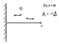
Figure 1: For a particle Q free to move in a semi-space, bounded by a rigid wall located at $x=0$, the operator $-i\partial/\partial x$ has the clear physical meaning of the particle momentum $x$-component even if it is not selfadjoint (cf. von Neumann[34], and Ref.[6]): See the text.

At this point, let us emphasize that our previously assumed boundary condition $E\neq 0$ can be dispensed with, by having recourse[2, 6] to the bi-linear hermitian operator

$$\hat{t}=\displaystyle\frac{-i\hbar}{2}\displaystyle\frac{\stackrel{{\scriptstyle\leftrightarrow}}{{\partial}}}{\partial E}$$ (10)

where the meaning of the sign $\leftrightarrow$ is clear from the accompanying definition

$$(f,\,\hat{t}\,g)=\Bigl{(}f,\>-\displaystyle\frac{ih}{2}\displaystyle\frac{\partial}{\partial E}\,g\Bigr{)}+\Bigl{(}-\displaystyle\frac{ih}{2}\,\displaystyle\frac{\partial}{\partial E}\,f,\;g\Bigr{)}\,.$$

By adopting this expression for the time operator, the algebraic sum of the two terms in the r.h.s. of the last relation results to be automatically zero at point $E=0$. This question will be exploited below, in Sect.3 (when dealing with the more general case of the four-position operator). Incidentally, such an “elimination”[6, 2] of point $E=0$ is not only simpler, but also more physical, than other kinds of elimination obtained much later in papers like [26].

In connection with the last quotation, leu us for briefly comment on the so-called positive-operator-value-measure (POVM) approach, often used or discussed in the second set of papers on time in quantum physics mentioned in our Introduction. Actually, an analogous procedure had been proposed, since the sixties[48], in some approaches to the quantum theory of measurements. Afterwards, and much later, the POVM approach has been applied, in a simplified and shortened form, to the time-operator problem in the case of one-dimensional free motion: for instance, in Refs.[10, 12, 15, 22–29] and especially in [26]. These papers stated that a generalized decomposition of unity (or “POV measure”) could be obtained from selfadjoint extensions of the time operator inside an extended Hilbert space (for instance, adding the negative values of the energy, too), by exploiting the Naimark dilation-theorem[35]: But such a program has been realized till now only in the simple cases of one-dimensional particle free motion.

By contrast, our approach is based on a different Naimark’s theorem[30], which, as already mentioned above, allows a much more direct, simple and general –and at the same time non less rigorous– introduction of a quantum operator for Time.  More precisely, our approach is based on the so-called Carleman theorem[50], utilized in Ref.[30], about approximating a hermitian operator by suitable successions of “bounded” selfadjoint operators: That is, of selfadjoint operators whose spectral functions do weakly converge to the non-orthogonal spectral function of the considered hemitian operator.  And our approach is applicable to a large family of three-dimensional (3D) particle collisions, with all possible Hamiltonians. Actually, our approach was proposed in the early Refs.[2–7] and in the first one of Ref.[18], and applied therein for the time analysis of quantum collisions, nuclear reactions and tunnelling processes.

2.2 On the momentum representation of the Time operator

In the continuous spectrum case, instead of the $E$-representation, with $0<E<+\infty$, in eqs.(1)–(4) one can also use the $k$-representation[9], with the advantage that $-\infty<k<+\infty$:

$$\Psi\,(x,t)=\displaystyle\int\limits_{-\infty}^{+\infty}g(k)\,\varphi(x,k)\,\exp(-iEt/\hbar)\>dk$$ (11)

with $E=\hbar^{2}k^{2}/\,2\mu$, and $k\neq 0$.

For the extension of the momentum representation to the case of $\langle t^{n}\rangle$, with $n>1$, we confine ourselves here to refer the reader to the papers [20, 49].

2.3 An alternative weight for time averages (in the cases of particle dwelling inside a certain spatial region)

We recall that the weight (2) [as well as its modifications (3)] has the meaning of a probability for the considered particle to pass through point $x$ during the time interval ($t$, $t+dt$). Let us follow the procedure presented in Refs.[18-21], and refs. therein, and analyze the consequences of the equality

$$\int\limits_{-\infty}^{+\infty}j\,(x,t)\>dt=\displaystyle\int\limits_{-\infty}^{+\infty}\bigl{|}\,\Psi(x,t)\bigr{|}^{2}\>dx$$ (12)

obtained from the 1D continuity equation. One can easily realize that a second, alternative weight can be adopted:

$$d\,P(x,t)\equiv Z\,(x,t)\>dx=\displaystyle\frac{\bigl{|}\Psi(x,t)\bigr{|}^{2}\>dx}{\displaystyle\int\limits_{-\infty}^{+\infty}\bigl{|}\,\Psi(x,t)\bigr{|}^{2}\>dx}$$ (13)

which possesses the meaning of probability for the particle to be located (or to sojourn, i.e., to dwell) inside the infinitesimal space region ($x$, $x+dx$) at the instant $t$, independently of its motion properties. Then, the quantity

$$P(x_{1},x_{2},t)=\displaystyle\frac{\displaystyle\int\limits_{x_{1}}^{x_{2}}\bigl{|}\Psi(x,t)\bigr{|}^{2}\>dx}{\displaystyle\int\limits_{-\infty}^{+\infty}\bigl{|}\,\Psi(x,t)\bigr{|}^{2}\>dx}$$ (14)

will have the meaning of probability for the particle to dwell inside the spatial interval ($x_{1}$, $x_{2}$) at the instant $t$.

As it is known (see, for instance, Refs.[18, 19, 20] and refs. therein), the mean dwell time can be written in the two equivalent forms:

$$\langle\tau(x_{i},x_{f})\rangle=\displaystyle\frac{\displaystyle\int\limits_{-\infty}^{+\infty}dt\ \displaystyle\int\limits_{x_{i}}^{x_{f}}|\Psi(x,t)|^{2}\;dx}{\displaystyle\int\limits_{-\infty}^{+\infty}j_{\rm in}(x_{i},t)\;dt}$$ (15)

and

$$\langle\tau(x_{i},x_{f})\rangle=\displaystyle\frac{\displaystyle\int\limits_{-\infty}^{+\infty}t\,j(x_{f},t)\;dt-\displaystyle\int\limits_{-\infty}^{+\infty}t\,j(x_{i},t)\;dt}{\displaystyle\int\limits_{-\infty}^{+\infty}j_{\rm in}(x_{i},t)\;dt}\;,$$ (16)

where it has been taken account, in particular, of relation (12), which follows —as already said— from the continuity equation.

Thus, in correspondence with the two measures (2) and (13), when integrating over time one gets two different kinds of time distributions (mean values, variances,…), which refer to the particle traversal time in the case of measure (2), and to the particle dwelling in the case of measure (13). Some examples for 1D tunneling are contained in Refs.[18, 19, 20].

2.4 Time as a quantum-theoretical Observable in the case of Photons

As is known (see, for instance, Refs.[36, 19]), in first quantization the single-photon wave function can be probabilistically described in the 1D case by the wave-packet

$${\mbox{\boldmath$A$}}({\mbox{\boldmath$r$}},t)=\displaystyle\int\limits_{k_{0}}\displaystyle\frac{d^{3}k}{k_{0}}\;{\mbox{\boldmath$\chi$}}({\mbox{\boldmath$k$}})\>\varphi({\mbox{\boldmath$k$}},{\mbox{\boldmath$r$}})\>\exp(-ik_{0}t)\;,$$ (17)

where, as usual, ${\mbox{\boldmath$A$}}({\mbox{\boldmath$r$}},t)$ is the electromagnetic vector potential, while ${\mbox{\boldmath$r$}}=\{x,y,z\}$,  ${\mbox{\boldmath$k$}}=\{k_{x},k_{y},k_{z}\}$,  $k_{0}\equiv w/c=\varepsilon/\,\hbar c$, and $k\equiv|{\mbox{\boldmath$k$}}|=k_{0}$. The axis $x$ has been chosen as the propagation direction. Let us notice that ${\mbox{\boldmath$\chi$}}({\mbox{\boldmath$k$}})=\sum\limits_{i=y,z}\chi_{i}({\mbox{\boldmath$k$}})\,{\mbox{\boldmath$e$}}_{i}({\mbox{\boldmath$k$}})$,  with  ${\mbox{\boldmath$e$}}_{i}{\mbox{\boldmath$e$}}_{j}=\delta_{ij}$, and $x_{i},x_{j}=y,z$, while $\chi_{i}({\mbox{\boldmath$k$}})$ is the probability amplitude for the photon to have momentum $k$ and polarization ${\mbox{\boldmath$e$}}_{j}$ along $x_{j}$. Moreover, it is $\varphi({\mbox{\boldmath$k$}},{\mbox{\boldmath$r$}})=\exp(ik_{x}x)$ in the case of plane waves, while $\varphi({\mbox{\boldmath$k$}},{\mbox{\boldmath$r$}})$ is a linear combination of evanescent (decreasing) and anti-evanescent (increasing) waves in the case of “photon barriers” (i.e., band-gap filters, or even undersized segments of waveguides for microwaves, or frustrated total-internal-reflection regions for light, and so on). Although it is not easy to localize a photon in the direction of its polarization[36], nevertheless for 1D propagations it is possible to use the space-time probabilistic interpretation of eq.(17), and define the quantity

$$\begin{array}[]{cc}\rho_{\rm em}(x,t)\>dx=\displaystyle\frac{S_{0}\>dx}{\int S_{0}\>dx},&S_{0}=\displaystyle\int\displaystyle\int s_{0}\>dy\,dz\end{array}$$ (18)

($s_{0}=[{\mbox{\boldmath$E$}}^{*}\cdot{\mbox{\boldmath$E$}}+{\mbox{\boldmath$H$}}^{*}\cdot{\mbox{\boldmath$H$}}]/\,4\pi$ being the energy density, with the electromagnetic field ${\mbox{\boldmath$H$}}={\rm rot}\,{\mbox{\boldmath$A$}}$,  and  $\mbox{\boldmath$E$}=-1/c\;\partial{\mbox{\boldmath$A$}}/\partial t$), which represents the probability density of a photon to be found (localized) in the spatial interval ($x$, $x+dx$) along the $x$-axis at the instant $t$;  and the quantity

$$\begin{array}[]{cc}j_{\rm em}(x,t)\>dt=\displaystyle\frac{S_{x}\>dt}{\int S_{x}(x,t)\>dt},&S_{x}(x,t)=\displaystyle\int\displaystyle\int s_{x}\>dy\,dz\end{array}$$ (19)

($s_{x}=c\;\Re[{\mbox{\boldmath$E$}}^{*}\wedge{\mbox{\boldmath$H$}}]_{x}\,/\>8\pi$ being the energy flux density), which represents the flux probability density of a photon to pass through point $x$ in the time interval ($t$, $t+dt$): in full analogy with the probabilistic quantities for non-relativistic particles. The justification and convenience of such definitions is self-evident, when the wave-packet group velocity coincides with the velocity of the energy transport;  in particular:  (i) the wave-packet (17) is quite similar to wave-packets for non-relativistic particles,  and  (ii) in analogy with conventional non-relativistic quantum mechanics, one can define the “mean time instant” for a photon (i.e., an electromagnetic wave-packet) to pass through point $x$, as follows

$$\langle t(x)\rangle=\displaystyle\int\limits_{-\infty}^{+\infty}t\,J_{{\rm em},\,x}\;dt=\displaystyle\frac{\displaystyle\int\limits_{-\infty}^{+\infty}t\,S_{x}(x,t)\;dt}{\displaystyle\int\limits_{-\infty}^{+\infty}S_{x}(x,t)\;dt}\;.$$

As a consequence [in the same way as in the case of equations (1)–(2)], the form (1) for the time operator in the energy representation is valid also for photons, with the same boundary conditions adopted in the case of particles, that is, with $\chi_{i}\,(0)=\chi_{i}\,(\infty)$ and with $E=\hbar\,c\,k_{0}$.

The energy density $s_{0}$ and energy flux density $s_{x}$ satisfy the relevant continuity equation

$$\frac{\partial s_{0}}{\partial t}+\displaystyle\frac{\partial s_{x}}{\partial x}=0$$ (20)

which is Lorentz-invariant for 1D spatial propagation[19, 20] processes.

2.5 Introducing the analogue of the “Hamiltonian” for the case of the Time operator: A new hamiltonian approach

In non-relativistic quantum theory, the Energy operator acquires (cf., e.g., Refs.[8, 20]) the two forms:  (i)  $i\hbar\,\displaystyle\frac{\partial}{\partial t}$ in the $t$-representation, and  (ii)  $\hat{H}\,(\hat{p}_{x},\hat{x},\ldots)$ in the hamiltonianian formalism. The “duality” of these two forms can be easily inferred from the Schröedinger equation itself,  $\hat{H}\Psi=i\hbar\displaystyle\frac{\partial\Psi}{\partial t}$. One can introduce in quantum mechanics a similar duality for the case of Time: Besides the general form (1) for the Time operator in the energy representation, which is valid for any physical systems in the region of continuous energy spectra, one can express the time operator also in a “hamiltonian form”, i.e., in terms of the coordinate and momentum operators, by having recourse to their commutation relations.  Thus, by the replacements

$$\begin{array}[]{c}\vspace{3mm}\hat{E}\to\hat{H}\,(\hat{p}_{x},\hat{x},\ldots),\\ \hat{t}\to\hat{T}\,(\hat{p}_{x},\hat{x},\ldots),\end{array}$$ (21)

and on using the commutation relation [similar to eq.(3)]

$$[\hat{H},\,\hat{T}]=i\hbar\;,$$ (22)

one can obtain[37], given a specific ordinary Hamiltonian, the corresponding explicit expression for $\hat{T}\,(\hat{p}_{x},\hat{x},\ldots)$.

Indeed, this procedure can be adopted for any physical system with a known Hamiltonian $\hat{H}\,(\hat{p}_{x},\hat{x},\ldots)$, and we are going to see a concrete example. By going on from the coordinate to the momentum representation, one realizes that the formal expressions of both the hamiltonian-type operators $\hat{H}\,(\hat{p}_{x},\hat{x},\ldots)$ and $\hat{T}\,(\hat{p}_{x},\hat{x},\ldots)$ do not change, except for an obvious change of sign in the case of operator $\hat{T}\,(\hat{p}_{x},\hat{x},\ldots)$.

As an explicit example, let us address the simple case of a free particle whose Hamiltonian is

$$\hat{H}=\left\{\begin{array}[]{ccll}\hat{p}_{x}^{2}/\,2\mu,&\hat{p}_{x}=-i\hbar\displaystyle\frac{\partial}{\partial x}\,,&\mbox{ \ \ \ \ in the coordinate representation}&\mbox{(a)}\\ p_{x}^{2}/\,2\mu\,.&&\mbox{ \ \ \ \ in the momentum representation}&\mbox{(a)}\end{array}\right.$$ (23)

Correspondingly, the Hamilton-type time operator, in its symmetrized form, will write

$$\hat{T}=\left\{\begin{array}[]{clll}\vspace{2mm}\displaystyle\frac{\mu}{2}\,\Bigl{(}\hat{p}_{x}^{-1}x+x\hat{p}_{x}^{-1}+i\hbar\,;\ \hat{p}_{x}^{-2}\Bigr{)},&{\rm in\ the\ coordinate\ representation}&\mbox{(a)}\\ -\displaystyle\frac{\mu}{2}\,\Bigl{(}p_{x}^{-1}\hat{x}+\hat{x}p_{x}^{-1}+i\hbar/p_{x}^{2}\Bigr{)},&{\rm in\ the\ momentum\ representation}&\mbox{(b)}\end{array}\right.$$ (24)

where

$$\begin{array}[]{cc}\hat{p}_{x}^{-1}=\displaystyle\frac{i}{\hbar}\int dx\ldots,&\hskip 19.91692pt\hat{x}=i\hbar\displaystyle\frac{\partial}{\partial p_{x}}\;.\end{array}$$

Incidentally, operator (24b) is equivalent to $-i\hbar\,\frac{\partial}{\partial E}$, since $E=p_{x}^{2}/\,2\mu$; and therefore it is also a (maximal) hermitian operator. Indeed, by applying the operator $\hat{T}\,(\hat{p}_{x},\hat{x},\ldots)$, for instance, to a plane-wave of the type $\exp(ikx)$, we obtain the same result in both the coordinate and the momentum representations:

$$\hat{T}\;\exp(ikx)=\displaystyle\frac{x}{v}\>\exp(ikx)$$ (25)

quantity ${x}/{v}$ being the free-motion time (for a particle with velocity $v$ ) for traveling the distance $x$.

On the basis of what precedes, it is possible to show that the wave function $\Psi(x,t)$ of a quantum system satisfies the two (dual) equations

$$\begin{array}[]{ccc}\hat{H}\,\Psi=i\hbar\displaystyle\frac{\partial\Psi}{\partial t}&\mbox{and}&\hat{T}\,\Psi=t\,\Psi\,.\end{array}$$ (26)

In the energy representation, and in the stationary case, we obtain again two (dual) equations

$$\begin{array}[]{ccc}\hat{H}\,\varphi_{t}=\varepsilon\,\varphi_{t}&\mbox{and}&\hat{T}\,\varphi_{t}=-i\hbar\displaystyle\frac{\partial\varphi_{t}}{\partial\varepsilon}\;,\end{array}$$ (27)

quantity $\varphi_{t}$ being the Fourier-transform of $\Psi$:

$$\varphi_{t}=\displaystyle\frac{1}{2\pi\hbar}\displaystyle\int\limits_{-\infty}^{+\infty}\Psi(x,t)\>e^{i\varepsilon t/\hbar}\;dt\,.$$ (28)

It might be interesting to apply the two pairs of the last dual equations also for investigating tunnelling processes through the quantum gravitational barrier, which appears during inflation, or at the beginning of the big-bang expansion, whenever a quasi-linear Schroedinger-type equation does approximately show up.

2.6 Time as an Observable (and the Time-Energy uncertainty relation), for quantum-mechanical systems with discrete energy spectra

For describing the time evolution of non-relativistic quantum systems endowed with a purely discrete (or a continuous and discrete) spectrum, let us now introduce wave-packets of the form[8, 20, 49]:

$$\psi\,(x,t)=\sum\limits_{n=0}g_{n}\,\varphi_{n}(x)\,\exp[-i(\varepsilon_{n}-\varepsilon_{0})t/\hbar]\;,$$ (29)

where $\varphi_{n}(x)$ are orthogonal and normalized bound states which satisfy the equation $\hat{H}\,\varphi_{n}(x)=\varepsilon_{n}\,\varphi_{n}(x)$, quantity $\hat{H}$ being the Hamiltonian of the system; while the coefficients $g_{n}$ are normalized: $\sum\limits_{n=0}|g_{n}|^{2}=1$. We omitted the non-significant phase factor $\exp(-i\varepsilon_{0}t/\hbar)$ of the fundamental state.

Let us first consider the systems whose energy levels are separated by intervals admitting a maximum common divisor $D$ (for ex., harmonic oscillator, particle in a rigid box, and spherical spinning top), so that the wave packet (29) is a periodic function of time possessing as period the Poincaré cycle time $T=2\pi\hbar/D$. For such systems it is possible[8, 20, 49] to construct a selfadjoint time operator with the form (in the time representation) of a saw-function of $t$, choosing $t=0$ as the initial time instant:

$$\hat{t}\;=\;t-T\sum_{n=0}^{\infty}\Theta(t-[2n+1]T/2)+T\sum_{n=0}^{\infty}\Theta(-t-[2n+1]T/2\;.$$ (30)

This periodic function for the time operator is a linear (increasing) function of time $t$ within each Poincar cycle: see Fig.2.

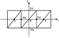
Figure 2: The periodic saw-tooth function for the time operator in the case of quantum mechanical systems with discrete energy spectra: Namely, for the case of eq.(30).

The commutation relations of the Energy and Time operators, now both selfajoint, acquires in the case of discrete energies and of a periodic Time operator the form

$$[\hat{E},\hat{t}]\;=\;i\hbar\left\{1-T\sum_{n=0}^{\infty}\delta(t-[2n+1]T)\right\}\,,$$ (31)

wherefrom the uncertainty relation follows in the new form

$$(\Delta E)^{2}\;(\Delta t)^{2}\;=\;\hbar^{2}\left[1-{{T|\psi(T/2+\gamma)|^{2}}\over{\int_{-T/2}^{T/2}|\psi(t)|^{2}dt}}\right]\;,$$ (32)

where it has been introduced a parameter $\gamma$, with $-T/2<\gamma<T/2$, in order to assure that the r.h.s. integral is single-valued[20, 49].

When $\Delta E\rightarrow 0$ (that is, when $|g_{n}|\rightarrow\delta_{nn^{\prime}})$, the r.h.s. of eq.32 tends to zero too, since $|\psi(t)|^{2}$ tends to a constant value. In such a case, the distribution of the time instants at which the wave-packet passes through point $x$ becomes flat within each Poincaré cycle. When, by contrast, $\Delta E>>D$ and  $|\psi(T+\gamma)|^{2}<<(\int_{-T/2}^{T/2}|\psi(t)|^{2}dt)/T$, the periodicity condition may become inessential whenever $\Delta t<<t$. In other words, our uncertainty relation (32) transforms into the ordinary uncertainty relation for systems with continuous spectra.

In more general cases, for excited states of nuclei, atoms and molecules, the energy-level intervals, for discrete and quasi-discrete (resonance) spectra, are not multiples of a maximum common divisor, and hence the Poincaré cycle is not well-defined for such systems.  Nevertheless, even for those systems one can introduce an approximate description (sometimes, with any desired degree of accuracy) in terms of Poincaré quasi-cycles and a quasi-periodical evolution; so that for sufficiently long time intervals the behavior of the wave-packets can be associated with a a periodical motion (oscillation), sometimes —e.g., for very narrow resonances— with any desired accuracy. For them, when choosing an approximate Poincaré-cycle time, one can include in one cycle as many quasi-cycles as it is necessary for the demanded accuracy. Then, with the chosen accuracy, a quasi-selfadjoint time operator can be introduced.

3 On four-position operators in quantum field theory, in terms of bilinear operators

In this Section we approach the relativistic case, taking into consideration —therefore— the space-time (four-dimensional) “position” operator, starting however with an analysis of the 3-dimensional (spatial) position operator in the simple relativistic case of the Klein-Gordon equation.

Actually, this analyzis will lead us to tackle already with non-hermitian operators.  Moreover, while performing it, we shall meet the opportunity of introducing bilinear operators, which will be used even more in the next case of the full 4-position operator.

Let us recall that in Sect.2.1 we mentioned that the boundary condition $E\neq 0$, therein imposed to guarantee (maximal) hermitity of the time operator, can be dispensed with just by having recourse to bilinear forms.  Namely, by considering the bilinear hermitian operator[6, 41]  $\hat{t}=(-i\hbar\;{\stackrel{{\scriptstyle\leftrightarrow}}{{\partial}}}/{\partial E})/2$,  where the sign $\leftrightarrow$ is defined through the accompanying equality  $(f,\,\hat{t}\,g)=\Bigl{(}f,\>-\frac{ih}{2}\frac{\partial}{\partial E}\,g\Bigr{)}+\Bigl{(}-\frac{ih}{2}\,\frac{\partial}{\partial E}\,f,\;g\Bigr{)}$.

3.1 The Klein-Gordon case: Three-position operators

The standard position operators, being hermitian and moreover selfadjoint, are known to possess real eigenvalues: i.e., they yield a point-like localization. J.M.Jauch showed, however, that a point-like localization would be in contrast with “unimodularity”. In the relativistic case, moreover, phenomena so as the pair production forbid a localization with precision better than one Compton wave-length. The eigenvalues of a realistic position operator ${\hat{\mbox{\boldmath$z$}}}$ are therefore expected to represent space regions, rather than points. This can be obtained only by having recourse to non-hermitian (and therefore non-selfadjoint) position operators ${\hat{\mbox{\boldmath$z$}}}$ (a priori, one can have recourse either to non-normal operators with commuting components, or to normal operators with non-commuting components). Following, e.g., the ideas in Ref.[38], we are going to show that the mean values of the hermitian (selfadjoint) part of ${\hat{\mbox{\boldmath$z$}}}$ will yield a mean (point-like) position[39], while the mean values of the anti-hermitian (anti-selfadjoint) part of ${\hat{\mbox{\boldmath$z$}}}$ will yield the sizes of the localization region[2].

Let us consider, e.g., the case of relativistic spin-zero particles, in natural units and with metric $(+\,-\,-\,-)$. The position operator $i\,\nabla_{\mbox{\boldmath$p$}}$, is known to be actually non-hermitian, and may be in itself a good candidate for an extended-type position operator. To show this, we want to split[38] it into its hermitian and anti-hermitian (or skew-hermitian) parts.

Consider, then, a vector space $V$ of complex differentiable functions on a 3-dimensional phase-space[41] equipped with an inner product defined by

$$(\Psi,\,\Phi)=\displaystyle\int\displaystyle\frac{d^{3}{\mbox{\boldmath$p$}}}{p_{0}}\;\Psi^{*}({\mbox{\boldmath$p$}})\,\Phi(p)$$ (33)

quantity $p_{0}$ being $\sqrt{{\mbox{\boldmath$p$}^{2}}+m_{0}^{2}}$. Let the functions in $V$ satisfy moreover the condition

$$\lim\limits_{R\to\infty}\displaystyle\int\limits_{S_{R}}\displaystyle\frac{dS}{p_{0}}\;\Psi^{*}(p)\,\Phi(p)=0$$ (34)

where the integral is taken over the surface of a sphere of radius $R$.  If $U:V\to V$ is a differential operator of degree one, condition (34) allows a definition of the transpose $U^{T}$ by

$$\begin{array}[]{ccc}(U^{T}\Psi,\,\Phi)=(\Psi,\,U\,\Phi)&\mbox{for all }\Psi,\,\Phi\in V\;,\end{array}$$ (35)

where $U$ is changed into $U^{T}$, or vice-versa, by means of integration by parts.

This allows, further, to introduce a dual representation[41] ($U_{1}$, $U_{2}$) of a single operator $U_{1}^{T}+U_{2}$ by

$$(U_{1}\Psi,\,\Phi)+(\Psi,\,U_{2}\Phi)=(\Psi,\,(U_{1}^{T}+U_{2})\,\Phi).$$ (36)

With such a dual representation, it is easy to split any operator into its hermitian and anti-hermitian parts

$$(\Psi,\,U\Phi)=\displaystyle\frac{1}{2}\,\Bigl{(}(\Psi,\,U\Phi)+(U^{*}\Psi,\,\Phi)\Bigr{)}+\displaystyle\frac{1}{2}\,\Bigl{(}(\Psi,\,U\Phi)-(U^{*}\Psi,\,\Phi)\Bigr{)}.$$ (37)

Here the pair

$$\frac{1}{2}\,(U^{*},\,U)\equiv\,\stackrel{{\scriptstyle\leftrightarrow}}{{U}}_{h}\;,$$ (38)

corresponding to $(1/2)\,(U+U^{*T})$, represents the hermitian part, while

$$\frac{1}{2}(-U^{*},\,U)\equiv\,\stackrel{{\scriptstyle\leftrightarrow}}{{U}}_{a}$$ (39)

represents the anti-hermitian part.

Let us apply what precedes to the case of the Klein-Gordon position-operator $\hat{z}=i\,\nabla_{p}$. When

$$U=i\,\displaystyle\frac{\partial}{\partial p_{j}}$$ (40)

we have[2]

$$\begin{array}[]{cl}\vspace{2mm}\displaystyle\frac{1}{2}\,(U^{*},\,U)=\displaystyle\frac{1}{2}\,\biggl{(}-i\,\displaystyle\frac{\partial}{\partial p_{j}},\,i\,\displaystyle\frac{\partial}{\partial p_{j}}\biggr{)}\equiv\,\displaystyle\frac{i}{2}\,\displaystyle\frac{\stackrel{{\scriptstyle\leftrightarrow}}{{\partial}}}{\partial p_{j}},&(a)\\ \displaystyle\frac{1}{2}\,(-U^{*},\,U)=\displaystyle\frac{1}{2}\,\biggl{(}i\,\displaystyle\frac{\partial}{\partial p_{j}},\,i\,\displaystyle\frac{\partial}{\partial p_{j}}\biggr{)}\equiv\,\displaystyle\frac{i}{2}\,\displaystyle\frac{\stackrel{{\scriptstyle\leftrightarrow}}{{\partial}}_{+}}{\partial p_{j}}.&(b)\end{array}$$ (41)

And the corresponding single operators turn out to be

$$\begin{array}[]{ll}\vspace{2mm}\displaystyle\frac{1}{2}\,(U+U^{*T})=i\,\displaystyle\frac{\partial}{\partial p_{j}}-\displaystyle\frac{i}{2}\,\displaystyle\frac{p_{j}}{p^{2}+m_{0}^{2}},&(a)\\ \displaystyle\frac{1}{2}\,(U-U^{*T})=\displaystyle\frac{i}{2}\,\displaystyle\frac{p_{j}}{p^{2}+m_{0}^{2}}\;.&(b)\end{array}$$ (42)

It is noteworthy[2] that, as we are going to see, operator (42a) is nothing but the usual Newton-Wigner operator, while (42b) can be interpreted[38, 2, 24] as yielding the sizes of the localization-region (an ellipsoid) via its average values over the considered wave-packet.

Let us underline that the previous formalism justifies from the mathematical point of view the treatment presented in papers like [38, 39].  We can split[2] the operator $\hat{z}$ into two bilinear parts, as follows:

$$\hat{z}=i\,\nabla_{p}=\displaystyle\frac{i}{2}\,\stackrel{{\scriptstyle\leftrightarrow}}{{\nabla}}_{p}+\displaystyle\frac{i}{2}\,\stackrel{{\scriptstyle\leftrightarrow}}{{\nabla}}_{p}^{(+)}$$ (43)

where  $\Psi^{*}\stackrel{{\scriptstyle\leftrightarrow}}{{\nabla}}_{p}\Phi\equiv\,\Psi^{*}\nabla_{p}\Phi-\Phi\nabla_{p}\Psi^{*}$  and  $\Psi^{*}\stackrel{{\scriptstyle\leftrightarrow}}{{\nabla}}_{p}^{(+)}\Phi\equiv\,\Psi^{*}\nabla_{p}\Phi+\Phi\nabla_{p}\Psi^{*}\,,$ and where we always referred to a suitable[38, 39, 6, 41] space of wave packets. Its hermitian part[38, 39]

$$\hat{x}=\displaystyle\frac{i}{2}\,\stackrel{{\scriptstyle\leftrightarrow}}{{\nabla}}_{p}\;,$$ (44)

which was expected to yield an (ordinary) point-like localization, has been derived also by writing explicitly

$$(\Psi,\,\hat{x}\,\Phi)=i\,\displaystyle\int\displaystyle\frac{d^{3}p}{p_{0}}\;\Psi^{*}(p)\,\nabla_{p}\,\Phi(p)$$ (45)

and imposing hermiticity, i.e., imposing the reality of the diagonal elements. The calculations yield

$$\Re\,\bigl{(}\Phi,\,\hat{x}\,\Phi\bigr{)}=i\,\displaystyle\int\displaystyle\frac{d^{3}p}{p_{0}}\;\Phi^{*}(p)\,\stackrel{{\scriptstyle\leftrightarrow}}{{\nabla}}_{p}\,\Phi(p)\;,$$ (46)

suggesting to adopt just the Lorentz-invariant quantity (44) as a bilinear hermitian position operator.  Then, on integrating by parts (and due to the vanishing of the surface integral), we verify that eq.(44) is equivalent to the ordinary Newton-Wigner operator:

$$\hat{x}_{h}\equiv\,\displaystyle\frac{i}{2}\,\stackrel{{\scriptstyle\leftrightarrow}}{{\nabla}}_{p}\>\equiv\,i\,\nabla_{p}-\displaystyle\frac{i}{2}\,\displaystyle\frac{{\mbox{\boldmath$p$}}}{p^{2}+m^{2}}\;\equiv{\rm N-W}\,.$$ (47)

We are left with the (bilinear) anti-hermitian part

$$\hat{y}=\displaystyle\frac{i}{2}\,\stackrel{{\scriptstyle\leftrightarrow}}{{\nabla}}_{p}^{(+)}$$ (48)

whose average values over the considered state (wave-packet) can be regarded as yielding[38, 39, 6, 41]the sizes of an ellipsoidal localization-region.

After the digression associated with eqs.(43)–(48), let us go back to the present formalism, as expressed by eqs.(33)–(42).

In general, the extended-type position operator $\hat{z}$ will yeld

$$\langle\Psi|\,\hat{z}\,|\Psi\rangle=(\alpha+\Delta\alpha)+i\,(\beta+\Delta\beta)\;,$$ (49)

where $\Delta\alpha$ and $\Delta\beta$ are the mean-errors encountered when measuring the point-like position and the sizes of the localization region, respectively. It is interesting to evaluate the commutators ($i,j=1,2,3$):

$$\biggl{(}\displaystyle\frac{i}{2}\,\displaystyle\frac{\stackrel{{\scriptstyle\leftrightarrow}}{{\partial}}}{\partial p_{i}},\,\displaystyle\frac{i}{2}\,\displaystyle\frac{\stackrel{{\scriptstyle\leftrightarrow}}{{\partial}}_{(+)}}{\partial p_{j}}\biggr{)}=\displaystyle\frac{i}{2\,p_{0}^{2}}\,\biggl{(}\delta_{ij}-\displaystyle\frac{2\,p_{i}p_{j}}{p_{0}^{2}}\biggr{)}\,,$$ (50)

wherefrom the noticeable “uncertainty correlations” follow:

$$\Delta\alpha_{i}\ \Delta\beta_{j}\geq\displaystyle\frac{1}{4}\;\biggl{|}\biggl{\langle}\displaystyle\frac{1}{p_{0}^{2}}\;\biggl{(}\delta_{ij}-\displaystyle\frac{2\,p_{i}p_{j}}{p_{0}^{2}}\biggr{)}\biggr{\rangle}\biggr{|}\,.$$ (51)

3.2 Four-position operators

It is tempting to propose as four-position operator the quantity $\hat{z}^{\mu}=\hat{x}^{\mu}+i\,\hat{y}^{\mu}$, whose hermitian (Lorentz-covariant) part can be written

$$\hat{x}^{\mu}=-\,\displaystyle\frac{i}{2}\,\displaystyle\frac{\stackrel{{\scriptstyle\leftrightarrow}}{{\partial}}}{\partial p_{\mu}}\;,$$ (52)

to be associated with its corresponding “operator” in four-momentum space

$$\hat{p}_{h}^{\mu}=+\>\displaystyle\frac{i}{2}\,\displaystyle\frac{\stackrel{{\scriptstyle\leftrightarrow}}{{\partial}}}{\partial x_{\mu}}\;.$$ (53)

Let us recall the proportionality between the 4-momentum operator and the 4-current density operator in the chronotopical space, and then underline the canonical correspondence (in the 4-position and 4-momentum spaces, respectively) between the “operators” (cf. the previous subsection):

$$\begin{array}[]{ll}\vspace{2mm}m_{0}\,\hat{\rho}\,\equiv\,\hat{p}_{0}=\displaystyle\frac{i}{2}\,\displaystyle\frac{\stackrel{{\scriptstyle\leftrightarrow}}{{\partial}}}{\partial t}&(a)\\ m_{0}\,\hat{{\mbox{\boldmath$j$}}}\,\equiv\,\hat{{\mbox{\boldmath$p$}}}=-\displaystyle\frac{i}{2}\,\displaystyle\frac{\stackrel{{\scriptstyle\leftrightarrow}}{{\partial}}}{\partial{\mbox{\boldmath$r$}}}\;,&(b)\end{array}$$ (54)

and the operators

$$\begin{array}[]{ll}\vspace{2mm}\hat{t}\,\equiv\,-\displaystyle\frac{i}{2}\,\displaystyle\frac{\stackrel{{\scriptstyle\leftrightarrow}}{{\partial}}}{\partial p_{0}}&(a)\\ \hat{{\mbox{\boldmath$x$}}}\,\equiv\,\displaystyle\frac{i}{2}\,\displaystyle\frac{\stackrel{{\scriptstyle\leftrightarrow}}{{\partial}}}{\partial{\mbox{\boldmath$p$}}}\;,&(b)\end{array}$$ (55)

where the four-position “operator” (55) can be considered as a 4-current density operator in the energy-impulse space.  Analogous considerations can be carried on for the anti-hermitial parts (see the last one of Refs.[2]).

Finally, by recalling the properties of the time operator as a maximal hermitian operator in the non-relativistic case (Sec.2.1), one can see that the relativistic time operator (55a) (for the Klein-Gordon case) is also a selfadjoint bilinear operator for the case of continuous energy spectra, and a (maximal) hermitian linear operator for free particles [due to the presence of the lower limit zero for the kinetic energy, or $m_{0}$ for the total energy].

4 Unstable states and non-hermitian Hamiltonians

4.1 Introduction

This whole Section is based on work performed in collaboration with A.Agodi, M.Baldo, and A.Pennisi di Floristella.[40]

In quantum mechanics the “Resonance” peaks are generally described as corresponding to unstable states (remember, e.g., Schwinger’s approach[42]). The present attempt proceeds as follows: (i) singling out one state $|\varphi\rangle$ in the state space; (ii) finding out the effect of the (internal, virtual) state $|\varphi\rangle$ on the transition-amplitude; (iii) finding, in particular, the necessary conditions for $|\varphi\rangle$ to be connected with a Resonance in the cross-section. In this way one can associate the “resonant state” with the eigenvectors of a non-hermitian Hamiltonian (or rather, for simplicity, of a “quasi hermitian” Hamiltonian), such eigenvectors decaying correctly in time. We shall adopt the formalism introduced by Akhiezer and Glazman[32], by Lifshitz, by Galitsky and Migdal[43], and by Agodi et al.[44].

Chosen a state $|\,\varphi\rangle$, let us define the projectors

$$\begin{array}[]{ll}P\equiv|\,\varphi\rangle\;\langle\varphi|,&Q=1-P\;,\end{array}$$ (56)

where 1 is the identity operator.

4.2 Preliminary case: time-dependent description of potential scattering

Let us preliminarily consider the time-dependent description of potential scattering. Quantity $V$ be the potential operator. In the limiting case of plane-waves, the scattering amplitude writes

$$\begin{array}[]{ll}T({\mbox{\boldmath$k$}},{\mbox{\boldmath$k$}}^{\prime})=\langle{\mbox{\boldmath$k$}}^{\prime}|\,V\,|\,{\mbox{\boldmath$k$}}\rangle+\langle{\mbox{\boldmath$k$}}^{\prime}|\,V\,G(E^{+})\,V\,|\,{\mbox{\boldmath$k$}}\rangle\end{array}$$ (57)

with

$$\begin{array}[]{ll}G(E^{+})\equiv(E^{+}-H)^{-1},&E^{\pm}\equiv E\pm i\varepsilon\;.\end{array}$$ (58)

Chosen the exploring vector $|\,\varphi\rangle$ and using definition (56), we have

$$\begin{array}[]{ll}H=\stackrel{{\scriptstyle 0}}{{H}}+\stackrel{{\scriptstyle 1}}{{H}},\\ \stackrel{{\scriptstyle 0}}{{H}}=QHQ,&\stackrel{{\scriptstyle 1}}{{H}}=PHP+PHQ+QHP\;.\end{array}$$ (59)

By introducing the scattering states $|\stackrel{{\scriptstyle 0}}{{\varphi}}\rangle$ due to $\stackrel{{\scriptstyle 0}}{{H}}$

$$|\,\varphi^{\pm}_{{\mbox{\boldmath$k$}}}\rangle=\Biggl{\{}1+\displaystyle\frac{1}{E^{\pm}-\stackrel{{\scriptstyle 0}}{{H}}}\,\Bigl{(}\stackrel{{\scriptstyle 0}}{{H}}-E\Bigr{)}\Biggr{\}}\ |\,{\mbox{\boldmath$k$}}\rangle,$$ (60)

we obtain

$$\begin{array}[]{lcl}S({\mbox{\boldmath$k$}},{\mbox{\boldmath$k$}}^{\prime})&\equiv&\langle\varphi_{{\mbox{\boldmath$k$}}^{\prime}}^{(-)}|\,\varphi_{{\mbox{\boldmath$k$}}}^{(+)}\rangle=\langle\stackrel{{\scriptstyle 0}}{{\varphi_{{\mbox{\boldmath$k$}}^{\prime}}}}{}^{(-)}|\,\stackrel{{\scriptstyle 0}}{{\varphi_{{\mbox{\boldmath$k$}}}}}{}^{(+)}\rangle-2\pi\,\delta(E_{{\mbox{\boldmath$k$}}^{\prime}}-E_{{\mbox{\boldmath$k$}}})\\ &\times&\langle\stackrel{{\scriptstyle 0}}{{\varphi_{{\mbox{\boldmath$k$}}^{\prime}}}}{}^{(-)}|\>HP\,G(E^{+}_{{\mbox{\boldmath$k$}}})\,PH\>|\stackrel{{\scriptstyle 0}}{{\varphi_{{\mbox{\boldmath$k$}}}}}{}^{(+)}\rangle\;,\end{array}$$ (61)

where the first addendum in the r.h.s. of eq.(61) (let us call it $A$) is the contribution coming from processes developing entirely in the subspace onto which $Q$ projects, whilst the second addendum ($B$) is contributed by processes going through the exploring state $|\,\varphi\rangle$ onto which $P$ projects. In other words, the processes with $|\,\varphi\rangle$ as intermediate state correspond to the term

$$\begin{array}[]{ll}\Bigl{(}2\pi\,\delta(E_{{\mbox{\boldmath$k$}}^{\prime}}-E_{{\mbox{\boldmath$k$}}})\Bigr{)}^{-1}\ B=-2\pi i\;\displaystyle\frac{\langle\stackrel{{\scriptstyle 0}}{{\varphi}}{}_{{\mbox{\boldmath$k$}}^{\prime}}^{(-)}|\,H\,|\,\varphi\rangle\;\langle\varphi|\,H\,|\stackrel{{\scriptstyle 0}}{{\varphi}}{}_{{\mbox{\boldmath$k$}}}^{(+)}\rangle}{E_{{\mbox{\boldmath$k$}}}^{+}-\langle\varphi|\,H\,|\,\varphi\rangle-\langle\varphi|\,W^{\varphi}(E_{{\mbox{\boldmath$k$}}}^{+})\,|\,\varphi\rangle},\\ W^{\varphi}(z)=PHQ\>\displaystyle\frac{1}{z-QHQ}\>QHP\;.\end{array}$$ (62)

Our problem is: under what conditions one (or more) Resonances are actually associated with the chosen $|\,\varphi\rangle$? Let us notice in particular that, if $E_{\varphi}\equiv\langle\varphi|\,H\,|\,\varphi\rangle-\Re\,\langle\varphi|\,W^{\varphi}(E^{+})\,|\,\varphi\rangle$ and $\Gamma_{\varphi}\equiv\Im\,\langle\varphi|\,W^{\varphi}(E^{+})\,|\,\varphi\rangle$ are smooth functions of $E$, then $B$ gets just the “Breit and Wigner” form:

$$B=-2\pi i\;\displaystyle\frac{\langle\stackrel{{\scriptstyle 0}}{{\varphi}}{}_{{\mbox{\boldmath$k$}}^{\prime}}^{(-)}|\,HPH\,|\stackrel{{\scriptstyle 0}}{{\varphi}}{}_{{\mbox{\boldmath$k$}}}^{(+)}\rangle}{E-E_{\varphi}+i\,\Gamma_{\varphi}}\;.$$ (63)

4.3 Case of central potential and spin-free particles

Let us choose the angular-momentum representation. If $|\,\varphi\rangle$ is assumed to be in particular invariant under O(3), then both terms in which $S$ was split are diagonal. If $\stackrel{{\scriptstyle 0}}{{\delta_{2}}}$ are the phase-shifts due to $QHQ$ and $\mu$ is the reduced mass, then

$$S_{2}({\mbox{\boldmath$k$}})\equiv\exp(2i\,\delta_{2}({{\mbox{\boldmath$k$}}}))=F_{2}({\mbox{\boldmath$k$}})\;\exp(2i\stackrel{{\scriptstyle 0}}{{\delta_{2}}}({\mbox{\boldmath$k$}}))\;,$$ (64)

with

$$F_{2}({\mbox{\boldmath$k$}})\equiv 1-\displaystyle\frac{2\pi i\mu}{2{\mbox{\boldmath$k$}}}\;\displaystyle\frac{\Bigl{|}\langle\varphi|\,H\,|\stackrel{{\scriptstyle 0}}{{\varphi}}{}^{(+)}_{klm}\rangle\Bigr{|}^{2}}{E^{+}-\langle\varphi|\,H\,|\,\varphi\rangle-\langle\varphi|\,W^{\varphi}(E_{{\mbox{\boldmath$k$}}}^{+})\,|\,\varphi\rangle}\;.$$ (65)

Let us observe that the phase-shift of $F_{2}({\mbox{\boldmath$k$}})$ crosses the value $\frac{1}{2}\,\pi$ (with positive slope) when

$$F_{2}({\mbox{\boldmath$k$}})=-1.$$ (66)

The condition for a Resonance to appear are particularly transparent for $l=0$:

$$F_{0}({\mbox{\boldmath$k$}})=\displaystyle\frac{E-E_{\varphi}-i\,\lambda_{0}({\mbox{\boldmath$k$}})}{E-E_{\varphi}+i\,\lambda_{0}({\mbox{\boldmath$k$}})}\;,$$ (67)

when

$$\lambda_{0}({\mbox{\boldmath$k$}})\equiv-\Im\,\langle\varphi|\,W^{\varphi}(E_{{\mbox{\boldmath$k$}}}^{+})\,|\,\varphi\rangle=\Bigl{|}\langle\varphi|\,H\,|\stackrel{{\scriptstyle 0}}{{\varphi}}{}_{k00}^{(+)}\rangle\Bigr{|}^{2}$$ (68)

is positive-definite. Namely, the condition $F_{0}({\mbox{\boldmath$k$}})=-1$ yields

$$|1-S_{0}({\mbox{\boldmath$k$}})|^{2}=4\,\cos^{2}\stackrel{{\scriptstyle 0}}{{\delta}}_{0}\;,$$ (69)

with the supplementary conditions $\lambda_{0}({\mbox{\boldmath$k$}})\neq 0$ and $\cos\stackrel{{\scriptstyle 0}}{{\delta}}_{0}\neq 0$. When $\cos\stackrel{{\scriptstyle 0}}{{\delta}}_{0}=1$ the scattering due to $QHQ$ is negligible, i.e., the scattering proceeds entirely via the intermediate formation of the (quasi-bound) state $|\,\varphi\rangle$; and the possible resonant effects are really related to $|\,\varphi\rangle$. Of course, $\cos\stackrel{{\scriptstyle 0}}{{\delta}}_{0}=1$ when, at the resonance

$$\begin{array}[]{ll}E=E_{\varphi},&F({\mbox{\boldmath$k$}})=-1\;,,\end{array}$$ (70)

it is $|\stackrel{{\scriptstyle 0}}{{\varphi}}{}_{klm}^{(\pm)}\rangle=|\,lm\rangle$.

Notice that with every fixed $|\,\varphi\rangle$ a series of Resonances (also for different value of $l$) may be a priori associated, if they are not destroyed by the $\stackrel{{\scriptstyle 0}}{{\delta}}_{0}$ behavior.

4.4 Resonance definition

It is essential to recognize that the “resonance condition” $F_{l}({\mbox{\boldmath$k$}})=-1$ may be written [40]

$$1-\alpha\,({\mbox{\boldmath$k$}},l)\>\langle\varphi_{2}|\,G(E^{+})\,|\,\varphi_{2}\rangle=0\;,$$ (71)

with

$$\alpha\,({\mbox{\boldmath$k$}},l)=\displaystyle\frac{i\pi\mu}{2{\mbox{\boldmath$k$}}}\;\Bigl{|}\langle\varphi_{2}|\,H\,|\stackrel{{\scriptstyle 0}}{{\varphi}}{}^{(+)}_{klm}\rangle\Bigr{|}^{2}.$$ (72)

Let us now study the more general equation

$$1-\lambda\;\langle\varphi_{2}|\,G(z)\,|\,\varphi_{2}\rangle=0\;,$$ (73)

where $z$, $\lambda$ are complex numbers. Of course, a Resonance will appear at $\Re\,(z)$ if $z$ is near the real axis and if

$$\lambda=\alpha\,({\mbox{\boldmath$k$}},l)\;,$$

both satisfying eq.(73).

If we introduce at this point the non-hermitian (“quasi-hermitian”) hamiltonian-operator

$$H\equiv H+\lambda\,P\;,$$ (74)

where $\lambda$ is complex and the “resolvent operator” is

$$G(z)=\displaystyle\frac{1}{z-H}\;,$$ (75)

then eq.(73) becomes

$$\frac{\langle\varphi_{2}|\,G(z)\,|\,\varphi_{2}\rangle}{\langle\varphi_{2}|\,G(z)\,|\,\varphi_{2}\rangle}=0\;.$$ (76)

In other words, studying the (necessary) conditions for Resonance appearance is just equivalent to find out the poles in the diagonal elements of the “resolvent” $G$-matrix, i.e., the eigenvalues of the quasi selfadjoint operator $H$.  Notice that, since

$$G=G+G\>\displaystyle\frac{\lambda\,P}{1-\lambda\,\langle\varphi_{2}|\,G(z)\,|\,\varphi_{2}\rangle}\>G\;,$$ (77)

the difference between the spectra of $H$ and $H$ is just the presence of complex eigenvalues (corresponding to the solution of our “condition” (76)).

Therefore, in our framework the “resonant (decaying) state” $|\,\varphi\rangle$ is expected to be an eigenvector of $H$ (notice that it does not coincide with the state $|\,\varphi\rangle$ which is not unstable), corresponding to the complex energy $\cal E$.

4.5 Applications

Let us confine ourselves to the case $l=0$, and rewrite the non-hermitian (quasi selfadjoint) hamiltonian as

$$\begin{array}[]{ll}H\equiv H+i\,\alpha_{{\mbox{\boldmath$k$}}}\,|\,\varphi\rangle\,\langle\varphi|,&\alpha_{{\mbox{\boldmath$k$}}}=-i\,\alpha\,({\mbox{\boldmath$k$}},0)\end{array}$$ (78)

where

$$V_{\varphi}=i\,\alpha_{{\mbox{\boldmath$k$}}}\,|\,\varphi\rangle\,\langle\varphi|$$ (79)

is anti-hermitian. We shall therefore write

$$(H-{\cal E})\,|\,\psi\rangle=-V_{\varphi}\,|\,\psi\rangle\equiv-|\,\varphi\rangle\ i\,\alpha_{{\mbox{\boldmath$k$}}}\,\langle\varphi|\,\psi\rangle\;,$$ (80)

which immediately yields for the eigenvalues the “dispersion-type relation” (${\cal E}\equiv{\cal E}_{\varphi}$):

$$1+i\,\biggl{\langle}\varphi\biggl{|}\,\displaystyle\frac{1}{H-{\cal E}}\,\biggl{|}\,\varphi\biggl{\rangle}\,\alpha_{{\mbox{\boldmath$k$}}}=0\;,$$ (81)

and for the eigenvectors the explicit expression

$$|\,\psi\rangle=-\langle\varphi|\,\psi\rangle\>i\alpha_{{\mbox{\boldmath$k$}}}\displaystyle\frac{1}{H-{\cal E}}\>|\,\varphi\rangle\;,$$ (82)

where $\langle\varphi|\,\psi\rangle$ is a normalization constant. Notice that to solve eq.(81) we do not need knowing $\alpha_{{\mbox{\boldmath$k$}}}$, i.e. the scattering states due to $QHQ$, since fortunately at the resonances it is ($E=E_{R}$):

$$\begin{array}[]{lll}\alpha_{{\mbox{\boldmath$k$}}}=\Bigl{|}\langle\varphi|\,H\,|\stackrel{{\scriptstyle 0}}{{\psi}}{}^{(+)}_{k00}\rangle\Bigr{|}^{2}=\Bigl{|}\langle\varphi|\,\psi^{(+)}_{E}\rangle-\langle\varphi|\,k00\rangle\Bigr{|}^{-2}.\end{array}$$

Notice moreover that the present approach, a priori, allows distinguishing between true resonances and other effects.

In Ref.[40] the application was considered to the case of scattering by a spherical-well potential $U(r)=U_{0}\;\theta(a-r)$, and as exploring states the class was adopted of the normalized Laurentian wave-packets (good for low energies)

$$\begin{array}[]{lll}\langle k00|\,\varphi\rangle=\sqrt{2b}\,\displaystyle\frac{1}{k^{2}+b^{2}}&\Leftrightarrow&\langle r|\,\varphi\rangle=\sqrt{\displaystyle\frac{b}{2\pi}}\,\displaystyle\frac{\exp{(-br)}}{r}\;.\end{array}$$

By integration, for low energies ($k^{2}\ll 2mU_{0}$) one gets one equation whose real and imaginary parts forward a system of two equations. The latter individuate $|\,\varphi\rangle$, i.e. the parameter $b$, for which a series of (true) Resonances arises. These Resonances are expected to appear for ($k^{2}=2mE$, $K^{2}=2m\,(E+U_{0})$)

$$\begin{array}[]{lll}\cos Ka=0&\to&K=\biggl{(}n+\displaystyle\frac{1}{2}\biggr{)}\,\pi\;.\end{array}$$

This system of equations is rather complicated (even when the resonance width is $\gamma<k_{0}$). But the first equation does not contain $\gamma$ and yields $b$. For instance, for $n=0$ one gets a single solution ($ab\simeq 0.69$).

4.6 Decay of the unstable state

We are more interested in the decay in time of the unstable state $|\,\psi\rangle$:

$$\langle\psi|\,\psi_{t}\rangle\equiv\langle\psi|\,U_{t}\,|\,\psi\rangle\equiv\langle\psi|\,\exp{(-i{O}t)}\,|\,\psi\rangle.$$ (83)

If we assume, as usual, $O=H$, then

$$\langle\psi|\,\psi_{t}\rangle=\displaystyle\int\limits_{0}^{\infty}\Bigl{|}\langle\psi|\,\psi_{E}^{(+)}\rangle\Bigr{|}^{2}\;\exp{(-i\,Et)}\;dE$$ (84)

since the bound-states do not contribute for large $t$. Moreover, let us remember that

$$|\,\psi\rangle=-i\alpha_{{\mbox{\boldmath$k$}}}\,\langle\varphi|\,\psi\rangle\>\displaystyle\frac{1}{H-{\cal E}}\>|\,\varphi\rangle\;.$$

Therefore:

$$\begin{array}[]{ll}\Bigl{|}\langle\psi_{E}^{(+)}|\,\psi\rangle\Bigr{|}^{2}=C\;\displaystyle\frac{|\alpha_{{\mbox{\boldmath$k$}}}|^{2}}{(\Re\,({\cal E})-E)^{2}-(\Im\,({\cal E}))^{2}},&\ \ \ C=\Bigl{|}\langle\psi_{E}^{(+)}|\,P|\,\psi\rangle\Bigr{|}^{2}\;.\end{array}$$

The integral (84) can be evaluated following Ref.[43]. The expression $C$ contains denominators that — analytically extended — produce one pole in $E={\cal E}$. If in the strip $\Im\,({\cal E})<\Im\,(E)<0$ no other singularities arise from the remaining factors, then we obtain the exponential-type decay

$$\langle\psi|\,\psi_{t}\rangle=\bigl{(}C+Dt\bigr{)}\;\exp\bigl{(}-iE_{0}t-\gamma_{0}t\bigr{)}$$ (85)

with $E_{0}=\Re\,({\cal E})$,  $\gamma_{0}=\Im\,({\cal E})$,  $C$ and $D$ constants.

More interesting appears, however, the assumption

$${O}=H$$ (86)

since in this case our approach does surely possess a “Lie-admissible” structure[45] (due to the fact that the time-evolution operator with $H$ is not unitary). In such a case one would simply get

$$\langle\psi|\,\psi_{t}\rangle=\bar{K}\;\exp\bigl{(}iE_{0}t+\gamma_{0}t\bigr{)}$$ (87)

with $\bar{K}=\langle\psi|\,\psi\rangle$. But in this case the whole approach ought to be carefully rephrased in Lie-admissible terms (otherwise, e.g. all states would seem to be decaying).

For instance, following Ref.[45] and with the choice (86), we may look for a hermitian operator $\tilde{H}$ such that the operator evolution law becomes

$$A(t)=e^{itH}\,A(0)\,e^{-itH^{+}}=e^{it\tilde{H}S}\,A(0)\,e^{-itR\tilde{H}}$$

where $\tilde{H}^{+}=\tilde{H}$,  $S^{+}=R$. In particular, let us identify $\tilde{H}$ with $H$. One can verify, first of all, that it does not seem possible to reduce ourselves to the Lie-isotopic case[45], in which $R=S\equiv g$  with  $g^{+}=g$. In fact, in that case the operator $g$ ought to be

$$g=1+i\,\alpha H^{-1}\,|\,\varphi\rangle\langle\varphi|=1-i\,\alpha\,|\,\varphi\rangle\langle\varphi|H^{-1}$$

and this would imply $\langle\varphi|\,H\,|\,\varphi\rangle=\langle\varphi|\,H^{-1}\,|\,\varphi\rangle=0$.

In the more general (“Lie-admissible”) case, however, the relations ($S^{+}\neq S$)

$$\begin{array}[]{ll}H=H+i\,\alpha\,|\,\varphi\rangle\langle\varphi|=HS,&H^{+}=H-i\,\alpha\,|\,\varphi\rangle\langle\varphi|=S^{+}H\end{array}$$

allow immediately to write

$$R=S^{+}=1-i\,\alpha\,|\,\varphi\rangle\,\langle\varphi|\,H^{-1}.$$

5 Further examples of non-hermitian Hamiltonians: The cases of the nuclear optical model, and of microscopic quantum dissipation

5.1 Nuclear optical model

Since the fifties, the so-called optical model has been frequently used for describing the experimental data on nucleon-nucleus elastic scattering, and, not less, on more general nuclear collisions: see, e.g., Refs.[51, 52, 53, 54]; while for a generalized optical model —namely, the coupled-channel method with an optical model in any channel of the nucleon-nucleus (elastic or inelastic) scattering, one can see Ref.[55] and refs. therein.

In the previous cases, the Hamiltonian contains a complex potential, its imaginary part describing the absorption processes that take place by compound-nucleus formation and subsequent decay. As to the Hamiltonian with complex potential, here we confine ourselves at referring to work of ours already published, where it was studied the non-unitarity and analytical structure of the $S$-matrix, the completeness of the wave-functions, and so on: see Ref.[56], and also [57, 58].

5.2 Microscopic quantum dissipation

Various differents approached are known, aimed at getting dissipation —and possibly decoherence— within quantum mechanics. First of all, the simple introduction of a “chronon” (see, e.g., Refs.[59, 60, 61]) allows one to go on from differential to finite-difference equations, and in particular to write down the quantum theoretical equations (Schroedinger’s, Liouville-von Neumann’s, etc.) in three different ways: symmetrical, retarded, and andvanced. The retarded “Schroedinger” equation describes in a rather simple and natural way a dissipative system, which exchanges (loses) energy with the environment. The corresponding non-unitary time-evolution operator obeys a semigroup law and refers to irreversible processes. The retarded approach furnishes, moreover, an interesting way for solving the “measurement problem” in quantum mechanics, without any need for a wave-function collapse: see Refs.[64, 65, 66, 62, 61]. The chronon theory can be regarded as a peculiar “coarse grained” description of the time evolution.

Let us stress that it has been shown that the mentioned discrete appraoch can be replaced with a continuous one, at the price of introducing a non-hermitian Hamiltonian: see, e.g., Ref.[63].

Further relevant work can be found, for instance, in papers like [67, 68, 69, 70, 71], and refs. therein.

Let us add, at this point, that much work is still needed for the description of time irreversibility at the microscopic level. Indeed, various approaches have been proposed, in which new parameters are introduced (regulation or dissipation) into the microscopic dynamics (building a bridge, in a sense, between microscopic structure and macroscopic characteristics). Besides the Caldirola-Kanai[76, 77] Hamiltonian

$$\hat{H}_{CK}(t)=-\,\displaystyle\frac{\hbar^{2}}{2m}\>\displaystyle\frac{\partial^{2}}{\partial x^{2}}e^{-\gamma t}+V(x)\;e^{\gamma t}$$ (88)

(which has been used, e.g., in Ref.[72]), other rather simple approaches, based of course on the Schrödinger equation

$$i\hbar\,\displaystyle\frac{\partial}{\partial t}\;\Psi(x,t)=\hat{H}\,\Psi(x,t)\,,$$ (89)

and adopting a microscopic dissipation defined via a coefficient of extinction $\gamma$, are for instance the following ones:

A) Non-linear (non-hermitian) Hamiltonians

$$\hat{H}_{nl}=-\>\displaystyle\frac{\hbar^{2}}{2m}\>\displaystyle\frac{\partial^{2}}{\partial x^{2}}+V(x)+\hat{W}\;,$$ (90)

with “potential” operators $\hat{W}$ of the type:

1. Kostin’s operator (see Ref.[73]):

   $$\hat{W}_{K}=-\>\displaystyle\frac{i\hbar}{2m}\>\biggl{\{}\displaystyle\frac{\ln{\Psi}}{\Psi^{*}}-\biggl{\langle}\displaystyle\frac{\ln{\Psi}}{\Psi^{*}}\biggr{\rangle}\biggr{\}}\;;$$ (91)

2. Albrecht’s operator (see Ref.[74]):

   $$\hat{W}_{A}(x)=\langle p\,\rangle\,(x-\langle x\rangle)\;,$$ (92)

   where $\langle\,\rangle$ is the averaging produced over $|\Psi(x)|^{2}$;

3. Ref.[75]:

   $$\hat{W}_{H}(x)=\displaystyle\frac{1}{4}\>\Bigl{[}x-\langle x\rangle,\;p+\langle p\,\rangle\Bigr{]}_{+}\,,$$ (93)

   where $[A,B]_{+}$ is the anticommutator: $[A,B]_{+}=AB+BA$.

B) Linear (non-hermitian) Hamiltonians:

1. Ref.[78]:

   $$\hat{H}_{G}=(1-i\gamma)\,\hat{H}+i\gamma\langle\hat{H}\rangle\;;$$ (94)

2. Ref.[79]:

   $$\hat{H}_{E}=\hat{H}+i\,\hat{W}(x)-i\,\langle\hat{W}(x)\,\rangle\;.$$ (95)

One might recall also the important, so-called “microscopic models”[80], even if they are not based on the Schroedinger equation.

All such proposals are to be further investigated, and completed, since they have not been apparently exploited enough, till now. Let us remark, just as an example, that it would be desirable to take into deeper consideration other related phenomena, like the ones associated with the “Hartman effect” (and “generalized Hartman effect”) [19, 18, 83, 86, 85, 84], in the case of tunneling with dissipation: a topic faced in few papers, like [81, 82].

As a small contribution of ours, in the Appendix we present a scheme of iterations (successive approximations) as a possible tool for explicit calculations of wave-functions in the presence of dissipation, by using as an example the simple Albreht’s potential. Our scheme may be useful, in any case, for the investigation of possible violations of the Hartman effect, as well as for analyzing a few irreversible phenomena. See the Appendix.

At last, let us incidentally recall that two generalized Schroedinger equations, introduced by Caldirola[68, 87] in order to describe two different dissipative processes (behavior of open systems, and the radiation of a charged particle) have been shown —see, e.g., Ref.[88])— to possess the same algebraic structure of the Lie-admissible type[89].

6 Some conclusions

1. We have shown that the Time operator (1), hermitian even if non-selfadjoint, works for any quantum collisions or motions, in the case of a continuum energy spectrum, in non-relativistic quantum mechanics and in one-dimensional quantum electrodynamics. The uniqueness of the (maximal) hermitian time operator (1) directly follows from the uniqueness of the Fourier-transformations from the time to the energy representation. The time operator (1) has been fruitfully used in the case, for instance, of tunnelling times (see Refs.[18-21]), and of nuclear reactions and decays (see Refs.[7,8] and also [46, 47]). We have discussed the advantages of such an approach with respect to POVM’s, which is not applicable for three-dimensional particle collisions, within a wide class of Hamiltonians.

The mathematical properties of the present Time operator have actually demonstrated —without introducing any new physical postulates— that time can be regarded as a quantum-mechanical observable, at the same degree of other physical quantities (energy, momentum, spatial coordinates,…).

The commutation relations (eqs.(8),(22),(31)) here analyzed, and the uncertainty relations (9), result to be analogous to those known for other pairs of canonically conjugate observables (as for coordinate $\hat{x}$ and momentum $\hat{p}_{x}$, in the case of Eq.(9)). Of course, our new relations do not replace, but merely extend the meaning of the classic time and energy uncertainties, given e.g. in Ref.[49].

In subsection 2.6, we have studied the properties of Time, as an observable, for quantum-mechanical systems with discrete energy spectra.

2. Let us recall that the Time operator (1), and relations (2), (3), (4), (15), (16), have been used for the temporal analyzis of nuclear reactions and decays in Refs.[7,8]; as well as of new phenomena, about time delays-advances in nuclear physics, in Refs.[46], and about time resonances or explosions of highly excited compound nuclei, in Refs.[47].  Let us also recall that, besides the time operator, other quantities, to which (maximal) hermitian operators correspond, can be analogously regarded as quantum-physical observables: For example, von Neumann himself[34, Recami.1976)] considered the case of the momentum operator $-i\partial/\partial x$ in a semi-space with a rigid wall orthogonal to the $x$-axis at $x=0$, or of the radial momentum $-i\partial/\partial r$, even if both act on packets defined only over the positive $x$ or $r$ axis, respectively.

Subsection 2.5 has been devoted to a new “hamiltonian approach”: namely, to the introduction of the analogue of the “Hamiltonian” for the case of the Time operator.

3. In Section 3, we have proposed a suitable generalization for the Time operator (or, rather, for a Space-Time operator) in relativistic quantum mechanics. For instance, for the Klein-Gordon case, we have shown that the hermitian part of the three-position operator $\hat{x}$ is nothing but the Newton-Wigner operator, and corresponds to a point-like position; while its anti-hermitian part can be regarded as yielding the sizes of an extended-type (ellipsoidal) localization. When dealing with a 4-position operator, one finds that the Time operator is selfadjoint for unbounded energy spectra, while it is a (maximal) hermitian operator when the kinetic energy, and the total energy, are bounded from below, as for a free particle. We have extensively made recourse, in the latter case, to bilinear forms, which dispense with the necessity of eliminating the lower point —corresponding to zero velocity— of the spectra. It would be interesting to proceed to further generalizations of the 3- and 4-position operator for other relativistic cases, and analyze the localization problems associated with Dirac particles, or in 2D and 3D quantum electrodynamics, etc. Work is in progress on time analyses in 2D quantum electrodynamic, for application, e.g., to frustrated (almost total) internal reflections. Further work has still to be done also about the joint consideration of particles and antiparticles.

4. Section 4 has been devoted to the association of unstable states (decaying ”resonances”) with the eigenvectors of quasi-hermitian[40,41,47] Hamiltonians.

5. Non-hermitian Hamiltonians, and non-unitary time-evolution operators, can play an important role also in microscopic quantum dissipation[59–71]: namely, in getting decoherence through interaction with the enviroment[61,62]. This topic is touched in Section 5; together with questions related with collisions in absorbing media. In particular, in Sec.5 we mention also the case of the optical model in nuclear physics; without forgettig that non-hermitian operators show up even in the case of tunnelling —e.g., in fission phenomena— with quantum dissipation, and of quantum friction. As to the former topic of microscopic quantum dissipation, among the many approaches to quantum irreversibility we have discussed in Sec.5.2 a possible solution of the quantum measurement problem (via interaction with the environment) by the introduction of finite-difference equations (e.g., in terms of a “chronon”).

6. Let us eventually observe that the “dual equations” 26) and (27) seem to be promising also for the study the initial stage of our cosmos, when tunnellings can take place through the barriers which appear in quantum gravity in the limiting case of quasi-Schröedinger equations.

7 Acknowledgements

Part of this paper is based on work performed by one of us in collaboration with P.Smrz, and with A.Agodi, M.Baldo and A.Pennisi di Floristella. Thanks are moreover due for stimulating discussions to Y.Aharonov, A.S.Holevo, V.L.Lyuboshitz, R.Mignani, V.Petrillo, G.Salesi, B.N.Zakhariev, and M.Zamboni-Rached.

8 APPENDIX

TIME-DEPENDENT SCHRÖDINGER EQUATION WITH DISSIPATIVE TERMS

8.1 Introduction

Let’s consider the time-dependent Schrödinger equation:

$$i\displaystyle\frac{\partial}{\partial t}\Psi(x,t)=\biggl{(}-\displaystyle\frac{\partial^{2}}{\partial x^{2}}+V(x,t)\biggr{)}\>\Psi(x,t),$$ (96)

where we put $\hbar=1$. Let us rewrite the time-dependent wave function (WF), $\Psi(x,t)$ (which can be considered as a wave-packet (WP)), in the form of a Fourier integral:

$$\Psi(x,t)=\displaystyle\int\limits_{0}^{E_{0}}g(E)\,e^{-iEt}\,\varphi(E,x)\>dE\,,$$ (97)

where $\varphi(E,x)$ is the WF component independent of time, and $g(E)$ is a weight factor. One can choose the function $g(E)$ to be, e.g., a Gaussian:

$$g(E)=A\>e^{-a^{2}(k-\bar{k})^{2}}\,.$$ (98)

Here, $A$ and $a$ are constants, and $\bar{k}$ is the selected value for the impulse, constituting the center of the WP. We substitute the Fourier-expansion (97) of WF into eq.(96). Thus, the l.h.s. of this equation trasforms into

$$i\displaystyle{\frac{\partial}{\partial t}\Psi(x,t)=\int\limits_{0}^{E_{0}}g(E)\,e^{-iEt}\,\varphi(E,x)\>EdE}\,.$$ (99)

Afterwards, the r.h.s. of eq.(96) gets transformed into

$$\begin{array}[]{ccl}\biggl{(}-\displaystyle\frac{\partial^{2}}{\partial x^{2}}+V(x,t)\biggr{)}\Psi(x,t)=-\displaystyle\int\limits_{0}^{E_{0}}g(E)e^{-iEt}\displaystyle\frac{\partial^{2}\varphi(E,x)}{\partial x^{2}}\>dE+\displaystyle\int\limits_{0}^{E_{0}}g(E)V(x,\bar{E},t)e^{-iEt}\varphi(E,x)\>dE.\end{array}$$ (100)

Therefore, the whole equation (96) has been transformed into

$$\int\limits_{0}^{E_{0}}g(E)\,e^{-iEt}\,\varphi(E,x)\>EdE=-\displaystyle\int\limits_{0}^{E_{0}}g(E)\,e^{-iEt}\displaystyle\frac{\partial^{2}\varphi(E,x)}{\partial x^{2}}\>dE+\displaystyle\int\limits_{0}^{E_{0}}g(E)\,V(x,\bar{E},t)\,e^{-iEt}\,\varphi(E,x)\>dE.$$ (101)

Let us now apply the inverse Fourier-transformation to this equation. Its left part becomes

$$\begin{array}[]{ccl}\displaystyle\frac{1}{2\pi}\displaystyle\int dt\>e^{iE^{\prime}t}\displaystyle\int\limits_{0}^{E_{0}}g(E)\,e^{-iEt}\,\varphi(E,x)\>EdE=\par\displaystyle\frac{1}{2\pi}\displaystyle\int\limits_{0}^{E_{0}}dE\>E\,g(E)\,\varphi(E,x)\displaystyle\int e^{i(E^{\prime}-E)t}dt=\\ =\displaystyle\int\limits_{0}^{E_{0}}g(E)\,\varphi(E,x)\delta(E^{\prime}-E)\>EdE=g(E^{\prime})\,E^{\prime}\,\varphi(E^{\prime},x)\,;\end{array}$$ (102)

while its right part becomes

$$\begin{array}[]{ccl}-\displaystyle\frac{1}{2\pi}\displaystyle\int dt\>e^{iE^{\prime}t}\displaystyle\int\limits_{0}^{E_{0}}g(E)\,e^{-iEt}\displaystyle\frac{\partial^{2}\varphi(E,x)}{\partial x^{2}}\>dE+\displaystyle\frac{1}{2\pi}\displaystyle\int dt\>e^{iE^{\prime}t}\displaystyle\int\limits_{0}^{E_{0}}g(E)\,V(x,\bar{E},t)\,e^{-iEt}\,\varphi(E,x)\>dE=\\ =-\displaystyle\frac{1}{2\pi}\displaystyle\int\limits_{0}^{E_{0}}dE\,g(E)\displaystyle\frac{\partial^{2}\varphi(E,x)}{\partial x^{2}}\displaystyle\int e^{i(E^{\prime}-E)t}\>dt+\par\displaystyle\frac{1}{2\pi}\displaystyle\int\limits_{0}^{E_{0}}dE\,g(E)\,\varphi(E,x)\displaystyle\int V(x,\bar{E},t)\,e^{i(E^{\prime}-E)-t}\>dt=\\ =-g(E^{\prime})\displaystyle\frac{\partial^{2}\varphi(E^{\prime},x)}{\partial x^{2}}+\displaystyle\frac{1}{2\pi}\displaystyle\int\limits_{0}^{E_{0}}dE\,g(E)\,\varphi(E,x)\displaystyle\int V(x,\bar{E},t)\,e^{i(E^{\prime}-E)t}\>dt.\end{array}$$ (103)

As a result, we obtain eq.(101) in the form

$$\begin{array}[]{ccl}g(E^{\prime})\,E^{\prime}\,\varphi(E^{\prime},x)=-g(E^{\prime})\displaystyle\frac{\partial^{2}\varphi(E^{\prime},x)}{\partial x^{2}}+\displaystyle\frac{1}{2\pi}\displaystyle\int\limits_{0}^{E_{0}}dE\,g(E)\,\varphi(E,x)\displaystyle\int V(x,\bar{E},t)\,e^{i(E^{\prime}-E)t}\>dt.\end{array}$$ (104)

8.2 The case of the simple Albreht’s potential

Just as an example of a possible potential $V(x,t)$, let us choose

$$V(x,t)=V_{0}(x)+\gamma\;W_{A}(x)\,.$$ (105)

where $W_{A}(x)$ is the simple Albreht’s dissipation term. Here, $\gamma$ is a constant, $V_{0}(x)$ is the usual stationary component of $V(x)$, and the dissipative component of $V(x)$ has the form

$$W_{A}(x)=<p>(x-<x>),$$ (106)

where the averages are fulfilled by integrating over $x$ by means of the functions $\Psi^{*}(x,t)$ and $\Psi(x,t)$. For the right part of eq.(106) one gets

$$\begin{array}[]{ccl}<p>&=&-i\displaystyle\int dx\displaystyle\int\limits_{0}^{E_{0}}dE_{1}\displaystyle\int\limits_{0}^{E_{0}}dE_{2}\>g(E_{1})\,g(E_{2})\>e^{i(E_{1}-E_{2})t}\>\varphi^{*}(E_{1},x)\,\displaystyle\frac{\partial\varphi(E_{2},x)}{\partial x},\\ <x>&=&\displaystyle\int dx\displaystyle\int\limits_{0}^{E_{0}}dE_{3}\displaystyle\int\limits_{0}^{E_{0}}dE_{4}\>g(E_{3})\,g(E_{4})\>e^{i(E_{3}-E_{4})t}\>x\>\varphi^{*}(E_{3},x)\,\varphi(E_{4},x)\,;\end{array}$$ (107)

so that the total potential $V(x,t)$ becomes

$$\begin{array}[]{ccl}V(x,t)&=&V_{0}(x)-i\gamma\>\displaystyle\int dx_{1}\displaystyle\int dx_{2}\displaystyle\int\limits_{0}^{E_{0}}dE_{1}\displaystyle\int\limits_{0}^{E_{0}}dE_{2}\displaystyle\int\limits_{0}^{E_{0}}dE_{3}\displaystyle\int\limits_{0}^{E_{0}}dE_{4}\;\par g(E_{1})\,g(E_{2})\,g(E_{3})\,g(E_{4})\\ &\times&e^{i(E_{1}-E_{2}+E_{3}-E_{4})t}\>\Bigl{(}x-x_{2}\Bigr{)}\>\varphi^{*}(E_{1},x_{1})\,\displaystyle\frac{\partial\varphi(E_{2},x_{1})}{\partial x_{1}}\,\varphi^{*}(E_{3},x_{2})\,\varphi(E_{4},x_{2}).\end{array}$$ (108)

Taking into account this, we find the second term, in the r.h.s. of eq.(104), to be:

$$\begin{array}[]{l}\displaystyle\frac{1}{2\pi}\displaystyle\int\limits_{0}^{E_{0}}dE\,g(E)\,\varphi(E,x)\displaystyle\int V(x,\bar{E},t)\,e^{i(E^{\prime}-E)t}\>dt=\\ =\;\displaystyle\int\limits_{0}^{E_{0}}dE\,g(E)\,\varphi(E,x)\;V_{0}(x)\>\delta(E^{\prime}-E)\>-\\ -\;i\gamma\displaystyle\int\limits_{0}^{E_{0}}dE\,g(E)\,\varphi(E,x)\;\displaystyle\int dx_{1}\displaystyle\int dx_{2}\displaystyle\int\limits_{0}^{E_{0}}dE_{1}\displaystyle\int\limits_{0}^{E_{0}}dE_{2}\displaystyle\int\limits_{0}^{E_{0}}dE_{3}\displaystyle\int\limits_{0}^{E_{0}}dE_{4}\>g(E_{1})\,g(E_{2})\,g(E_{3})\,g(E_{4})\\ \times\>\Bigl{(}x-x_{2}\Bigr{)}\>\varphi^{*}(E_{1},x_{1})\,\displaystyle\frac{\partial\varphi(E_{2},x_{1})}{\partial x_{1}}\,\varphi^{*}(E_{3},x_{2})\,\varphi(E_{4},x_{2})\;\delta(E^{\prime}-E+E_{1}-E_{2}+E_{3}-E_{4})=\\ \ \par=\;g(E^{\prime})\,\varphi(E^{\prime},x)\,V_{0}(x)\>-\\ -\;i\gamma\;\displaystyle\int dx_{1}\displaystyle\int dx_{2}\displaystyle\int\limits_{0}^{E_{0}}dE_{1}\displaystyle\int\limits_{0}^{E_{0}}dE_{2}\displaystyle\int\limits_{0}^{E_{0}}dE_{3}\displaystyle\int\limits_{0}^{E_{0}}dE_{4}\>g(E_{1})\,g(E_{2})\,g(E_{3})\,g(E_{4})\,g(E^{\prime\prime})\\ \times\>\Bigl{(}x-x_{2}\Bigr{)}\>\varphi^{*}(E_{1},x_{1})\,\displaystyle\frac{\partial\varphi(E_{2},x_{1})}{\partial x_{1}}\,\varphi^{*}(E_{3},x_{2})\,\varphi(E_{4},x_{2})\,\varphi(E^{\prime\prime},x),\end{array}$$ (109)

where

$$E^{\prime\prime}=E^{\prime}+E_{1}-E_{2}+E_{3}-E_{4}.$$ (110)

As a consequence, the whole eq. (104) gets transformed into

$$\begin{array}[]{ccl}g(E^{\prime})\,E^{\prime}\,\varphi(E^{\prime},x)=-g(E^{\prime})\displaystyle\frac{\partial^{2}\varphi(E^{\prime},x)}{\partial x^{2}}+\par g(E^{\prime})\,\varphi(E^{\prime},x)\,V_{0}(x)\\ -\;i\gamma\ \displaystyle\int dx_{1}\displaystyle\int dx_{2}\displaystyle\int\limits_{0}^{E_{0}}dE_{1}\displaystyle\int\limits_{0}^{E_{0}}dE_{2}\displaystyle\int\limits_{0}^{E_{0}}dE_{3}\displaystyle\int\limits_{0}^{E_{0}}dE_{4}\>g(E_{1})\,g(E_{2})\,g(E_{3})\,g(E_{4})\,g(E^{\prime\prime})\\ \times\>\Bigl{(}x-x_{2}\Bigr{)}\>\varphi^{*}(E_{1},x_{1})\,\displaystyle\frac{\partial\varphi(E_{2},x_{1})}{\partial x_{1}}\,\varphi^{*}(E_{3},x_{2})\,\varphi(E_{4},x_{2})\,\varphi(E^{\prime\prime},x)\end{array}$$

or (with the change of variables $E^{\prime}\to E$)

$$\begin{array}[]{ccl}\biggl{(}-\displaystyle\frac{\partial^{2}}{\partial x^{2}}+V_{0}(x)-E\biggr{)}\,\varphi(E,x)=\\ =i\gamma\>\displaystyle\int dx_{1}\displaystyle\int dx_{2}\displaystyle\int\limits_{0}^{E_{0}}dE_{1}\displaystyle\int\limits_{0}^{E_{0}}dE_{2}\displaystyle\int\limits_{0}^{E_{0}}dE_{3}\displaystyle\int\limits_{0}^{E_{0}}dE_{4}\>\displaystyle\frac{g(E_{1})\,g(E_{2})\,g(E_{3})\,g(E_{4})\,g(E^{\prime\prime})}{g(E)}\\ \times\>\Bigl{(}x-x_{2}\Bigr{)}\>\varphi^{*}(E_{1},x_{1})\,\displaystyle\frac{\partial\varphi(E_{2},x_{1})}{\partial x_{1}}\,\varphi^{*}(E_{3},x_{2})\,\varphi(E_{4},x_{2})\>\varphi(E^{\prime\prime},x)\,.\end{array}$$ (111)

We have thus obtained for this case the time-independent Schröedinger equation, by taking however into account dissipation via the parameter $\gamma$.  Of course, when $\gamma$ tends to zero, one goes back to the stationary Schrödinger equation.

8.3 Method of the successive approximations

Assuming the coefficient $\gamma$ to be small, one can find the unknown function $\varphi(x)$ in the simplified form

$$\varphi(x)=\varphi_{0}(x)+\gamma\;\varphi_{1}(x),$$ (112)

where as function $\varphi_{0}(x)$ it has been used the standard WF of the time-independent Schrödinger equation with potential $V_{0}(x)$ and energy $E_{0}$:

$$\biggl{(}-\displaystyle\frac{\partial^{2}}{\partial x^{2}}+V_{0}(x)\biggr{)}\varphi_{0}(x)=E_{0}\,\varphi_{0}(x).$$ (113)

Substituting solution (112) into eq.(111), we obtain a new equation containing all the powers $n$ of $\gamma$, namely, the $\gamma^{n}$. Let us confine ourselves, however, to write down this equation with accuracy up to $\gamma^{1}$ only:

$$\begin{array}[]{ccl}\biggl{(}-\displaystyle\frac{\partial^{2}}{\partial x^{2}}+V_{0}(x)-E\biggr{)}\,\Bigl{(}\varphi_{0}(E,x)+\gamma\varphi_{1}(E,x)\Bigr{)}=\\ =i\gamma\;\displaystyle\int dx_{1}\displaystyle\int dx_{2}\displaystyle\int\limits_{0}^{E_{0}}dE_{1}\displaystyle\int\limits_{0}^{E_{0}}dE_{2}\displaystyle\int\limits_{0}^{E_{0}}dE_{3}\displaystyle\int\limits_{0}^{E_{0}}dE_{4}\>\displaystyle\frac{g(E_{1})\,g(E_{2})\,g(E_{3})\,g(E_{4})\,g(E^{\prime\prime})}{g(E)}\\ \times\>\Bigl{(}x-x_{2}\Bigr{)}\>\varphi_{0}^{*}(E_{1},x_{1})\,\displaystyle\frac{\partial\varphi_{0}(E_{2},x_{1})}{\partial x_{1}}\,\varphi_{0}^{*}(E_{3},x_{2})\,\varphi_{0}(E_{4},x_{2})\>\varphi_{0}(E^{\prime\prime},x)\,,\end{array}$$ (114)

where the unknown $\varphi_{1}(x)$ does not appear any longer, of course,into the r.h.s. of this equation.

Taking

$$E=E_{0}\,,$$ (115)

we can rewrite in eq.(114), separately, the various terms with different powers of $\gamma$. When limiting ourselves to $n=0,1$, we obtain

$$\begin{array}[]{cc}\gamma^{0}:&\biggl{(}-\displaystyle\frac{\partial^{2}}{\partial x^{2}}+V_{0}(x)-E_{0}\biggr{)}\,\varphi_{0}(E_{0},x)=0,\\ \gamma^{1}:&\biggl{(}-\displaystyle\frac{\partial^{2}}{\partial x^{2}}+V_{0}(x)-E_{0}\biggr{)}\,\varphi_{1}(E_{0},x)=\\ &=i\gamma\;\displaystyle\int dx_{1}\displaystyle\int dx_{2}\displaystyle\int\limits_{0}^{E_{0}}dE_{1}\displaystyle\int\limits_{0}^{E_{0}}dE_{2}\displaystyle\int\limits_{0}^{E_{0}}dE_{3}\displaystyle\int\limits_{0}^{E_{0}}dE_{4}\>\displaystyle\frac{g(E_{1})\,g(E_{2})\,g(E_{3})\,g(E_{4})\,g(E^{\prime\prime})}{g(E_{0})}\\ &\times\>\Bigl{(}x-x_{2}\Bigr{)}\>\varphi_{0}^{*}(E_{1},x_{1})\,\displaystyle\frac{\partial\varphi_{0}(E_{2},x_{1})}{\partial x_{1}}\,\varphi_{0}^{*}(E_{3},x_{2})\,\varphi_{0}(E_{4},x_{2})\>\varphi_{0}(E^{\prime\prime},x),\end{array}$$ (116)

where

$$E^{\prime\prime}=E_{0}+E_{1}-E_{2}+E_{3}-E_{4}.$$ (117)

The first equation holds when dissipation is absent. The second equation determines the unknown function $\varphi_{1}$ in terms of the given $\varphi_{0}$: It results to be an ordinary differential equation of the second order, that can be solved by the ordinary numerical methods; but we deem convenient, here, to skip any numerical evaluations.

Let us just observe that, of course, one can go on iteratively to higher values of $n$.

References

-
[1]
Pauli W
1926 Handbuch der Physik vol. 5/1 (Berlin: Ed. by S. Fluegge) p. 60
Pauli W 1980 General Principles of Quantum Theory (Berlin: Springer) -
[2]
Olkhovsky V S and Recami E
1968 Nuovo Cim. A53 610
Olkhovsky V S and Recami E 1969 Nuovo Cim. A63 814 - [3] Olkhovsky V S and Recami E 1970 Lett. Nuovo Cim. (First Series) 4 1165
- [4] Olkhovsky V S 1973 Ukrainskiy Fiz. Zhurnal [in Ukrainian and Russian] 18 1910
- [5] Olkhovsky V S, Recami E and Gerasimchuk A 1974 Nuovo Cim. A22 263
-
[6]
Recami E
A time operator and the time-energy uncertainty relation
1977 in The Uncertainty Principle and Foundation of Quantum Mechanics, ed. by C.Price and S.Chissik
(London: J. Wiley) Chap.4, pp.21–28
Recami E An operator for the observable time 1976 in Recent Developments in Relativistic Q.F.T. and Its Application (Proc. of the XIII Karpatz Winter School on Theor. Phys.), vol.II, ed. by W.Karwowski (Wroclaw Univ.Press; Wroclaw), pp.251-265. - [7] Olkhovsky V S 1984 Sov. J. Part. Nucl. 15 130
-
[8]
Olkhovsky V S
1990 Nukleonika 35 99
Olkhovsky V S 1992 Atti Accademia Peloritana dei Pericolanti, Sci., Mat. e Nat. 70 21 and 135
Olkhovsky V S 1998 Mysteries, Puzzles and Paradoxes in Quantum Mechanics (ed. by R. Bonifaccio, AIP) pp.272–276 -
[9]
Holevo A S
1978 Rep. Math. Phys. 13 379
Holevo A S 1982 Probabilistic and Statistical Aspects of Quantum Theory (Amsterdam) - [10] Srinivas M D and Vijayalakshmi R 1981 Pramana J. Phys. 16 173
- [11] Busch P, Grabowski M and Lahti P J 1994 Phys. Lett. A191 357
- [12] Kobe D H and Aguilera-Navarro V C 1994 Phys. Rev. A50 933
- [13] Blanchard P and Jadczyk A 1996 Helv. Phys. Acta 69 613
- [14] Grot N, Rovelli C and Tate R S 1996 Phys. Rev. A54 4676
- [15] Leo’n J 1997 J. Phys. A30 4791
- [16] Aharonov Y, Oppenhem J, Popescu S, Reznik B and Unruh W 1998 Phys. Rev. A57 4130
- [17] Atmanspacher H and Amann A 1998 Internat. J. Theor. Phys. 37 629
-
[18]
Olkhovsky V S and Recami E
1992 Phys. Rep. 214 339
Olkhovsky V S, Recami E, Raciti F and Zaichenko A K 1995 J. de Phys. (France) I 5 1351 - [19] Olkhovsky V S, Recami E and Jakiel J 2004 Phys. Rep. 398 133
- [20] Olkhovsky V S and Recami E 2007 Intern. J. Mod. Phys A22 5063
- [21] Olkhovsky V S and Agresti A 1997 Proc. of the Adriatico Research. Conf. on Tunneling and its Implications (World Sci.) p 327–355.
- [22] Giannitrapani R 1997 Int. J. Theor. Phys. 36 1575
- [23] Kijowski J 1999 Phys. Rev. A59 897
- [24] Toller M 1999 Phys. Rev. A59 960
- [25] Delgado V 1999 Phys. Rev. A59 1010
-
[26]
Muga J, Palao J and Leavens C
1999 Phys. Lett. A253 21
Egusquiza I L and Muga J G 1999 Phys. Rev. A61 012104 - [27] Kocha’nski P and Wo’dkievicz K 1999 Phys. Rev. A60 2689
- [28] Góźdź A and Dȩbicki M 2007 Phys. At. Nuclei 70 529
- [29] Zhi-Yong Wang and Cai-Dong Xiong 2007 Annals of Physics 322 2304
- [30] Naimark M A Izvestiya Akademii Nauk SSSR, seriya matematicheskaya [in Russian, partially in English] 1940 4 277
- [31] Stone M H 1930 Proc. Nat. Acad. Sci. USA 16, issue no.1
- [32] Akhiezer N I and Glazman I M 1981 The Theory of Linear Operators in Hilbert Space (Boston: Pitman, Mass.)
- [33] D ter Haar 1971 Elements of Hamiltonian Mechanics (Oxford)
- [34] Von Neumann J 1955 Mathematical foundations of quantum mechanics (Princeton Univ. Press, Princeton, N.J.)
- [35] Naimark M A 1943 Izvestiya Akademii Nauk SSSR, seriya Matematika 7 237–244
-
[36]
Schweber S
1961 An Introduction to Relativistic Quantum Field Theory chapter 5.3 (Row, Peterson and Co)
Akhiezer A I and Berestezky V B 1959 Quantum Electrodynamics [in Russian] (Moscow: Fizmatgiz) - [37] Rosenbaum D M 1969 J. Math. Phys. 10 1127
-
[38]
Ka’lnay A J
1966 Boletin del IMAF (Co’rdoba) 2 11
Ka’lnay A J and Toledo B P 1967 Nuovo Cim. A48 997
Gallardo J A, Ka’lnay A J, Stec B A and Toledo B P 1967 Nuovo Cim. A48 1008
Gallardo J A, Ka’lnay A J, Stec B A and Toledo B P 1967 Nuovo Cim. A49 393
Gallardo J A, Ka’lnay A J and Risenberg S H 1967 Phys. Rev. 158 1484 -
[39]
Recami E
1970 Atti Accad. Naz. Lincei (Roma) 49 77
Baldo M and Recami E 1969 Lett. Nuovo Cim. 2 613 - [40] Agodi A, Baldo M and Recami E 1973 Annals of Physics 77 157
- [41] Recami E, Rodrigues W A and Smrz P 1983 Hadronic Journal 6 1773–1789
- [42] Schwinger J S 1960 Annals of Physics 9 169
- [43] Galitsky V M and Migdal A B 1958 Sov. Phys. JETP 34 96
-
[44]
Agodi A and E. Eberle
1960 Nuovo Cim. 18 718
Agodi A 1969 Theory of Nuclear Structures (Trieste Lectures) p 879;
Agodi A, Catara F and Di Toro M 1968 Annals of Physics 49 445 - [45] Santilli R M 1979 Hadronic Journal 2 1460
-
[46]
Olkhovsky V S, Doroshko N L
1992 Europhys. Lett. 18 (6) 483–486
D’Arrigo A, Doroshko N L, Eremin N V, Olkhovsky V S et al. 1992 Nucl. Phys. A549 375–386
D’Arrigo A, Doroshko N L, Eremin N V, Olkhovsky V S et al. 1993 Nucl. Phys. A564 217–226 - [47] Olkhovsky V S, Dolinska M E and Omelchenko S A 2006 Central European Journal of Physics 4 (2) 1–18
- [48] Aharonov Y and Bohm D 1961 Phys. Rev. A122 1649
- [49] Olkhovsky V S and Recami E 2008 Int. J. Mod. Phys. B22 1877
- [50] Carleman T 1923 Sur les Equations Integrales Anoyau R el et Sym trique (Uppsala)
- [51] Feshbach H., Porter C.E., and Weisskopf V.F. 1954Phys. Rev. 96 448.
- [52] Hodgson P.I. 1963 The Optical Model of Elasstic Scattering (Clarendon Press; Oxford, UK).
- [53] Moldauer P.A. 1963 Nucl. Phys. 47 65.
- [54] Koning A.G., Delaroche J.P. 2003 Nucl. Phys. A713 231.
- [55] Kunieda S., Chiba S., Shilata K., Ichihara A., and Suchovitski E.Sh. 2007 J. Nucl. Sc. and Techn. 44 838.
- [56] Nikolaiev M.V., and Olkhovsky V.S. 1977 Theor. Mathem. Phys. 31 418.
- [57] Olkhovsky V.S. 1975 Theor. Mathem. Phys. 20 774.
- [58] Olkhovsky V.S., and Zaichenko A.K. 1981 Nuovo Cimento A63 155.
- [59] Caldirola P. 1979 Rivista N. Cim. 2, issue no.13. See also, e.g., “Dissipation in quantum theory (40 years of research)”, Hadronic Journal 6 (1983) pp.1400-1433; Caldirola P., and Lugiato L.: Physica A116 (1982) 248; Caldirola P., Casati G., and Prosperetti A., Nuovo Cimento A43 (1978) 127.
- [60] Caldirola P., and Montaldi E. 1979 Nuovo Cimento B53 291.
- [61] A.Farias R.H., and Recami E. 2007 “Introduction of a quantum of time (“chronon”) and its consequences for quantum mechanics” e-print arXiv:quant-ph/97060509v3.
- [62] Recami E., and A.Farias R.H. 2002 “A simple quantum equation for decoherence and dissipation”, Report NSF-ITP-02-62 (KIPT, UCSB; Santa Barbara, CA) e-print arXiv:quant-ph/97060509v3.
- [63] Casagrande F., and Montaldi E. 1977 Nuovo Cimento A40 369.
- [64] Bonifacio R. 1983 Lett. N. Cim. 37 481.
- [65] Bonifacio R., and Caldirola P. 1983 Lett. N. Cim. 38 615.
- [66] Ghirardi G.C., and Weber T. 1984 Lett. N. Cim. 39 157.
- [67] Mignani R. 1983 Lett. N. Cim. 38 169.
- [68] Caldirola P. 1941 Nuovo Cimento 18 393.
- [69] Janussis A., et al. Lett. N. Cim. 29 (1980) 259; 30 (1981) 289; 31 (1981) 533; 34 (1982) 571; 35 (1982) 485; 39 (1984) 75; Nuovo Cimento B67 (1982) 161.
- [70] Janussis A., Brodimas G., and Mignani R. 1991 J. Phys. A: Math. Gen. 24 L775.
- [71] Janussis A., Leodaris A., and Mignani R. 1995 Phys. Lett. A197 187.
- [72] Angelopoulon P., et al. 1995 Int. J. Mod. Phys. B9 2083.
- [73] M. Kostin 1972 J. Chem. Phys. 57 358.
- [74] K. Albrecht 1975 Phys. Lett. B56 127.
- [75] R. Hasse 1975 J. Math. Phys. 16 2005.
- [76] P. Caldirola 1941 Nuovo Cim. 18 393.
- [77] E. Kanai 1948 Progr. Theor. Phys. 3 440.
- [78] N. Gisin 1982 Physica A111 364.
- [79] P. Exner 1983 J. Math. Phys. 24 1129.
- [80] Caldeira A., and Leggett A. 1983 Annals of Physics 149 374.
- [81] Raciti F., and Salesi G. 1994 J.Phys.-I(France) 4 1783.
- [82] Nimtz G., Spieker H., and Brodowsky M. 1994 J.Phys.-I(France) 4 1379.
- [83] V.S.Olkhovsky, E.Recami & G.Salesi 2002 “Tunneling through two successive barriers and the Hartman (Superluminal) effect” [e-print quant-ph/0002022] Europhysics Letters 57 879-884.
- [84] E.Recami 2004 “Superluminal tunneling through successive barriers. Does QM predict infinite group-velocities?” Journal of Modern Optics 51 913-923.
- [85] V.S.Olkhovsky, E.Recami & A.K.Zaichenko 2005 “Resonant and non-resonant tunneling through a double barrier” [e-print arXiv:quant-th/0410128] Europhysics Letters 70 712-718.
- [86] Aharonov Y., Erez N., and Resnik B. 2002 Phys. Rev. A65 no.052124.
- [87] Caldirola P. Lett. N. Cim. 16 (1976) 151; 17 (1976) 461 ; 18 (1977) 465.
- [88] Mignani R. 1983 Lett. N. Cim. 38 169.
- [89] Santilli R.M. 1983 Foundations of Theoretical Mechanics, Vol.II: Birkhoffian Generalization of Hamiltonian Mechanics (Springer; Berlin).