Population synthesis of gamma-ray bursts with precursor activity and the spinar paradigm

Abstract

We study statistical properties of long gamma-ray bursts (GRBs) produced by the collapsing cores of WR stars in binary systems. Fast rotation of the cores enables a two-stage collapse scenario, implying the formation of a spinar-like object. A burst produced by such a collapse consists of two pulses, whose energy budget is enough to explain observed GRBs. We calculate models of spinar evolution using results from a population synthesis of binary systems (done by the ‘Scenario Machine’) as initial parameters for the rotating massive cores. Among the resulting bursts, events with the weaker first peak, namely, precursor, are identified, and the precursor-to-main-pulse time separations fully agree with the range of the observed values. The calculated fraction of long GRBs with precursor (about 10 per cent of the total number of long GRBs) and the durations of the main pulses are also consistent with observations. Precursors with lead times greater by up to one order of magnitude than those observed so far are expected to be about twice less numerous. Independently of a GRB model assumed, we predict the existence of precursors that arrive up to $\gtrsim 10^{3}$ s in advance of the main events of GRBs.

1 Introduction

Gravitational collapse is believed to be the underlying mechanism for the most energetic events observed in the Universe: GRBs and supernovae. While it is commonly accepted that the remnant of such events is a black hole or a neutron star, the details of the process are uncertain. In relation to GRBs, we investigate here the collapse of a fast rotating magnetized object, which can be understood in terms of the ‘spinar paradigm’. We define spinar as a critically-fast rotating magnetized relativistic object, whose quasi-equilibrium is maintained by the balance of centrifugal and gravitational forces. The evolution of a spinar is determined by its magnetic field. A benefit of the spinar model is that it describes transparently and in a simple way the main features of a real collapse.

The properties of rotating magnetized objects were first investigated to understand the mechanisms of active galactic nuclei by, e.g., Hoyle & Fowler (1963); Ozernoi (1966); Morrison (1969); Woltjer (1971); Bisnovatyi-Kogan & Blinnikov (1972); Ozernoy & Usov (1973), of pulsars by Gunn & Ostriker (1969), and of supernova explosions by LeBlanc & Wilson (1970); Bisnovatyi-Kogan (1971). A rotation-supported ‘cold’ configuration with magnetic field received the name ‘spinar’ (see early reviews by Morrison & Cavaliere, 1971; Ginzburg & Ozernoi, 1977). Stellar mass spinars were suggested by Lipunov (1983, 1987). In the works by Lipunova (1997) and Lipunova & Lipunov (1998) a burst of electromagnetic radiation produced during the collapse of a spinar was studied, and a spinar mechanism for GRBs was first suggested.

As Lipunov & Gorbovskoy (2007) point out, there should be energy release in a process of spinar formation as well. This approach enables one to consider a two-stage scenario of a collapse. At the first stage, a spinar forms from a collapsing rotating body when centrifugal forces halt contraction. The effective dimensionless Kerr parameter of the spinar is greater than unity. At the second stage, the angular momentum is carried away, and the spinar evolves to a limiting Kerr black hole or a neutron star, depending on its mass.

Lipunov & Gorbovskoy (2008) develop a 1D model of the magneto-rotational collapse of a spinar, which includes all principle relativistic effects on the dynamics and the magnetic field, along with the pressure of nuclear matter and neutrino cooling. A variety of burst patterns is obtained, generally a combination of two peaks. It is shown that the spinar paradigm agrees with the basic observed GRB properties.

Potential progenitors of spinars are rotating WR stars without H and He envelops, which are already considered as possible progenitors of GRBs  (for a review, see Woosley & Bloom, 2006). The spinar mechanism requires the presence of a high angular momentum in the WR core at the start of the collapse. A direct collapse to a black hole is impossible if the rotating core has an effective dimensionless Kerr parameter greater than unity:

$$a\equiv\frac{I\,\Omega}{G\,M_{\mathrm{c}}^{\,2}/c}>1,$$ (1)

where $I$ is the moment of inertia of the core, $\Omega$ is the angular velocity, $M_{\mathrm{c}}$ is the core mass. Equation (1) corresponds to the following condition on the specific angular momentum:

$$\frac{I\,\Omega}{M_{\mathrm{c}}}>4.4\times 10^{15}\frac{M_{\mathrm{c}}}{M_{\odot}}\,\mbox{cm}^{2}\,\mbox{s}^{-1}\,.$$

Fast rotation can be a result of the evolution of a rotating single massive star or a star in a close binary system (see, e.g., van den Heuvel & Yoon, 2007).

Different scenarios for the collapse of a WR core are possible depending on the unknown properties of the collapsing core, among them the quantity and distribution of the angular momentum within the core. These scenarios have so far included: a highly magnetized rotating neutron star, a black hole surrounded by an accretion disc (the ‘collapsar’ model), a hypermassive rotating neutron star with an accretion disc (see references in Woosley & Bloom, 2006).

In this regard, the spinar mechanism is a natural complement to the range of potential GRB producers. It is important to note that in distinction from the collapsar model of  Woosley (1993), in the spinar paradigm a GRB begins with a spinar formation and continues with its collapse to a limiting black hole. In the collapsar model, we first have the formation of a black hole, and after that a GRB develops, powered from an accreting disc-like envelope and by the Blandford-Znajek mechanism. It is essential for the spinar that the central part of a core with mass $\sim 2-3M_{\odot}$ has large angular momentum (effective Kerr parameter $>1$). In contrast, the collapsar model requires that there is less angular momentum in the centre and an excess at the periphery.

There are calculations of the structure of WR cores supporting a hypothesis that may be there is too much angular momentum in the centre. For example, the results of Hirschi et al. (2005); Yoon et al. (2006) indicate that the inner part of a WR core with mass $\sim 2.5~{}M_{\odot}$ is characterized by the effective dimensionless Kerr parameter not less (or not significantly less) than an effective Kerr parameter of the whole core. Consequently, if a core has the effective Kerr parameter considerably greater than unity and cannot undergo a direct collapse to a black hole, then the inner part is equally prohibited to do so. The results of such models, usually intended for single stars, are generally uncertain as they are strongly dependent on the physics assumed.

In the present work we consider only massive stars collapsing in binary systems. In a binary system, tidal interaction and synchronization lead to the fast rotation of a massive pre-collapse core (Tutukov & Yungelson, 1973). Binary systems as GRB sites were considered by, e.g.,  Woosley (1993); Paczynski (1998); Brown et al. (2000); Postnov & Cherepashchuk (2001); Tutukov & Cherepashchuk (2003, 2004); Izzard et al. (2004); Podsiadlowski et al. (2004); Petrovic et al. (2005); Bogomazov et al. (2007); van den Heuvel & Yoon (2007).

In previous work (Lipunov & Gorbovskoy, 2008), the dependence of qualitative features of GRBs on the initial parameters of collapsing cores (their angular momentum, magnetic flux, and mass) have been studied by calculating numerous models on a uniform grid of parameter values. It is clear, however, that the initial parameters are not distributed uniformly, and their values are defined by the course of previous evolution.

To derive the initial distribution on the effective Ker parameter, we use a population synthesis of binary stars carried out by the Scenario Machine (Lipunov et al., 1996a; Lipunov et al., 2007). We perform population synthesis for different binary evolution parameters and analyse the resulting set of GRBs, which can be classified into different kinds of events.

Below we focus particularly on the precursor phenomenon (Koshut et al., 1995; Lazzati, 2005; Burlon et al., 2008; Wang & Mészáros, 2007, and references therein), regarding it as a primary energy release accompanying a spinar formation. The ‘lead time’ of a precursor, namely, the separation time from the main pulse, is an important and robust parameter that we calculate. As we show, there should be GRBs with precursor occuring hunderds and thousands of seconds in advance. We also investigate the dependences between energy and temporal characteristics of two GRB pulses.

In the next section we give a brief account of the relevant aspects of the population synthesis of binary stars. In Sect. 3 we describe calculation of spinar evolution. Results on GRB statistics are presented in Sect. 4. Discussion follows in Sect. 5.

2 Population synthesis of WR stars in binary systems

Population synthesis of binary systems is performed by the ‘Scenario Machine’, described in detail by Lipunov et al. (1996a); Lipunov et al. (2007). Population synthesis of WR stars in binary systems as progenitors of long GRBs is done by Bogomazov et al. (2007, 2008) to investigate the rates and correlation with the host-galaxy morphology. Here we describe only a few elements of the computer code, which involve the parameters varied in the present study.

The minimum initial mass of a star that may eventually produce a black hole is set to $25M_{\odot}$ (Tutukov & Cherepashchuk, 2003). Its companion can have any mass between $0.1\,M_{\odot}$ and the mass of the main star, so the mass ratio $q=M_{2}/M_{1}<1$. The initial masses of the main stars are distributed by Salpeter’s law above $25M_{\odot}$. As representative cases, two initial distributions of mass ratio $f(q)=q^{\alpha_{q}}$ are considered: with ${\alpha_{q}}=0$ and ${\alpha_{q}}=2$.

Two models of a stellar wind are used:

1. ‘Weak stellar wind’. This scenario corresponds to that named ‘A’ in Bogomazov et al. (2007); Lipunov et al. (2007). On the main sequence and at the supergiant stage, the total mass loss does not exceed 20 per cent of the initial mass. During the WR-star stage, the mass loss is 30 per cent of the whole star mass. Weak stellar winds are expected for stars with low metallicity.

2. ‘Strong stellar wind’. This scenario corresponds to that named ‘C’ in Bogomazov et al. (2007); Lipunov et al. (2007), except that a star loses 70 per cent of its envelope at each evolutionary stage, not the whole envelope. Note that, in the original model ‘C’, GRBs cannot be produced because the strong wind results in a too large semi-major axis of the orbit before the collapse of a binary component (Bogomazov et al., 2007).

In model W1, the mass loss rate $\dot{M}$ for a main sequence star is described by the formula $\dot{M}=\alpha_{\mathrm{w}}\,L\,c/V_{\infty}\,$, where $L$ is the star luminosity, $V_{\infty}$ is the wind velocity at infinity, $c$ is the speed of light, $\alpha_{\mathrm{w}}$ is a free parameter. On the main sequence and at the supergiant stage, the mass variation in model W1 during any stage does not exceed a value of $0.1\,(M-M_{\mathrm{core}})$, where $M$ is the mass of the star at the beginning of the stage and $M_{\mathrm{core}}$ is the mass of the stellar core.

During the common-envelope stage, underwent by a quarter to a half of the systems, stars give their angular momentum very effectively to the surrounding matter and spiral towards each other. The effectiveness of the common-envelope stage is described by the parameter $\alpha_{\mathrm{CE}}=\Delta E_{\mathrm{b}}/\Delta E_{\mathrm{orb}}$, where $\Delta E_{\mathrm{b}}=E_{\mathrm{grav}}-E_{\mathrm{thermal}}$ is the binding energy of the matter lost to the envelope and $\Delta E_{\mathrm{orb}}$ is the decrease in the energy of gravitational interaction of the approaching stars. The smaller parameter $\alpha_{\mathrm{CE}}$, the closer components become after the CE stage.

Further details on the wind scenarios and restrictions on the parameters of the binary evolution can be found in Lipunov et al. (1996b, 1997); Lipunov et al. (2005). In the present study, we take typical values of the parameters, also used in Bogomazov et al. (2007).

To estimate the effective Kerr parameter at the start of collapse, we need a relation between the radius and the mass of a rotationally-synchronized core at the evolutionary stage, after which, and until the collapse, the angular momentum is conserved. Following previous studies, we believe that, at the He-burning stage, the star rotation is fully synchronized with its orbital motion (e.g., Tutukov & Cherepashchuk, 2003, 2004; Izzard et al., 2004; Podsiadlowski et al., 2004; van den Heuvel & Yoon, 2007; Belczynski et al., 2007; Zahn, 2008). We take into consideration that the carbon burning is likely to be completed before the components of even a very close binary are re-synchronized (Masevich & Tutukov, 1988; Zahn, 2008). Thus, during and after the C-burning stage, the period of the axial rotation of the core is less than the orbital period.

One can estimate the radius of the core by the end of helium burning from the mass and temperature using the virial theorem:

$$R_{\mathrm{c}}=\frac{G\,\mu\,m_{\mathrm{p}}\,M_{\mathrm{c}}}{6\,k\,T},$$ (2)

where $R_{\mathrm{c}}$ and $M_{\mathrm{c}}$ are the core radius and mass; $T$ is the temperature of carbon burning, which is about $6\times 10^{8}$ K (Masevich & Tutukov, 1988); $G$, the gravitational constant; $\mu$, the average number of nucleons for a particle (equal to 15); $m_{p}$, the proton mass; $k$, the Boltzmann constant. Here we use the fact that CO-core of a massive star is not degenerate.

The effective Kerr parameter is calculated following definition (1). The moment of inertia can be written as $I=k_{I}\,M_{\mathrm{c}}\,R_{\mathrm{c}}^{2}$, where a dimensionless parameter $k_{I}$ likely lies within $\sim 0.1-0.4$ ($k_{I}=0.4$ for a uniform spherical body; $k_{I}=0.1$ for polytrope spheres (Zeldovich et al., 1981, chap. 2.2)).

We perform population synthesis for different values of the evolutionary parameters $\alpha_{\mathrm{w}}$, $\alpha_{CE}$, $\alpha_{q}$, and different wind models (Table 1).

Table 1: Parameters for scenarios of the population synthesis and the resulting ratio $f$ of the number of the cores with $a_{0}>1$ to the total number of the cores.

Population	Wind model	$\alpha_{\mathrm{w}}$	$\alpha_{\mathrm{CE}}$	$\alpha_{q}$	$k_{I}$	$f$
1	W1	0.3	0.5	0	0.4	0.10
1a	W1	0.3	0.5	0	1.0	0.21
1b	W1	0.3	0.5	0	0.1	0.02
2	W1	0.1	0.5	0	0.4	0.10
3	W1	0.7	0.5	0	0.4	0.09
4	W1	0.3	0.5	2	0.4	0.05
5	W1	0.3	1.0	0	0.4	0.10
6	W2	—	0.5	0	0.4	0.003

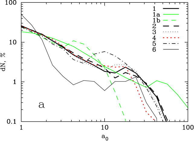
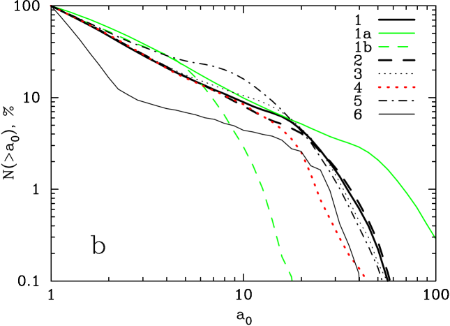
Figure 1: Probability density (a) and cumulative distribution (b) of the effective Kerr parameter ($a_{0}>1$) of the CO-cores of WR stars in binary systems with different evolutionary parameters and $k_{I}$ listed in Table 1. Numbers on the vertical axis are normalized to the total number of the cores with $a_{0}>1$, which is different for each population.

Fig. 1 presents the resulting distributions of the CO-cores of WR-stars against the value of the effective Kerr parameter.

The last column in Table 1 presents the resulting ratio of the number of the cores with the effective Kerr parameter greater than unity to the total number of the cores. Though the absolute rate of GRBs is not the subject of our study, and it cannot be inferred here, we note that the relative frequencies of GRB production in different binary evolution scenarios are reflected by the numbers in the last column of Table 1. An influence of the possible magnetic coupling between the core and the slower rotating envelope, which might brake core rotation up to several times after the end of helium burning (see, e.g., van den Heuvel & Yoon, 2007), is illustrated by population ‘1b’. For ‘1b’, we decrease the coefficient of inertia $k_{I}$; effectively, this describes some loss of the angular momentum of the core and leads to lower number of fast-rotating cores. Note that our numerical estimates agree with those of Belczynski et al. (2007) who study the evolution of Population III binaries.

For the sets of parameters, used in populations ‘1’, ‘4’, and ‘5’, Bogomazov et al. (2007) performed population synthesis and estimated absolute rates of collapse events with orbital periods less than $\sim 1$ day. This corresponds to high values of the effective Kerr parameter according with

$$a_{0}\sim 0.3\,\frac{M_{\mathrm{c}}}{M_{\odot}}\,\frac{1\,\mbox{day}}{P_{\mathrm{orb}}}\,\frac{k_{I}}{0.4}\,,$$

which follows from equations (1) and (2). Close binaries containing a black hole, a main-sequence star, or a nondegenerate star filling its Roche lobe contribute to this result with different rates. The rates obtained by them agree with the observed total GRB rate derived implying a solid angle correction for GRB emission (Podsiadlowski et al., 2004).

3 Calculation of spinar models

3.1 A two-stage collapse of a spinar

Here we describe the principles of the spinar paradigm (for more details, see Lipunov & Gorbovskoy, 2007, 2008). Consider the collapse of a rotating object. When there is no sufficient internal pressure to balance the gravitational force, the body will contract until it encounters a centrifugal barrier at a radius $R_{\mathrm{sp}}$ estimated from the relation:

$$\omega^{2}\,R_{\mathrm{sp}}=\frac{G\,M}{R_{\mathrm{sp}}^{2}}\,,$$ (3)

where $\omega$ is the angular velocity. At this point we say that a spinar forms. Actual dynamical behavior of the configuration can be very complex at this transition; however, the spinar model results in the correct amount of the energy released in the process – half of the gravitational energy. From equation (1) one gets:

$$R_{\mathrm{sp}}={a_{0}^{2}}\,\frac{G\,M}{c^{2}}\,.$$ (4)

This radius is to be considered as a characteristic size in the equatorial plane. The effective Kerr parameter is virtually constant during the first stage.

The evolution of a spinar proceeds as its angular momentum decreases because of magnetic and viscous forces producing a braking torque. A spinar can be characterized by an average magnetic field which is represented by the magnetic dipole moment $\mu$. The braking torque on a spinar can be expressed by a general formula:

$$\frac{\mathrm{d}\,{(MR^{2}\omega)}}{\mathrm{d}\,{t}}=-k_{\mathrm{t}}\,\frac{\mu^{2}}{R^{3}}\,$$ (5)

(see also Lipunov, 1992, chapter 5), where $R$ is the spinar radius and $k_{\mathrm{t}}$ is a dimensionless parameter of order of unity. Such an approach describes a maximally effective mechanism for spin-down. Note that the spinar’s rotation speeds up with decreasing spin.

The magnetic dipole moment $\mu$ can be expressed using parameter $\alpha_{\mathrm{m}}=B_{0}^{2}\,R_{0}^{4}/(6\,G\,M_{0}^{2})$ – the ratio of the magnetic energy to the gravitational energy – a measure of magnetization introduced by Lipunov & Gorbovskoy (2007). The initial value of magnetic dipole moment $\mu_{0}=B_{0}\,R_{0}^{3}/2$ can be rewritten as $\sqrt{\alpha_{\mathrm{m}}\,\,G}\,M_{0}\,R_{0}$, incorporating constants of order of unity into $\alpha_{\mathrm{m}}$. Here zero-subscripts indicate initial values of the parameters, and $B$ is the dipolar strength of the magnetic field, which approximates the actual field configuration. In the approximation of magnetic flux conservation, the magnetic parameter $\alpha_{\mathrm{m}}$ remains constant.

As the spinar contracts and its rotation speeds up, the energy-release rate increases, but as the spinar’s size approaches the size of a limiting Kerr black hole, the magnetic field squeezes up against the surface, and the spinar’s power fades away. Thus the second peak is produced. To account for the vanishing magnetic field, we use the following approximate expression (Ginzburg & Ozernoi, 1965; Lipunova, 1997; Lipunov & Gorbovskoy, 2008):

$$\mu=\mu_{0}\left(\frac{R_{0}}{R}\right)^{2}\frac{\xi(R_{0}/r_{\mathrm{g}},a_{0})}{\xi(R/r_{\mathrm{g}},a)}\,,\\ \xi(x,a)=\frac{x_{\mathrm{min}}(a)}{x}+\frac{x_{\mathrm{min}}^{2}(a)}{2\,x^{2}}+\ln\left(1-\frac{x_{\mathrm{min}}(a)}{x}\right),$$ (6)

where $r_{\mathrm{g}}=G\,M/c^{2}$ and $\xi(x,a)\approx-(x_{\mathrm{min}}/x)^{3}/3$ if $x\gg x_{\mathrm{min}}$ and $\xi(x,a)\rightarrow-\infty$ if $x\rightarrow x_{\mathrm{min}}$, with $x_{\mathrm{min}}(a)=1+\sqrt{1-a}$ for $a<1$ and $x_{\mathrm{min}}(a)=1$ for $a\geq 1$.

Lipunov & Gorbovskoy (2008) obtain the characteristic time-scale for the second stage, or the time scale of the angular momentum losses (c.f. 3 and 5):

$$t_{\mathrm{am}}=\frac{G\,M}{c^{3}}\,\frac{a_{0}^{3}}{2\,k_{\mathrm{t}}\,\alpha_{\mathrm{m}}}\,.$$ (7)

The complete set of equations (see Lipunov & Gorbovskoy, 2008) includes all the main relativistic effects near the gravitational radius: dynamics in the Kerr metric, magnetic field extinction, time dilation, and gravitational redshift. The ‘spinar engine’ posesses properties commonly considered necessary to launch jets: rotation, magnetic field, relativistic velocities and energies. These jets can be observed as GRBs. The magneto-dynamical model of the spinar provides a main-scale pattern of time evolution for a GRB, ignoring its short-scale variability. We do not make any assumptions about the specific nature of the jets, but we will imply for self-consistency that there is an efficiency of processing the burst energy to the jet, which can be about 1 per cent (see also Sect. 5.2).

3.2 Characteristics of spinar ‘light curves’

The input parameters to the model of collapse are the effective dimensionless Kerr parameter of the core, the magnetic parameter, and its mass. For example, Fig. 2 shows the distribution of the effective Kerr parameters and masses of the cores of WR stars in close binary systems for population ‘1’ (throughout the paper we denote a result from population synthesis, i.e. a set of massive cores, as a population with a corresponding number from the first column of Table 1). Only cores with $a_{0}>1$ are counted in Fig. 2. We note that for populations ‘1’-‘5’ the distribution of WR core masses with unrestricted $a_{0}$ has one peak around $7-8$ M_⊙. More massive cores have an advantage in acquiring large $a_{0}$ as they have a greater radius while synchronized (see equation (2)); this results in the multi-peak form of the mass distribution in Fig. 2. At the same time, the mass distribution itself is not very important for the results of the present work (it only shows itself in Fig. 5a as a three-branch disposition of points). For each pair $a_{0}$ and $m=M/M_{\odot}$, we set a value of $\alpha_{m}$ randomly and uniformly distributed on a logarithmic scale with limits $10^{-7}..10^{-2}$.

Figure 2: The distribution of the pre-collapse effective Kerr parameters (solid line) and the distribution of the masses (dashed line) for the collapsing WR cores with $a_{0}>1$ for population ‘1’ (see Table 1). $N_{\mathrm{total}}=8000$.

To calculate spinar temporal evolution, we solve a system of differential equations (Lipunov & Gorbovskoy, 2008) using a fourth-order Rosenbrock method (Press et al., 2002, Chap. 16) with tolerance $10^{-5}$. We start integration of equations at radius $2\times 10^{3}\,G\,M/c^{2}$. This value has little impact on the result, because the main energy output of the first peak happens at the moment of spinar formation, and the spinar radius does not depend on the initial radius (see equation 4). Simultaneously, while sampling the Scenario Machine results, we set an upper limit on the effective Kerr parameter, $a_{0}\approx 44$, to ensure that a core is not below the centrifugal barrier at the beginning of a calculation. The lower limit on $a_{0}$ is 1. Coefficient $k_{\mathrm{t}}$ in the expression for the braking torque (5) is set to $1/3$.

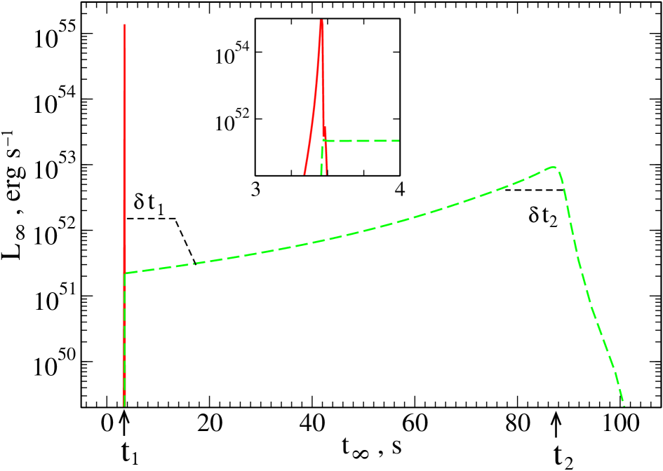
Figure 3: Energy release rate of a collapsing spinar (the sum of the solid and the long-dashed line). Initial parameters are $m=7$, $a_{0}=5$, and $\alpha_{\mathrm{m}}=10^{-4}$. Time and luminosity are in the frame of an infinite observer. Left short-dashed profile represents characteristic observed duration of the first peak. Right short-dashed horizontal line is drawn at the 0.5 level from the peak value of $L_{\infty}$. The overlaying graph zooms in a time interval near the first peak.

Each trio of parameters, $a_{0}$, $\alpha_{\mathrm{m}}$, and $m$, yields a power curve with two pulses of different strength and duration. Various patterns can be recognized, like plateaus, tails, one-peak patterns, etc.

Consider as an example the burst evolution in Fig. 3 that shows the rate of energy release as detected by an infinite observer, corrected for the gravitational redshift and time dilation. The solid line shows the dissipation rate of the kinetic energy at ‘impact’ (i.e., the halt at the centrifugal barrier); the long-dashed line shows the power released when the angular momentum is carried away. One can see that the two stages are clearly separated by the relative contribution of the two means of energy supply.

The burst pattern provides two useful temporal characteristics: the separation between peaks $t_{2}-t_{1}$ and the duration of the second peak $\delta t_{2}$. Generally, the computed duration of the first peak is very short, because it corresponds to the time-scale of a dynamic model. Thus, it should not be compared directly with a GRB jet duration. The process of a jet development or propagation is not considered or specified here. Duration of the second peak, estimated as shown in Fig. 3, might also underestimate the jet duration for the same reason.

We assume that a model represents a GRB with precursor if it satisfies the following condition: $(E_{1}/\delta t_{1})/L_{2}<1$. Here $E_{1}$ is the energy released during the first pulse, $L_{2}=L_{\infty}^{\mathrm{max}}$ – the peak value for the second pulse. $E_{1}$ is obtained by integrating over the time interval during which $L_{\infty}$ is greater than $l\times L_{\infty}^{\mathrm{max}}$, where $l$ is a fractional value. We usually set $l$ to 0.5 or 0.1.

A constraint on the actual duration of the first peak $\delta t_{1}$ comes from observational data. It is widely accepted that the short and the long GRBs have different underlying mechanisms or progenitors (Norris et al., 2001; Balázs et al., 2003; Fox et al., 2005). Swift data indicate that long and short GRBs have different redshift distributions with different median values of $z$: $0.4$ for short GRBs and $2.4$ for long GRBs (O’Shaughnessy et al., 2008; Bagoly et al., 2006). We assume that both the first and the second peaks of the calculated models contribute to the class of long GRBs. Burlon et al. (2008) study data for Swift GRBs with precursor with measured redshifts, all of them having rest-frame precursor durations between 3 and 20 seconds. Thus, we attribute factitious durations to the first peaks, generating real values distributed randomly and uniformly in the above limits.

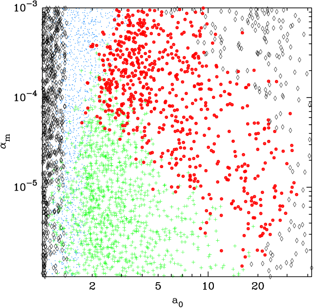
Figure 4: Magnetic parameter versus initial effective Kerr parameter for different classes of GRBs: with precursor (big red dots), with the stronger first peak (green pluses), with single peak (black diamonds), and merged peaks (small blue dots). Color is seen in the electronic version. For a comparison, the reader is referred to the diagram in figure 2 of  Lipunov & Gorbovskoy (2008).

4 Results

For each population from Table 1, we calculate 8000 models within wide limits of $\alpha_{\mathrm{m}}$ ($10^{-7}..10^{-2}$). Among the calculated models we can distinguish four classes of GRBs. These are two classes with separate peaks: GRBs with precursor and GRBs with a stronger first peak; third, GRBs with one pulse, produced by models with $a_{0}$ either very large or close to unity; the last, GRBs with very close pulses, meaning that the time separation between the pulses is less than the maximum of two values: $0.1$ s (an arbitrary chosen small value) and $(\delta t_{1}+\delta t_{2})/2$. Fig. 4 shows distributions of the initial model parameters for different classes of GRBs. Here precursors satisfy the following condition: $1>(E_{1}/\delta t_{1})/L_{2}>0.01$. If a precursor is very weak, then a GRB is re-classified and becomes a single-peak GRB (diamonds in the top right corner of Fig. 4).

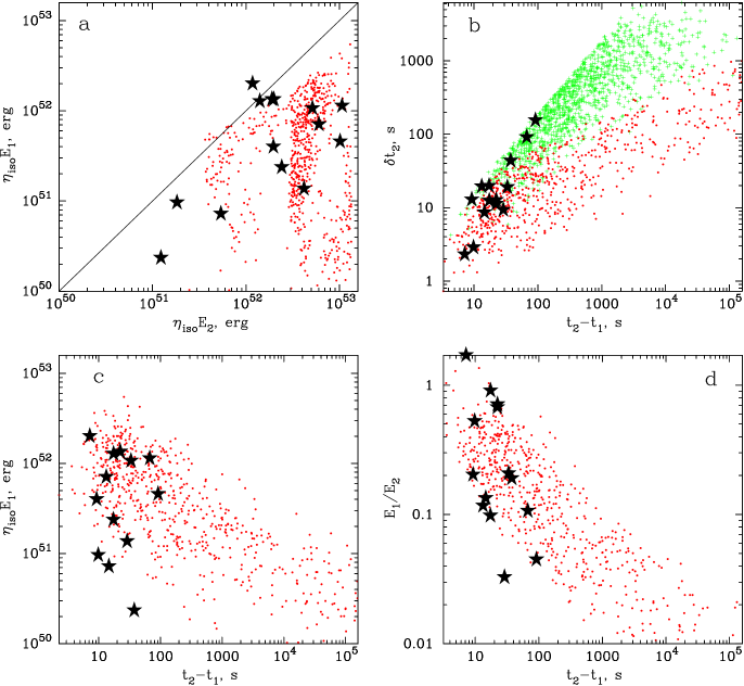
Figure 5: (a) Energy of the first peak vs. energy of the second peak; (b) duration of the second peak vs. separation between the peaks; (c) energy of precursor vs. separation; (d) precursor-to-main-peak energy ratio vs. separation. Population ‘1’ from Table 1 is used. Dimensionless coefficient $\eta_{\mathrm{iso}}=0.01$ for both peaks. Magnetic parameter $10^{-6}<\alpha_{\mathrm{m}}<10^{-3}$. Pluses (green in the electronic version) in (b) represent results for the models with a stronger first peak. Stars are plotted for the data taken from Burlon et al. (2008): rest-frame magnitudes $E_{\mathrm{iso}}$, mostly in $15-150$ keV, separation times, calculated as ($T_{1,\mathrm{main}}-T_{1,\mathrm{prec}})/(1+z)$, and durations of the main peaks ($T_{2,\mathrm{main}}-T_{1,\mathrm{main}})/(1+z)$.

In Fig. 5 we present characteristic time and energy distributions for a class of models identified as GRBs with precursor. The initial parameters for the models in Fig. 5 are taken from population ‘1’ (see Sect. 2). The energies and durations of the peaks are calculated for a level of $0.5$ of the peak luminosity (for illustration see Fig. 3). In Fig. 5 the energy of pulses is given as $\eta_{\mathrm{iso}}\,E_{\mathrm{P}}\equiv E_{\mathrm{iso}}$, where $E_{\mathrm{P}}$ is the calculated energy of a peak, P $=1$ or $2$, and $E_{\mathrm{iso}}$ is the rest-frame isotropic bolometric energy, which can be derived from values observed in a spectral energy band. Here we set $\eta_{\mathrm{iso}}=0.01$ for both peaks in order to cover with the modeled points the area that is occupied by the observed values adopted from Burlon et al. (2008) (stars in Fig. 5). Coefficient $\eta_{\mathrm{iso}}$ incorporates our freedom in choosing level $l$ as well as the actual efficiency of the gravitational collapse, and the fact that there are two jets.

Burlon et al. (2008) study a sample of GRBs with precursor activity detected by Swift and with known redshifts. All GRBs with precursors belong to a class of long GRBs, as also found for the BATSE catalogue by Koshut et al. (1995). We use the data from Table 1 of Burlon et al. (2008) except for GRB 070306 that has two precursors (see Sect. 5.1). The observed time intervals are recalculated to the rest-frame using known redshifts. One can see that the separation times $t_{2}-t_{1}$ between the peaks calculated in the spinar model reproduce very well the observed time lags and that longer lags are also produced. From the practical point of view it is worth noting that separation times calculated numerically agree with values $t_{\mathrm{am}}$ defined by (7) quite closely, within an accuracy of 10% for most of the models. Formula (7) can be rewritten as

$$t_{am}\approx 20\,\frac{M}{10\,M_{\odot}}\,\left(\frac{a_{0}}{3}\right)^{3}\,\left(\frac{\alpha_{\mathrm{m}}}{10^{-4}}\right)^{-1}\,\left(\frac{k_{\mathrm{t}}}{1/3}\right)^{-1}\,\mathrm{s}.$$ (8)

In Fig. 5b, we also show by pluses results for the models with a stronger first peak. Some of these models can manifest themselves as events with a precursor due to some dispersion of $\eta_{\mathrm{iso}}$ and differences in the efficiencies of the two peaks. The scatter of the observed values (stars in Fig. 5) can be also caused by different efficiencies in the sources. In the context of Fig. 5b, we notice that a correlation with slope about $1$ between emission duration time and previous quiescent time in the observer frame was found by Ramirez-Ruiz & Merloni (2001) (see their figure 3b) who investigated long and bright BATSE bursts containing at least one quiescent interval in their time history (they did not sample precursor events). Their slope roughly coincides with the overal slope of the star-distribution in Fig. 5b.

Table 2: Relative frequency of GRBs with precursor for different ranges of the modeled separation time between the precursor and the main peak.

Population	$t_{2}-t_{1}$, s
	$<100$	$100-10^{3}$	$100-10^{6}$
1	0.08	0.04	0.10
1a	0.11	0.07	0.12
1b	0.08	0.09	0.14
2	0.09	0.05	0.10
3	0.08	0.05	0.12
4	0.09	0.05	0.11
5	0.07	0.05	0.17
6	0.02	$<$0.01	0.03

In Table 2 we give the approximate ratios of the number of GRBs with precursor to the number of all GRBs for different binary evolution parameters. The fraction of the models with precursor of separation $<100$ s is $8-10$ per cent for most of the populations. All GRBs include two-peak GRBs, single peak GRBs, and GRBs with very close peaks. To calculate these ratios, only precursors that are ‘strong enough to be detected’ are counted; that is, they satisfy an arbitrary chosen condition: $(E_{1}/\delta t_{1})/L_{2}>0.01$.

The numbers in the Table 2 should be regarded as rough estimates, as they are based on an assumption that a modeled power curve (as, for example, in Fig. 3) provides a realistic relation between $L_{1}$ and $L_{2}$. If we halve the efficiency $\eta_{\mathrm{iso}}$ of the precursor, the relative number of precursors becomes greater but not significantly ($\sim 10$ per cent for population ‘1’, for example). To provide some glimpse of the significance of the numbers, we can say that, if we change the level for calculating peak duration and energy to $l=0.1$ and keep other parameters unchanged, then the number of GRBs with precursor drop to 6 per cent for population ‘1’.

Normalized histograms for distributions of modeled separation times and main (i.e., second) peak durations are plotted in Figs. 6 and 7. Observational data from Burlon et al. (2008) is also presented. The modeled duration of the second peak might be a minimum estimate of the actual duration because no radiation and magneto-hydrodynamic effects are incorporated in the present model of a GRB.

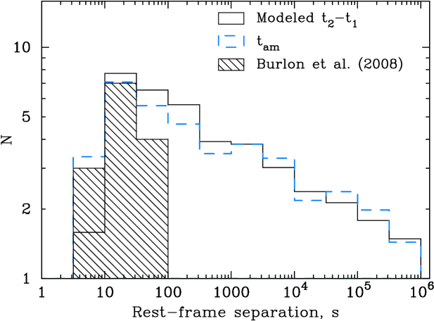
Figure 6: Distribution of the separation times between the precursor and the main pulse. Empty histograms show model estimates and are vertically scaled with the same area under the solid and the dashed line. Hatched histogram represents rest-frame separation times ($T_{1,\mathrm{main}}-T_{1,\mathrm{prec}})/(1+z)$ from Burlon et al. (2008). The set of models is the same as in Fig. 5.

Figure 7: Distribution of the duration of the main pulse. Empty histogram shows model results for events with precursors and is vertically scaled. Hatched histogram represents rest-frame duration times $(T_{2,\mathrm{main}}-T_{1,\mathrm{main}})/(1+z)$ taken from Burlon et al. (2008). The set of models is the same as in Fig. 5.

The longest observed separation between the peaks of a precursor and a main pulse, $\sim 400$ s, was reported by Koshut et al. (1995) but no conclusion about the rest-frame time separation can be made without knowing $z$. Nevertheless, our results are in apparent agreement with the data from figure 13 of Koshut et al. (1995) that shows the ratio of the precursor total counts to the main episode total counts versus separation time between detectable emission. The distribution in Fig. 8 is constructed for population ‘1’ for analogous values where we try to emulate cosmologically dilated separation times by multiplying all values $(t_{2}-t_{1})$ by a constant factor.

Figure 8: Ratio of the energy released during the precursor and the main peak versus separation time multiplied by the constant factor. Dots represent model results for GRBs with precursor for population ’1’. The average value of the redshift for long GRBs $\overline{z_{\mathrm{long}}}=2.4$. Stars are adopted from figure 13 of Koshut et al. (1995) that shows the ratio of the precursor total counts to the main episode total counts versus separation time between detectable emission for BATSE GRBs with precursor.

Summarizing, the spinar paradigm explains observed precursor separation times and predicts that there are very early precursors with rest-frame time separations more than 100 s, which is the maximum determined rest-frame separation so far (Burlon et al., 2008). Our results show that the rate of GRBs with precursor, which have separations longer by up to one order of magnitude than those observed so far, is about half the detected rate (compare the second and third columns of Table 2). The number of modeled GRBs with precursor with lead times in the range from $100$ s to $10^{6}$ s is comparable to the frequency of precursor events observed so far. At the same time, the expected average energy output of a precursor drops with increasing separation time as illustrated by Fig. 5c.

One should keep in mind that a rest-frame time interval as, for example, $100$ s, is dilated to $(1+z)\times 100$ s in the observer’s frame. At this point, an important general conclusion can be made: GRBs at high redshifts will show precursor events which should arrive $(1+z)\times 100\sim 1000$ s in advance of the main event. This prediction is very strong as it does not depend on a GRB model.

5 Discussion

The relative frequencies of the GRBs with precursor, obtained in the spinar paradigm, agree reasonably well with observational facts. Koshut et al. (1995) find precursors in $\sim 3$ per cent of BATSE long and short GRBs detected before May 1994; Lazzati (2005) finds that precursors are present in $\sim 20$ per cent of bright, long GRBs in the final BATSE catalog; Burlon et al. (2008) obtains that about $14$ per cent from 105 GRBs with measured redshift, observed by Swift before March 2008, have precursor activity. Note that these researches use different criteria for precursor search and selection. All these data agree quite well with the modeled ratios within an accuracy of $5-10$ per cent (see Table 2). Note that there is no significant difference in the ratios between the different binary evolution scenarios (for wind model W1) and different $k_{I}$. Apparently, the strong wind scenario experiences the most difficulty in describing the reported ratios (population ‘6’).

To speak of a more robust result, the spinar model provides a clear explanation of the diversity of observed time separtions between precursor and main peak, which, moreover, can be related to the main physical parameters of a collapsing object in a simple way (equation 7 or 8). To our knowledge, explaining both relatively short ($\sim 10$ s) and long ($\sim 100$ s) switch-off times presented difficulties for most of the GRB engine models (see Wang & Mészáros, 2007; Drago & Pagliara, 2007, and references therein).

Accretion has so far been neglected by us, but could be easily incorporated in the equations, as pointed out by Lipunov & Gorbovskoy (2008); this is a topic for a forthcoming paper. As a preliminary result, we found that accretion of up to $\gtrsim 1~{}$M_⊙ during the overall GRB time ($10-100$ s) does not change qualitatively any of the results presented.

5.1 Multi-precursors

Among 15 GRBs with precursor studied by Burlon et al. (2008) there is one (GRB 070306) with two precursors. The first precursor is $\sim 105$ s from the second precursor, which is ahead of the main pulse by $\sim 95$ s. Each pulse is stronger than the previous one. This GRB is not shown in the figures in the present paper.

One way to explain such a phenomenon is an unstable regime of jet with a constantly operating central engine. A mechanism of a modulated relativistic wind, resulting in long time gaps in emission, was considered by Ramirez-Ruiz et al. (2001).

Other possibilities appear if we consider the basic elements of the spinar paradigm. As we argue in the Introduction, the course of a collapse is affected by the initial distribution of the angular momentum in the rotating object. In this regard, spinar and collapsar models are ‘opposite’ options. In reality there is most probably an assortment of mixed scenarios. One possibility, provided by a particular angular momentum distribution in a pre-collapse core, is that a black hole forms first (primary pulse), then a spinar (heavy accretion disc) forms around it (second pulse), followed by a fatal collapse (hyper-accretion) of a spinar into a black hole (third pulse). Another explanation for a three-stage collapse can be that an accretion disc aggregates at some stage of a spinar evolution. Here we should mention the ‘initial jet and fallback collapsar’ scenario (Wang & Mészáros, 2007) with its characteristic disc time of $\sim 100$ s. In its context, we can speculate why the majority of GRBs with precursor (or GRBs with one or more quiescent periods, see Ramirez-Ruiz & Merloni (2001)) are not three-step events. The fallback scenario works for explosions that are not too weak or too strong according to Fryer (1999). An explosion which is too weak leads to a direct collapse to a BH, or a spinar if it rotates fast enough. Rotating progenitors possibly favor ‘direct collapse to a spinar’ without a huge explosion; this view is supported by general and computational (Monchmeyer, 1991; Yamada & Sato, 1994) arguments that rotation weakens the bounce and hence the explosion.

Numerical studies yield further options for gravitational collapse: fragmentation of a rotating collapsing body, a multiple black hole system formation (see, for example, Berezinskii et al., 1988; Imshennik, 1992; Zink et al., 2007), and its eventual merger. Such scenarios (see also King et al., 2005) can provide a burst with several pulses, but are beyond the scope of the present work.

5.2 Lower limit on a precursor energy

Let us provide some relations for the energetics of the precursor jet. The precursor jet is apparently the first to break through a shell that probably surrounds the central object. Lipunov & Gorbovskoy (2008) arrive at a condition for a jet to penetrate the surrounding shell. The jet breaks through if the momentum imparted on a part of the shell is greater than the momentum corresponding to the escape velocity:

$$\beta\,E_{\mathrm{P}}=E_{\mathrm{jet}}^{\mathrm{p}}>\frac{\Omega_{\mathrm{s}}}{4\pi}\,M_{\mathrm{shell}}\,\sqrt{\frac{2GM_{\mathrm{core}}}{R_{\mathrm{shell}}}}\,c\,,$$ (9)

where $\beta$ is the efficiency of processing the energy of the collapse to the pushing jet, $c$ is the speed of the jet, which is approximately the speed of light, ${\Omega_{\mathrm{s}}}/{4\pi}$ is the portion of the shell’s surface subject to the jet. Substituting universal constants, one has:

$$E_{\mathrm{jet}}^{\mathrm{p}}\gtrsim 6\times 10^{50}\,\frac{{\Omega_{\mathrm{s}}}}{0.01\times 4\pi}\,m_{\mathrm{shell}}\,\left(\frac{R_{\mathrm{shell}}}{2\times 10^{3}\,r_{\mathrm{g}}}\right)^{-1/2}\,\mathrm{erg},$$ (10)

where $m_{\mathrm{shell}}$ is in solar masses.

Now consider the relations for the observed jet:

$$E_{\mathrm{jet}}^{\mathrm{ob}}=k_{\gamma}\,E_{\mathrm{jet}}^{\mathrm{p}},\quad E_{\mathrm{jet}}^{\mathrm{ob}}\equiv E_{\mathrm{iso}}\,\frac{\Omega_{\mathrm{ob}}}{4\pi}\,.$$ (11)

It is natural to assume that the energy of the jet punching the shell is not the same as that of the observed $\gamma$-jet and to introduce a factor $k_{\gamma}<1$ between them, which depends, among other things, on the spectral band observed. Here $\Omega_{\mathrm{ob}}$ is the solid angle corresponding to the observed jet’s opening angle, $E_{\mathrm{iso}}$ is the rest-frame isotropic bolometric energy, which can be derived from the values observed in a spectral energy band.

From the above we derive the minimum value $E_{\mathrm{iso}}$ that corresponds to a jet still capable of going through the shell:

$$E_{\mathrm{iso}}(min)=6\times 10^{52}k_{\gamma}\,\frac{\Omega_{\mathrm{s}}}{\Omega_{\mathrm{ob}}}\,m_{\mathrm{shell}}\,\left(\frac{R_{\mathrm{shell}}}{2\times 10^{3}\,r_{\mathrm{g}}}\right)^{-1/2}\,\mathrm{erg}.$$ (12)

Let us now illustrate this with some numbers. Fig. 5a possibly indicates that $E_{\mathrm{iso}}(min)\sim 10^{50}$ erg from the data of Burlon et al. (2008). Comparing with equation (12), one can obtain an implicit estimate of $k_{\gamma}$ for the observational data mentioned as low as $0.1-1$ per cent, if $\Omega_{\mathrm{s}}\sim\Omega_{\mathrm{ob}}$ and $m_{\mathrm{shell}}\sim 1$.

In Sect. 4, we introduced the parameter $\eta_{\mathrm{iso}}$ to match the modeled energy of the pulses with the rest-frame isotropical values $E_{\mathrm{iso}}$. We estimated it as $\eta_{\mathrm{iso}}\sim 0.01$. Using (9) and (11), $\eta_{\mathrm{iso}}$ can be expressed as follows:

$$\eta_{\mathrm{iso}}\equiv\frac{E_{\mathrm{iso}}}{E_{\mathrm{P}}}=\frac{4\pi}{\Omega_{\mathrm{ob}}}\,k_{\gamma}\,\beta\,.$$ (13)

If the half-opening angle of a jet $\sim 0.1$ rad (e.g., Meszaros, 2006) and $k_{\gamma}\sim 0.001-0.01$ then $\Omega_{\mathrm{ob}}~{}\sim 0.03~{}\mathrm{sr}\sim 4\,\pi/400$ and we come at an estimate for the effieciency of processing the energy of the collapse to the jet in the shell: $\beta\sim\eta_{\mathrm{iso}}\sim 0.01$.

6 Conclusion

Currently, much effort is put into numerical computations of GRBs and simulations of jets emerging from rotating magnetized configurations, to name just a few, by Lyutikov (2006); Barkov & Komissarov (2008); McKinney & Blandford (2009); Takiwaki et al. (2009) and others. We believe that the progress with the spinar mechanism for GRBs demands a further development by means of a MHD simulation.

In the present work, we calculate many models of two-stage spinar evolution provided that fast rotating stellar cores are produced in binary systems due to a tidal synchronization mechanism. The pre-collapse parameters of WR stars are calculated by the Scenario Machine dedicated to the population synthesis of binary systems (Lipunov et al., 1996a; Lipunov et al., 2007).

We analyse the resulting set of GRBs, which can be classified into different classes. For GRBs with precursor, separation times between the precursor and the main pulse are fully consistent with observational data. We find that precursor events with the rest-frame time separation from the main pulse $<100$ s occur in about $10$ per cent of the modeled GRB events, for the weak wind scenarios of binary evolution and independently of the poorly established value of $k_{I}$. This rate, however, depends on the specifics of the jet generation and its reliability is limited by the framework of our simple model. Taking this into account, we think the modeled rate agrees very well with the observed values. Comparison of the time and energetic characteristics of the modeled bursts with the observational data for GRBs with measured redshifts (Burlon et al., 2008) is made and a good general agreement is found.

We predict that very early precursors with a rest-frame time separation more than 100 s should exist, and the number of GRBs with precursor with separations in the range from $100$ s to $1000$ s is about half the number of those observed so far. Super-early primary pulses, up to $10^{6}$ s, are also found in the model; they, however, may be too weak to be detected or to develop as a jet.

Finally, whether or not the present model works in all cases, the observational evidence is that rest-frame separation times of $\sim 100$ s take place. High-redshift long GRBs, up to $z\gtrsim 10$, are expected to be detected by future experiments (e.g., Salvaterra et al., 2008). Thus, we confidently expect precursor events arriving up to $\gtrsim$1000 seconds in advance of the main GRB episode.

References

- Bagoly et al. (2006) Bagoly Z., Mészáros A., Balázs L. G., Horváth I., Klose S., Larsson S., Mészáros P., Ryde F., Tusnády G., 2006, A&A, 453, 797
- Balázs et al. (2003) Balázs L. G., Bagoly Z., Horváth I., Mészáros A., Mészáros P., 2003, A&A, 401, 129
- Barkov & Komissarov (2008) Barkov M. V., Komissarov S. S., 2008, MNRAS, 385, L28
- Belczynski et al. (2007) Belczynski K., Bulik T., Heger A., Fryer C., 2007, ApJ, 664, 986
- Berezinskii et al. (1988) Berezinskii V. S., Castagnoli C., Dokuchaev V. I., Galeotti P., 1988, Nuovo Cimento C Geophysics Space Physics C, 11, 287
- Bisnovatyi-Kogan (1971) Bisnovatyi-Kogan G. S., 1971, Soviet Astronomy, 14, 652
- Bisnovatyi-Kogan & Blinnikov (1972) Bisnovatyi-Kogan G. S., Blinnikov S. I., 1972, Ap&SS, 19, 119
- Bogomazov et al. (2007) Bogomazov A. I., Lipunov V. M., Tutukov A. V., 2007, Astronomy Reports, 51, 308
- Bogomazov et al. (2008) Bogomazov A. I., Lipunov V. M., Tutukov A. V., 2008, Astronomy Reports, 52, 463
- Brown et al. (2000) Brown G. E., Lee C.-H., Wijers R. A. M. J., Lee H. K., Israelian G., Bethe H. A., 2000, New Astronomy, 5, 191
- Burlon et al. (2008) Burlon D., Ghirlanda G., Ghisellini G., Lazzati D., Nava L., Nardini M., Celotti A., 2008, ApJ, 685, L19
- Drago & Pagliara (2007) Drago A., Pagliara G., 2007, ApJ, 665, 1227
- Fox et al. (2005) Fox D. B., Frail D. A., Price P. A., Kulkarni S. R., Berger E. E., 2005, Nature, 437, 845
- Fryer (1999) Fryer C. L., 1999, ApJ, 522, 413
- Ginzburg & Ozernoi (1965) Ginzburg V. L., Ozernoi L. M., 1965, Soviet Journal of Experimental and Theoretical Physics, 20, 689
- Ginzburg & Ozernoi (1977) Ginzburg V. L., Ozernoi L. M., 1977, Ap&SS, 50, 23
- Gunn & Ostriker (1969) Gunn J. E., Ostriker J. P., 1969, Physical Review Letters, 22, 728
- Hirschi et al. (2005) Hirschi R., Meynet G., Maeder A., 2005, A&A, 443, 581
- Hoyle & Fowler (1963) Hoyle F., Fowler W. A., 1963, MNRAS, 125, 169
- Imshennik (1992) Imshennik V. S., 1992, Soviet Astronomy Letters, 18, 194
- Izzard et al. (2004) Izzard R. G., Ramirez-Ruiz E., Tout C. A., 2004, MNRAS, 348, 1215
- King et al. (2005) King A., O’Brien P. T., Goad M. R., Osborne J., Olsson E., Page K., 2005, ApJ, 630, L113
- Koshut et al. (1995) Koshut T. M., Kouveliotou C., Paciesas W. S., van Paradijs J., Pendleton G. N., Briggs M. S., Fishman G. J., Meegan C. A., 1995, ApJ, 452, 145
- Lazzati (2005) Lazzati D., 2005, MNRAS, 357, 722
- LeBlanc & Wilson (1970) LeBlanc J. M., Wilson J. R., 1970, ApJ, 161, 541